Modelling the Quality of Bathing Waters in the Adriatic Sea

Abstract

The aim of this study is to develop a relocatable modelling system able to describe the microbial contamination that affects the quality of coastal bathing waters. Pollution events are mainly triggered by urban sewer outflows during massive rainy events, with relevant negative consequences on the marine environment and tourism and related activities of coastal towns. A finite element hydrodynamic model was applied to five study areas in the Adriatic Sea, which differ for urban, oceanographic and morphological conditions. With the help of transport-diffusion and microbial decay modules, the distribution of Escherichia coli was investigated during significant events. The numerical investigation was supported by detailed in situ observational datasets. The model results were evaluated against water level, sea temperature, salinity and E. coli concentrations acquired in situ, demonstrating the capacity of the modelling suite in simulating the circulation in the coastal areas of the Adriatic Sea, as well as several main transport and diffusion dynamics, such as riverine and polluted waters dispersion. Moreover, the results of the simulations were used to perform a comparative analysis among the different study sites, demonstrating that dilution and mixing, mostly induced by the tidal action, had a stronger effect on bacteria reduction with respect to microbial decay. Stratification and estuarine dynamics also play an important role in governing microbial concentration. The modelling suite can be used as a beach management tool for improving protection of public health, as required by the EU Bathing Water Directive.

1. Introduction

Microbiological contamination of marine water bodies is one of the biggest environmental concerns in coastal zones subjected to rapid population growth [1]. Faecal bacteria (e.g., Escherichia coli and Enterococci) originating from human faeces and organic waste in the sewage, as well as animal faeces in run-off, disposed of in the water bodies without any sanitation systems, constitute essential sources for the marine environmental contamination [2,3]. Consequently, human health can be seriously endangered and a bad bathing water quality can have adverse effects on the tourist industry and many recreational and economic activities [4]. Storm runoff has become one of the major sources of pollutant loading, including pathogens, pesticides, heavy metals and nutrients to the coastal recreational waters [5,6]. In the last decades, extraordinary strong storm events have become more and more regular in many areas with the prediction of further rise in their frequency [3]. During these uncontrolled storm events, combined sewer overflows (CSOs) discharge high concentrations and loads of E. coli and intestinal enterococci bacteria in the receiving water bodies, where faecal bacteria concentrations can easily exceed the bathing water quality standards [7].

At the European level the Bathing Water Directive (BWD, [8]) and the corresponding transposition law within each EU nation, define threshold levels for intestinal enterococci and Escherichia coli concentrations to prevent the health risks associated with bathing in marine and freshwaters. The BWD establishes the guidelines for bathing water monitoring and classification, the management, and the provision of information to the public. In an efficient water quality preservation program, mitigating the microbiological contamination of marine waters requires an integrated assessment, whenever necessary, to enable decision-makers to adopt adequate mitigation actions and to explore the consequences of various management options for protecting public health [1,9].

Various best practices and innovative solutions have been developed to control and improve the outflow of microbial contamination from urban centres near the beaches coming from the result of mixing domestic wastewater and drained storm water: (i) sedimentation tanks; (ii) discharge point far from the shoreline; (iii) biosensor to monitor in real time; (iv) forecast models of pollutant dispersion in the sea.

The sedimentation tank, adequately sized, is used to collect mixing domestic wastewater and drained storm water in order to return them to suitable purification systems and then discharge them in a cleaner way into the sea. This kind of intervention might not be adapted in all water systems [10]. Submarine outfalls are commonly used to enhance the dispersion of treated sewage, thus avoiding pollution from the shoreline. The transferral of the final discharge point far from the shoreline improves pollution dispersion, preserving the impacts on the bathing waters in all meteorological conditions [11,12].

Recently, efforts have been done to adopt chemical sensors for achieving higher sensitivity to, and selectivity of, pollutants in water. These devices, equipped with multisensors for detecting pollutants, chemicals and E. coli concentration into the waters, can be used for an online water analysis of water quality [13], and the Bayesian method has been used to identify optimal sensor distribution to solve a contamination detection and location problem [14]. Among sensors, biosensors have been developed for food safety and environmental applications (e.g., specific detection of pathogens such as E. coli) because of their advantageous rapidity and ease of use. The polymeric matrices interact with specific amino-acids on bacteria surface antigens, and through these interactions, it is possible to imprint specific regions of bacteria as fingerprints for their detection [15,16].

Limiting the exposure to polluted water also requires a quantitative understanding of storm runoff impact on coastal water quality and predictive models that can forecast the water quality for timely management decisions [17]. In this regard, oceanographic models constitute a useful tool for determining the concentration of faecal bacteria in nearshore bathing waters [18,19,20] and to calculate the risk for human health caused by microbial pollution [21,22]. Simulation of water circulation and the transport processes affecting coastal areas requires the use of numerical models at high spatial resolution capable of representing complex morphological and bathymetric features, as well as several anthropogenic constructions (piers, artificial reefs, breakwaters, jetties) present along the coast. Moreover, the correct representation of the coastal dynamics requires high temporal resolution to describe processes occurring at a short time scale, like tidal fluctuation and flash river floods (e.g., [23]). The simulation of nearshore water quality during and after sewer overflows requires high-resolution models as well as detailed information concerning water discharge and microbial concentration input values [7]. The last requirement is crucial in many coastal sites, where the sewer outflows are not continuously monitored or where illegal sewer connectors discharge into the sea. Therefore, all coastal simulations must be supported by an adequate dataset for their implementation and validation.

By understanding the dynamics associated with faecal contamination, it is possible for managers and policymakers to incorporate those findings to develop sound sampling strategies and attenuation measures in order to avoid bathing area closures for prolonged and unnecessary periods of time. Normally, the application of numerical dispersion models is used to support the traditional monitoring methods based on field observations and laboratory analysis in order to link information concerning the hydrodynamic circulation, environmental parameters and the microbiological features of an area [7,11].

Most of the previous modelling studies have been limited to one coastal system and they lack an integrated, comprehensive evaluation in different environments. In this study, we describe a relocatable modelling system for assessing microbial pollution in coastal areas which consists of a hydrodynamic model, a transport and diffusion module and a microbial decay module. The adopted approach realises a seamless transition between different spatial scales, from the river mouth to the open sea, and adopts a high spatial and temporal resolution of the forcing and boundary conditions that drive the simulations. The model is evaluated against observations in the coastal areas, illustrating the capability of this tool in simulating the water circulation, as well as the dispersion and decay of microbial pollutants. The model has been applied to five different coastal areas located on both the western and the eastern sides of the Adriatic Sea, a region of the Mediterranean Sea considered very sensitive area due to the heavy organic, eutrophication substances and other pollutants discharged through the main rivers [11,24,25,26]. Alongside these forms of pollution, the problem of microbial contamination is also particularly relevant for the Adriatic Sea coast, where several urban settlements, popular bathing locations and tourist centres are located [26,27,28,29,30].

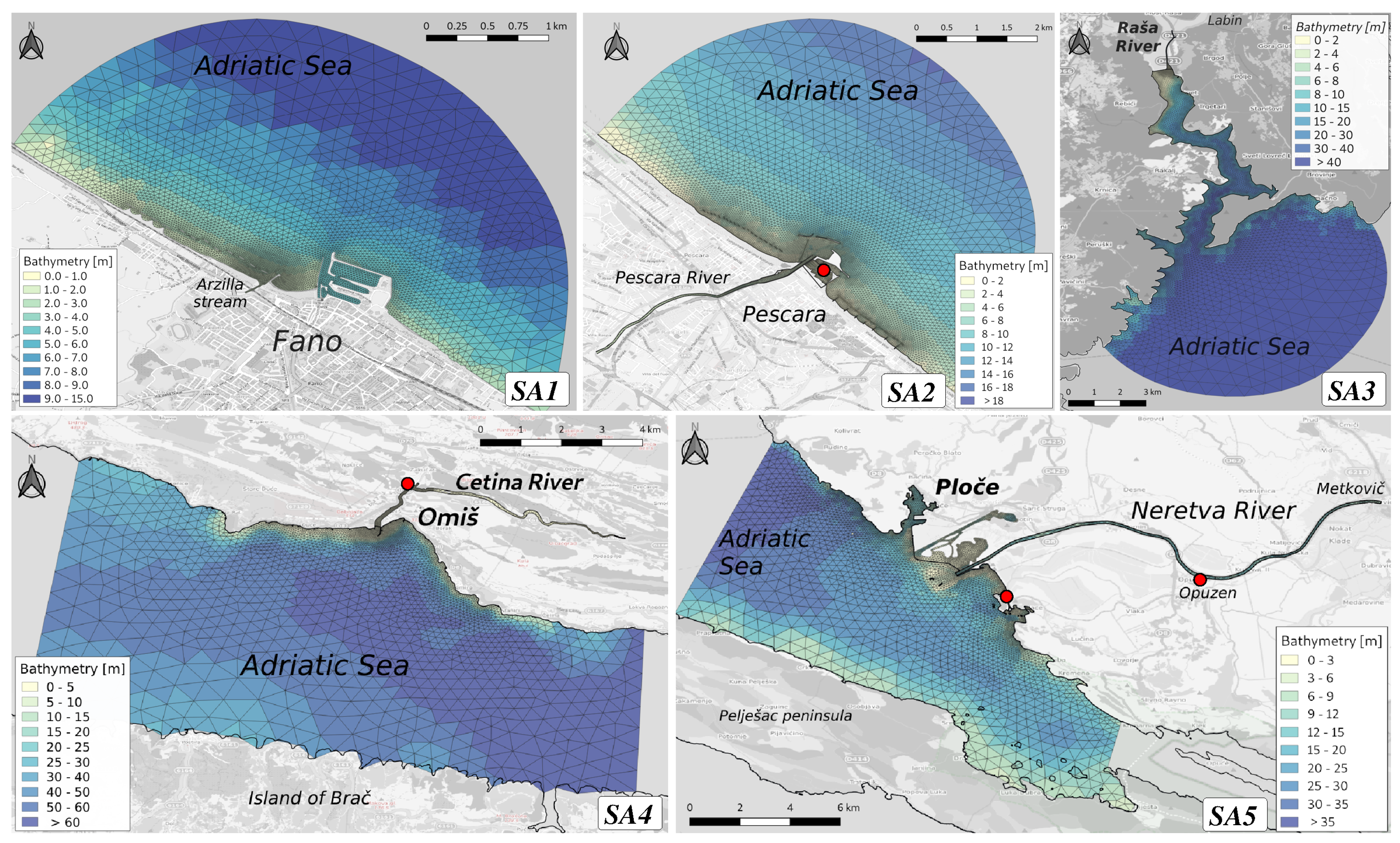
Study Areas

This study focuses on five target coastal areas located in the Adriatic Sea, an 800-km-long, 150-km-wide elongated semi-enclosed basin interacting with the Mediterranean Sea through the Otranto Strait in the southern part (Figure 1). The main forcings of the Adriatic basin circulation are the wind (influenced by the complex local orography and small scale processes), the strong buoyancy resulting from the freshwater inputs injected by the rivers and the tidal waves propagating from the Mediterranean Sea. The general surface circulation of the Adriatic Sea may be described as a large-scale cyclonic meander, with a northerly flow along the eastern coast and a southerly return flow along the western coast and a double gyre configuration in the central and southern parts of the basin [31,32].

As in other countries, increasing population and rapid urban development along the coastline of the Adriatic Sea have caused a dramatic increase in sewage discharge into rivers and the sea [26,28]. Most of this sewage has undergone no more than primary treatment and threatens the health of aquatic ecosystems and directly and indirectly affects human health and recreational opportunities along the coast [10,24,34]. Bathing waters and recreational activities are a resource of great economic and environmental importance and their safety is a primary goal in the management of the coastal area. Even if Italy has adopted criteria that is highly restrictive in terms of quality of bathing waters and monitoring, recent studies underlined the persistence of many critical situations in various parts of the Adriatic coasts [11,25,29], and consequently, bathing has been prohibited at different points.

A wide variety of coastal environments are present along the coastline of the Adriatic Sea. The eastern and western sides of the Adriatic Sea greatly differ in appearance: the western coast is largely sedimentary, with mild sloping and sandy beaches, while the eastern coast is composed of many islands and headlands and is generally rugged and rocky. All areas investigated in this study are coastal zones located near urban settlements and influenced by the discharge of a river collecting wastewaters from the local sewage system. As indicated in Figure 1, they are:

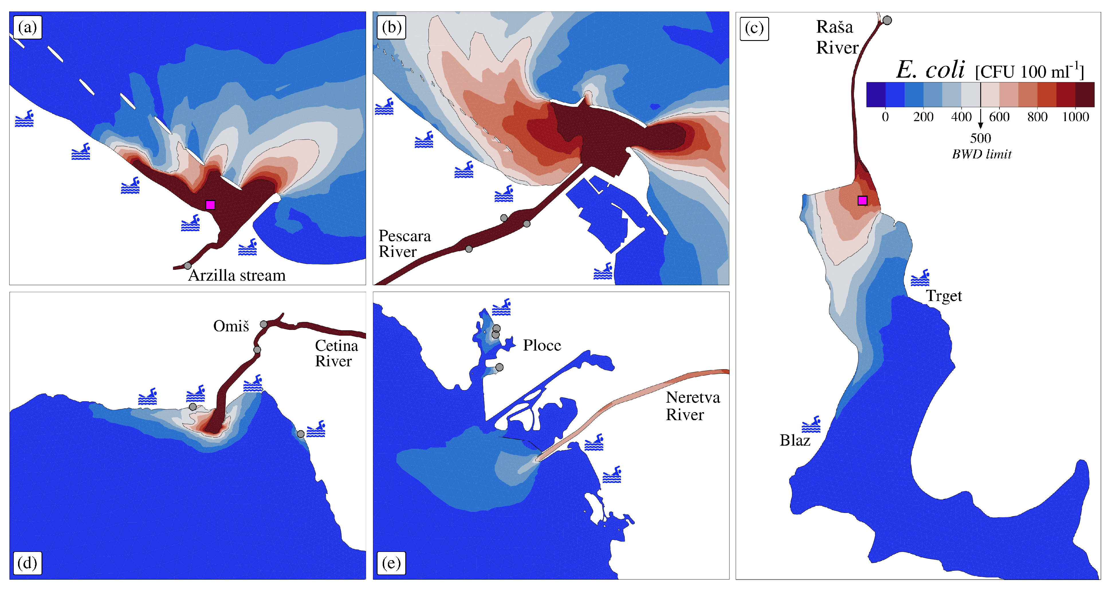
• SA1: the coast of Fano at the mouth of the Arzilla stream (Marche region, Italy);
• SA2: the coast of Pescara at the mouth of the Pescara River (Abruzzo region, Italy);
• SA3: the fjord-like system of the Raša River (Istria region, Croatia);
• SA4: the coast of Omiš at the Cetina River mouth (Split–Dalmatia region, Croatia);
• SA5: the Ploče coast with the Neretva Estuary (Dubrovnik–Neretva region, Croatia).

These environments give a representative picture of the different coastal systems situated around the Adriatic basin covering a wide range of urban, hydrological and oceanographic conditions. An overview of the study sites is provided in Figure 2 and a comprehensive description of their characteristics is reported in Section 2.2.

2. Materials and Methods

2.1. Model Description

The modelling framework presented here is based on the System of HydrodYnamic Finite Element Modules (SHYFEM, [35]) code, an open-source unstructured ocean model for simulating hydrodynamics and transport processes at very high resolution. The modelling suite consists of:

• a 3D hydrodynamic model, that describes currents and mixing of water mass in the system;
• a transport and diffusion module, that simulates the dispersion of solute and microorganisms through the system;
• a microbial decay module, which defines the decay of microorganisms considering various environmental conditions.

The horizontal discretization of the state variables is carried out with the finite element method, with the subdivision of the numerical domain in triangles varying in form and size. Such a method has the advantage of representing, in detail, complicated bathymetry and irregular boundaries in coastal areas. Thus, it can solve the combined large-scale oceanic and small-scale coastal dynamics in the same discrete domain by using unstructured meshes. In the following sections, the single modules are described in detail.

2.1.1. The Hydrodynamic Model

The 3D hydrodynamic finite element model is based on the solution of primitive equations and previously applied on several transitional environments, coastal and shallow basins. The model has already been applied to simulate hydrodynamics in the Mediterranean Sea [36], in the Adriatic Sea [37] and in several coastal systems ([38], and references therein). Ref. [39] demonstrated the good performance of the SHYFEM model in simulating water levels, currents, salinity, and water temperature in the Adriatic Sea.

The hydrodynamic model is the “engine” that transports and mixes all ecosystem constituents, including the water itself. The model solves, in a 3D formulation, the shallow water equations, which for an arbitrary vertical layer l, are the following:

$$\begin{array}{c}\frac{\partial U_l}{\partial t}+u_l\frac{\partial U_l}{\partial x}+v_l\frac{\partial U_l}{\partial y}-f{V}_l=-g{h}_l\frac{\partial \zeta }{\partial x}-\frac{g{h}_l}{{\rho }_0}\frac{\partial }{\partial x}{\int }_{-H_l}^{\zeta }{\rho }^{\prime }dz-\frac{h_l}{{\rho }_0}\frac{\partial p_a}{\partial x}\\ \hspace{1em}\hspace{1em}\hspace{1em}\hspace{1em}\hspace{1em}\hspace{1em}+\frac{1}{{\rho }_0}\left({\tau }_x^{top\left(l\right)}-{\tau }_x^{bottom\left(l\right)}\right)+\frac{\partial }{\partial x}\left(A_H\frac{\partial U_l}{\partial x}\right)+\frac{\partial }{\partial y}\left(A_H\frac{\partial U_l}{\partial y}\right)+\frac{\partial }{\partial z}\left(A_v\frac{\partial U_l}{\partial z}\right)\end{array}$$

(1)

$$\begin{array}{c}\frac{\partial V_l}{\partial t}+u_l\frac{\partial V_l}{\partial x}+v_l\frac{\partial V_l}{\partial y}+f{U}_l=-g{h}_l\frac{\partial \zeta }{\partial y}-\frac{g{h}_l}{{\rho }_0}\frac{\partial }{\partial y}{\int }_{-H_l}^{\zeta }{\rho }^{\prime }dz-\frac{h_l}{{\rho }_0}\frac{\partial p_a}{\partial y}\\ \hspace{1em}\hspace{1em}\hspace{1em}\hspace{1em}\hspace{1em}\hspace{1em}+\frac{1}{{\rho }_0}\left({\tau }_y^{top\left(l\right)}-{\tau }_y^{bottom\left(l\right)}\right)+\frac{\partial }{\partial x}\left(A_H\frac{\partial V_l}{\partial x}\right)+\frac{\partial }{\partial y}\left(A_H\frac{\partial V_l}{\partial y}\right)+\frac{\partial }{\partial z}\left(A_v\frac{\partial V_l}{\partial z}\right)\end{array}$$

(2)

$$\frac{\partial \zeta }{\partial t}+\sum _l\frac{\partial U_l}{\partial x}+\sum _l\frac{\partial V_l}{\partial y}=0$$

(3)

with $U_l,V_l$ the horizontal transport at each layer (integrated velocities), f the Coriolis parameter, $p_a$ the atmospheric pressure, g the gravitational acceleration, $\zeta$ the sea level, ${\rho }_0$ the average density of sea water, $\rho ={\rho }_0+{\rho }^{\prime }$ the water density, $\tau$ the internal stress term at the top and bottom of each layer, $h_l$ the layer thickness, $H_l$ the depth at the bottom of layer l. The Smagorinsky’s formulation [40,41] is used to parameterize the horizontal eddy viscosity ($A_H$). For the computation of the vertical viscosities ($A_v$), a turbulence closure scheme was used. This scheme is an adaptation of the k-$ϵ$ module of the General Ocean Turbulence Model described in [42].

Velocities are computed in the centre of the grid element, whereas water levels are computed at element vertices (nodes). The model uses a semi-implicit algorithm for integration over time, which has the advantage of being unconditionally stable for gravity waves, bottom friction and Coriolis terms, and allows transport variables to be solved explicitly. The model adopts automatic sub-stepping over time to enforce numerical stability for advection and diffusion. A more detailed description of the model equations and the discretization method is given in [35,43].

2.1.2. The Transport and Diffusion Module

The 3D Eulerian transport-diffusion model solves the following equation:

$$\begin{array}{c}\frac{\partial C_l}{\partial t}+u_l\frac{\partial C_l}{\partial x}+v_l\frac{\partial C_l}{\partial y}+w_l\frac{\partial C_l}{\partial z}=\frac{\partial }{\partial x}\left(K_l^H\frac{\partial C_l}{\partial x}\right)+\hfill \\ \hfill \hspace{1em}\hspace{1em}\hspace{1em}\hspace{1em}\hspace{1em}\hspace{1em}\hspace{1em}\hspace{1em}\hspace{1em}\hspace{1em}\hspace{1em}\hspace{1em}\hspace{1em}\hspace{1em}\hspace{1em}\hspace{1em}\hspace{0.17em}\frac{\partial }{\partial y}\left(K_l^H\frac{\partial C_l}{\partial y}\right)+\frac{\partial }{\partial z}\left(K_l^V\frac{\partial C_l}{\partial z}\right)+E-K_d{C}_l\end{array}$$

(4)

where $C_l$ is the concentration at the layer l of the solute (tracer, salinity, water temperature); $u_l$, $v_l$ and $w_l$ are the horizontal and vertical component of the currents; $K_l^H$ and $K_l^V$ are respectively the horizontal and vertical turbulent diffusion coefficients calculated the former with the Smagorinsky formulation [40] and the latter calculated by the k-$ϵ$ turbulence closure model; E is the sink/source term; $K_d$ is the decay rate. The transport and diffusion equation is solved with a first-order explicit scheme based on the total variational diminishing scheme.

In the case of salinity, the source/loss term E represents the difference between evaporation and precipitation through the water surface. The evaporation rate is determined by the bulk aerodynamic transfer method [44] using measurements of air temperature, relative humidity, wind speed, air pressure and simulated water temperature. In the case of water temperature, E represents the heat source through the water surface $Q/\rho c_w{h}_l$, where $\rho$ is the water density, $c_w$ is the specific heat of water ($c_w$ = 3991 J kg${}^{-1}$ ${}^{°}\mathrm{C}$${}^{-1}$) and $h_l$ is the depth of fluid layer. Q is the heat flux between the atmosphere and the sea computed by the energy-radiation balance considering short and longwave radiation, heat flux generated by the evaporation-condensation process and heat flux generated by the convection and conduction process.

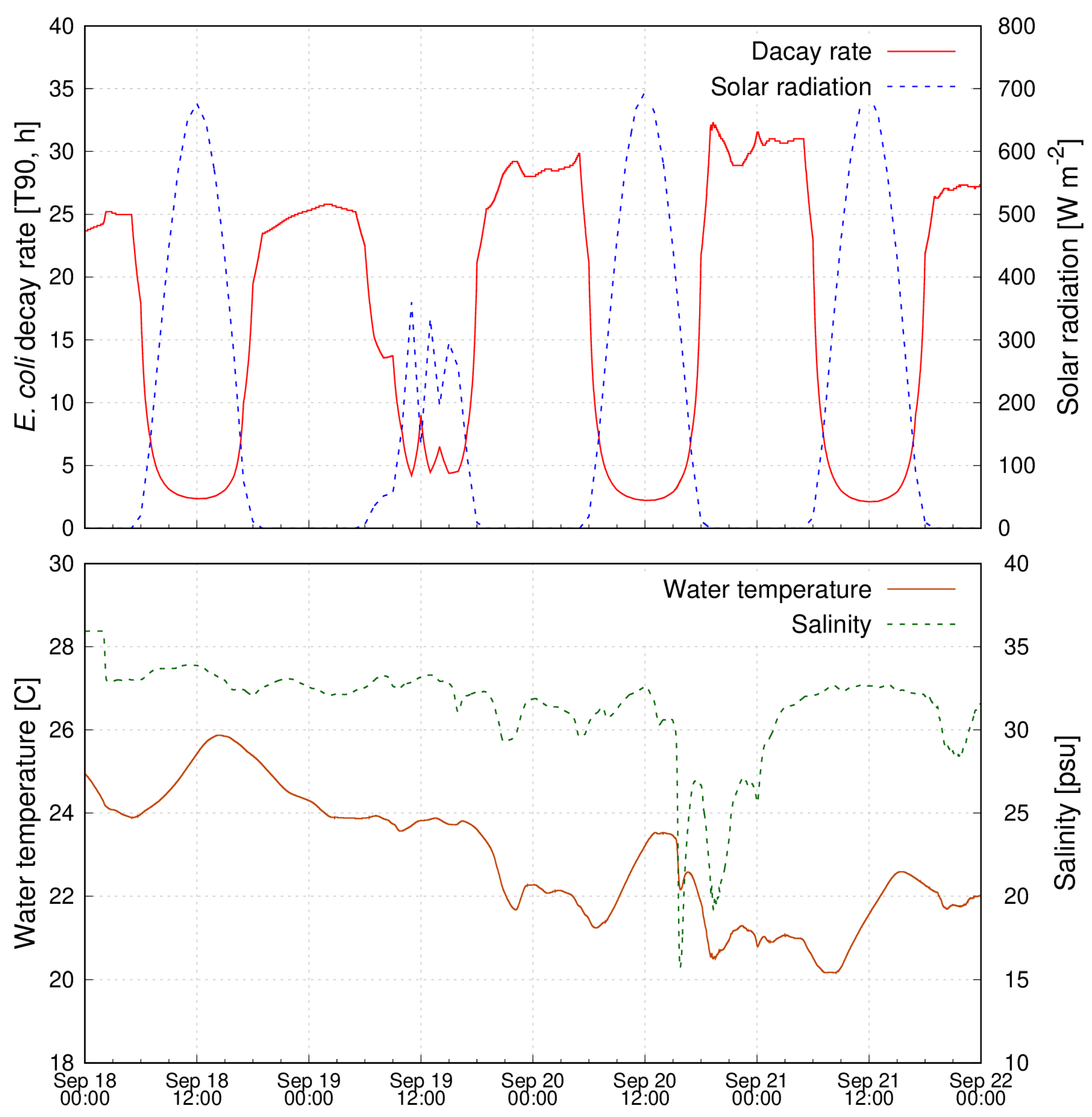
2.1.3. The Microbial Decay Module

In marine coastal environments, the fate of free-living faecal bacteria in the water column is approximated as an Eulerian tracer (term C in Equation (4)) subjected to dilution and a decay relationship. Following Ostoich et al. [12], in this study, the decay rate ($K_d$) is considered variable in space and time as a function of the environmental conditions, e.g., water temperature, salinity, water turbidity and UV radiation. To implement this equation, we followed that proposed by Chapra [45], where the total loss rate for bacteria can be read as:

$$K_d=K_{base}+K_{solar}$$

(5)

where $K_{base}$ is the base mortality rate and $K_{solar}$ is the loss rate due to solar radiation. Other significant processes, like settling and adsorption in suspended particulate matter, are not considered in this study. The $K_{base}$ term [46] for sea waters can be presented as:

$$K_{base}=(0.8+0.02S_l)1.{07}^{(T_l-20)}$$

(6)

where $S_l$ and $T_l$ are the salinity and water temperature at layer l, respectively.

The term $K_{solar}$ is proportional to the surface light energy ($I_0$) through a constant $\alpha$, approximately equal to 1 [47]. Using the Lambert–Beer law to model the exponential decay of light in a well-mixed layer, $K_{solar}$ can be calculated as:

$$K_{solar}=\frac{I_0}{k_{e}H}(1-e^{-k_{e}H})$$

(7)

where $k_e$ is the light extinction coefficient in the water and H is the water depth. According to Feitosa et al. [48], the approach of Mancini [46] is recommended for estimating bacterial decay rates under day and nighttime conditions and considering the combined influences of temperature and salinity. The simulated bacterial concentration is highly sensitive to the prescribed decay rate ([20], and reference therein), but in highly dynamic environments, dilution generally has a higher effect on bacterial reduction than decay [21,49]. The bacteria decay module was tested using ambient values of solar radiation, water temperature and salinity registered in Fano in Summer 2019. The obtained decay rate (T90, defined as the time at which 90% of the bacterial population is no longer detectable) is presented in Figure 3. The decay rate varies from 3 h during the night to a peak daily value of more than 30 h with clear sky conditions. The decay rate increases with the salinity and with the water temperature. Such T90 values were within the proposed ranges of Feitosa et al. [48] and Ostoich et al. [12].

The decay equations have been integrated into the model for each node and in the middle of each layer, considering a value of 1 for the extinction coefficient, increasing progressively the total depth of the column from surface to bottom. At each time step, the model simulates the dispersion of faecal bacteria from the sewer outflow into the coastal waters.

2.2. Model Implementation

The model runs in a full 3-D baroclinic mode with the water column discretized in zeta or hybrid (mixed sigma and zeta) layers with varying thickness (see the site-specific settings illustrated below). We performed several numerical experiments for simulating hydrodynamic conditions and dispersion of E. coli in the five study sites. The discharge of the sewage outlet is simulated with an Eulerian approach, where the concentration of E. coli is prescribed in outflow and the impact of the concentration is evaluated on the coast. The simulations were forced:

• at the sea open boundary by sea temperature, salinity, water level and currents conditions obtained from the TIRESIAS operational system of the Adriatic Sea [39]. Such an unstructured oceanographic model reproduces in detail the general circulation in the Adriatic Sea, as well as several relevant coastal dynamics, like tidal amplification, saltwater intrusion, storm surge and riverine water dispersion;
• at the sea surface by meteorological data (air temperature, solar radiation, humidity, cloud cover, mean sea level pressure, wind speed and direction) from the high-resolution MOLOCH model [50]. The MOLOCH model is implemented with a horizontal grid spacing of 1.25 km, and with 60 atmospheric levels and 7 soil levels and provides the meteorological parameters at hourly frequency;
• at the river boundary by water discharge timeseries computed from observed water levels through calibrated stage-discharge relationships;
• at the pollutant sources by bacteria concentration and water volume according to the available site-specific data.

For the free surface, a water flux is used containing evaporation minus precipitation and river discharge. For computing the water temperature, the air-sea heat fluxes are parameterised by the Coupled Ocean-Atmosphere Response Experiment (COARE) 3.0 bulk algorithm [51]. Also, the drag coefficient for the momentum transfer of wind in the hydrodynamic model is computed according to the COARE 3.0 bulk formulae [51]. The bottom drag coefficient is computed using a logarithmic formulation via bottom roughness length, set homogeneous over the whole model domain to a value of 0.01 m [52]. Unless specified differently, due to a lack of available observations at the river boundary the water temperature adapts to the environmental value inside the basin river and the inflow salinity is fixed to a constant value of 0.1 psu. For the same reason, unless specified differently, a constant concentration of 100,000 CFU 100 mL${}^{-1}$ was imposed at the source points during overflow events. Such value is in line with what reported in the literature ([7], and references therein).

The numerical model simulates the water circulation field, the water temperature, and the salinity by representing the physical processes occurring in the coastal areas of the Adriatic Sea, for example, tidal propagation, wind-induced currents and set up, water, heat and salt fluxes, thermohaline stratification, and vertical mixing. The simulations were performed for selected summer periods of 2019 and 2020.

In all cases, the numerical domain considers the area of interest and a larger part of the coastal and shelf seas. To adequately resolve the river-sea continuum, the grids also include the lower part of the considered river. The bathymetry interpolated onto the numerical grids was obtained by merging high-resolution site-specific datasets covering the area of interest with the composite EMODNet dataset [33] for the outer open sea. A description of the different study areas, together with site-specific details of the model implementation, is reported below.

2.2.1. Fano Coast and Arzilla Stream

The town of Fano is located along the Italian coast in the central Adriatic Sea and it covers an area of 121 km${}^2$ with 62,000 inhabitants and high urbanization. The coast of Fano is low and sandy and characterized by several artificial protections against beach erosion. The touristic harbour of Fano is located on the right side of the river mouth. The Arzilla stream has a torrent-like character with water discharge ranging from less than 1 m${}^3$ s${}^{-1}$ up to 30 m${}^3$ s${}^{-1}$. The Arzilla stream collects sewages from inland and Fano combined sewer outflow and it discharges them into the sea, near one of the most popular beaches during the summer season. Heavy rainfall often causes the overflow of the local sewage network that collects the microbial load from Fano town. Every time that a sewer outflow occurs, the bathing activity in Fano is closed based on the potential risk of faecal microbial contamination [53].

The resolution of the unstructured grid (8675 triangular elements) ranges from a few meters at the Arzilla stream mouth, up to 1.5 km at the open sea (Figure 2). The dimension of the finite elements covering the coastal area near the beaches is about 20 m. The water column is discretized in 15 vertical layers with variable thickness ranging from 0.5 m, in the topmost 3 m, to 1 m in the deeper layers (the maximum depth is 12 m). An hourly discharge time series obtained from water level measured 10 km upstream is prescribed at that river boundary and an estimated water discharge of 50 L s${}^{-1}$ was imposed at the CSO when active (starting and ending times of sewer outflow are constantly monitored). Observed E. coli concentration was applied at the river open boundary.

2.2.2. Pescara Coast and River

Pescara, located along the coast in the central Adriatic Sea, is the largest and, with about 190,000 residents, the most populated urban settlement in the Abruzzo region. The coast is low and sandy and the beach extends to both the north and south sides of the Pescara River mouth. The coast is protected from beach erosion by emerged (in the northern part) and submerged (in the southern part) artificial reefs. The river mouth is delimited by hard structures consisting of a dike on its left side, the touristic harbour on the right side and a breakwater located at approximately 400 m from the river end. The average discharge of the Pescara River is 57 m${}^3$ s${}^{-1}$. During heavy rainfall events that exceed the capacity of the local sewage systems, the Pescara river receives, in its final stretch (3.5 km from the mouth), wastewater through 8 principal CSOs.

The numerical grid consists of 14,394 triangular elements with a resolution up to 10 m and includes the Pescara River (up to 4 km upstream of the mouth where the hydrological monitoring station is located) and a coastal area extending for about 4 km to the north and the south from the river (Figure 2). All artificial coastal structures were considered in the domain. In the present implementation, the model runs in the zeta layer configuration, with 20 vertical layers of increasing thickness, from 0.5 m in the topmost layers, up to 2 m in the deepest ones (the maximum depth is 18 m). Freshwater discharge at a 15-min frequency was available to force the model at the river boundary. Measured or estimated wastewater discharge volumes were imposed at the sewer outflows.

2.2.3. Raša River Canal

The Raša River canal is a 14 km-long and 700 m-wide canal, with a depth ranging from 1 m at the river mouth to 50 m at the sea boundary. This fjord-like environment receives freshwater mainly from the Raša River, which has an average discharge of about 5 m${}^3$ s${}^{-1}$ and peak values exceeding 100 m${}^3$ s${}^{-1}$ during flood events. Microbial pollution originates mainly from the city of Labin, which discharges partially treated wastewaters in the Krapanj canal flowing into the Raša River near its mouth, and from the Raša settlement which discharges untreated wastewaters at the mouth of the river.

The model application required a detailed bathymetric dataset interpolated on a numerical mesh with a horizontal resolution up to 10 m (Figure 2). The numerical model domain consists of 16,303 triangular elements and considers the lower part of the river, the whole fjord and part of the shelf sea. However, the high horizontal resolution is not enough to correctly describe hydrodynamics in this area. The vertical resolution and discretization become important when passing from really shallow and meandering zones, like the inner river, to the shelf and, finally, to the open sea. In this model application, we used a hybrid vertical coordinate system with 10 sigma layers in the upper 10 m and 2 m thick zeta layers in the deeper part. The choice of the hybrid system was driven by the need of resolving stratification, even in the northern shallow part of the system where the river flows, as well as ensuring an adequate vertical resolution in the deeper part. Hourly water discharge values obtained from a monitoring station of Mutvica-Most located 6 km upstream of the river boundary were imposed in the numerical experiments. Water temperature and salinity continuously measured with 30-min frequency were used as boundary conditions of the Raša River. The estimated wastewater volume discharged in Labin and Raša for 2020 amounts to 322,024 and 150,000 m${}^3$ year${}^{-1}$, respectively. Due to the lack of more detailed information, a continuous flow of wastewater was imposed at the boundaries.

2.2.4. Omiš Coast and Cetina River

Omiš is a coastal town in the Dalmatia region of Croatia, located where the Cetina River meets the Adriatic Sea. The city has a population of about 15,000 inhabitants and is surrounded by sandy beaches and small pebble coves. The average discharge of the Cetina River is 18 m${}^3$ s${}^{-1}$ with peak values reaching more than 300 m${}^3$ s${}^{-1}$. The drainage system in the Omiš agglomeration is a combined drainage system consisting of a submarine outlet (1600 m offshore at a depth of 60 m) discharging treated wastewater and 8 pumping stations (overflow elements) discharging untreated wastewaters in the Cetina River and along the coast during heavy rain events.

The numerical computation has been carried out on a spatial domain that represents part of the Cetina River (up to the discharge monitoring station of Tisne, 8 km upstream the mouth), the coastal area with the bathing sites and a portion of the sea limited southward by the island of Brač (Figure 2). The unstructured grid is made of 6406 triangular elements with a resolution ranging from 25 m close to the river mouth to 750 m in the open sea. The vertical discretization is based on a hybrid approach with 6 sigma layers in the topmost 10 m and 26 unevenly distributed zeta layers, with thicknesses ranging from 2 to 5 m in the deeper open sea (the maximum depth of the grid is 72 m). An hourly discharge time series obtained from water level measured at Tisne was prescribed at that river boundary. The estimated wastewater volume discharged at the submarine outflow is 1,300,000 m${}^3$ year${}^{-1}$ and the pumping stations have a capacity ranging from 10 to 150 L s${}^{-1}$. Due to the lack of more detailed information, a continuous flow of wastewater was imposed at the boundaries.

2.2.5. Ploče Coast and Neretva Estuary

The transnational Neretva River flows near the port-town of Ploče in Croatia and represent one of the principal sources of freshwater in the Adriatic Sea with an average water discharge of about 300 m${}^3$ s${}^{-1}$. In this study, we considered only the lower part of the river in the Croatian territory from the city of Metković downstream. The area has around 35,000 inhabitants, and a wastewater system is partially established only in cities Ploče, Metković and Opuzen, but without treatment plants. In Ploče, there are three outlets into the sea, two of which are located in the urban part of the city, and the third is located in the area of the Port of Ploče. In Opuzen and Metković, all the untreated water flows into the Neretva River, while wastewaters in Ploče are discharged into the sea.

Figure 2 reports the unstructured grid of the SHYFEM application, which considers the Neretva Estuary up to 20 km upstream the mouth (where the discharge monitoring station of Metković is located), nearby wetlands and part of the sea constrained by the coast and the Pelješac peninsula. The grid consists of 9601 elements with a horizontal resolution varying from 50 m in the river and near the coast, to 750 m in the outer sea. Like many other coastal systems worldwide, the Neretva Estuary is subjected to the upstream extension of the mixing zone, with a consequent increase of the salt content in aquifers and surface waters [54]. To adequately account for the two-layer estuarine dynamics, the water column is represented by a hybrid vertical coordinate system consisting of 10 sigma layers in the upper 10 m and 18 zeta layers with a thickness of 2 m (the maximum depth of the grid is 44 m). Hourly water discharges obtained from water levels observed in Metković were imposed at the river boundary. The estimated wastewater volume discharged in Metković, Opuzen and Ploče for 2020 amounts to 364,000, 70,000 and 210,000 m${}^3$ year${}^{-1}$, respectively. Due to the lack of more detailed information, a continuous flow of wastewater was imposed at the point sources. No information about the amount of wastewater discharged into the Neretva River in Bosnia and Herzegovina was available.

3. Results and Discussion

3.1. Evaluation of the Modelling System

The applications of the SHYFEM model to the five study areas in the Adriatic Sea were validated by comparing various parameters. The model evaluation is limited by the availability of site-specific observations.

3.1.1. The Observational Datasets

The different study areas are monitored by several observational networks, which differ for the observed parameters, type of monitoring instruments and frequency of acquisition. The monitored parameters used in the validation procedures are grouped into the following three categories:

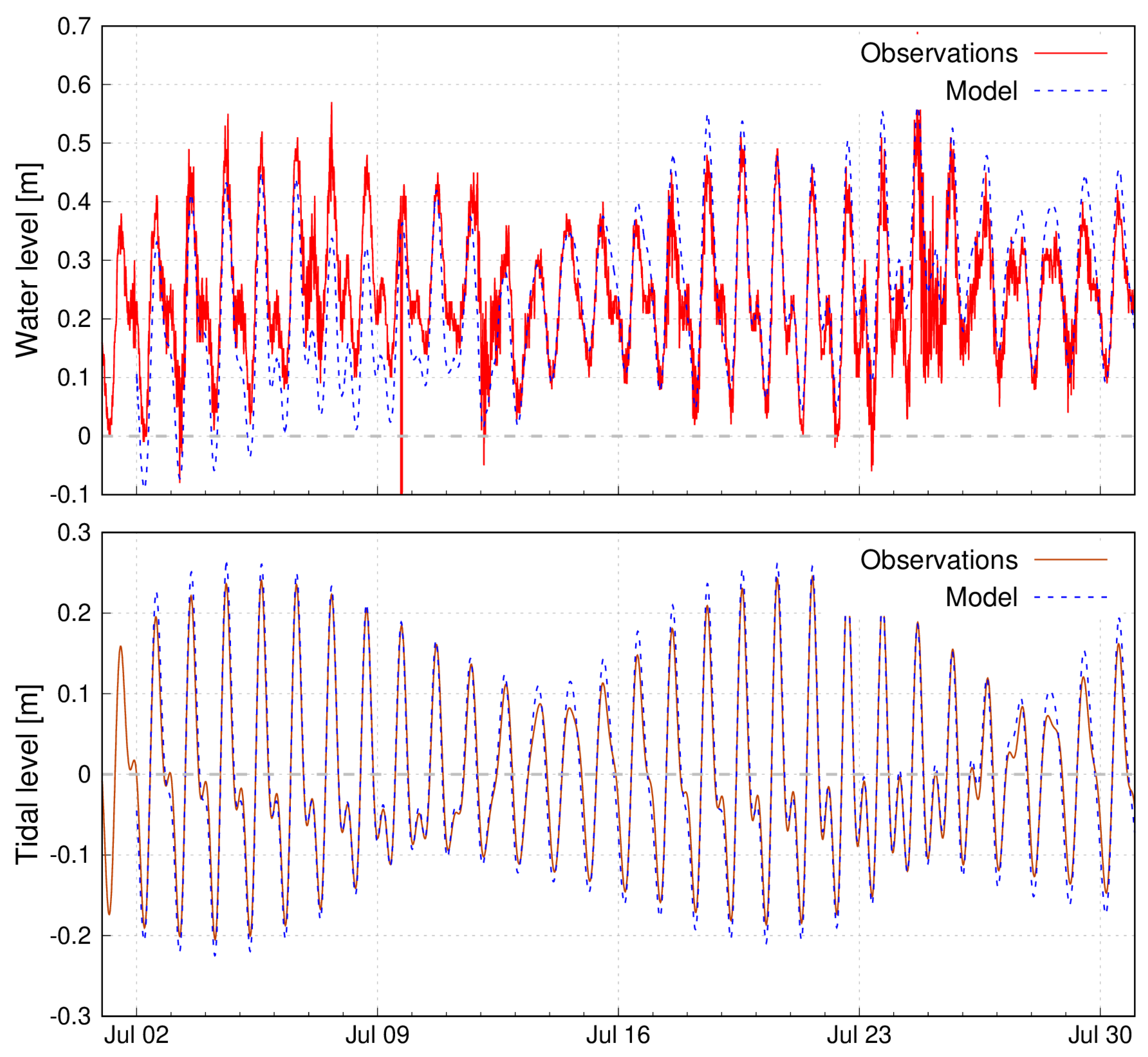
• hydrodynamic: water levels;
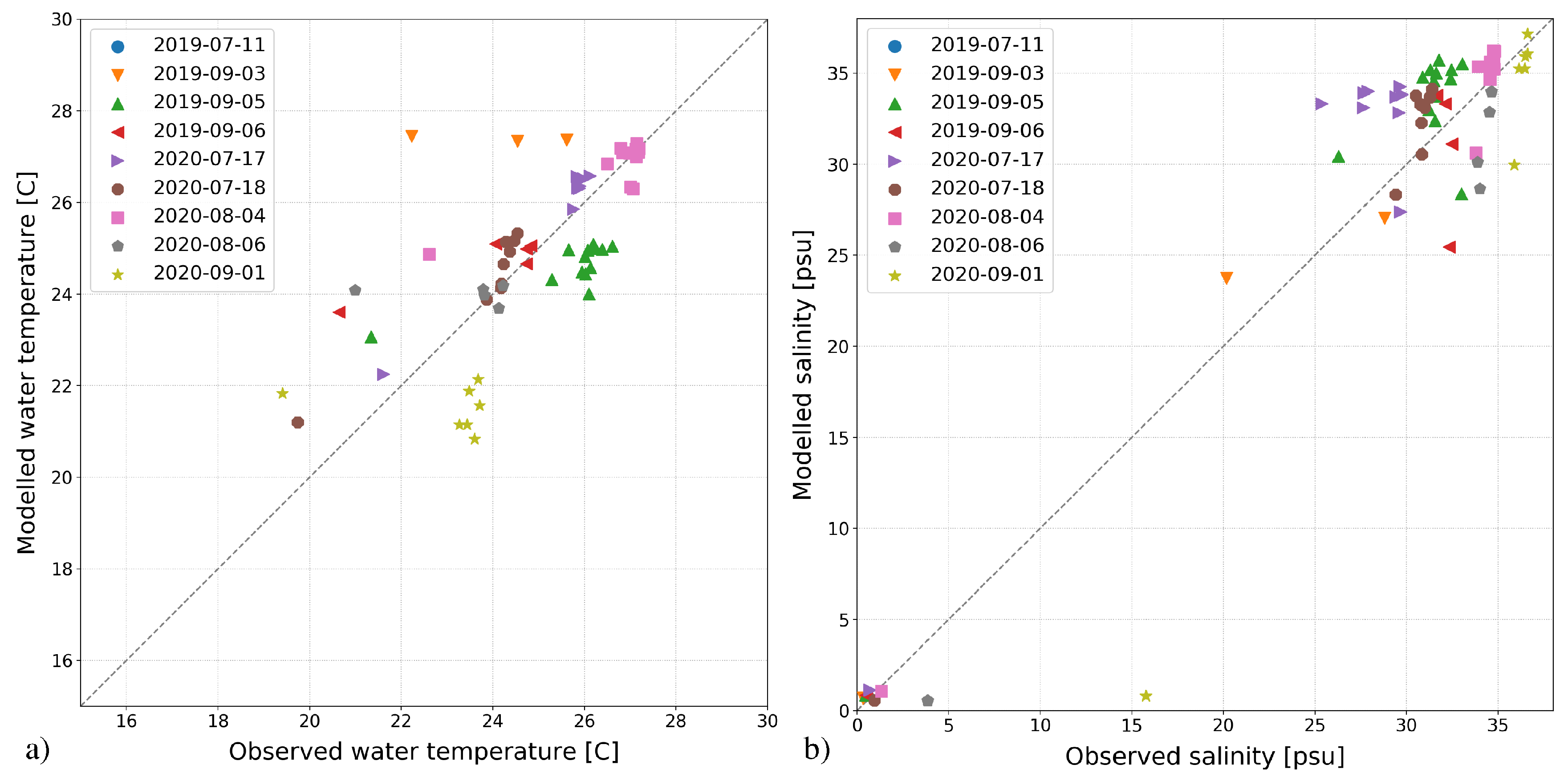
• physicochemical: water temperature and salinity;
• microbial: faecal bacteria (E. coli and intestinal enterococci) concentration.

The main characteristics of the available dataset in the five study areas are presented in

Table 1. Description of the observational datasets used for validating the modelling suite.

Study Area	Hydrodynamic	Physicochemical	Microbial
Fano coast and Arzilla stream	None	Mid-column water temperature and salinity from water samples collected at the river mouth and along three coastal transects with points at 50, 100, 150, 200 and 250 m from the coastline. Nine monitoring surveys were performed in the summer of 2019 and 2020.	Mid-column E. coli concentration from water samples collected at the river mouth and along three transects with points at 50, 100, 150, 200 and 250 m from the coastline. Nine monitoring surveys were performed in the summer of 2019 and 2020.
Pescara coast and Pescara River	Water levels measured in the Pescara harbour at a 15-min frequency (2020)	Surface water temperature values measured in the Pescara harbour at a 15-min frequency (2020)	None
Raša River canal	None	Surface water temperature and salinity from water samples collected at the river mouth and along three transects with points at 200, 400 and 600 m from the river mouth, and at two popular touristic sites located at 1.5 and 3.4 km from the river mouth. Four monitoring surveys were performed in October and November 2020.	Surface E. coli concentration from water samples collected at the river mouth and along three transects with points at 200, 400 and 600 m from the river mouth, and at two popular touristic sites located at 1.5 and 3.4 km from the river mouth. Four monitoring surveys were performed in October and November 2020.
Omiš coast and Cetina River	Hourly water levels from Omiš, 1.4 km upstream of the river mouth (2020).	None	None
Ploče coast and Neretva Estuary	Hourly water levels measured in the Neretva Estuary at Opuzen, about 12 km upstream of the river mouth, and at Ušće, along the coast at 2.4 km from the river mouth (2020).	None	None

.

The monitoring stations in Pescara, Omiš–Cetina and Ploče–Neretva study areas are indicated with red dots in Figure 2. The location of the physicochemical and microbial monitoring stations in the Fano–Arzilla and Raša River canal sites are shown in Figure 9a,b, respectively.

3.1.2. Model Assessment

The model performance was evaluated in terms of the difference between the average of simulated and observed values (BIAS), the root mean squared error (RMSE) and the Pearson product-moment correlation coefficient (R). For the concentration of E. coli, the root mean squared logarithmic (base 10) error (RMSLE) was used instead of RMSE [7]. Following the subdivision proposed for the observations, the model evaluation is presented firstly for hydrodynamics, and afterwards for the physicochemical characteristics of the coastal waters, and lastly, for the microbial pollution.

Hydrodynamic Assessment

Concerning the hydrodynamic assessment, the model results were compared with water levels recorded in Pescara, Omiš–Cetina and Ploče–Neretva study areas. The water level is here used to evaluate the hydrodynamic model performance. Observed and simulated time series were processed with a tidal harmonic analysis tool based on the least-squares fitting [55] to separate the tidal and the residual contributions to the total sea level. The statistics of the simulated values (total and tidal water levels) for the three study sites are reported in

Table 2. Statistical analysis of simulated water levels at three study areas in terms of RMSE, BIAS and R. Statistics are reported for both the total water level and tidal level.

Study Area	Station Name	RMSE (m)	BIAS (m)	R
Pescara	Pescara harbour	0.17/0.02	0.02/0	0.81/0.99
Omiš–Cetina	Omiš	0.09/0.03	0.04/0	0.72/0.96
Ploče–Neretva	Ušće	0.08/0.02	−0.07/0	0.79/0.98
	Opuzen	0.09/0.02	−0.07/0	0.77/0.98

.

The model reproduced the water levels variability observed in Pescara (top panel in Figure 4) well, even if it is not able to capture the very high-frequency fluctuations, probably generated inside the harbour by resonance phenomena. RMSE, BIAS and R for the total water level are 0.17 m, 0.02 m and 0.81, respectively. However, the model simulated the tidal fluctuation (bottom panel in Figure 4), which is the main driver of the sea-level variability in this area, with very high accuracy (RMSE = 0.02 m and R = 0.99).

The results of the model application to the Omiš–Cetina were compared with the water level continuously measured near the city of Omiš. The statistical parameters reported in Table 2 demonstrate that the model captures the sea-level variability in the investigated area, which was mostly determined by the tidal action. RMSE and R are 0.09 and 0.72 for the total water level and 0.03 and 0.96 for the tidal level.

The numerical model reproduced the water level also in the Ploče–Neretva study area (Table 2) well, with RMSEs of 0.08 and 0.02 m for the total water level and the tidal level, respectively. The results of the tidal harmonic analysis revealed that the model captures the observed tidal amplification along the river estuary, even if it is slightly overestimating the amplitude of the K1 diurnal constituent. Generally, the comparison with the tide gauge data confirmed the good performance of the SHYFEM model in simulating sea levels and tidal propagation in the Adriatic Sea [39,52].

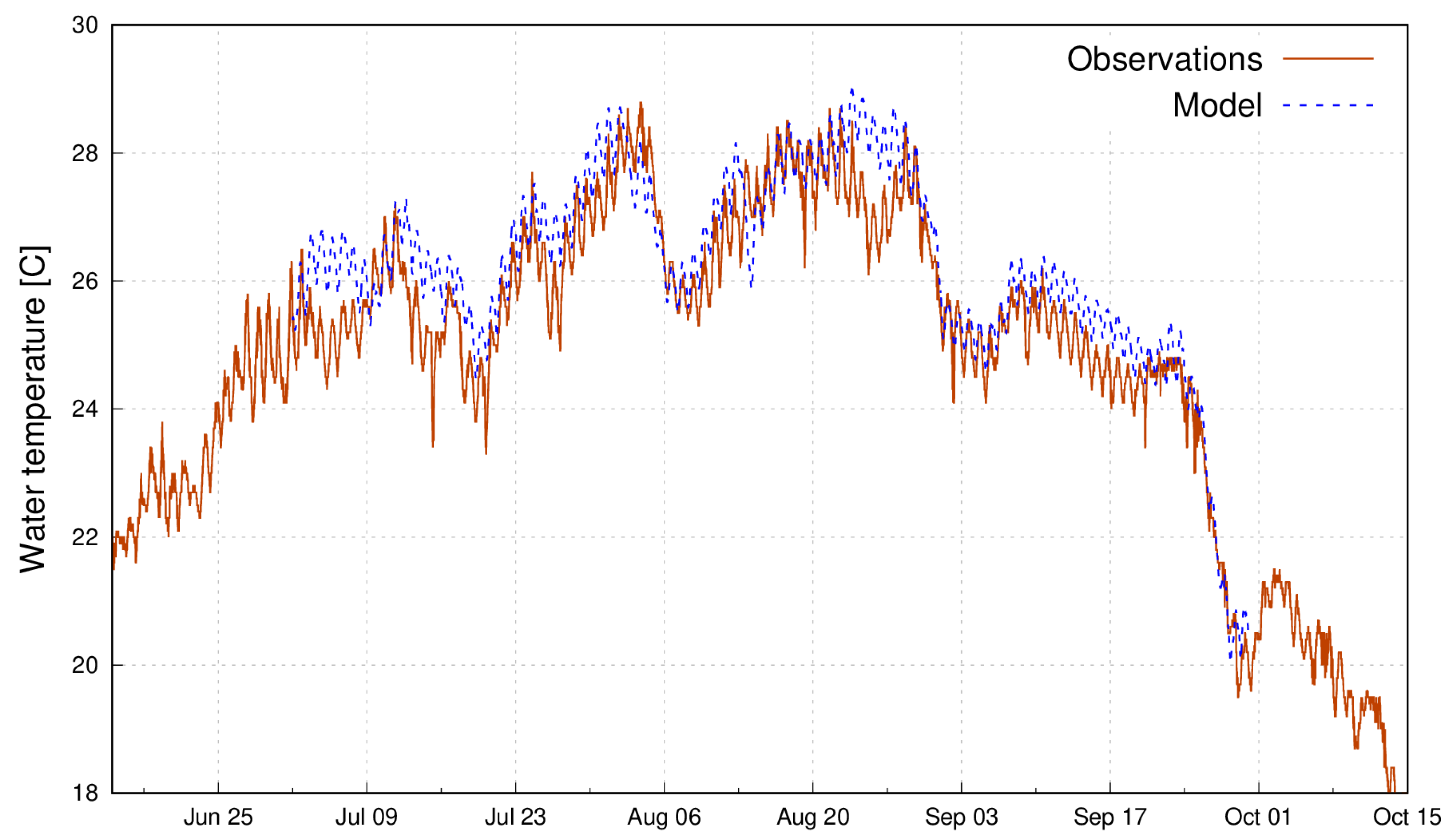
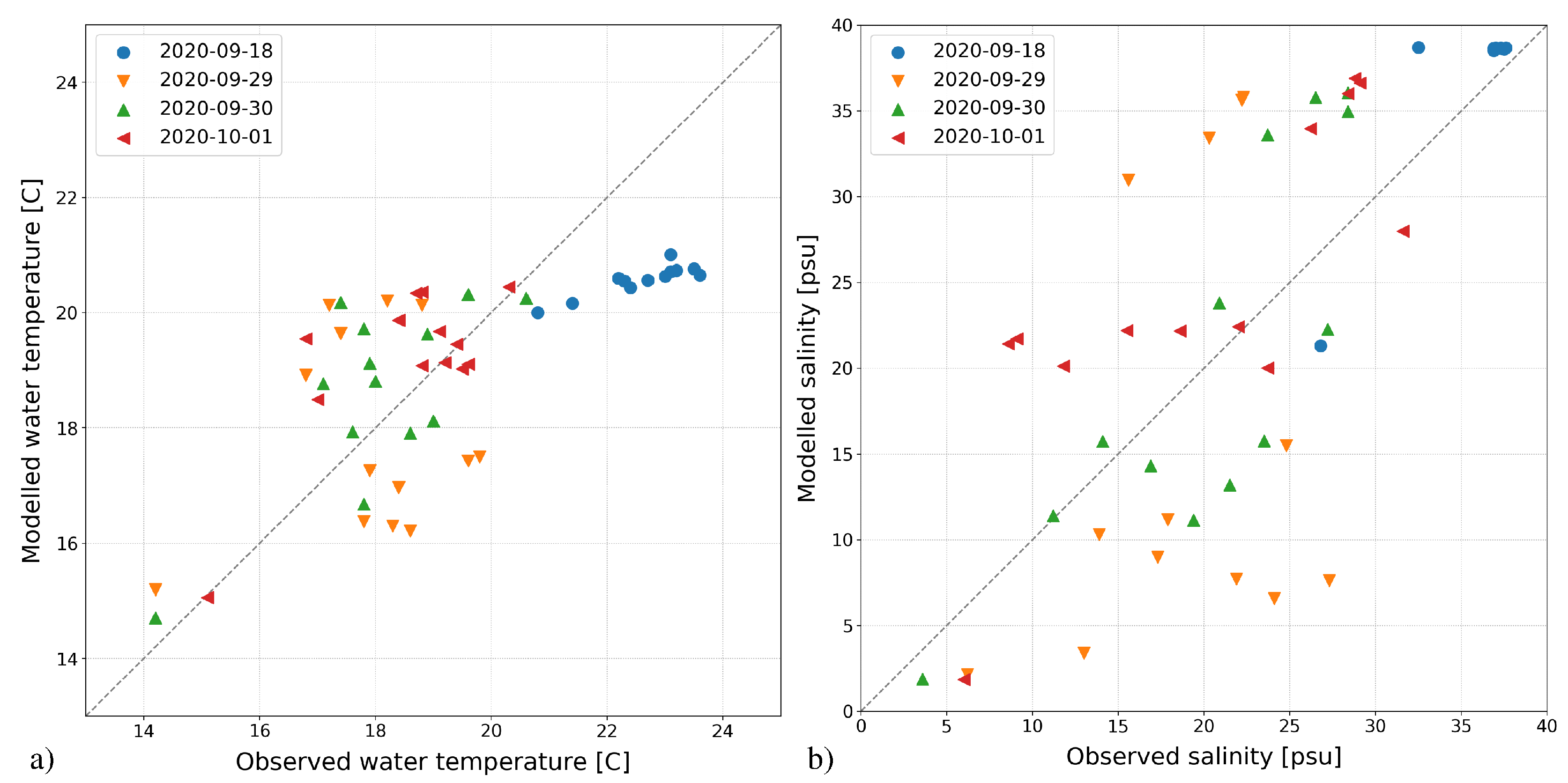
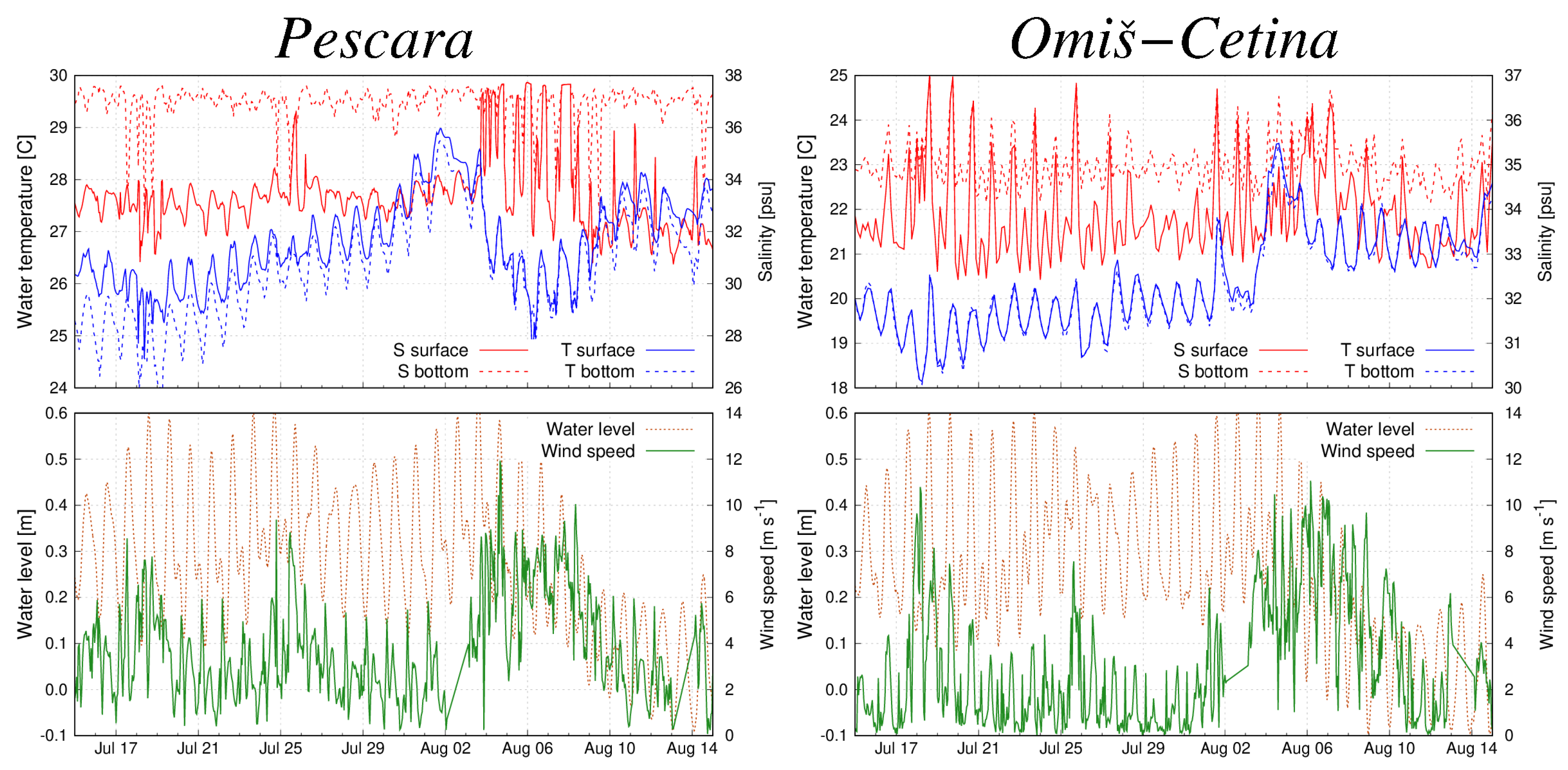
Physicochemical Assessment

The water temperature and salinity values observed in the Fano–Arzilla, Pescara and Raša study areas were used to assess the capacity of the modelling system in reproducing heat fluxes, transport dynamics and mixing processes. Figure 5 shows scatter plots of simulated and observed water temperature (panel a) and salinity (panel b) for the Fano–Arzilla study area. The obtained BIAS and RMSE for salinity are 3.1 and 2.5 psu, and −0.1 ${}^{°}\mathrm{C}$ and 1.2 ${}^{°}\mathrm{C}$ for water temperature. The correlation coefficient resulted to be 0.95 and 0.64 for salinity and water temperature, respectively. The analysis of the results reveals that, despite the large uncertainty on the boundary conditions, the numerical model compares reasonably well with the measurements acquired in Fano coastal waters and reproduces the observed spatial and temporal variability of both water temperature and salinity. The model slightly overestimated salinity.

As shown in Figure 6, model results were generally in good agreement with the continuous water temperature values measured in the Pescara harbour. The model captured the observed weekly variability of the water temperature during the summer of 2020 well, as well as the daily cycle. RMSE, BIAS and R between modelled and observed water temperatures in Pescara are 0.50 ${}^{°}\mathrm{C}$, 0.46 ${}^{°}\mathrm{C}$ and 0.93, demonstrating the good performance of the finite element modelling suite for this study site.

Despite the sparse data and the complexity of the system, the model seems to be able to reproduce the observed salinity and water temperature distributions in the Raša River canal (Figure 7). Salinity ranged from 3 to 38 psu and was generally increasingly moving from the river mouth to the sea, even if during the 18 September 2020 survey, all observations have values around 37 psu. This is due to the temporal fluctuation of the Raša River discharge, which in a few days, passed from less than 1 m${}^3$ s${}^{-1}$ to 15 m${}^3$ s${}^{-1}$ as a consequence of an intense rainy event. The obtained BIAS, RMSE and R for the salinity are 1.3 psu, 7.1 psu and 0.71, and −0.4 ${}^{°}\mathrm{C}$, 1.7 ${}^{°}\mathrm{C}$ and 0.67 for the water temperature. Generally, the model underestimated salinity near the river mouth and overestimated it at the two touristic sites located at 1.5 and 3.4 km from the river mouth. The mismatch could be due to the uncertainty on the bathymetry of the very shallow (less than 1 m) area in front of the river mouth and which was not monitored during the bathymetric survey.

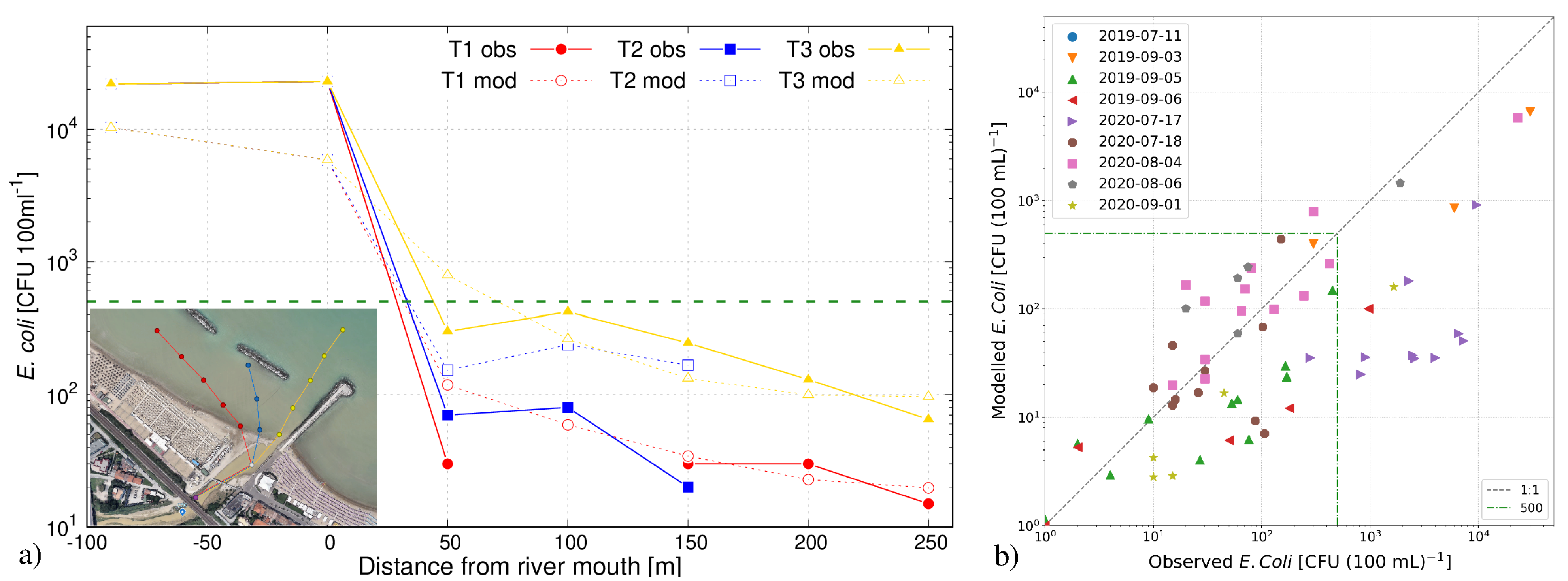
Microbial Pollution Assessment

Regarding microbial pollution, the numerical model results were compared with the E. coli concentration measured in the Fano–Arzilla and Raša study areas for assessing the capacity of the model in reproducing the dispersion and decay of faecal bacteria in nearshore waters. E. coli concentration is reported as CFU 100 mL${}^{-1}$ of water.

In the Fano–Arzilla site, the E. coli concentration was monitored with nine sampling surveys in the summer of 2019 and 2020. More details about the sampling strategy and the microbial analysis can be found in [53]. As shown in Figure 8a, the numerical model provides a realistic representation of the E. coli distribution in the nearshore waters, describing the marked decrease in the bacteria concentration observed from the river mouth towards the open sea. This is mostly due to the effect of dilution with sea waters and decay induced by solar radiation and salinity. According to the scatter plot presented in Figure 8b, the modelling system described (mostly within an order of magnitude precision) the observed E. coli concentration measured in the two years of sampling activity well. RMSLE for E. coli concentration in Fano–Arzilla is 0.18, a value below the ones reported in other studies [7,18,20,56], and the correlation coefficient is 0.93. During some events, e.g., on 5 September 2019 and 17 July 2020, the model underestimated the bacterial concentration in coastal waters. Such discrepancy could be related to the occasional formation of ephemeral stagnant freshwater pools at the river mouth, not reproduced by the model, where bacteria proliferate before reaching the sea.

In the Raša River canal, the model is reproducing the observed E. coli concentrations with a satisfactory agreement (Figure 9a). RMSLE and R for E. coli concentration in Raša are 0.44 and 0.68, respectively. E. coli concentrations at the mouth of the Raša River and adjacent touristic locations were below 10 CFU 100 mL${}^{-1}$ on 18 September 2020 and increased up to the bathing limit of 500 CFU 100 mL${}^{-1}$ as a consequence of the rainfall rain event of 29 September 2020. As shown in Figure 9b, the polluted waters coming from the Raša River tended to flow along the western coast. The model slightly underestimated the faecal bacterial concentration in Trget and Blaz.

3.2. Comparative Analysis of the Adriatic Study Areas

A comparison study between the five study sites was carried out using the numerical model results. The analysis focused on the hydrodynamic characteristics and the quality of the bathing waters. Since this study concerned the contamination of recreational waters, the comparative analysis is based on the model results obtained for the summer of 2020, considered here as a common period of investigation for all study areas. We selected the summer months because they represent the period in which the bathing sites are mostly populated and microbial pollution events have the highest impact.

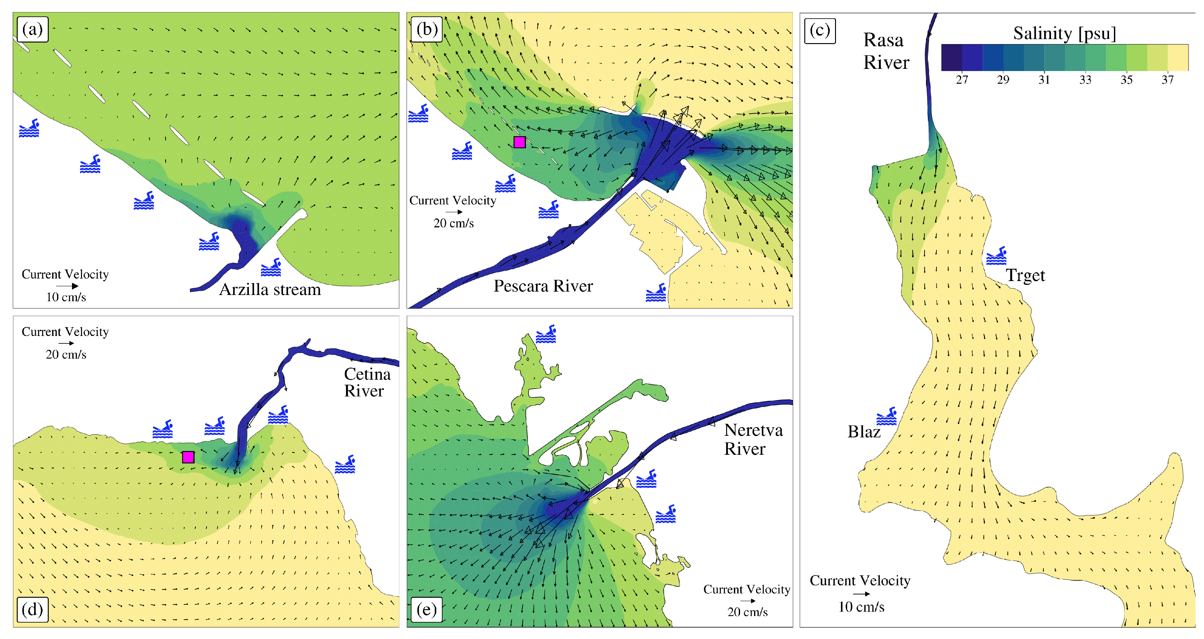
3.2.1. Circulation Dynamics

In this section, we present and compare the hydrodynamic characteristics of the five study areas in terms of current and salinity patterns. The areas of investigation strongly differ for hydraulic and morphological characteristics. They are all coastal areas influenced by freshwater input, which, however, greatly differ for the discharged volumes and seasonal fluctuations. According to the morphological characteristics, we can classify the investigated area in sandy and mild sloping beaches with artificial barriers (Fano and Pescara coasts), gravel/rocky and steep shores (Omiš and Ploče coasts) and semi-enclosed coastal environments (Raša River canal). As a result of such variability and other forcing factors (the main characteristics of which are reported in

Table 3. Characteristics of the main forcing factors (river flow, tidal range, sea temperature and wind speed) in the five study areas.

Study Area	Tidal Range	River Flow	Sea Temperature	Wind Speed
	[m]	[m${}^3$s${}^{-1}$] (Mean/Max)	[${}^{°}\mathbf{C}$] (Mean/Max)	[m s${}^{-1}$] (Mean/Max)
Fano–Arzilla	0.55	0.2/3.7	27/32	2.3/12.8
Pescara	0.34	38.0/60.0	27/29	3.8/12.2
Raša River	0.55	0.8/9.0	23/27	3.1/15.0
Omiš–Cetina	0.37	8.0/9.0	23/27	3.1/17.7
Ploče–Neretva	0.39	200.0/450.0	23/26	3.5/16.3

), the oceanographic conditions of the study sites are driven by different dominant processes which may determine different transport and diffusion dynamics. Salinity can be used as a proxy for the dispersion of contaminated water coming from the rivers.

As a first step, let’s have a look at the main surface circulation and salinity patterns in the different sites (Figure 10). Even if the analysis focused on summer months, when freshwater inputs were at a minimum, generally, the water circulation near the river mouth was mainly driven by the river flow and its interaction with the coastal currents. In the Fano–Arzilla (Figure 10a) and Pescara (Figure 10b) sites, the main circulation resulted in being strongly influenced by the artificial structures (reefs and breakwaters) with the consequent deflection of the riverine waters towards the touristic western beaches. Similarly, the waters coming from the Cetina River tended to be deflected westward by the artificial jetty on the left-hand side of the mouth, thus determining the spread of the freshwater plume along populated beaches (Figure 10d). On the contrary, in the Ploče–Neretva site (Figure 10e), the jetties at the river mouth forced the outflowing freshwater to separate from the coast, thus decreasing the probability that polluted waters were transported to the bathing sites. During stratified summer conditions, the circulation in the Raša River canal was characterized by a surficial layer of water with reduced salinity—due to the freshwater supply—moving towards the open sea, primarily along the eastern side of the fjord (Figure 10c). The strongest surface currents were found in Pescara due to the rather high and constant amount of freshwater discharge by the Pescara River.

Generally, the oceanographic conditions in the Adriatic Sea are characterized by stable thermal stratification in summer [31,57,58]. However, approaching the coast, the vertical stratification of the water column could greatly differ in function of the morphological characteristics and forcing factors. From Simpson and Souza [59], we know that the short-term variability, due to tides and wind, interacts with baroclinic gradients producing vertical variations in the stability of the water column. Indeed, analysing the temporal evolution of the salinity and water temperature fields it emerged that the water column in the investigated coastal areas underwent periodic mixing. In Figure 11, we present the timeseries of surface and bottom water temperature and salinity extracted from the model results in two study areas (Pescara and Omiš–Cetina) near a bathing site at a depth of about 2 m.

Wind and tide concurred in mixing the water column. In Pescara (left panels in Figure 11), the relatively high amount of freshwater stratified the water column (with a 3 psu difference between surface and bottom salinity) and prevented mixing (when bottom water temperature and salinity values equal the surface ones), which occurred only during wind events with speed above 6 m s${}^{-1}$ (e.g., from 4 to 9 August 2020). In Pescara, water mixing was limited by the artificial reef, which confined part of freshwater masses near the beach. Stratification was also favoured by heat fluxes at the water surface. The tidal action modulated the water column stability by enhancing mixing during flood tide through the tidal straining mechanism [60]. Such an effect was more pronounced in the Omiš–Cetina site (right panels in Figure 11), where the water column was fully mixed at a daily frequency. As already noted by [61], spring tides tended to produce well-mixed plumes while neap tides led to stratified plumes. Thermal stratification resulted to be more pronounced on the shallow western coast than the steep eastern shore. Similarly, coastal dynamics in the other study area (not shown) was regulated by wind, freshwater and tide.

Concluding, even if the Adriatic Sea is a micro-tidal environment, the tide is one of the main factors determining mixing in coastal areas [62]. Water mixing, and its variability in time and space, is crucial to be considered due to the dilution of polluted waters and the effect of temperature and salinity on faecal bacterial decay.

3.2.2. Quality of Bathing Waters

The hydrodynamic modelling presented in the previous section is devoted to the description of the water circulation under the influence of different forcing, but many substances are transported within the water. The concurrence of atmospheric forcing, tide and freshwater inflows, led the Adriatic Sea to be characterized by a wide range of different transport phenomena. The analysis of the salinity patterns already provided indications on the transport processes, and also, on the coastal areas mainly influenced by river inputs. However, detailed numerical modelling of faecal bacteria was required for assessing the impact of microbial pollution on the quality of bathing waters.

Recreational waters in the investigated study areas were influenced by different sources of microbial pollution. The water quality in two Fano–Arzilla and Pescara study areas were influenced by urban sewage outfall triggered by heavy rainfall that exceeded the capacity of the sewage systems of urban areas (http://www.portaleacque.salute.gov.it/PortaleAcquePubblico/mappa.do, accessed on 10 May 2021). According to the regular monitoring activities, the three Croatian locations (Raša, Omiš–Cetina and Ploče–Neretva) had an excellent bathing water quality—on the basis of criteria defined by the EU bathing water directive—for the year 2020 (http://baltazar.izor.hr/plazepub/kakvoca/, accessed on 10 May 2021). Potential sources of microbial contamination of coastal waters are polluted river discharges and specific local discharges coming from legal and illegal sewer connectors.

To describe the transport, diffusion and decay of faecal bacteria in coastal waters, the performed simulations accounted for specific pollution events that occurred in the different study areas in summer 2020 and that were detected by the local bathing water management authority. The numerical results were processed to obtain maps of maximum E. coli concentration over the summer 2020 period (Figure 12). Even if limited to a specific year of investigations, the maximum E. coli concentration maps provide clear indications of the zones more affected by microbial pollution.

In the Fano–Arzilla (Figure 12a) and Pescara (Figure 12b) sites, the E. coli plume extends from the river mouth and is constrained by the breakwater and artificial reefs which direct the flow of polluted waters towards the beaches. As a consequence, the nearshore E. coli concentration exceeded the BWD threshold values of 500 CFU 100 mL${}^{-1}$. These two cases represent examples of inadequate planning of coastal defences, which were designed to protect beaches from erosion but have determined a worsening of bathing waters quality. In the Croatian pilot areas, the modelling results revealed for summer 2020 a good water quality at almost all bathing locations of the Croatian study areas, as detected with the monitoring activity. In the Raša River site, E. coli concentration above the BWD threshold can be identified only near the river mouth and the polluted waters did not reach the bathing locations of Trget and Blaz (Figure 12c). Similarly, in the bathing locations of the Omiš–Cetina site (Figure 12d), the E. coli concentration remained below the BWD limit due to the strong dilution of the polluted waters near the river mouth. Figure 12e shows the maximum E. coli concentration in the Ploče–Neretva site with the highest values found in the bay near the city of Ploče due to the discharge of wastewater from local point sources. The untreated waters discharged into the Neretva River at Opuzen and Metković are diluted by the freshwater flow and, consequently, the E. coli contamination from riverine waters had no significant impact on the coastal bathing sites. It has to be noted that only mean values of wastewater discharge were available for the Croatian sites and therefore the real bacterial concentrations can be higher than the simulated ones during intense pollution events.

In addition to the detailed spatial representation of microbial contamination, the numerical model allows for describing the temporal evolution of E. coli concentration during and after a pollution event. As an example, we report in Figure 13 the timeseries of the E. coli concentration at a control station in the Fano–Arzilla site (indicated by the magenta square in Figure 12a; depth of about 1 m) in August 2020 when two heavy rain events (Figure 12b) in succession triggered sewer outflows. E. coli concentration in the coastal waters rose suddenly after the opening of the Arzilla spillway reaching a peak value of 10${}^4$ CFU 100 mL${}^{-1}$, well above the BWD threshold. The concentration remained above the threshold for about 12 h and then decreased to values of about 100 CFU 100 mL${}^{-1}$. The analysis of the timeseries clearly shows that the concentration is strongly modulated by the tidal action (blue line in Figure 12b) with peak values occurring during low tide. Concentrations above the threshold were found for about 3 days after the first rainy event. However, such peaks lasted for only a few hours per day.

Figure 13. Time evolution of the modelled E. coli concentration in the Fano–Arzilla site (at the control station marked with the magenta square in Figure 12a). The bottom panel reports rain and sea level.

Figure 13. Time evolution of the modelled E. coli concentration in the Fano–Arzilla site (at the control station marked with the magenta square in Figure 12a). The bottom panel reports rain and sea level.

As illustrated in Figure 14, E. coli concentration in Raša River promptly responded to a river flood event and then was modulated by the tide, which determined a marked daily oscillation with values varying from 0 to 100 CFU 100 mL${}^{-1}$. The concentration was extracted at a control station located at 400 m from the river mouth and with a mean depth of 2.7 m (magenta square in Figure 12c). Even in such a shallow environment, an estuarine circulation system was present with the polluted riverine waters flowing on the surface. As a result, a strong vertical bacterial concentration is detected, with a two-order of magnitude difference in the bacterial concentration between surface and bottom. Similar results are found in the other investigated study sites, even the one experiencing a small tidal oscillation (not shown for lack of space).

Since E. coli is an allochthonous bacteria in the coastal marine waters that originates from the intestinal tract of humans and other animals, its survival in the marine environment is affected by different environmental factors. Although some authors have pointed to the significant individual and synergistic effects of salinity, turbidity, and vertical interference on E. coli survival [63,64,65], solar radiation still has the highest impact [66]. The analysis of our modelling simulations in the Adriatic Sea confirmed that the solar radiation had the main effect on the survival of E. coli reducing bacteria significantly in marine water (see also Figure 3), concurring with tide in determining the daily oscillations detected at all study sites. Indeed, E. coli peaks presented in Figure 13 and Figure 14 occurred during low tide and nighttime conditions. Salinity and water temperature, as already revealed by the experiments performed by Jozić et al. [66], did not significantly affect the survival of E. coli, and consequently, they had a marginal role in determining the spatial and temporal distribution of the bacteria concentration in coastal waters.

4. Conclusions

This study presents a relocatable coastal water quality prediction model—consisting of hydrodynamic, dispersion and decay modules—that can be used for investigating the spatial and temporal evolution of microbial pollution in coastal ecosystems. The developed water quality model was successfully applied and validated in several coastal areas facing the Adriatic Sea. We summarize our main conclusions and recommendations in the following main points.

• Numerical model results demonstrated that, in the Adriatic Sea, dilution and mixing had a stronger effect on bacteria reduction with respect to microbial decay induced by base mortality, water temperature, salinity and sunlight.
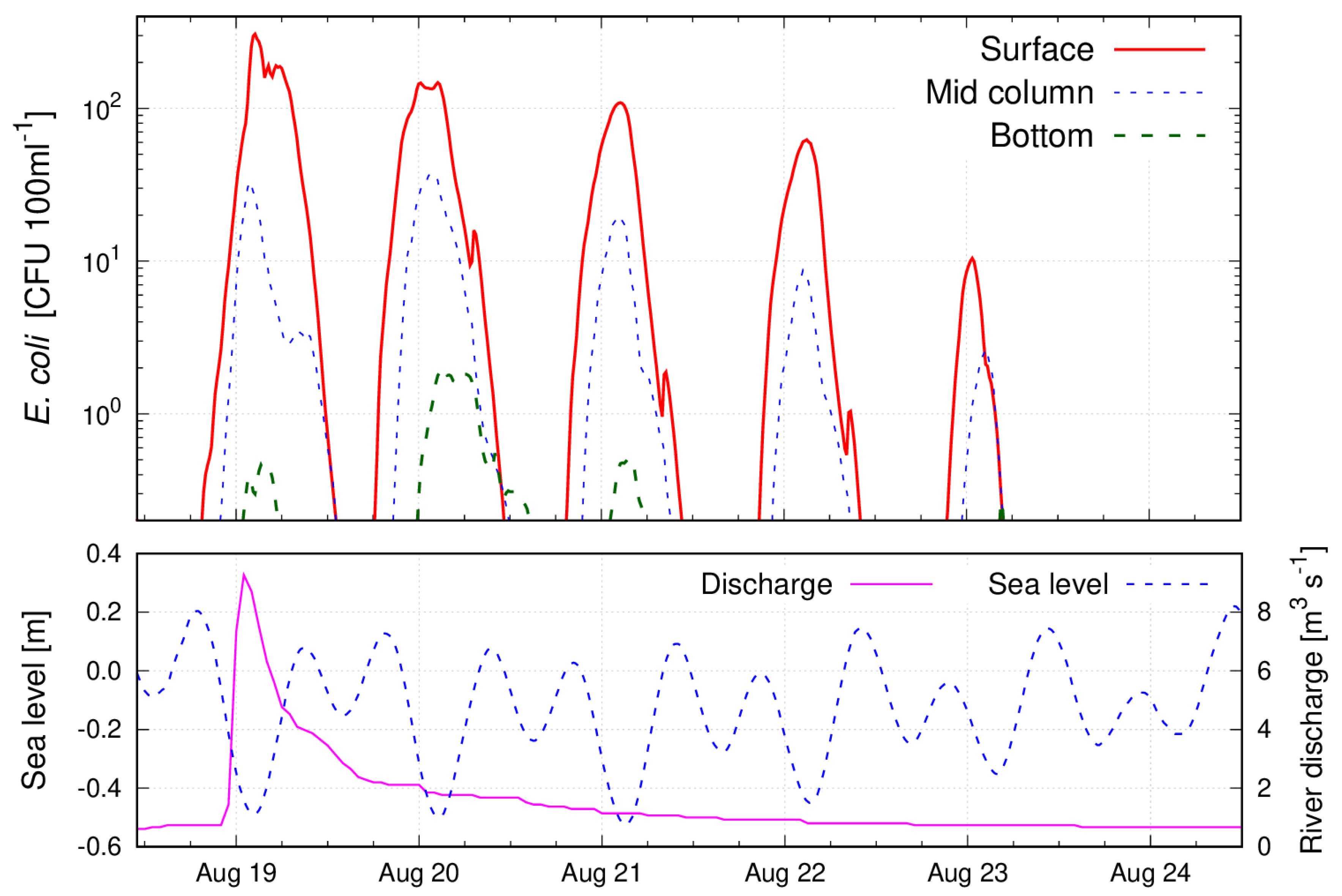
• The estuarine circulation near the river mouth favoured the seaward transport of polluted riverine waters during the decreasing tide and obstructed the river outflow during the rising tide. Due to the thermohaline stratification, strong vertical gradients of bacterial concentration were found at the considered bathing sites.
• The comparative analysis among the different study sites revealed a high spatial and temporal variability of the circulation and dispersion dynamics in coastal waters, which cannot be adequately described by the ordinary monitoring activity that is performed at scheduled intervals in few stations (e.g., in the Fano–Arzilla site, 3 mid-column sampling stations every 15 days during the bathing season).
• The modelling of faecal microbial contamination requires detailed information on input sources from observations for a realistic representation of the bacteria plume in coastal waters. However, the continuous monitoring of bacteria concentration in coastal seas is challenging and a large number of observational sites are required to correctly describe the interactions at the land-sea transition. This is especially true in coastal systems, as the ones investigated in this study, that are characterized by complex small-scale and high-frequency dynamics.
• Even if each numerical model is a partial, simplified and mostly inaccurate representation of the real world, it can be used for complementing the collected information retrieved by the direct microbial monitoring. The synergic use of in situ observations and models allows a reduction of uncertainties in studying coastal waters and improves our knowledge of those regions also leading to further improvements in developing microbial monitoring and modelling techniques. The assimilation of observations into numerical models is a promising approach for increasing the capacity of an observatory to represent the dynamics of coastal systems [67]. Moreover, being the monitoring activity required to investigate the quality of bathing waters very expensive, numerical models—as the one presented in this study—can be very helpful for designing or optimizing monitoring networks (e.g., [68]).

The numerical model described in this study was developed as part of the Water Quality Integrated System (WQIS) proposed in the WATERCARE project (https://www.italy-croatia.eu/web/watercare, accessed on 10 May 2021), an EU Interreg Italy-Croatia project with the objective of reducing the impact of microbial environment contamination in Adriatic bathing waters. WQIS is composed of a real-time hydro-meteorological monitoring network, an automatic refrigerated sampling system, a water quality monitoring network and a forecast operational modelling suite [53]. The model applications described here will be made operational for providing bathing quality forecasts with the aim of helping the management of faecal bacteria pollution in coastal waters. The relocatable modelling suite presented in this study, as well as the whole WQIS, can be easily implemented in other coastal systems.

References

- Mongruel, R.; Vanhoutte-Brunier, A.; Fiandrino, A.; Valette, F.; Ballè-Béganton, J.; Pérez Agúndez, J.A.; Gallai, N.; Derolez, V.; Roussel, S.; Lample, M.; et al. Why, how, and how far should microbiological contamination in a coastal zone be mitigated? An application of the systems approach to the Thau lagoon (France). J. Environ. Manag. 2013, 118, 55–71. [Google Scholar] [CrossRef] [Green Version]
- Schares, G.; Pantchev, N.; Barutzki, D.; Heydorn, A.; Bauer, C.; Conraths, F. Oocysts of Neospora caninum, Hammondia heydorni, Toxoplasma gondii and Hammondia hammondi in faeces collected from dogs in Germany. Int. J. Parasitol. 2005, 35, 1525–1537. [Google Scholar] [CrossRef]
- Botturi, A.; Gozde Ozbayram, E.; Tondera, K.; Gilbert, N.I.; Rouault, P.; Caradot, N.; Gutierrez, O.; Daneshgar, S.; Frison, N.; Akyol, C.; et al. Combined sewer overflows: A critical review on best practice and innovative solutions to mitigate impacts on environment and human health. Crit. Rev. Environ. Sci. Technol. 2020, 1–34. [Google Scholar] [CrossRef]
- Campisano, A.; Ple, J.C.; Muschalla, D.; Pleau, M.; Vanrolleghem, P. Potential and limitations of modern equipment for real time control of urban wastewater systems. Urban Water J. 2013, 10, 300–311. [Google Scholar] [CrossRef]
- Parker, J.; McIntyre, D.; Noble, R. Characterizing fecal contamination in stormwater runoff in coastal North Carolina, USA. Water Res. 2010, 44, 4186–4194. [Google Scholar] [CrossRef] [PubMed]
- Zhang, W.; Wang, J.; Fan, J.; Gao, D.; Ju, H. Effects of rainfall on microbial water quality on Qingdao No. 1 Bathing Beach, China. Mar. Pollut. Bull. 2013, 66, 185–190. [Google Scholar] [CrossRef] [PubMed]
- Locatelli, L.; Russo, B.; Acero Oliete, A.; Sánchez Catalán, J.C.; Martínez-Gomariz, E.; Martínez, M. Modeling of E. coli distribution for hazard assessment of bathing waters affected by combined sewer overflows. Nat. Hazards Earth Syst. Sci. 2020, 20, 1219–1232. [Google Scholar] [CrossRef]
- European Commission. Directive 2006/7/EC of the European Parliament and of the Council of 15 February 2006 concerning the management of bathing water quality and repealing Directive 76/160/EEC. Off. J. Eur. Union 2006, L64, 37–51. [Google Scholar]
- Fernandes, A.M.; Kirshen, P.; Vogel, R.M. Optimal Siting of Regional Fecal Sludge Treatment Facilities: St. Elizabeth, Jamaica. J. Water Resour. Plan. Manag. 2008, 134, 55–63. [Google Scholar] [CrossRef]
- Al Aukidy, M.; Verlicchi, P. Contributions of combined sewer overflows and treated effluents to the bacterial load released into a coastal area. Sci. Total Environ. 2017, 607–608, 483–496. [Google Scholar] [CrossRef] [PubMed]
- Scroccaro, I.; Ostoich, M.; Umgiesser, G.; De Pascalis, F.; Colugnati, L.; Mattassi, G.; Vazzoler, M.; Cuomo, M. Submarine wastewater discharges: Dispersion modelling in the Northern Adriatic Sea. Environ. Sci. Pollut. Res. Int. 2010, 17, 844–855. [Google Scholar] [CrossRef] [PubMed]
- Ostoich, M.; Ghezzo, M.; Umgiesser, G.; Zambon, M.; Tomiato, L.; Ingegneri, F.; Mezzadri, G. Modelling as decision support for the localisation of submarine urban wastewater outfall: Venice lagoon (Italy) as a case study. Environ. Sci. Pollut. Res. Int. 2018, 25, 34306–34318. [Google Scholar] [CrossRef]
- Yaroshenko, I.; Kirsanov, D.; Marjanovic, M.; Lieberzeit, P.A.; Korostynska, O.; Mason, A.; Frau, I.; Legin, A. Real-time water quality monitoring with chemical. Sensors 2020, 20, 3432. [Google Scholar] [CrossRef]
- Sambito, M.; Freni, G. Strategies for improving optimal positioning of quality sensors in urban drainage systems for non-conservative contaminants. Water 2021, 13, 934. [Google Scholar] [CrossRef]
- Cornelis, P.; Givanoudi, S.; Yongabi, D.; Iken, H.; Duwe, S.; Deschaume, O.; Robbens, J.; Dedecker, P.; Bartic, C.; Wübbenhorst, M.; et al. Sensitive and specific detection of E. coli using biomimetic receptors in combination with a modified heat-transfer method. Biosens. Bioelectron. 2019, 136, 97–105. [Google Scholar] [CrossRef] [Green Version]
- Erdem, O.; Saylan, Y.; Cihangir, N.; Denizli, A. Molecularly imprinted nanoparticles based plasmonic sensors for real-time Enterococcus faecalis detection. Biosens. Bioelectron. 2019, 126, 608–614. [Google Scholar] [CrossRef]
- He, Y.; He, Y.; Sen, B.; Li, H.; Li, J.; Zhang, Y.; Zhang, J.; Jiang, S.C.; Wang, G. Storm runoff differentially influences the nutrient concentrations and microbial contamination at two distinct beaches in northern China. Sci. Total Environ. 2019, 663, 400–407. [Google Scholar] [CrossRef]
- Liu, W.C.; Huang, W.C. Modeling the transport and distribution of fecal coliform in a tidal estuary. Sci. Total Environ. 2012, 431, 1–8. [Google Scholar] [CrossRef]
- Palazón, A.; López, I.; Aragonés, L.; Villacampa, Y.; Navarro-González, F. Modelling of Escherichia coli concentrations in bathing water at microtidal coasts. Sci. Total Environ. 2017, 593–594, 173–181. [Google Scholar] [CrossRef] [PubMed] [Green Version]
- Weiskerger, C.J.; Phanikumar, M.S. Numerical Modeling of Microbial Fate and Transport in Natural Waters: Review and Implications for Normal and Extreme Storm Events. Water 2020, 12, 1876. [Google Scholar] [CrossRef]
- Eregno, F.E.; Tryland, I.; Tjomsland, T.; Myrmel, M.; Robertson, L.; Heistad, A. Quantitative microbial risk assessment combined with hydrodynamic modelling to estimate the public health risk associated with bathing after rainfall events. Sci. Total Environ. 2016, 548–549, 270–279. [Google Scholar] [CrossRef] [PubMed]
- Al Mamoon, A.; Keupink, E.; Rahman, M.M.; Eljack, Z.A.; Rahman, A. Sea outfall disposal of stormwater in Doha Bay: Risk assessment based on dispersion modelling. Sci. Total Environ. 2020, 732, 139305. [Google Scholar] [CrossRef]
- Bellafiore, D.; Ferrarin, C.; Maicu, F.; Manfè, G.; Lorenzetti, G.; Umgiesser, G.; Zaggia, L.; Valle-Levinson, A. Saltwater intrusion in a Mediterranean delta under a changing climate. J. Geophys. Res. Oceans 2021, 126, e2020JC016437. [Google Scholar] [CrossRef]
- Zenelaj, R.; Hila, F. Impact of Urban Wastewater Discharges on the Microbiological Pollution of Rivers Debouching into the Adriatic Sea; Rivers and Citizensn; Università del Salento: Lecce, Italy, 2007; pp. 95–105. [Google Scholar]
- Mozetič, P.; Malačič, V.; Turk, V. A case study of sewage discharge in the shallow coastal area of the Northern Adriatic Sea (Gulf of Trieste). Mar. Ecol. 2008, 29, 483–494. [Google Scholar] [CrossRef]
- Ostoich, M.; Aimo, E.; Fassina, D.; Barbaro, J.; Vazzoler, M.; Soccorso, C.; Rossi, C. Biologic impact on the coastal belt of the province of Venice (Italy, Northern Adriatic Sea): Preliminary analysis for the characterization of the bathing water profile. Environ. Sci. Pollut. Res. 2011, 18, 247–259. [Google Scholar] [CrossRef] [PubMed]
- Šolić, M.; Krstulović, N. Presence and survival of Staphylococcus aureus in the coastal area of Split (Adriatic Sea). Mar. Pollut. Bull. 1994, 28, 696–700. [Google Scholar] [CrossRef]
- Stabili, L.; Cavallo, R. Microbial pollution indicators and culturable heterotrophic bacteria in a Mediterranean area (Southern Adriatic Sea Italian coasts). J. Sea Res. 2011, 65, 461–469. [Google Scholar] [CrossRef]
- Liberatore, L.; Murmura, F.; Scarano, A. Bathing water profile in the coastal belt of the province of Pescara (Italy, Central Adriatic Sea). Mar. Pollut. Bull. 2015, 95, 100–106. [Google Scholar] [CrossRef]
- Luna, G.M.; Manini, E.; Turk, V.; Tinta, T.; D’Errico, G.; Baldrighi, E.; Baljak, V.; Buda, D.; Cabrini, M.; Campanelli, A.; et al. Status of faecal pollution in ports: A basin-wide investigation in the Adriatic Sea. Mar. Pollut. Bull. 2019, 147, 219–228. [Google Scholar] [CrossRef] [PubMed]
- Orlić, M.; Gačić, M.; La Violett, P.E. The currents and circulation of the Adriatic Sea. Oceanol. Acta 1992, 15, 109–124. [Google Scholar]
- Marini, M.; Jones, B.H.; Campanelli, A.; Grilli, F.; Lee, C.M. Seasonal variability and Po River plume influence on biochemical properties along western Adriatic coast. J. Geophys. Res. Oceans 2008, 113, C05S90. [Google Scholar] [CrossRef]
- EMODnet Bathymetry Consortium. EMODnet Digital Bathymetry (DTM 2020). 2020. Available online: https://sextant.ifremer.fr/record/bb6a87dd-e579-4036-abe1-e649cea9881a/ (accessed on 10 May 2021).
- Malcangio, D.; Donvito, C.; Ungaro, N. Statistical Analysis of Bathing Water Quality in Puglia Region (Italy). Int. J. Environ. Res. Public Health 2018, 15, 1010. [Google Scholar] [CrossRef] [Green Version]
- Umgiesser, G.; Ferrarin, C.; Cucco, A.; De Pascalis, F.; Bellafiore, D.; Ghezzo, M.; Bajo, M. Comparative hydrodynamics of 10 Mediterranean lagoons by means of numerical modeling. J. Geophys. Res. Oceans 2014, 119, 2212–2226. [Google Scholar] [CrossRef]
- Ferrarin, C.; Bellafiore, D.; Sannino, G.; Bajo, M.; Umgiesser, G. Tidal dynamics in the inter-connected Mediterranean, Marmara, Black and Azov seas. Prog. Oceanogr. 2018, 161, 102–115. [Google Scholar] [CrossRef]
- Bellafiore, D.; Mc Kiver, W.; Ferrarin, C.; Umgiesser, G. The importance of modeling nonhydrostatic processes for dense water reproduction in the southern Adriatic Sea. Ocean Model. 2018, 125, 22–28. [Google Scholar] [CrossRef]
- Ferrarin, C.; Bajo, M.; Bellafiore, D.; Cucco, A.; De Pascalis, F.; Ghezzo, M.; Umgiesser, G. Toward homogenization of Mediterranean lagoons and their loss of hydrodiversity. Geophys. Res. Lett. 2014, 41, 5935–5941. [Google Scholar] [CrossRef]
- Ferrarin, C.; Davolio, S.; Bellafiore, D.; Ghezzo, M.; Maicu, F.; Drofa, O.; Umgiesser, G.; Bajo, M.; De Pascalis, F.; Marguzzi, P.; et al. Cross-scale operational oceanography in the Adriatic Sea. J. Oper. Oceanogr. 2019, 12, 86–103. [Google Scholar] [CrossRef]
- Smagorinsky, J. General circulation experiments with the primitive equations, I. The basic experiment. Mon. Weather Rev. 1963, 91, 99–152. [Google Scholar] [CrossRef]
- Blumberg, A.; Mellor, G.L. A description of a three-dimensional coastal ocean circulation model. In Three-Dimensional Coastal Ocean Models; Heaps, N.S., Ed.; AGU: Washington, DC, USA, 1987; pp. 1–16. [Google Scholar]
- Burchard, H.; Petersen, O. Models of turbulence in the marine environment—A comparative study of two equation turbulence models. J. Mar. Syst. 1999, 21, 29–53. [Google Scholar] [CrossRef]
- Maicu, F.; De Pascalis, F.; Ferrarin, C.; Umgiesser, G. Hydrodynamics of the Po River-Delta-Sea system. J. Geophys. Res. Oceans 2018, 123, 6349–6372. [Google Scholar] [CrossRef]
- Ham, J.M. Measuring evaporation and seepage losses from lagoons used to contain animal waste. Trans. Am. Soc. Agric. Eng. 1999, 48, 1303–1312. [Google Scholar] [CrossRef]
- Chapra, S. Surface Water-Quality Modeling; McGraw-Hill: Boston, MA, USA, 1997; p. 844. [Google Scholar]
- Mancini, J.L. Numerical Estimates of Coliform Mortality Rates under Various Conditions. Water Pollut. Control Fed. 1978, 40, 2477–2484. [Google Scholar]
- Thomann, R.V.; Mueller, J.A. Principles of Surface Water Quality Modeling and Control; Harper Collins: New York, NY, USA, 1987; p. 644. [Google Scholar]
- Feitosa, R.C.; Rosman, P.C.C.; Carvalho, J.L.B.; Cortes, M.B.V.; Wasserman, J.C. Comparative study of fecal bacterial decay models for the simulation of plumes of submarine sewage outfalls. Water Sci. Technol. 2013, 68, 622–631. [Google Scholar] [CrossRef] [PubMed]
- Madani, M.; Seth, R.; Leon, L.F.; Valipour, R.; McCrimmon, C. Three dimensional modelling to assess contributions of major tributaries to fecal microbial pollution of lake St. Clair and Sandpoint Beach. J. Great Lakes Res. 2020, 46, 159–179. [Google Scholar] [CrossRef]
- Davolio, S.; Stocchi, P.; Benetazzo, A.; Bohm, E.; Riminucci, F.; Ravaioli, M.; Li, X.M.; Carniel, S. Exceptional Bora outbreak in winter 2012: Validation and analysis of high-resolution atmospheric model simulations in the northern Adriatic area. Dyn. Atmos. Ocean 2015, 71, 1–20. [Google Scholar] [CrossRef]
- Fairall, C.W.; Bradley, E.F.; Hare, J.E.; Grachev, A.A.; Edson, J.B. Bulk Parameterization of Air-Sea Fluxes: Updates and Verification for the COARE Algorithm. J. Clim. 2003, 16, 571–591. [Google Scholar] [CrossRef]
- Ferrarin, C.; Maicu, F.; Umgiesser, G. The effect of lagoons on Adriatic Sea tidal dynamics. Ocean Model. 2017, 119, 57–71. [Google Scholar] [CrossRef]
- Penna, P.; Baldrighi, E.; Betti, M.; Bolognini, L.; Campanelli, A.; Capellacci, S.; Casabianca, S.; Ferrarin, C.; Giuliani, G.; Grilli, F.; et al. Water quality integrated system: A strategic approach to improve bathing water management. J. Environ. Manag. 2021, submitted. [Google Scholar]
- Krvavica, N.; Ružić, I. Assessment of sea-level rise impacts on salt-wedge intrusion in idealized and Neretva River Estuary. Estuar. Coast. Shelf Sci. 2020, 234, 106638. [Google Scholar] [CrossRef] [Green Version]
- Codiga, D.L. Unified Tidal Analysis and Prediction Using the Utide Matlab Functions; Technical Report 2011-01; Graduate School of Oceanography, University of Rhode Island: Narragansett, RI, USA, 2011. [Google Scholar]
- Thupaki, P.; Phanikumar, M.S.; Beletsky, D.; Schwab, D.J.; Nevers, M.B.; Whitman, R.L. Budget analysis of Escherichia coli at a Southern Lake Michigan Beach. Environ. Sci. Technol. 2010, 44, 1010–1016. [Google Scholar] [CrossRef] [PubMed]
- Marini, M.; Russo, A.; Paschini, E.; Grilli, F.; Campanelli, A. Short-term physical and chemical variations in the bottom water of middle Adriatic depressions. Clim. Res. 2006, 31, 227–237. [Google Scholar] [CrossRef]
- Marini, M.; Grilli, F.; Guarnieri, A.; Jones, B.H.; Klajic, Z.; Pinardi, N.; Sanxhaku, M. Is the southeastern Adriatic Sea coastal strip an eutrophic area? Estuar. Coast. Shelf Sci. 2010, 88, 395–406. [Google Scholar] [CrossRef]
- Simpson, J.H.; Souza, A. Semidiurnal switching of stratification in the region of freshwater influence of the Rhine. J. Geophys. Res. 1995, 100, 7037–7044. [Google Scholar] [CrossRef] [Green Version]
- Simpson, J.H.; Brown, J.; Matthews, J.; Allen, G. Tidal straining, density currents, and stirring in the control of estuarine stratification. Estuaries 1990, 13, 125–132. [Google Scholar] [CrossRef]
- Simpson, J.H.; Bos, W.; Schirmer, F.; Souza, A.; Rippeth, T.; Jones, S.; Hydes, D. Periodic stratification in the rhine ROFI in the North Sea. Oceanol. Acta 1993, 16, 23–32. [Google Scholar]
- Bellafiore, D.; Ferrarin, C.; Braga, F.; Zaggia, L.; Maicu, F.; Lorenzetti, G.; Manfè, G.; Brando, V.; De Pascalis, F. Coastal mixing in multiple-mouth deltas: A case study in the Po Delta, Italy its modeling. Estuar. Coast. Shelf Sci. 2019, 226, 106254. [Google Scholar] [CrossRef] [Green Version]
- Carlucci, A.; Palmer, D. An evaluation of factors affecting the survival of Escherichia coli in sea water. II. Salinity, pH and nutrients. Appl. Microbiol. 1959, 8, 247–250. [Google Scholar] [CrossRef]
- Šolić, M.; Krstulović, N. Separate and combined effects of solar radiation, temperature, salinity and pH on the survival of faecal coliforms in seawater. Mar. Pollut. Bull. 1992, 24, 411–416. [Google Scholar] [CrossRef]
- Alkan, U.; Elliott, D.; Evison, L. Survival of enteric bacteria in relation to simulated solar radiation and other environmental factors in marine waters. Water Res. 1995, 29, 2071–2080. [Google Scholar] [CrossRef]
- Jozić, S.; Morović, M.; Šolić, M.; Krstulović, N.; Ordulj, M. Effect of solar radiation, temperature and salinity on the survival of two different strains of Escherichia coli. Fresenius Environ. Bull. 2014, 23, 1852–1859. [Google Scholar]
- Carrassi, A.; Bocquet, M.; Bertino, L.; Evensen, G. Data assimilation in the geosciences: An overview of methods, issues, and perspectives. Wiley Interdiscip. Rev. Clim. Chang. 2018, 9, e535. [Google Scholar] [CrossRef] [Green Version]
- Ferrarin, C.; Bajo, M.; Umgiesser, G. Model-driven optimization of coastal sea observatories through data assimilation in a finite element hydrodynamic model (SHYFEM v.7_5_65). Geosci. Model. Dev. 2021, 14, 645–659. [Google Scholar] [CrossRef]