
Optimal Return Policies and Micro-Plastics Prevention Based on Environmental Quality Improvement Efforts and Consumer Environmental Awareness


School of Management, Guangzhou University, Guangzhou 510006, China
*
Author to whom correspondence should be addressed.
Water 2021, 13(11), 1537; https://doi.org/10.3390/w13111537
Submission received: 26 April 2021
/
Revised: 20 May 2021
/
Accepted: 24 May 2021
/
Published: 30 May 2021
(This article belongs to the Special Issue Impacts of Anthropogenic Activities on Water Resources and Ecosystem Health: How to Minimize These Impacts?)
Abstract
:Consumers initiating returns online may produce secondary packaging, while most of the packages are produced by plastics. The more products are returned, the more plastics are used. Existing research indicates that the plastic packages can contribute to the micro-plastics pollution of the environment. As consumer environmental awareness (CEA) improves, more and more consumers are willing to pay extra fees to change the materials of packages from plastics to others in order to protect the environment, prompting enterprises to adjust to their return policies. In this context, this paper takes environmental quality improvement effort and the environmental coefficient as decision variables, and compares the manufacturer’s optimal decisions under with and without return policy. Our results show as follows: (1) There is a positive correlation between CEA and environmental quality improvement effort and the environmental coefficient; that is, environmental quality improvement effort and the environmental coefficient increase with an increase in CEA; (2) When CEA is high (), there is a threshold for manufacturers to invest in environmental effort. However, when CEA is low (), regardless of the return policy the manufacturer implements, its profit increases with the promotion of CEA, and when the manufacturer allows consumer returns, the relationship is more obvious; (3) The manufacturer should adopt an appropriate return policy according to the changes in CEA. When CEA is low (), the manufacturer should adopt a without return policy; when CEA is high (), the manufacturer should adopt a full refund () return policy, which is the optimal profit, and increase investment in environmental protection. From the above conclusions, we suggest that the government should increase the publicity of environmental protection, consumers should establish the awareness of green consumption, and enterprises should increase investment in environmental quality improvement to achieve sustainable development.
1. Introduction
E-Business has greatly changed the people’s consuming behaviors and provides a more convenient shopping setting both online and offline for the consumers. In online purchasing, the consumers usually encounter an obvious information uncertainty. Consumers can neither obtain all the information about the products, nor see and touch the products. Therefore, after receiving the purchased products online, consumers may not be satisfied with price changes, product misfit, inconsistency with prior valuation and other factors [1], thus leading to return the products to the resellers [2]. To reduce or ease the disappointment and shopping risks of consumers caused by dissatisfaction with purchased products, many e-commerce companies have formulated different return policies, such as full or partial refunds, return time agreements, and freight instructions, etc. Return policies can reduce the risk of online shopping to a certain extent and increase market demand, but they have also increased the possibility of online returns for consumers. For example, in the Double 11 event held by Alibaba in 2019, the e-commerce platform supported 7 days of no-question returns, resulting in a large number of returns after the event. The online return rate for the Double 11 event reached 7%. Furthermore, when consumers apply for replacement, manufacturers must repackage the returned products (mainly using plastic bags), which caused micro-plastics pollution in the air, water, as well as land, etc., and environmental pollution prevention is paid greater attention by researchers, enterprises and governments. For example. Danilina and Grigoriev [3] studied information provision in environmental policy design. They provided an intuitive algorithm to compute optimal multi-tier information provision policies, both mandatory and voluntary. In Chaudhuri et al. [4], the authors analyzed the potential effects of different sociodemographic factors that are likely to influence WaSH profile development. Ji et al. [5] pointed out that the aggressive CO emission reduction policy could stimulate the development of CCS technology, and the electric power system would still heavily rely on coal resource, while the tough coal-consumption control policy could directly promote regional renewable energy development and electric power structure adjustment.
In the context of countries vigorously promoting green consumption, more and more consumers are paying attention to this micro-plastics environmental pollution prevention issues, and consumers’ environmental awareness is gradually increasing. This awareness is called consumer environmental awareness (CEA) [6]. The BBGM Consumer Report indicates that approximately 51% of Americans are willing to pay more for products with high environmental quality, and 67% believe that this is an important way to purchase products with environmental benefits [7]. The increase in CEA has prompted companies to focus on environmentally friendly products [8]. Moreover, companies produce green products to improve profit [9]. Supply chain members have proposed reducing carbon emissions in forward flows [10,11] and implementing measures to recycle unqualified products [12,13]. The environmental benefits of green and low-carbon products provide consumers with additional utility, and companies producing green and low-carbon products gain a higher market share, corporate reputation and market value. Related studies have begun to use environmental quality effort as a factor for increasing demand [14] and to use the environmental coefficient to measure the environmental protection of enterprise products [15].
There is a great number of studies focusing on the micro-plastics pollution to water, where the main source of micro-plastic is from over-packaging in returned products [16,17,18,19]. Therefore, we attempted to study the optimal return strategy and micro-plastics prevention activities to the water of e-commerce enterprises when consumers have environmental awareness, including efforts to improve environmental quality, the setting of the environmental coefficient, and the change in market demand and return. For simplicity, this paper refers to e-commerce enterprises as “manufacturers”. We thus investigated the following questions:
1. With the increase in CEA, how should manufacturers decide the optimal environmental quality improvement efforts and environmental coefficient?
2. How does the change of CEA affect the profit of manufacturers?
3. How should manufacturers decide the optimal return policy during the change in CEA?
First, we set two variables as the manufacturer’s decision variables (environmental quality improvement efforts and environmental coefficient). The change of CEA affects not only market demand but also the return of consumers. In the process of return, considering CEA, manufacturers will improve packaging, but this improvement will also increase the cost of return, which further leads to more costs for consumers. However, consumers with higher environmental awareness are more willing to pay for environmental protection. Therefore, manufacturers must make their best effort to improve environmental quality and the environmental coefficient to address different levels of consumer environmental awareness.
Second, on the basis of previous studies, we build a manufacturer’s profit function model to better reflect the changes of the manufacturer’s profit. With an increase in CEA, consumers are more willing to pay additional fees for environmental protection in the process of returns. Furthermore, the manufacturer’s return policy will also increase market demand, which will impact the manufacturer’s profit. By calculating the manufacturer’s profit under different policies, we find that the manufacturer’s profit increases with an increase in CEA, and in the case of returns, the change is more obvious. On the one hand, the manufacturer’s return policy increases market demand; on the other hand, it also yields more returns. However, due to the existence of CEA, consumers are willing to pay the cost of returns, so the manufacturer can maximize its revenue according to the change in CEA.
Third, our research divides the manufacturer’s return policy into two types: with return policy and without return policy. To some extent, the return policy alleviates the uncertainty of online purchasing and increases market demand. However, an excessively generous return policy will also hurt corporate income [20]. Therefore, manufacturers must adjust the return policy to achieve their goal of maximizing profit. By calculating and comparing the manufacturer’s profit in two cases, we find that when CEA is low, the manufacturer should adopt a without return policy and reduce the effort and coefficient of environmental quality improvement. By contrast, when CEA is high, the manufacturers should adopt a strategy of returns to improve the effort and coefficient of environmental protection quality improvement. In this scenario, the manufacturer’s income reaches the maximum. However, when CEA reaches a threshold, further increases in environmental quality improvement effort and environmental coefficient are not conducive to increased corporate profit. Therefore, the manufacturer should develop the optimal return policy according to the change in CEA to achieve the goal of maximizing its profit. The government and other relevant departments should actively promote environmental protection, improve the environmental awareness of consumers, urge manufacturers to increase investment in environmental protection packaging, reduce the pollution of secondary packaging, and practice the concept of sustainable development.
The paper is organized as follows: We illustrate the research motivation and questions in Introduction; and review the relevant studies in the following section Literature Review; We then propose the research model and assumptions in Section 3; The model is analyzed and results are discussed through presenting the propositions and corollaries (see Appendix A) in Section 4. We provide a special case study of a full refund return policy in Section 5. Conclusions and discussions are described in the last section.
2. Literature Review
This paper studies a manufacturer’s return policy considering CEA, focusing on the return policy, CEA and environmental quality improvement. Therefore, we review the existing literature related to these three aspects.
2.1. Return Policy
Scholars have done a lot of research on the return problem. Padmanabhan and Png studied the term and method of an enterprise return policy [21], including no return policy, full refund [22,23] and partial refund [24]. In general, consumers have the right to apply for a return to the retailer or manufacturer after purchasing goods [25]. Manufacturers usually adopt the return policies to attract consumers to buy, and a large number of studies show that the return strategy can increase the profits of manufacturers. For example, in direct channels, Su studied how manufacturers adopt a return policy when the consumer valuation is uncertain. The research established a model to compare the manufacturer’s profit under different refund policies and determined the optimal price, refund and order quantity [20]. Hsiao and Chen studied the relationship between product quality risk and return policy: they considered the response of heterogeneous consumers to the return policy. Their research shows that increasing the improvement in product quality does not always yield optimal benefits [1]. Furthermore, Chen and Bell found that in the dual channel, the return policy can increase the manufacturer’s profit [26]. Xu et al. used the newsvendor model to solve the manufacturer’s optimal refund and return deadline and analyzed the possibility of using a return policy to coordinate supply chain benefits [27]. Zhang et al. introduced a two-stage Stackelberg model that allows manufacturers to implement return policies. The results of the study showed that the return policy is beneficial for manufacturers to increase profit when considering consumer utility. In addition, the consumer will prefer manufacturers with return policies when online shopping [28]. Lantz and Hjort [29] and Pei et al. [30] noted that allowing full refunds has a significant positive impact on consumers’ willingness to purchase and increases market demand. Xu et al. showed that the return deadline is positively correlated with consumers’ purchase intention. That is, the longer the return period is, the more willing consumers are to purchase [27].
Most of the previous literature has focused on product quality misfits, refunds, and the purchase behavior of heterogeneous consumers. These studies analyzed how companies adjust the optimal product price and quality to maximize profit; however, they rarely considered the environmental problems caused by returns. In our research, we add the environmental factor into our model.
2.2. Consumer Environmental Awareness (CEA)
Another question is that of how CEA affects manufacturer’s earnings. CEA is also receiving increasing attention from scholars. Previous studies have proven that CEA can indeed improve the performance of enterprises. For example, Conrad studied how CEA affects market share, product attributes and prices [31]. Yakita showed that if CEA is sufficiently high, companies can improve profits by producing green products [32]. The literature on CEA has focused on two areas: product quality improvement and environmental protection policies.
The first area is quality improvement efforts. Quality improvement efforts are seen as a key factor in the supply chain management process [33,34]. For example, Liu et al. and Yu et al. studied how enterprises develop operational strategies under CEA conditions [14,35]. Su noted how zero-sum scenarios and synergy affect the market structure of environmental products [36]. Zhang et al. studied how CEA affects supply chain management and coordination [15]. Ouyang and Fu used mathematical modeling to consider CEA in the energy-sensitive manufacturing industry to study the optimal decisions of enterprises. They concluded that CEA always has a positive impact on the profits of energy enterprises [37].
Another area is environmental protection policy, that is, how the government sets environmental protection strategies to encourage companies to improve the environmental quality of products [38]. Zhang et al. examined how government subsidy strategies affect the design of environmentally friendly products [39]. Luo et al. studied the pricing and emission strategies of two manufacturers with different emission reduction benefits under capped transactions [40]. Furthermore, Zhang et al. studied how the carbon cap trading mechanism affects product design and pricing decisions of competitive manufacturers [41]. Zhang et al. studied the impact of CEA on the order quantity and channel coordination of both retailers and manufacturers. They showed that the retailer’s profit monotonically increases and that the manufacturer’s profit is convex with respect to the CEA [15].
2.3. Environmental Quality Improvement Efforts
Product quality is an important factor to meet the needs of customers and enterprises. Many companies use quality improvement as a powerful competitive tool to fulfill consumer expectations [42]. Xie et al. considered the manufacturer’s improvement in quality at the same price under market segmentation conditions; their results show that the higher the product quality, the greater the market demand [43]. Giri et al. established a supply chain model to study the quality and pricing of multiple oligopoly manufacturers in determining market demand patterns [44]. Chen et al. studied the impact of quality improvement investments on retailers and manufacturers in a dual-channel two-stage supply chain process. They used a Stackelberg game to achieve the optimal quality improvement effort and prices. They found that the retailer can enhance the profit with the improvement of quality. Under different coordination contracts, quality still plays an important role [45]. Reyniers and Tapiero studied the effect of coordinated contracts on supplier quality levels and buyer inspection strategies under cooperative and noncooperative conditions. They further emphasized the importance of contracts and quality management [46]. Lim considered the supplier’s quality improvement strategy in the case of asymmetric information on the basis of predecessors [47]. Zhu et al. considered how to coordinate quality improvement among members in the channel in a single supply chain process [48]. However, the above literature does not consider the cost sharing of quality improvement efforts in the supply chain. This work was eventually completed by [49], who found that greater cooperation should be implemented in the supply chain to improve the level of quality improvement effort. Chakraborty et al. considered the influence of cooperative behavior on channel member pricing and quality improvement decisions in the supply chain. They found that the improvement of quality also increases the supply chain’s profit [50].
The aforementioned literature solves the problem of how manufacturers improve quality under competitive conditions; however, product returns are rarely taken into account. In contrast, this article considers the important factor of environmental protection and attempts to study how manufacturers can make adjustments to environmental quality improvement efforts in direct channels.
2.4. Research Gap
In summary, most of the previous research on CEA focused on manufacturers’ product quality improvement and environmental policies. However, the impact of CEA improvement on corporate return strategies is rarely considered. In contrast to previous studies, (1) this paper considers the manufacturer’s return policy from the perspective of CEA, viewing CEA as an important factor in research; (2) we build the manufacturer’s profit function by setting environmental quality improvement efforts and the environmental coefficient, where environmental quality improvement effort represents the improvement of packaging by the manufacturer and the environmental coefficient measures the environmental degree of enterprises compared with traditional enterprises; (3) we also compare the optimal profit of manufacturers under different return policies and discusses the impact of CEA on the profit of manufacturers.
3. Model
3.1. Model Assumptions
Hypothesis 1 (H1).
Basic conditions. Excessively generous refunds do not optimize supply chain performance [20]. In addition, to confirm the tractability of employing a return policy, the refund price must satisfy [51,52]. Furthermore, in order to ensure the manufacturer is profitable and the rationality of the repairing scenario, the price of the product should be greater than the production cost. Furthermore, the unit repair cost of production for a returned product should be less than the unit cost of production for a new product. That is [53,54].
Hypothesis 2 (H2).
Parameter threshold of CEA. According to the relevant literature, CEA affects the willingness of consumers to pay for environmental protection [55]. To simplify the complexity of the model, this paper assumes that CEA is a random variable following a uniform distribution on ; that is, . When , , indicating that consumers are not willing to pay for environmental protection.
Hypothesis 3 (H3).
Demand function. Suppose that market demand is affected by product price, consumer environmental awareness, environmental quality improvement efforts and other factors and that market demand is a linear function of these factors. Similar to the relevant research in Swami and Shah [56], Dong et al. [57], Wang et al. [58], the demand of the market can be written as follows:
In which is the market’s demand potential, which is independent of product price (p), environmental quality improvement efforts (q) and consumer environmental awareness (). is the price sensitivity parameter representing the sensitivity of market demand to product price (). To avoid complex discussions, we assume that market demand can always be met ().
Furthermore, according to the research in Li et al. [51], a consumer can decide whether to return the product after receiving the product. Hence, the return model is given by the following linear equation:
where R represents the whole returned quantity and u is the potential return quantity, which does not depend on the refund (r), environmental quality improvement efforts (q), environmental coefficient () and CEA () factors. and are the sensitivity of the return quantity to the environmental quality improvement effort and refund, respectively. The environmental coefficient represents the difference between the green manufacturer and the traditional manufacturer in terms of environmental degree. Following Liu et al. [14], we assume . When , the manufacturer is a traditional enterprise.
Hypothesis 4 (H4).
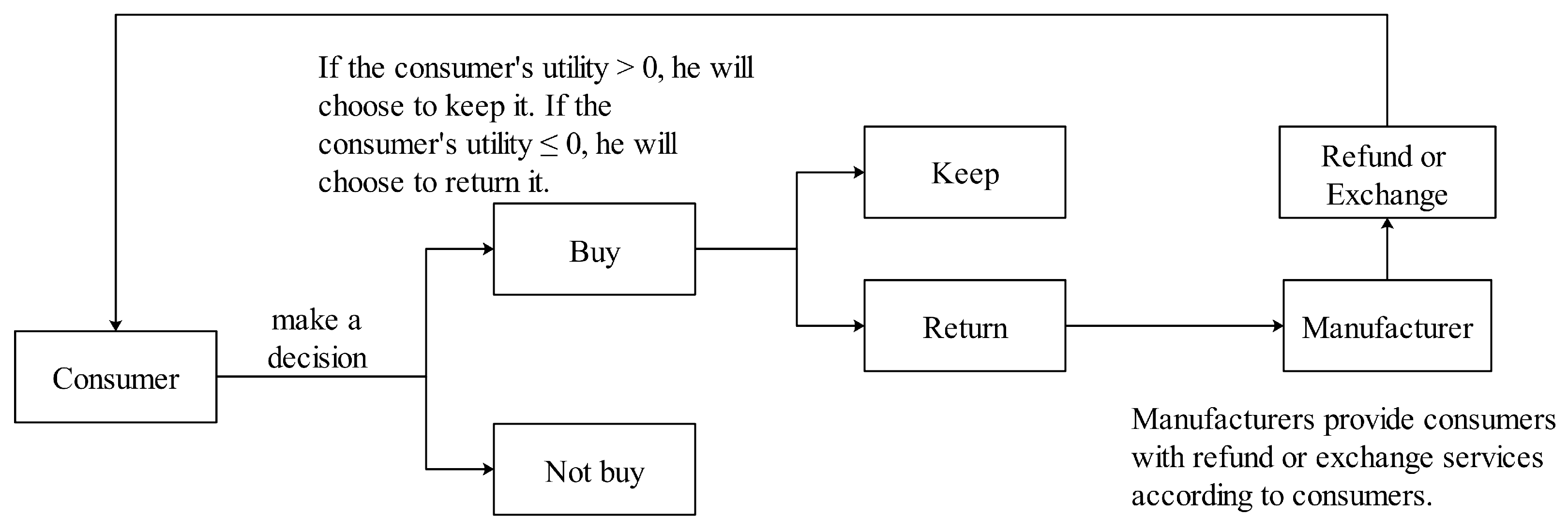
3.2. Consumer
The goal of consumers is to purchase products that meet their expectations. Consumers have two options for returning. One is to choose a refund; that is, the consumer returns the product and receives a certain amount of money. The other is to exchange goods: the consumer returns the product and receives a new product, but this process may require a certain return cost. Whether consumers will return goods depends on whether their utility is satisfied [60]. We use t to represent the proportion of consumers who choose to exchange goods, and represents the proportion of consumers who ask for a refund (). Supposing that consumers have different levels of consumer environmental awareness, a higher level of environmental awareness means that consumers are more willing to pay additional costs for environmental protection during the return process. The specific parameters and variables are shown in Table 1.
Consumer’s purchase process: (a) the consumer considers whether to buy the product; (b) the consumer can choose to keep or return the product after receiving the product; (c) if the consumer chooses to return the product, they can choose a refund or exchange. Manufacturers meet their return needs based on consumer choice. Figure 1 shows the process for consumers to purchase goods.
3.3. Manufacturer
Manufacturers seek to maximize profits and minimize unreasonable returns [1]. Assuming that the manufacturer sets the product’s price p and the refund r [61,62], during the return process, in the face of consumers with different environmental awareness, the manufacturer adjusts its environmental quality improvement effort q and environmental coefficient and implements the optimal return policy to maximize profits. To compare the manufacturer’s profit under different return strategies, we assume that the manufacturer has two return strategies: to accept the consumer’s return application (with return) or to reject the consumer’s return application (without return).
4. Analysis
The manufacturer has two return strategies: reject the return (without return) or accept the return (with return). According to the above assumptions, the profit function of the manufacturer under the two strategies is as follows.
4.1. Without Return Policy
When the manufacturer adopts the without return policy, that is, , , then the manufacturer’s profit function can be written as
where represents the manufacturer’s profit and indicates the direct manufacturer’s revenue at price p. The constraint ensures that market demand is positive. In this paper, we consider only the environmental quality effort, environmental coefficient and packaging cost; we do not focus on price and other product costs.
Lemma 1.
Under the without return policy, when CEA is low (), consumers will not purchase the product. When CEA is high (), consumers will purchase the product when and will not purchase the product when , where
Consumers with different CEA make different purchasing decisions. When a manufacturer implements the without return policy, consumers will be unsure whether the purchased product meets expectations, and since the product cannot be returned, consumers will be more cautious when making a purchasing decision. Therefore, consumers with low CEA will not purchase the product. For customers with high CEA, their purchasing decisions are more affected by product quality improvement efforts. When the product’s environmental quality improvement efforts are high, the consumers will choose to purchase the product.
Proposition 1.
In the case of without return policy, the optimal decision of the manufacturer in equilibrium is , and the manufacturer’s profit is .
According to proposition 1, the partial derivative of the manufacturer’s optimal decision, we have , , . In the case of the no return policy, the manufacturer does not need to consider the issue of consumer returns, so the manufacturer does not need to make greater effort on secondary packaging, that is, . In this scenario, consumers pay more attention to quality, so the manufacturer should improve the product’s quality appropriately.
Corollary 1.
In the case of without return policy, the optimal decision of the manufacturer in equilibrium is , the manufacturer just need to focus on product quality.
Under the policy, according to , , . The lower the packaging cost coefficient is, the higher the manufacturer’s profit. The environmental quality improvement effort q increases with an increase in CEA and decreases with an increase in the coefficient of environmental packaging. Manufacturers can increase profit by increasing the environmental quality improvement effort q and reducing packaging costs.
4.2. With Return Policy
When the manufacturer implements the with return policy, the manufacturer’s return function can be written as
where t represents the proportion of exchanges among returned products. Thus, represents the proportion of requested refunds. indicates the manufacturer’s total refund to consumers. The constraint ensures that the quantity of returns is positive, and ensures that the quantity of returns does not exceed the market demand, which is similar to an actual situation. Additionally, affects the change in market demand and returns and the manufacturer’s profit.
Lemma 2.
Under the with return policy, if CEA is low (), the consumer will purchase the product when a full refund () is available and will not purchase the product in the case of a partial refund (). If CEA is high (), the consumer will choose to purchase the product. Where
Compared with the without return policy, when the manufacturer offers return credit, consumers are more willing to choose to purchase because if the product purchased suffers from quality problems or does not meet expectations, the consumer can choose to return the product. In this scenario, consumers with low CEA are more inclined to request a refund, while consumers with high CEA are willing to pay the additional environmental costs, so they will choose to exchange products.
Proposition 2.
In the case of returns, the optimal decision of the manufacturer in the equilibrium state is as follows: . At this time, the manufacturer’s profit is , where
According to , , when the manufacturer makes a return contract, and are at a high level. Thus, the manufacturer can increase investment in environmental quality improvement effort to respond to the change in CEA.
Corollary 2.
Under the with return policy, and increase with an increase in CEA. The manufacturer should increase the environmental quality improvement effort and environmental coefficient. Moreover, the manufacturer should control the refund because an excessively generous refund strategy () will hurt the manufacturer’s profit.
The higher the value of is, the less sensitive the customer demand is to the return policy and the more sensitive the consumer is to environmental quality. Thus, consumers are more concerned about environmental packaging during the return process: .
The more generous the refund is, the higher the value of and : the refund is positively related to q and . However, an excessively generous refund () will reduce the manufacturer’s profit, according to the equation . Therefore, manufacturers should control the return payment within a reasonable range () for consumers who require a refund while simultaneously increasing environmental quality improvement efforts and environmental coefficient, which can increase market demand.
From Proposition 2, we obtain ; the larger is, the greater the impact on environmental quality improvement efforts. Additionally, the return packaging cost paid by the manufacturer will be higher, which will ultimately decrease the manufacturer’s profit. Manufacturers should choose to increase environmental quality improvement efforts instead of setting excessive refunds. Therefore, in the process of returning, manufacturers should make greater effort in environment quality improvement and reduce the impact of packaging costs, which can increase profit.
According to the above propositions and corollaries, the game between consumers and manufacturers is affected by CEA. The consumer who is not price sensitive but has high environmental awareness should choose a high environmental quality manufacturer that allows returns. Such consumers can be classified as environmentally sensitive. The consumer who is more price sensitive but has weak environmental awareness should choose a manufacturer that allows returns (). Such consumers can be denoted as price sensitive. Both types of consumers prefer a return policy.
4.3. Comparison of Two Return Policies
Table 2 shows that manufacturer’s optimal decision under equilibrium state. The manufacturer’s optimal decision making is different under different return policy conditions. In this part, we further compare the manufacturer’s optimal decision under the without return policy and with return policy.
Lemma 3.
Compared with the without return policy, manufacturers invest more in environmental quality improvement efforts and environmental coefficients under the with return policy, that is: , , where , .
Lemma 3 shows that manufacturers invest more in environmental effort under the condition of a return policy. Because when the manufacturer adopts a without return policy, no consumer will return the product, so . However, under the condition of a return policy, environmentally sensitive consumers affected by CEA are more willing to pay for environmental protection, so manufacturers have to increase investment in environmental protection.
Furthermore, considering that the manufacturer’s return decision is affected by CEA, as CEA increases, the manufacturer’s profit under different return policies are different because if the manufacturer does not allow return, consumers may not purchase the product. Although the manufacturer saves the return cost, both market demand and revenue will decrease. If the manufacturer allows consumers to return the goods online, market demand will increase, but the manufacturer will also face more returns. When the number of returns is too large, the manufacturer must bear considerable return costs, which is also detrimental to the manufacturer’s profit. Therefore, changes in CEA affect the manufacturer’s profit: manufacturers should take an appropriate return policy to achieve their goal of maximizing profit.
Proposition 3.
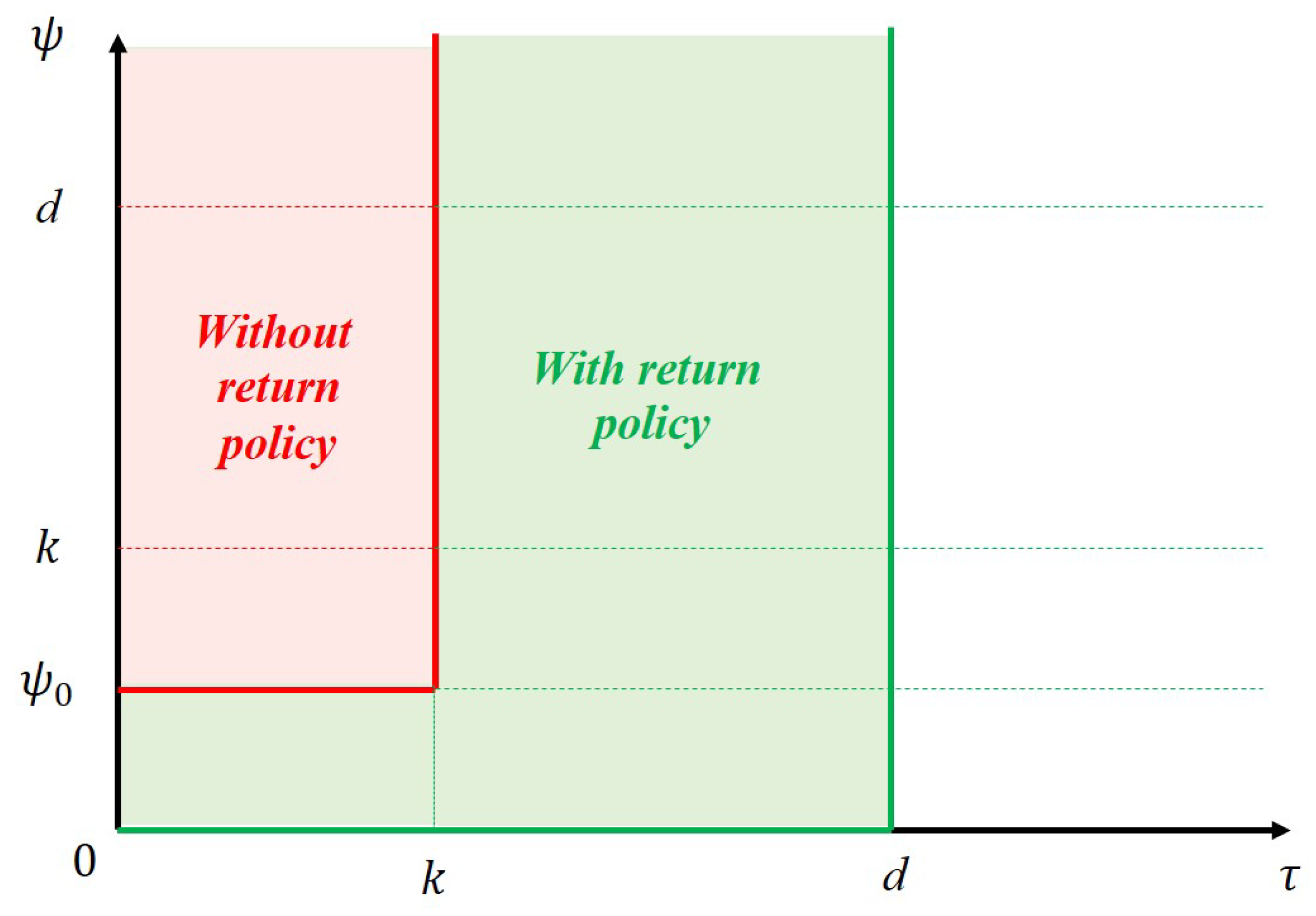
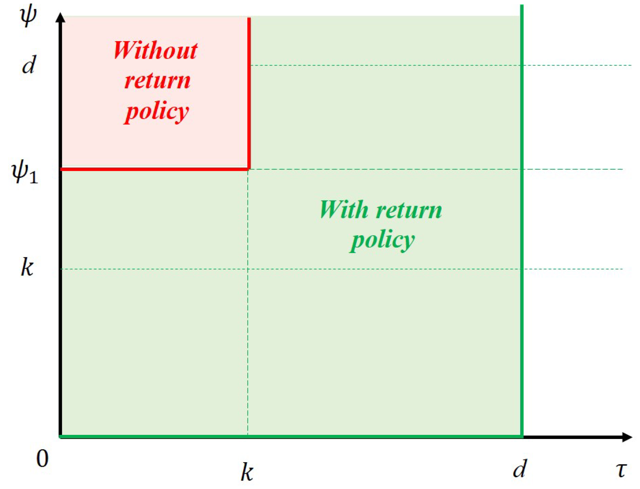
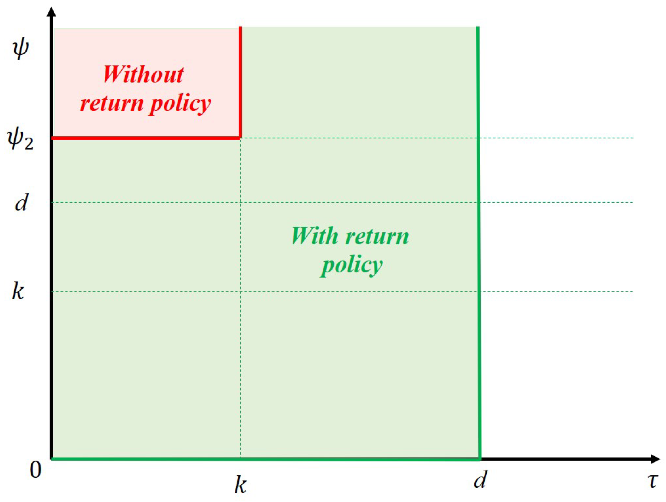
If , then when CEA is low (), . Thus, manufacturers should implement the without return policy. When CEA is high (), , manufacturers should implement the with return policy. If , , the manufacturer should choose the with return policy.
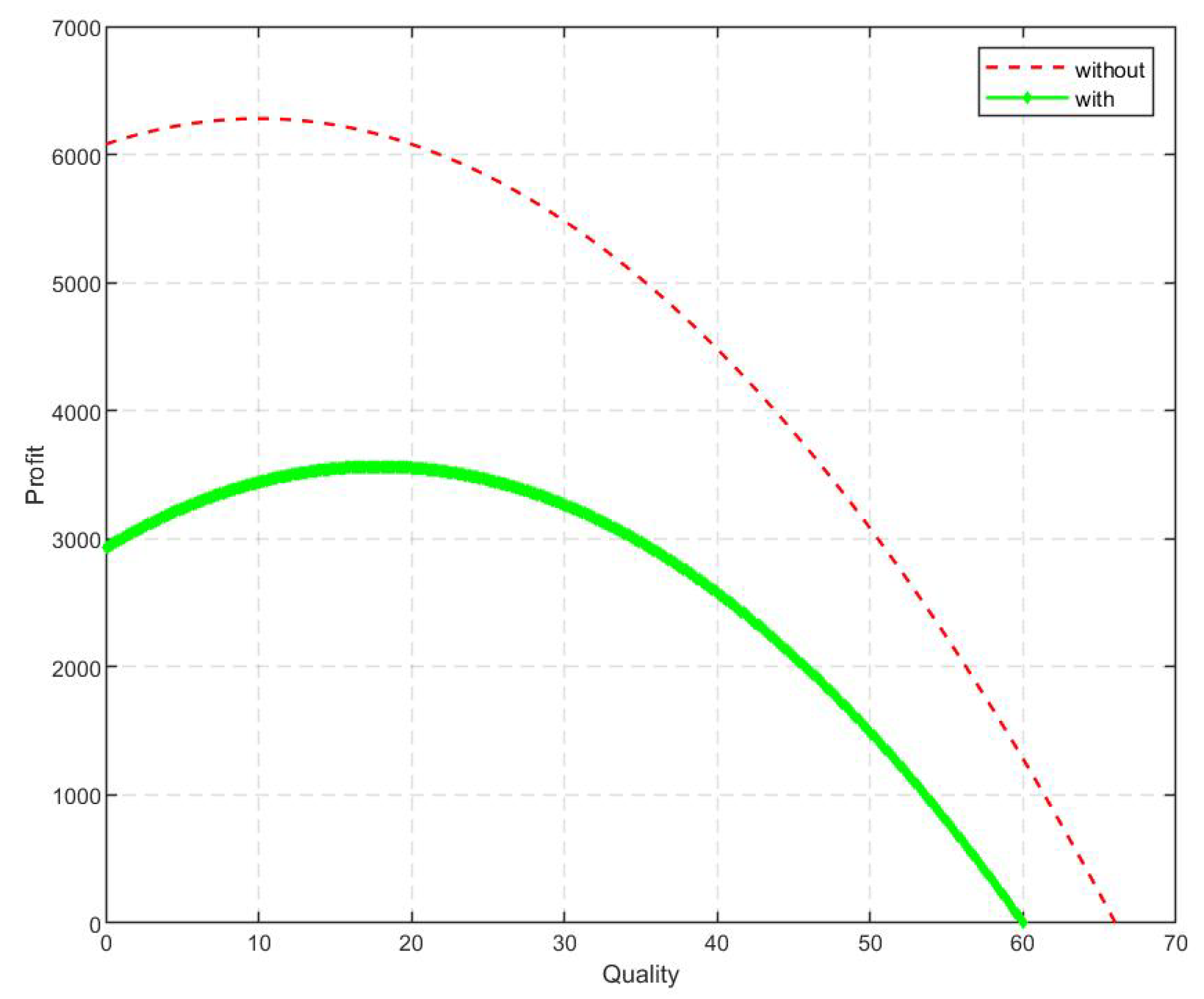
According to Proposition 3, we can draw the manufacturer’s optimal decision diagram as follows, where ; see Figure 2, Figure 3 and Figure 4.
represents the manufacturer’s profit in the case of the with return policy, and represents the manufacturer’s profit in the case of the without return policy. The return policy increases the manufacturer’s profit to a certain extent but does not always optimize revenue. If consumers have low CEA, they are less willing to pay for environmental protection. If the manufacturer implements a return policy at this time, the manufacturer must bear the additional return costs, which will reduce its revenue. As the CEA gradually increases, consumers become more willing to pay for environmental protection, and the profit of the manufacturer increases. Therefore, the manufacturer’s return policy should be adjusted in accordance with changes in CEA.
Corollary 3.
Under the with return policy, and increases as CEA increases. If the cost of improving environmental packaging is low, the manufacturer should increase the environmental quality improvement efforts and environmental coefficient. Furthermore, the manufacturer should control the refund because an excessively generous refund strategy () will hurt the manufacturer’s profit.
According to Proposition 3, when the manufacturer implements a return policy, its profit is higher (), and the profit increases , where .
Faced with consumers who are sensitive to the environment, manufacturers can increase environmental quality improvement efforts to satisfy consumers. At the same time, according to the equation , manufacturers can reduce the refund to prevent consumers from unreasonable returns, especially price-sensitive consumers, who may purchase goods more for the experience and later return the goods, which is detrimental to the manufacturer’s profit.
In the process of return, if the cost of improving environmental packaging is lower, the manufacturer should provide a higher refund and increase investment in environmental protection simultaneously. According to the equation , the lower the value of is, the lower the cost for manufacturers to improve environmentally friendly packaging is. Therefore, manufacturers’ efforts to improve environmental quality will be more attractive to environmentally sensitive consumers.
Manufacturers should distinguish different types of consumers. For price-sensitive consumers, the manufacturer should reduce investment in environmental protection and quality efforts and increase market demand by increasing the refund. For environmentally sensitive consumers, the manufacturer can increase investment in environmental quality efforts and implement a return policy. The reasons are as follows: price-sensitive consumers pay more attention to price issues, and low CEA with has a weak impact on the environment. Therefore, manufacturers can adopt a without return policy without considering consumer returns. When manufacturers implement a with return policy, CEA has a strong positive correlation between quality improvement efforts and environmental coefficients. Meanwhile, manufacturers are facing more possibilities for return, and the cost of returns is gradually increasing. As CEA increases, manufacturers should increase investment in environmental quality improvement efforts to attract more consumers and increase market demand.
4.4. Special Case (r = p)
In this part, we consider the return policy in the case of full refund (). In this scenario, consumer returns depend on environmental quality improvement efforts and environmental coefficients and have no relationship with the return policy. If a consumer’s expectations are not satisfied by a product, the consumer can choose to return the product and receive a full refund. Therefore, the return function should be adjusted as
Similar to the general case, R represents the return quantity. To distinguish between general refund and full refund policies, we use to represent the potential return quantity under the full refund policy, and we suppose .
Hence, the profit function of the manufacturer is as follows:
According to Equation (7), we have the following proposition.
Proposition 4.
Under the condition of a full refund, the manufacturer’s optimal decision is as follows: , and the manufacturer’s profit is , where
According to Proposition 4, in the case of a full refund, , but ; therefore, the environmental quality improvement effort is higher under the full refund policy. Furthermore, the following corollary can be obtained by comparing the full refund and general return policies, where represents environmental quality improvement effort in the case of a full refund.
Corollary 4.
Under the with return policy, and increase as CEA increases. If the cost of improving environmental packaging is low, the manufacturer should increase the environmental quality improvement efforts and environmental coefficient. Furthermore, the manufacturer should control the refund because an excessively generous refund strategy () will hurt the manufacturer’s profit.
Given a range of CEA (), compared with that under the general return policy (), the manufacturer’s profit under the condition of a full refund () is higher; that is, , and the profit increases by .
Where , represents the manufacturer’s profit in the case of a full refund.
Generally, we believe that providing a full refund is not beneficial for the manufacturer’s profit. For example, after purchasing a product, a price-sensitive consumer might request a return if the product does not meet expectations. At this time, the manufacturer must pay a full refund to consumer. If the return quantity is too large, the manufacturer’s actual profits will be reduced. However, according to Corollary 4, the manufacturer’s profit under the full refund is higher than that under the general case. Although the full refund policy may result in a greater number of returns, it is limited to price-sensitive consumers. This strategy also yields increased market demand. For environmentally sensitive consumers, manufacturers can increase their environmental investment to increase their profit because environmentally sensitive consumers are more inclined to choose to exchange products and are willing to pay a fee for environmentally friendly packaging, which ultimately increases the manufacturer’s profit. Corollary 4 modifies our understanding of the partial refund policy ().
4.5. Numerical Example
This paper uses several numerical examples to analyze the changes in the manufacturer’s profit to better demonstrate the above propositions and corollary. Similar to Zhang et al. [15] and Liu et al. [14]. The setting of parameters is consistent with our assumptions and previous research.
Figure 5 shows the relationship between CEA and the manufacturer decision variables when CEA is low (). The parameters are specified as follows: , , , , , , , , , , , . Furthermore, Figure 6 shows the relationship between CEA and the manufacturer decision variables when CEA is high (). The parameters are specified as follows: , , , . We know that when CEA is low, the manufacturer’s profit from the without return policy is greater than that from the return policy. In contrast, when CEA is high, the manufacturer’s profit from the return policy is greater than the profit from the without return policy. This result is consistent with the conclusion of Proposition 3.
5. Discussions
Based on previous study reviews, our research combines current environmental hotspots and studies the issue of returns of e-commerce companies. CEA is included in the consideration of the return policy, and environment-related decision variables are used to measure the manufacturer’s efforts toward environmental protection. This approach expands the existing research on returns. There are some differences between the conclusions drawn in this research and those of previous studies.
In Ouyang and Fu [37] research, they concluded that CEA always has a positive impact on the profits of energy enterprises. However, we found that the manufacturer’s profit is convex with respect to CEA; The reasons for the different conclusions are as follows: (1) The two focus on different products. Ouyang and Fu focus on energy industry products, while this paper focuses on return packaging. (2) The value range of CEA is different. Ouyang and Fu did not consider the impact of low CEA and high CEA. This paper distinguishes consumers with high environmental awareness and low environmental awareness. In fact, CEA cannot increase infinitely, and there is a threshold for CEA. When CEA exceeds this threshold, the profit of manufacturer will not continue to increase. Meanwhile, several managerial implications have been found.
First, manufacturers should classify consumers and adjust environmental quality improvement effort q and environmental coefficient appropriately. Propositions 1 and 2 indicate that environmental quality improvement efforts and the environmental coefficient are affected by CEA. For example, consumers with high CEA () are more willing to pay for environmental protection, so manufacturers can increase investment in environmental quality improvement efforts. By contrast, consumers with low CEA () are more sensitive to price, so manufacturers can correspondingly reduce their investment in environmental quality improvement efforts.
Second, a full refund () yields higher profits than a partial refund (). According to Proposition 3 and Corollary 4, for consumers with high environmental awareness, manufacturers can adopt a partial refund policy () to increase market share. When the manufacturer adopts a full refund policy, its profit is higher than that under the partial refund policy. Every year, during Tmall’s Double Eleven event, both platforms and merchants adopt a 7-day unreasonable return policies, which includes full refund and exchange. This action confirms Proposition 3 and Corollary 4 because manufacturers adopt a full refund policy to expand their market share, and market demand has increased. Consumers do not have to worry about restrictions on returns when purchasing goods, so the manufacturers’ profits increase.
Third, the changes in CEA eventually lead to an equilibrium in the game between consumers and manufacturers. Corollaries 1–3 indicate that changes in CEA can prompt manufacturers to adjust return policy, ultimately affecting the profits of manufacturers. Moreover, manufacturers should make corresponding adjustments based on CEA. If CEA is generally low, manufacturers should reduce the efforts aimed at environmental protection and adopt a without return policy. On the contrary, it is the opposite.
6. Conclusions
This paper examined how a manufacturer adopts optimal return policy by establishing a mathematical model. According to the empirical results, we draw the following three conclusions.
First, CEA has a positive correlation with environmental quality improvement efforts and the environmental coefficient. This relationship is more obvious when the manufacturer allows returns according to Proposition 2. However, when the manufacturer refuses returns, CEA has no effect on the environmental coefficient. In fact, when CEA is low, the manufacturer does not need to increase environmental quality improvement efforts or the environmental coefficient because consumers are not willing to pay extra for environmental protection in this scenario. If the manufacturer invests more in environmental protection, profits will suffer. When CEA is high, manufacturers should increase their investment in environmental protection efforts: an increase in CEA can prompt manufacturers to make adjustments in environmental quality improvement and environmental coefficient.
Second, an increase in CEA has a positive effect on manufacturers’ profits, but the improvement of CEA does not always increase the profits of manufacturers. According to Propositions 1 and 2, Given a suitable range of CEA (), the manufacturer’s profit increases as CEA increases. Furthermore, under the with return policy, CEA has a greater impact on the manufacturer’s profit. However, if CEA is high (), further investment in environmental effort will reduce profits. Although manufacturers increasing investment in environmental efforts will lead to more costs, CEA will not increase indefinitely. Therefore, manufacturers should flexibly adjust their investment in environmental quality.
Third, the manufacturer should adjust the return policy according to changes in CEA. Proposition 3 and Corollary 3 confirm that the manufacturer should adopt a without return policy under low CEA conditions and a with return policy when CEA is high. Although a with return policy can increase market demand, an excessive number of returns will increase the manufacturer’s return cost and reduce the manufacturer’s profit. If CEA is very low, the manufacturer’s return contract will reduce profits because consumers are reluctant to pay extra for environmental protection. If CEA is excessively high, further increases in the environmental quality improvement efforts and environmental coefficient are not conducive to increased profits. Therefore, manufacturers should adjust the optimal return policy according to the changes in CEA to increase profits. Furthermore, we analyzed the manufacturer’s profit under the condition of a full refund (). According to Proposition 4 and Corollary 4, if the manufacturer offers a with return policy, its profit in the full refund scenario is higher than that in the general situation. Therefore, in the case of consumers with the same CEA, manufacturers should choose a full refund return policy.
Obviously, if the CEA is too low, it is not conducive to environmental protection. The key to solving this problem is to increase CEA. Consumers should take the initiative to establish environmental awareness and refuse waste. In addition, state and local governments should actively promote environmental protection and promote circular development and green consumption. Additionally, CEA should be improved through publicity and education. At the same time, environmental protection policies can be issued to relevant companies to prohibit companies from excessively discharging pollution and consuming resources, promote the use of recyclable packaging bags, and reduce excessive packaging to achieve the coordinated development of the economy and environmental protection. In this way, the consumer’s perception of environmental protection can be improved, allowing manufacturers to make further adjustments, such as increasing the use of environmentally friendly packaging and reducing the use of high-polluting materials such as foam and plastic so that the consumer–manufacturer game will reach an equilibrium.
There are some limitations in our study. We considered the return policy in the direct channel, whereas future research can expand the supply chain members by, for example, considering the bilateral channel. Second, this paper assumes that market demand can always be met. In the future, we can consider the choice of return policy under inventory restrictions.
Author Contributions
Authors contributed to this paper equally. All authors have read and agreed to the published version of the manuscript.
Funding
National Natural Science Foudation of China(71801056, 71801059, 71731010, 71802063) and the Humanity and Social Science Youth foundation of the Ministry of Education(18YJC630017).
Institutional Review Board Statement
Not applicable.
Informed Consent Statement
Not applicable.
Data Availability Statement
The data presented in this study are available on request from the corresponding author. The data are not publicly available due to privacy or ethical restrictions.
Acknowledgments
This paper is supported by grants from the National Natural Science Foudation of China(71801056, 71801059, 71731010, 71802063) and the Humanity and Social Science Youth foundation of the Ministry of Education(18YJC630017).
Conflicts of Interest
The authors declare no conflict of interes.
Appendix A
Proof of Proposition 1.
Under the without return policy, that is, , the question can be written as
Then, we can set the Lagrange function , where is the Lagrange multiplier. By differentiating with respect to q, , and and setting the result equal to 0, we can solve this problem using Lagrange’s K-T point method:
To solve these equations, we investigated two cases:
Case 1. it is the K-T point. .
Case 2. Because is less than zero, it is not the K-T point.
To prove that the profit function of the manufacturer is convex, the Hessian matrix of the manufacturer is obtained as
Solving the matrix problem, we have:
Thus, the Hessian matrix is a negative positive definite and has a minimum value. □
Proof of Proposition 2.
Under the with return policy, the question can be written as
Similar to the verification process above, we obtain function L.
where is the Lagrange multiplier. By differentiating with respect to q, , , and and setting the result equal to 0, we can solve this problem using Lagrange’s K-T point method.
To solve these equations, we investigate three cases:
Case 1., it is the K-T point. .
Case 2.. Because is less than zero, it is not the K-T point.
Case 3.. In this case, we need to consider the value of .
- (a)
- When and ,, it is the K-T point; otherwise, it is not the K-T point.
- (b)
- When and , , it is the K-T point; otherwise, it is not the K-T point. In addition,
.
Similar to Proposition 1, to prove that the profit function of the manufacturer is convex, the Hessian matrix of the manufacturer is obtained as
Solving the matrix problem, we have:
Thus, the Hessian matrix is a negative positive definite and has a minimum value. □
Proof of Proposition 3.
According to Proposition 3, the problem can be written as
, and we have .
Then, let .
- (1)
- If , that is, , two cases occur:
- (a)
- When , we obtain the result , that is, .
- (b)
- When , we obtain the result , that is, .
- (2)
- If , that is, , we obtain the result , that is, .
□
Proof of Proposition 4.
When the manufacturer implements the full refund policy, the question can be written as
The solution of the above equation is similar to that of Proposition 2:
(1) , it is the K-T point.
.
The Hessian matrix of the model is similar to that of Proposition 2. □
Proof of Corollary 4
According to Proposition 2 and Proposition 4, we obtain the manufacturer’s optimal profit under a general return policy and a full refund policy. The difference between the two values is as follows:
Let , we obtain:
where represents the profit under a full refund and represents the general profit. The result shows . □
All the Propositions and Corollaries have been proven.
References
- Hsiao, L.; Chen, Y.J. Returns policy and quality risk in e-business. Prod. Oper. Manag. 2012, 21, 489–503. [Google Scholar] [CrossRef]
- Nasiry, J.; Popescu, I. Advance selling when consumers regret. Manag. Sci. 2012, 58, 1160–1177. [Google Scholar] [CrossRef] [Green Version]
- Danilina, V.; Grigoriev, A. Information Provision in Environmental Policy Design. J. Environ. Inform. 2020, 36, 1–10. [Google Scholar] [CrossRef]
- Chaudhuri, S.; Roy, M.; Jain, A. Appraisal of WaSH (Water-Sanitation-Hygiene) Infrastructure using a Composite Index, Spatial Algorithms and Sociodemographic Correlates in Rural India. Environ. Inform. 2020, 35, 1–22. [Google Scholar] [CrossRef]
- Ji, L.; Huang, G.; Niu, D.; Cai, Y.; Yin, J. A Stochastic Optimization Model for Carbon-Emission Reduction Investment and Sustainable Energy Planning under Cost-Risk Control. J. Environ. Inform. 2020, 36, 107–118. [Google Scholar] [CrossRef]
- Ibanez, L.; Grolleau, G. Can ecolabeling schemes preserve the environment? Environ. Resour. Econ. 2008, 40, 233–249. [Google Scholar] [CrossRef]
- Bemporad, R.; Baranowski, M. Conscious consumers are changing the rules of marketing. Highlights from the BBGM Conscious Consumer Report. 2007, pp. 1–6. Available online: http://www.bbgm.com (accessed on 15 July 2019).
- Rahmani, K.; Yavari, M. Pricing policies for a dual-channel green supply chain under demand disruptions. Comput. Ind. Eng. 2019, 127, 493–510. [Google Scholar] [CrossRef]
- Li, B.; Zhu, M.; Jiang, Y.; Li, Z. Pricing policies of a competitive dual-channel green supply chain. J. Clean. Prod. 2016, 112, 2029–2042. [Google Scholar] [CrossRef]
- Govindan, K.; Azevedo, S.G.; Carvalho, H.; Cruz–Machado, V. Impact of supply chain management practices on sustainability. J. Clean. Prod. 2014, 85, 212–225. [Google Scholar] [CrossRef]
- Taleizadeh, A.A.; Alizadeh-Basban, N.; Sarker, B.R. Coordinated contracts in a two-echelon green supply chain considering pricing strategy. Comput. Ind. Eng. 2018, 124, 249–275. [Google Scholar] [CrossRef]
- Mukhopadhyay, S.K.; Ma, H. Joint procurement and production decisions in remanufacturing under quality and demand uncertainty. Int. J. Prod. Econ. 2009, 120, 5–17. [Google Scholar] [CrossRef]
- Xu, L.; Wang, C. Sustainable manufacturing in a closed-loop supply chain considering emission reduction and remanufacturing. Resour. Conserv. Recycl. 2018, 131, 297–304. [Google Scholar] [CrossRef]
- Liu, Z.L.; Anderson, T.D.; Cruz, J.M. Consumer environmental awareness and competition in two- stage supply chains. Eur. J. Oper. Res. 2012, 218, 602–613. [Google Scholar] [CrossRef]
- Zhang, L.; Wang, J.; You, J. Consumer environmental awareness and channel coordination with two substitutable products. Eur. J. Oper. Res. 2015, 241, 63–73. [Google Scholar] [CrossRef]
- Zhang, D.; Fraser, M.A.H.W. Microplastic pollution in water, sediment, and specific tissues of crayfish (Procambarus clarkii) within two different breeding modes in Jianli, Hubei province, China. Environ. Pollut. 2021, 272, 115939. [Google Scholar] [CrossRef] [PubMed]
- Li, Y.; Zhang, Y.; Chen, G.; Xu, K.; Gong, H.; Huang, K.; Yan, M.; Wang, J. Microplastics in Surface Waters and Sediments from Guangdong Coastal Areas, South China. Sustainability 2021, 13, 2691. [Google Scholar] [CrossRef]
- Smyth, K.; Drake, J.; Li, Y.; Rochman, C.; Passeport, E. Bioretention cells remove microplastics from urban stormwater. Water Res. 2020, 191, 116785. [Google Scholar] [CrossRef] [PubMed]
- Li, Y.; Lu, Z.; Zheng, H.; Wang, J.; Chen, C. Microplastics in surface water and sediments of Chongming Island in the Yangtze Estuary, China. Environ. Sci. Eur. 2020, 32, 1–12. [Google Scholar] [CrossRef] [Green Version]
- Su, X. Consumer returns policies and supply chain performance. Manuf. Serv. Oper. Manag. 2009, 11, 595–612. [Google Scholar] [CrossRef] [Green Version]
- Padmanabhan, V.; Png, I.P. Returns policies: Make money by making good. Sloan Manag. Rev. 1995, 37, 65. [Google Scholar]
- Davis, S.; Gerstner, E.; Hagerty, M. Money back guarantees in retailing: Matching products to consumer tastes. J. Retail. 1995, 71, 7–22. [Google Scholar] [CrossRef]
- Che, Y.K. Customer return policies for experience goods. J. Ind. Econ. 1996, 44, 17–24. [Google Scholar] [CrossRef] [Green Version]
- Chu, W.; Gerstner, E.; Hess, J.D. Managing dissatisfaction: How to decrease customer opportunism by partial refunds. J. Serv. Res. 1998, 1, 140–155. [Google Scholar] [CrossRef]
- Mostard, J.; Teunter, R. The newsboy problem with resalable returns: A single period model and case study. Eur. J. Oper. Res. 2006, 169, 81–96. [Google Scholar] [CrossRef]
- Chen, J.; Bell, P.C. Implementing market segmentation using full-refund and no-refund customer returns policies in a dual-channel supply chain structure. Int. J. Prod. Econ. 2012, 136, 56–66. [Google Scholar] [CrossRef]
- Xu, L.; Li, Y.; Govindan, K.; Xu, X. Consumer returns policies with endogenous deadline and supply chain coordination. Eur. J. Oper. Res. 2015, 242, 88–99. [Google Scholar] [CrossRef]
- Zhang, R.; Li, J.; Huang, Z.; Liu, B. Return strategies and online product customization in a dual-channel supply chain. Sustainability 2019, 11, 3482. [Google Scholar] [CrossRef] [Green Version]
- Lantz, B.; Hjort, K. Real e-customer behavioural responses to free delivery and free returns. Electron. Commer. Res. 2013, 13, 183–198. [Google Scholar] [CrossRef]
- Pei, Z.; Paswan, A.; Yan, R. E-tailer? s return policy, consumer? s perception of return policy fairness and purchase intention. J. Retail. Consum. Serv. 2014, 21, 249–257. [Google Scholar] [CrossRef]
- Conrad, K. Price competition and product differentiation when consumers care for the environment. Environ. Resour. Econ. 2005, 31, 1–19. [Google Scholar] [CrossRef]
- Yakita, A. Technology choice and environmental awareness in a trade and environment context. Aust. Econ. Pap. 2009, 48, 270–279. [Google Scholar] [CrossRef]
- Rong, A.; Akkerman, R.; Grunow, M. An optimization approach for managing fresh food quality throughout the supply chain. Int. J. Prod. Econ. 2011, 131, 421–429. [Google Scholar] [CrossRef]
- Bernstein, F.; Federgruen, A. Coordination mechanisms for supply chains under price and service competition. Manuf. Serv. Oper. Manag. 2007, 9, 242–262. [Google Scholar] [CrossRef] [Green Version]
- Yu, Y.; Han, X.; Hu, G. Optimal production for manufacturers considering consumer environmental awareness and green subsidies. Int. J. Prod. Econ. 2016, 182, 397–408. [Google Scholar] [CrossRef] [Green Version]
- Su, J.C.; Wang, L.; Ho, J.C. The impacts of technology evolution on market structure for green products. Math. Comput. Model. 2012, 55, 1381–1400. [Google Scholar] [CrossRef]
- Ouyang, J.; Fu, J. Optimal strategies of improving energy efficiency for an energy-intensive manufacturer considering consumer environmental awareness. Int. J. Prod. Res. 2020, 58, 1017–1033. [Google Scholar] [CrossRef]
- Hammami, R.; Nouira, I.; Frein, Y. Effects of customers’ environmental awareness and environmental regulations on the emission intensity and price of a product. Decis. Sci. 2018, 49, 1116–1155. [Google Scholar] [CrossRef]
- Zhang, X.; Xu, X.; He, P. New product design strategies with subsidy policies. J. Syst. Sci. Syst. Eng. 2012, 21, 356–371. [Google Scholar] [CrossRef]
- Luo, Z.; Chen, X.; Wang, X. The role of co-opetition in low carbon manufacturing. Eur. J. Oper. Res. 2016, 253, 392–403. [Google Scholar] [CrossRef] [Green Version]
- Zhang, L.; Zhou, H.; Liu, Y.; Lu, R. The optimal carbon emission reduction and prices with cap and trade mechanism and competition. Int. J. Environ. Res. Public Health 2018, 15, 2570. [Google Scholar] [CrossRef] [PubMed] [Green Version]
- He, Y.; Xu, Q.; Xu, B.; Wu, P. Supply chain coordination in quality improvement with reference effects. J. Oper. Res. Soc. 2016, 67, 1158–1168. [Google Scholar] [CrossRef]
- Xie, G.; Wang, S.; Lai, K.K. Quality improvement in competing supply chains. Int. J. Prod. Econ. 2011, 134, 262–270. [Google Scholar] [CrossRef]
- Giri, B.; Chakraborty, A.; Maiti, T. Quality and pricing decisions in a two-echelon supply chain under multi-manufacturer competition. Int. J. Adv. Manuf. Technol. 2015, 78, 1927–1941. [Google Scholar] [CrossRef]
- Chen, J.; Liang, L.; Yao, D.Q.; Sun, S. Price and quality decisions in dual-channel supply chains. Eur. J. Oper. Res. 2017, 259, 935–948. [Google Scholar] [CrossRef]
- Reyniers, D.J.; Tapiero, C.S. The delivery and control of quality in supplier-producer contracts. Manag. Sci. 1995, 41, 1581–1589. [Google Scholar] [CrossRef]
- Lim, W.S. Producer-supplier contracts with incomplete information. Manag. Sci. 2001, 47, 709–715. [Google Scholar] [CrossRef]
- Zhu, K.; Zhang, R.Q.; Tsung, F. Pushing quality improvement along supply chains. Manag. Sci. 2007, 53, 421–436. [Google Scholar] [CrossRef]
- Chao, G.H.; Iravani, S.M.; Savaskan, R.C. Quality improvement incentives and product recall cost sharing contracts. Manag. Sci. 2009, 55, 1122–1138. [Google Scholar] [CrossRef] [Green Version]
- Chakraborty, T.; Chauhan, S.S.; Ouhimmou, M. Cost-sharing mechanism for product quality improvement in a supply chain under competition. Int. J. Prod. Econ. 2019, 208, 566–587. [Google Scholar] [CrossRef]
- Li, Y.; Xu, L.; Li, D. Examining relationships between the return policy, product quality, and pricing strategy in online direct selling. Int. J. Prod. Econ. 2013, 144, 451–460. [Google Scholar] [CrossRef]
- Mukhopadhyay, S.K.; Setoputro, R. Reverse logistics in e-business:Optimal price and return policy. Int. J. Phys. Distrib. Logist. Manag. 2004, 34, 70–89. [Google Scholar] [CrossRef]
- Hafezalkotob, A. Competition, cooperation, and coopetition of green supply chains under regulations on energy saving levels. Transp. Res. Part E Logist. Transp. Rev. 2017, 97, 228–250. [Google Scholar] [CrossRef]
- Wu, C.H. Product-design and pricing strategies with remanufacturing. Eur. J. Oper. Res. 2012, 222, 204–215. [Google Scholar] [CrossRef]
- Chitra, K. In search of the green consumers: A perceptual study. J. Serv. Res. 2007, 7, 173–191. [Google Scholar]
- Swami, S.; Shah, J. Channel coordination in green supply chain management. J. Oper. Res. Soc. 2013, 64, 336–351. [Google Scholar] [CrossRef]
- Dong, C.; Shen, B.; Chow, P.S.; Yang, L.; Ng, C.T. Sustainability investment under cap-and-trade regulation. Ann. Oper. Res. 2016, 240, 509–531. [Google Scholar] [CrossRef]
- Wang, Q.; Zhao, D.; He, L. Contracting emission reduction for supply chains considering market low-carbon preference. J. Clean. Prod. 2016, 120, 72–84. [Google Scholar] [CrossRef]
- Ji, J.; Zhang, Z.; Yang, L. Carbon emission reduction decisions in the retail-/dual- channel supply chain with consumers’ preference. J. Clean. Prod. 2017, 141, 852–867. [Google Scholar] [CrossRef]
- Chen, Y.; Wang, D.; Chen, K.; Zha, Y.; Bi, G. Optimal pricing and availability strategy of a bike-sharing firm with time-sensitive customers. J. Clean. Prod. 2019, 228, 208–221. [Google Scholar] [CrossRef]
- Xu, X.; Chen, Y.; He, P.; Yu, Y.; Bi, G. The selection of marketplace mode and reselling mode with demand disruptions under cap-and-trade regulation. Int. J. Prod. Res. 2021, 1–20. [Google Scholar] [CrossRef]
- Chen, Y.; Zha, Y.; Wang, D.; Li, H.; Bi, G. Optimal pricing strategy of a bike-sharing firm in the presence of customers with convenience perceptions. J. Clean. Prod. 2020, 253, 119905. [Google Scholar] [CrossRef]
Figure 1.
Consumer purchase process.

Figure 2.
Manufacturer’s optimal decision ().

Figure 3.
Manufacturer’s optimal decision ().

Figure 4.
Manufacturer’s optimal decision ().

Figure 5.
Manufacturer’s profit comparisons ().

Figure 6.
Manufacturer’s profit comparisons ().


Table 1.
Model parameters and decision variables.
| Parameters | |
|---|---|
| p | Price per unit of product |
| c | The unit cost of production for new product |
| The unit repair cost of production for returned product | |
| r | Refund for unit product paid by the manufacturer |
| Consumer environmental awareness () | |
| t | Rate of exchange among returned products |
| e | Fixed packaging cost |
| Potential market demand | |
| Price sensitivity parameter representing the sensitivity of demand to the selling price | |
| u | Based return quantity |
| Sensitivity of the return quantity to quality | |
| Sensitivity of the return quantity to refund | |
| Fixed investment coefficient of the quality improvement effort | |
| Decision variables | |
| q | Environmental quality improvement effort |
| Environmental coefficient | |
| Performance indicator | |
| Profit of the manufacturer | |
| Profit of the manufacturer without return policy | |
| Profit of the manufacturer under general return policy | |
| Profit of the manufacturer under full refund policy |
Table 2.
Manufacturer’s optimal decision under equilibrium state.
| Without Return Policy | With Return Policy | |
|---|---|---|
| 0 | ||
| where | ||
Publisher’s Note: MDPI stays neutral with regard to jurisdictional claims in published maps and institutional affiliations. |
© 2021 by the authors. Licensee MDPI, Basel, Switzerland. This article is an open access article distributed under the terms and conditions of the Creative Commons Attribution (CC BY) license (https://creativecommons.org/licenses/by/4.0/).
Share and Cite
MDPI and ACS Style
Wang, D.; Wang, K.; Chen, Y. Optimal Return Policies and Micro-Plastics Prevention Based on Environmental Quality Improvement Efforts and Consumer Environmental Awareness. Water 2021, 13, 1537. https://doi.org/10.3390/w13111537
AMA Style
Wang D, Wang K, Chen Y. Optimal Return Policies and Micro-Plastics Prevention Based on Environmental Quality Improvement Efforts and Consumer Environmental Awareness. Water. 2021; 13(11):1537. https://doi.org/10.3390/w13111537
Chicago/Turabian StyleWang, Dong, Kehong Wang, and Yujing Chen. 2021. "Optimal Return Policies and Micro-Plastics Prevention Based on Environmental Quality Improvement Efforts and Consumer Environmental Awareness" Water 13, no. 11: 1537. https://doi.org/10.3390/w13111537
Note that from the first issue of 2016, this journal uses article numbers instead of page numbers. See further details here.