
Effect of Using Multi-Year Land Use Land Cover and Monthly LAI Inputs on the Calibration of a Distributed Hydrologic Model


1
Centre of Marine and Environmental Research (CIMA), Gambelas Campus, University of Algarve, 8005-139 Faro, Portugal
2
Faculty of Marine and Environmental Sciences, University of Cadiz, 11510 Puerto Real, Cádiz, Spain
3
Department of Biological, Geological and Environmental Sciences, University of Bologna, 48123 Ravenna, Italy
4
Department of Civil Engineering, Istanbul Technical University, Maslak, 34469 Istanbul, Turkey
5
Department of Earth, Environmental and Marine Sciences (DCTMA), Gambelas Campus, University of Algarve, 8005-139 Faro, Portugal
*
Author to whom correspondence should be addressed.
Water 2021, 13(11), 1538; https://doi.org/10.3390/w13111538
Submission received: 7 May 2021
/
Revised: 27 May 2021
/
Accepted: 28 May 2021
/
Published: 30 May 2021
(This article belongs to the Special Issue Hydrologic Modelling for Water Resources and River Basin Management)
Abstract
:Effective management of water resources entails the understanding of spatiotemporal changes in hydrologic fluxes with variation in land use, especially with a growing trend of urbanization, agricultural lands and non-stationarity of climate. This study explores the use of satellite-based Land Use Land Cover (LULC) data while simultaneously correcting potential evapotranspiration (PET) input with Leaf Area Index (LAI) to increase the performance of a physically distributed hydrologic model. The mesoscale hydrologic model (mHM) was selected for this purpose due to its unique features. Since LAI input informs the model about vegetation dynamics, we incorporated the LAI based PET correction option together with multi-year LULC data. The Globcover land cover data was selected for the single land cover cases, and hybrid of CORINE (coordination of information on the environment) and MODIS (Moderate Resolution Imaging Spectroradiometer) land cover datasets were chosen for the cases with multiple land cover datasets. These two datasets complement each other since MODIS has no separate forest class but more frequent (yearly) observations than CORINE. Calibration period spans from 1990 to 2006 and corresponding NSE (Nash-Sutcliffe Efficiency) values varies between 0.23 and 0.42, while the validation period spans from 2007 to 2010 and corresponding NSE values are between 0.13 and 0.39. The results revealed that the best performance is obtained when multiple land cover datasets are provided to the model and LAI data is used to correct PET, instead of default aspect-based PET correction in mHM. This study suggests that to minimize errors due to parameter uncertainties in physically distributed hydrologic models, adequate information can be supplied to the model with care taken to avoid over-parameterizing the model.
1. Introduction
Decision-making about the sustainability of water resources requires supporting tools to manage the resources effectively. Hydrological models are useful tools to capture spatiotemporal variations in hydrological fluxes in many basins. A model consists of various parameters that define the characteristics of the basin. Hydrologic models have become progressive tools for studying the effects of anthropogenic activities and environments on hydrology and ecology [1]. Good modeling should be characterized by a high degree of confidence in the simulated outputs and minimization of uncertainty in model results. These uncertainties may be due to data input integrity, measured output data, non-optimal parameters, and model bias [2].
The conventional knowledge is that the best simulation is associated with less uncertainty in its output. The best model is the one that gives results close to reality with the use of the least parameters and model complexity, i.e., a parsimonious model [3]. Hydrologists are faced with improving the quality of model outputs by using various procedures to reduce these uncertainties [4,5]. However, errors due to model bias are difficult to address and are usually mentioned by the modeler when reports are made. To address uncertainties relating to non-optimum parameter values, model calibration is employed. This procedure is targeted at obtaining optimum parameter values for the model setup in the specific basin, such that the error due to non-optimal parameters is insignificant compared with errors due to data integrity [6].
Various strategies have been adopted to calibrate hydrological models. Scientists have introduced series of mathematical functions that guide parameter optimization during the calibration of the model [7,8,9]. Hydrologists are also engaged in exploring model setups and data inputs to obtain the best model performances. Various resolutions of Digital Elevation Models (DEM), LULC source and resolutions, soil map resolution, and data length have been studied to obtain their effects on model performance. These responses vary among models due to model types and structures [10]. Physically distributed hydrological models are capable of simulating multi-layered hydrological processes. Rather than utilizing extensive hydrological and meteorological data during calibration, physically distributed hydrologic models require the evaluation of many parameters that describes the physical characteristics of the catchment [11]. These models provide output upon which decisions about effective water resources management are based especially with spatiotemporal changes in LULC [12,13,14]. Therefore, the accuracy of these outputs is of high importance to hydrologist, hence the need for efficient calibration procedure to design simulations representing the interested basin.
The effect of input data resolution on SWAT model performance was studied by Bouslihim et al. [15], which focused on simulating hydrologic fluxes using various spatial resolution of soil data. Likewise, the temporal resolution effect was observed by Ficchì et al. [16] using different precipitation time-steps to simulate hydrologic events. These studies showed that quality and resolution of data affect the estimation of hydrological fluxes. According to Li et al. [17] in their study on the effect of calibration length on lumped hydrological model performance, longer calibration periods do not necessarily result in better model performance and optimum parameter values can be attained with fewer calibrations. This was enhanced in recent research by Ilampooranan et al. [18], which further clarified the need for additional calibration data sources to improve the robustness and predictive ability of distributed models. The rise in technology, data accessibility and technical capabilities are gradually improving the complexity of hydrologic models. This raises the question of how model complexity affects model performance and was elucidated by Orth et al. [19], which concluded that complexity does not necessarily cause increased model performance.
Vegetation can have a significant effect on hydrological fluxes due to variations in the physical characteristics of the land surface, soil, and vegetation; such as the roughness, albedo, infiltration capacity, root depth, architectural resistance, leaf area index (LAI), and stomatal conductance [20,21]. Setyorini et al. [22] utilized SWAT model calibrated with the LULC map obtained from supervised classification of Landsat images to evaluate the impact of LULC changes and climatic variables on hydrological parameters. The combined effect of both variables decreased surface runoff, groundwater, lateral flow and stream flow while evapotranspiration increased. Boongaling et al. [23] further studied the impact of LULC changes using the SWAT model configured with land cover data generated from Satellite Pour l’Observation de la Terre (SPOT) 5 imagery with a resolution of 10 m and revealed that vegetated sub-basins tend to loosen the soils and permit improved rate of infiltration leading to increase base flow and decreased overland flow. The sensitivity of vegetation parameters to hydrological processes was also assessed by Das et al. [24] using Land Use Land Cover (LULC) changes in the eastern India basin between 1995 and 2005 to set up Variable Infiltration Capacity (VIC) model, which revealed the LAI as the most sensitive parameter that influences hydrological fluxes. Yearly variability in LAI is essential in model calibration and monthly water balance as observed by Tessema et al. [25] in the simulation of runoff in Goulburn–Broken catchment of Australia using VIC model.
Furthermore, Chen et al. [26] simulated the effects of irrigation waters on surface water and energy balance fluxes using VIC model and irrigation scheme for Heihe River basin in China, which revealed a greater increase in evapotranspiration as irrigation activities persists. Additionally, the impacts of future climate changes on hydrological characteristics resulted in the decline in streamflow as studied by Hashim et al. [27], using HBV to simulate fluxes in Harver River catchment, although these impacts were later found by Bisht et al. [28] to be flow type and time-step dependent, as observed using integrated MIKE 11 NAM-HD. In a different study by Jasrotia et al. [29] to predict streamflow under changing climate conditions using VIC, precipitation projections in Jhelum catchment was observed to have a huge influence on runoff. The application of cell to cell routing and modified parametrization was revealed to increase model performance in a conceptual model as studied by Paul et al. [30] using Satellite-based Hydrologic Model (SHM). LULC changes through deforestation, urbanization, expansion of croplands led to reduction in the extent of canopy cover for interception and transpiration, which affects hydrologic model performance. Jin et al. [1] reiterated this inference in their study on the impact of multiple LULC datasets and resolutions on hydrologic performance and suggested using a high-resolution LULC dataset for modeling when only one year LULC dataset is available.
Most previous studies have been exploring various strategies to improve model performances by adjusting input data features, model set up and calibration approach. However, little information exists about the combined effect of multiple LULC datasets and LAI on the performance of fully distributed physically based hydrologic models like the mesoscale Hydrologic Model (mHM). Hence, this study aims at (1) exploring the performance of a distributed hydrologic model by calibrating the hydrologic model using a series of land use land cover datasets and (2) analyzing the influence of leaf area index, which is a significant characteristic of forest areas on the performance of the model. This research involves different model configuration cases with varying LULC, potential evapotranspiration (PET) setup, and comparing the performance and hydrograph of each simulated output. Some limitations of the study is that while there exists different land cover classes in nature, the model only identifies three significant land cover classes (Forest, Impervious and Pervious). Hence, error in reclassification of closely related classes is inevitable. Furthermore, only annual LULC data can be defined in the model, despite the use of multiple land cover inputs. Finally, users can manually define LAI classes in look up tables, if LAI is not provided as input.
2. Materials and Methods
2.1. Study Area
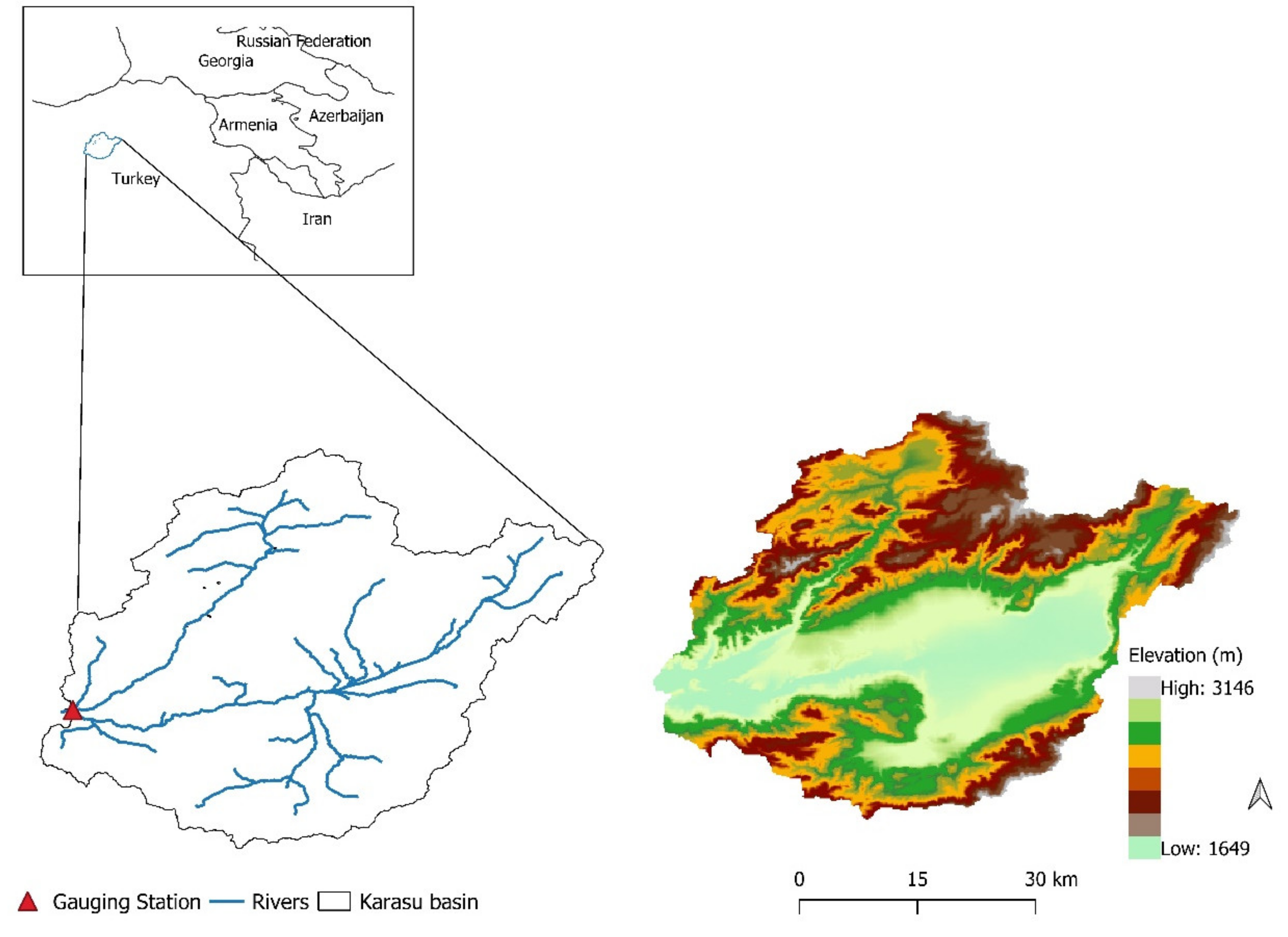
The study area is the Karasu basin located at the Euphrates River’s headwaters in Turkey (Figure 1). The basin is mostly dominated by pasture, grass and bare land. The total area is about 2886 km2. This area is hugely mountainous with an elevation range of 1125–3500 m and mean basin slope of 20%. Karasu Basin boundaries are within the longitudes 38°58′ E to 41°39′ E and latitudes 39°23′ N to 40°25′ N. Studies showed that 60–70% of the total annual runoff volume comes during snowmelt season. The annual mean precipitation of the basin fluctuates from 400 to 450 mm/year [31]. Streamflow data for the Karasu basin are collected by General Directorate of Turkish State Hydraulic Works (DSI) at the Karasu Aşağı Kağdarıç gauging station (#6695500-GRDC ID or #2154-Local ID) [32]. The basin downstream is characterized by huge dams that make accurate runoff estimation crucial to efficient water resources allocation for flood control, hydropower generation, irrigation, and water supply [33].
2.2. Model Description
The mHM is a fully distributed hydrologic model based on numerical approximations of hydrologic processes such as canopy interception, snow accumulation and melting, soil moisture dynamics, infiltration and surface runoff, evaporation, subsurface storage and discharge generation, deep percolation and base flow, and discharge attenuation and flood routing [34]. The model discretization in this setup is based on grid cells of 0.0625° spatial resolution, with each grid generating runoff that is routed using adaptive timestep, constant celerity routing method. The mHM utilizes a Multiscale Parameter Regionalization technique to account for sub-grid variability of catchment morphology [35,36,37] which enables the swapping between different scales while calculating all fluxes and routing streamflow on a preferred model scale. The model contains 62 global parameters that can be adjusted during the calibration process and pedo-transfer functions for soil parameterization [35]. Samaniego et al. [38] can be consulted for explicit description of model formulation and parameter description. The mHM was preferred as the interest model due to its three unique features (1) multiscale parameter regionalization technique, which links basin’s physical characteristics to parameter value via pedo-transfer functions (2) ability to process multiple LULC data (3) use of leaf area index (LAI) data not only for calculating interception loss but also for correcting PET.
2.3. Data Preparation
The basic data for setting up the mHM can be classified into meteorological data, morphological data, land cover data and gauging station data. The essential meteorological variables are the precipitation and average air temperature at hourly to daily temporal resolution. However, based on a strategy of estimating potential evapotranspiration, additional data like net radiation, wind speed, the absolute vapor pressure of air, potential evapotranspiration, maximum and minimum air temperature. The morphological variables are the digital elevation model, soil maps with textural properties, geological maps containing specific yield, permeability and aquifer thickness. For this study, the E-OBS dataset was utilized with the precipitation, average air temperature data and potential evapotranspiration obtained from Rakovec et al. [39] with a resolution of 0.25° and daily time steps, input directly into the model, hence no need for its estimation in the model (Table 1). All morphological data are provided at a resolution of 0.001953° and the meteorological data at 0.25°. The model is run at a daily time-step with and outputs are internally resampled to a spatial resolution of 0.0625° by the model.
2.4. Land Cover Data
The Coordination of Information on the Environment (CORINE), MODIS and GLOBCOVER land cover data were used. The Coordination of Information on the Environment (CORINE) Land Cover (CLC) is the first land cover map in Europe based on photographic interpretation of Landsat-5, Landsat-7 ETM, SPOT-4/5, IRS P6 LIS III, Sentinel-2 and Landsat-8 satellite images for the years 1990, 2000, 2006, 2012 and 2018. The geometric accuracy of all the images are ≤25 m except Landsat-5 and Sentinel-2 images, with accuracy ≤50 m and ≤10 m respectively, producing the CLC 1990, CLC 2000, CLC 2006, CLC 2012 and CLC 2018 products respectively. The spatial resolutions of the products are 100 m and 250 m, [40] with the land cover inventoried into 44 classes [41]. The main advantage of the CORINE Land Cover (CLC) inventory is its frequent update by European countries, although the level of detail of the source data is a limitation [41]. This limitation suggests that the CLC inventory is a useful resource for land cover change studies on the regional scale. The MODIS Land Cover collection is a global land cover data set designed to support research related to current, seasonal to the decadal status of global land properties, with 17 land cover classes at a 500 m spatial resolution and yearly temporal coverage with a 71.6% overall accuracy [40]. The GLOBCOVER dataset is a global project initiated by European Space Agency (ESA) in conjunction with the Joint Research Centre (JRC), the European Environment Agency (EEA), the Global Observation of Forests Cover and Land Dynamic (GOFC-GOLD), Food and Agriculture Organization (FAO), the United Nations Environment Program (UNEP) and the International Geosphere-Biosphere Program (IGBP) [42]. The project entailed the generation of world land cover map using 300 m Medium Resolution Imaging Spectrometer (MERIS) instrument aboard ENVISAT [43]. The mHM identifies only three land cover classification. This classification includes forest (coniferous and deciduous), impervious (urban and built-up areas, water bodies, and consolidated soils), and pervious (grasslands, croplands, and bare soil) [34]. Hence, the land cover data were reclassified to suit the data requirements.
2.5. Sensitivity Analysis
Hydrologic models are associated with uncertainties, which have always prompted researchers better to understand the hydrologic process and better representation in models. These models are associated with some level of complexities that vary among models to represent necessary variables correctly. Sensitivity Analysis (SA) is a method employed by modelers to deal with these complexities during calibration by analyzing the contribution of each model parameter to the uncertainty in model prediction. The basis for SA is an effect called the “Sparsity of Factors” principle. This principle, which originates from the field of Statistical Design of Experiments, states that when a process is influenced by several variables, its behavior is likely driven by a small subset of these variables [44]. These subsets of variables characterize sources of uncertainties in model prediction and upon which research towards model performance improvement should be focused [45]. SA can summarily be applied for assessment of model similarities [46], obtaining regions of sensitivity [47], factor and model reduction [48] and uncertainty apportionment [49]. In this study, we used PEST Tool [9] to assess most important parameters based on Jacobian matrix to include in the model calibration.
2.6. Model Calibration and Validation
In this study, four different cases (Table 2) based on input data were created to achieve the set objectives. These cases contain different configurations and representations of hydrologic processes. The Case 1 (C1) model was configured using one-year GLOBCOVER land cover data and no correction of PET data using LAI information in the region. The PET data was only subjected to correction with the aspect of the grid cells. The Case 2 (C2) model was also configured with the same land cover data but with LAI correction. This strategy allows the PET data to be corrected based on the LAI data supplied to the model. The Case 3 (C3) model was configured with multiple land cover data from a different database. It contained 1990 and 2000 CORINE land cover data and consecutive MODIS land cover data from 2001 to 2008 for the calibration period. The PET data, in this case, is also subjected to only the aspect correction and ignores the LAI correction. The Case 4 (C4) model contains the same land cover configuration as C3; however, the PET data were subjected to LAI correction. The model was calibrated with the discharge data from the gauging station from 1990 to 2006 while 2007 to 2010 was used for the validation.
2.7. Dynamically Dimensioned Search Algorithm (DDS)
The DDS was developed to obtain best global solutions within a model evaluation limit based on heuristic global search algorithm [50]. The DDS algorithm begins its search globally and becomes localized as the iteration numbers approaches the limit of function evaluations. This is achieved by decreasing the number of dimensions in the neighborhood dynamically and probabilistically, and further distribute the reducing probability equally to each decision variable [51]. The need to modify parameters simultaneously during calibration to preserve the current gain in calibration result was the motivation behind the algorithm. The critical feature of DDS was triggered by the poor result associated with manual calibration of watersheds especially with progress in the calibration process. It becomes necessary to calibrate one or few parameters simultaneously as calibration result improves in order to prevent loss of previously gained result [50].
2.8. Model Performance
The Nash-Sutcliffe efficiency (NSE) was used to evaluate the integrity of the model simulations for each scenario. This objective function quantifies the accuracy of prediction by comparing the differences between predicted and observed discharge values. NSE is a scaled metric that compares the expected variable with the observed variable’s mean as the naïve forecast. An efficiency of zero, indicates that using the observed data as forecast would give the same error as the predicted data, a negative efficiency means that the mean of the observed data is a better predictor than the model prediction [52]. The inverse (NSEinv) and logarithm (NSEln) of this metric was also adopted to capture the flow dynamics. Pushpalatha et al. [53] reported that NSEln and NSEinv are useful metrics for the evaluation of low flows, although the latter shows no sensitivity to high flows unlike the NSEln, which shows little sensitivity, and NSE, which is highly sensitivity to high flows. The Kling-Gupta Efficiency (KGE) was also adopted to evaluate the annual flows [54]. KGE consists of three components targeted at addressing the flaws observed in NSE. This evaluation criterion is based on NSE decomposition into the linear correlation between observed and simulated flows, the flow variability term and biased term [55]. The optimum value is 1 and unlike NSE, KGE does not have an inherent benchmark against which flows are compared and the value to be compared is subjective to the modeler [56]. Other evaluation criteria used are PBIAS and Mean Absolute Error (MAE), which measured the simulated values’ average tendency to be larger or smaller than their observed ones and the absolute difference between observed and simulated flows respectively. The optimum value of MAE is 0 and low magnitude values indicates accurate model prediction. Positive values of PBIAS indicate some overestimation of predicted data while negative values indicates model underestimation of predicted values.
Stagl and Hattermann [57] suggested the use of some hydrological indices for the evaluation of model simulation. For this study, the long-term annual average discharge, flow in dry season, high flows (Q10), low flows (Q90), flow in wet season and base flow were selected as indices to evaluate the modeled cases. The wet season was taken from May to October while the rest of the months were considered as dry season. The base flow was estimated as 30% of the average daily flow and the performance was evaluated using the procedure alighted in Chirachawala et al. [58], which is the absolute difference between each calibrated case and its corresponding value in the observed case.
3. Results
3.1. Land Use Land Cover Variations
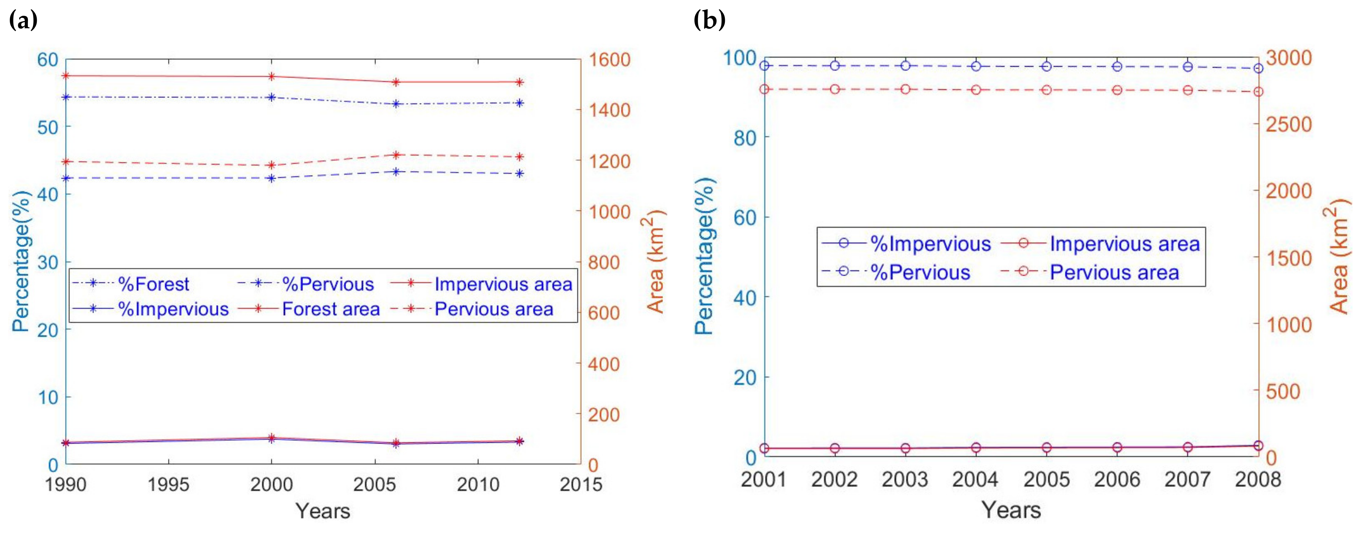
LULC maps in physically distributed hydrological models are essential inputs for efficient modeling of spatial variations in hydrologic fluxes, excess rainfall and infiltration in particular. This study adopted the CORINE and MODIS LULC dataset and the changes in the land cover characteristics shown in Figure 2 using the mHM recognized land cover classes.
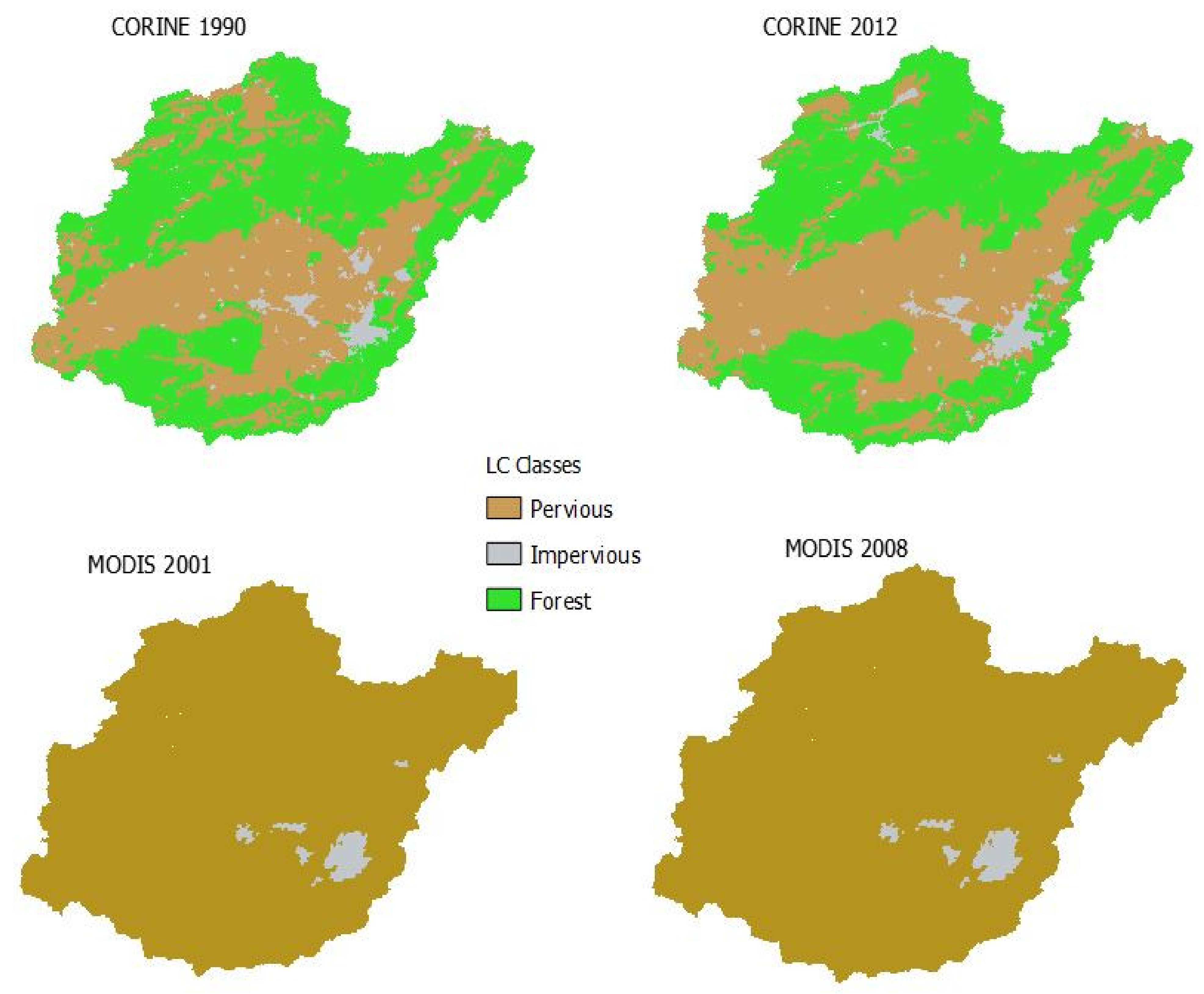
The variation in land cover classes between the upper and lowest land cover map adopted is also shown in Figure A1. Using the conventional CORINE land cover nomenclature to characterize the land cover in the basin as shown in Table A1, the most dominant land cover obtained in the study period is the natural grasslands, which increased from 718.63 km2 in 1990 to 929.63 km2 in 2012, although a slight decline was noticed in 2000 before the increase in subsequent years. A significant increase in the area covered by water bodies was also observed. In 1990, 0.04% of the watershed, which is 1.1 km2, is covered by water. This increased to 11.17 km2 in 2000 and varied annually until it reached 9.42 km2 in 2012. Road networks in the basin occupied the least land cover in the studied maps covering 0.013% of the total basin area in 1990 and expanded to 0.054% in 2012. Artificial surfaces like buildings, roads, industry and land cover comprising of urban fabrics increased by 7.35% between 1990 and 2012. This may be responsible for the decrease in the agricultural areas from 1194.53 km2 to 1139km2, indicating about 4.7% decline. In the same vein, forest areas declined by 6.3% between 1990 and 2012. Glacier and perpetual snow in the watershed were observed to cover more area in 2012. In 1990, the snow area was around 434.62 km2 and steadily increased annually in the observed maps to 473.98 km2 in 2012. However, the hydrologic model of interest was designed to recognize three land cover classifications; forest, impervious and pervious. MODIS has no separate forest class in the study domain after reclassification but more frequent (yearly) observations than CORINE, hence these two land cover products complement each other.
3.2. Sensitivity Analysis
Sensitivity analysis in this study was used to identify model parameters sensitive to discharge prediction in the basin using the Parameter Estimation and Uncertainty Analysis (PEST) tool [9]. PEST performs all calibration tasks, including sensitivity and uncertainty analysis, upon the user needs. The tool allowed the identification of the sensitive parameters to discharge prediction in the model set up and these were normalized using the maximum sensitivity value. Of the 62 global parameters in the model, 20 parameters were selected as most sensitive as shown in Table A2 and they were afterwards used to calibrate the hydrologic model.
The mHM parameters are divided into groups based on the processes they influence. The soil moisture parameters were observed to be very sensitive to the model output, although this sensitivity varies among the parameters. Eleven of these parameters out of about twenty soil moisture parameters were sensitive in the setup. This actually depends on the method used for modeling soil water movement, the Feddes equation was used in this study. The sensitivity of PET parameters differs with choice of PET estimation method. For this study, PET correction using LAI and aspect maps were eventually adopted. The PET parameters related to correction using LAI parameters were found to be sensitive. The process of interflow was also found to be sensitive to streamflow predictions in the model set up. This was shown in the sensitivity analysis characterized with 3 out of the 5 interflow parameters showing huge sensitivity. Lastly, the percolation process, through the recharge coefficient parameter was found to be sensitive to the streamflow dynamics in the study area. These sensitive parameters were selected to calibrate the model to obtain optimum parameter values with 3000 iterations.
3.3. Model Calibration
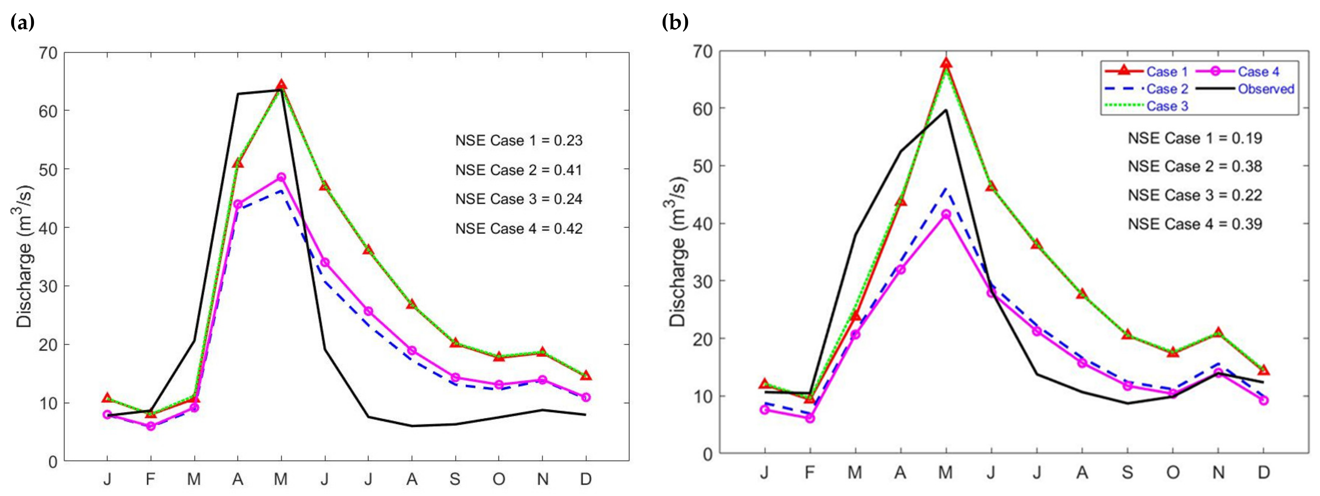
All four cases were calibrated with the sensitive parameters obtained from the sensitivity analysis. These cases are used to consider the simultaneous effect of PET correction technique and multiple LULC maps. The estimated NSE value ranges between 0.226 and 0.422, with the highest in Case 4 and the lowest at Case 1 respectively. PBIAS and MAE value for Case 1 and Case 3 were the highest, indicating a better performance, with Case 2 and Case 4 the better cases. KGE values for the modeled cases during calibration ranges between 0.419 and 0.544 for the calibration, with Case 4 having the highest KGE value indicating the best performance with this metric. NSEln and NSEinv were adopted to filter out the high flow sensitivity of conventional NSE during estimation. The range of NSEln was −0.36 and 0.05 while that of NSEinv was −0.65 and −0.61. Considering the individual effect of PET correction method on the model performance, Case 1 and Case 2 were configured with the same input data but different PET correction method. Case 3 and Case 4 were also configured with the same input data but different PET correction method. In this vein, the NSE value of Case 2 revealed higher value than that of Case 1 while that of Case 4 also revealed a higher NSE value than that of Case 3. To isolate the effect of multiple land cover data on the model, Case 1 and Case 3 were configured with the same input dataset but different land cover configuration. Case 2 and Case 4 were also configured with the same input data but different land cover configuration. In this comparison, Case 3 and Case 4 proved better with higher NSE values. KGE values for these cases also follows the same pattern with the Case 4 having the best performance among the cases as shown in Table 3.
3.4. Model Validation
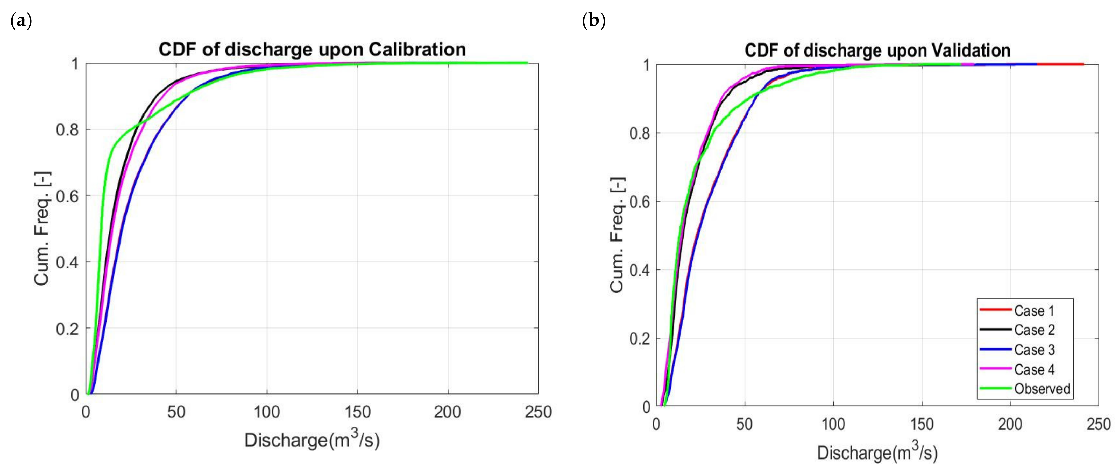
For the validation phase, the NSE value obtained were slightly lower than the calibration phase ranging from 0.19 and 0.39, with the Case 4 also showing the best performance. The NSEln metric revealed its highest value as Case 2 and the lowest with Case 3, recording efficiency of 0.26 and −0.07 respectively. KGE also recorded its highest value in Case 2 and lowest in Case 4. However, Case 4 performed better under MAE, with the lowest value among the observed Cases as shown in Table 3. The hydrograph of the observed and simulated average monthly discharges for all the cases is shown in Figure 3 and the cumulative distribution frequency of daily discharge data is shown in Figure A2 should be noted that all cases underestimated the frequency of the discharge until it reached about 1000 m3/s, when Case 2 and Case 4 overestimated the frequency, as did the other cases when the discharge accumulated to about 1400 m3/s.
3.5. Hydrological Indices
The annual discharge, wet season flows, dry season flows and base flow of the modeled cases were used to evaluate the model’s performance by comparing them with the observed data from the gauging station, as shown in Table 4. For annual discharge, wet season flows, low flows and dry season flows, Case 2 performed better than the others, although Case 4 also performs optimally. For annual discharge, the percentage difference of Case 2 is 2.89% while that of the worst performance is Case 3, with a percentage difference of 44.37%. The dry season flow performance showed a different trend, with Case 3 performing better than the other cases, with a percentage difference of 1.62% against the lowest performing case, which was Case 2 with a difference of 22.7%. Finally, for the high flows, case 1 has the lowest percentage difference of 1.48%, indicating the best scenario for this flow type.
To show the effect of misclassification of land cover on discharge, monthly discharge in the basin was predicted by providing the model with CORINE 2006 and MODIS 2006 sequentially. The CORINE land cover product characterized with forest, pervious and impervious land cover predicted higher discharges between May and October, while the MODIS land cover product with just pervious and impervious classes simulated higher discharges for the rest of the months.
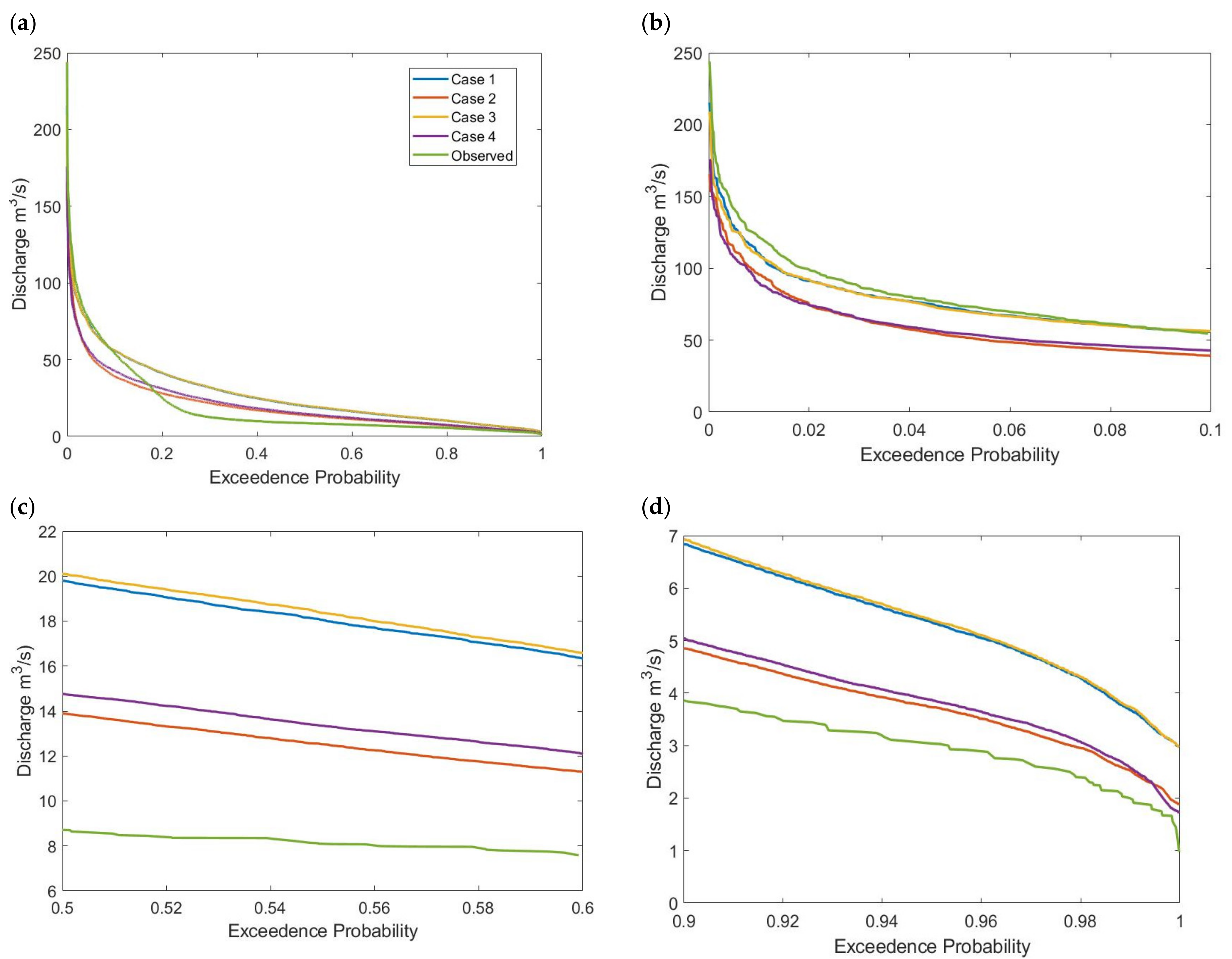
The flow duration curve (FDC) is an important tool in hydrology to summarize streamflow time series [59]. This study below applies FDC to observe the exceedance probabilities of flows and further divides the flow into high flow, low flow and median flow. Flows less or equal to 10% exceedance are characterized as high flows, flows between 50 and 60% exceedance probabilities are median flows and those beyond 90% exceedance probabilities are low flows.
Flow duration curves as shown in Figure 4 describes the flow characteristics in the basin and the variation in the different modeled cases. For the high flows as shown in Figure 4b, case 1 and case 3 seems to capture the flows better and closer to the observed flow. However, for the median and low flows, cases 2 and 4, configured with LAI data provided optimum simulation that captures the flow.
4. Discussion
The need to estimate the impacts of climate and land use change on discharge regime has made hydrologic models popular worldwide, especially with their ability to predict flows at gauges and ungauged catchments. However, these predictions are subjected to uncertainty due to model bias, input data errors, and errors in model parameter values [60]. The goal of hydrologic modelers is to reduce uncertainties associated with the model outputs upon which decision about hydrologic fluxes are based. There have been numerous studies focusing on different ways to improve model performance by exploring various input data characteristics that affects the predictions in conceptual and physically distributed models [17,18,19,61,62,63]. Models like mHM are spatially distributed since they consist of equations involving one or more space coordinates, which are used for simulation of spatial variation in hydrological variables within a catchment as well as simple outflows and bulk storage volumes. Such models make considerable demands in terms of computational time and data requirements and are costly to develop and operate [6]. The results presented in this study provide the spatial model’s response to varying characteristics of the input data based on the objective under study. Recall that the scenarios labeled as Case 1 to Case 4 and their varying input characteristics. Case 1 and Case 2 were configured with single LULC data, with LAI influence on the Case 2 only. The same applies to Case 3 and Case 4 but with multiple land cover classes, which makes it possible to observe LAI’s effect on the model performance. LAI is a key biophysical vegetation property for interception that describes biome-specific canopy structure and an essential variable in evaluating the interrelation of the components of the water-soil-plant-atmosphere system, which influences environmental studies [64]. The vegetation of an area due to its LAI is a significant component of land surface models that influence evapotranspiration simulation and, consequently, affects base flow, recharge, infiltration excess, saturation excess, subsurface storm flow and catchment wetness [25]. As hypothesized, the cases LAI data performed better than their counterparts during calibration and validation process. The implication is that predictions are more accurate when leaf area index is included in the model for correction on evapotranspiration. Precise evaluation of evapotranspiration is a vital aspect of water balance estimation. About 60% of terrestrial precipitation returns to the atmosphere by plant transpiration (40%), or through direct soil evaporation (20%) [65]. The correct simulations of LAI seasonal dynamics and stomatal aperture in an eco-hydrological model are prerequisite of good simulation of canopy radiation exchanges and transpiration fluxes which are important components of the accurate water balance estimation [66].
Furthermore, the impact of single and multiple land cover data was observed. The result associated better model performance with the cases with multiple land cover data. This corroborates Jin et al., [1], where the use of multiple land-use datasets improved model performance although with some complexities in simulation complexity due to greater number of LULC patches. LULC maps are essential input of physically distributed models since they spatially delineate the basin’s different morphological characteristics that decide water’s fate on the earth’s surface. A detailed characterization of land cover is essential for urban areas, as coarse spatial description might result in biased estimates by hiding urban heterogeneous evapotranspiration [67]. Petrucci & Bonhomme [68] also found a similar result to our study where increasing geographical information clearly improves model performances with the land use classification providing the highest benefit. Finally, considering the combined effect of both morphological characteristics, the case with multiple land cover data and LAI to correct evapotranspiration performed better than the other cases and the case with single land cover data, without LAI correction performed worse. It is noteworthy that the discharge data were used in the model’s calibration, which leaves the possibility of variation in model performance if different calibration method or data was used. The data-intensive nature of physically distributed models often leads to over-parameterization while effectively representing each hydrologic process that constitutes such a model. This opens up another phase of research in hydrologic modeling to solve over-parameterization and identify strategies to improve model performance without overwhelming the model with information.
FDC provides an indepth response of the flow to varying configurations of the model set up. While the total FDC gives a general response of the basin to the stream flow timeseries, focusing on the response of specific flow type sheds essential information for various aspects of water resources management, such as high flows for dam construction and low flows for irrigation mangement [69].
5. Conclusions
Hydrologic modeling remains an important decision support tool for efficiently allocating water resources and solving global water security issues, especially with the climate’s non-stationarity and changing land use. The model outputs are characterized with some degree of uncertainty by underestimating or overestimating the simulated values. The best models are thus characterized with reduced uncertainties, and different methods are being adopted to achieve this. This study explored the impact of LULC maps and LAI on the performance of a fully distributed hydrologic model. Various model cases were set up to evaluate the independent effects of LAI and LULC map on model performance. The result showed that using LAI for accurate estimation of evapotranspiration values adopted for the simulation of hydrologic processes increased the model performance when the model was calibrated using discharge data. In addition to this, providing mHM with multiple LULC datasets has better performance than those with single LUCL data. This study reiterated the observation of Jin et al. [1] about the impact of multiple land cover datasets on model performance. We further suggest using optimum land cover dataset when available to enable the model to capture recent and relevant LULC patches that will be utilized in the simulation of the hydrologic processes. Especially in rapidly developing landscapes, this will be necessary to capture the basin dynamics. Furthermore, in the absence of multiple or yearly LULC maps, other strategies that will reduce model uncertainty like using LAI data for accurate estimation of evapotranspiration can be adopted.
Author Contributions
I.O.B. and M.C.D. provided the morphological and meteorological data, M.C.D. performed the sensitivity analysis, and I.O.B. performed the calibration and validation of the model. I.O.B. and M.C.D. performed the visualization of the result. The concept of the study and the draft manuscript were written and reviewed by I.O.B., M.C.D. and A.N. All authors have read and agreed to the published version of the manuscript.
Funding
The first author is supported by the European Union through the Erasmus Mundus Scholarship program. The second author (MCD) is supported by the SPACE project fund from the Villum Foundation (http://villumfonden.dk/) through their Young Investigator Programme (grant VKR023443) the National Center for High Performance Computing of Turkey (UHeM) under grant number 1007292019.
Institutional Review Board Statement
Not applicable.
Informed Consent Statement
Not applicable.
Data Availability Statement
All data sources are listed in Table 1. Karasu basin model set-up data were kindly provided by Oldrich Rakovec from UFZ in Leipzig, Germany. Discharge data is publicly available at the repository of State Hydraulic Work (DSİ) https://www.dsi.gov.tr/Sayfa/Detay/744, and daily data from the gauging station was compiled and then provided by Dr. Muhammet Yılmaz. Due to data license restrictions, the observed geographical, hydrological and meteorological data cannot be redistributed from the authors but can be obtained from Rakovec et al. [39], respective organizations and/or UFZ in Leipzig, Germany, upon request. The model calibration results can be retrieved from the corresponding author upon request. The source code of the mHM is publicly available at https://doi.org/10.5281/zenodo.4575390.
Acknowledgments
We thank Ali Arda Şorman and İsmail Bilal Peker for their fruitful discussions on the data and study area. We also thank the three anonymous reviewers and editors for their constructive comments.
Conflicts of Interest
The authors declare no conflict of interest.
Appendix A
Figure A1.
Selected CORINE and MODIS land cover maps of the study area for CORINE 1990, CORINE 2012, MODIS 2001 and MODIS 2008.
Figure A1.
Selected CORINE and MODIS land cover maps of the study area for CORINE 1990, CORINE 2012, MODIS 2001 and MODIS 2008.

Figure A2.
Cumulative distribution function of observed and simulated daily discharge (a) calibration (b) validation.
Figure A2.
Cumulative distribution function of observed and simulated daily discharge (a) calibration (b) validation.


Table A1.
Detailed Land cover statistics in Karasu Basin for the selected years using CORINE land cover data.
Table A1.
Detailed Land cover statistics in Karasu Basin for the selected years using CORINE land cover data.
| CORINE Land Cover Classes | Years | |||||||
|---|---|---|---|---|---|---|---|---|
| 1990 | 2000 | 2006 | 2012 | |||||
| %Land Cover | Area km2 | %Land Cover | Area km2 | %Land Cover | Area km2 | %Land Cover | Area km2 | |
| Continuous urban fabric | 0.05 | 1.33 | 0.04 | 1.23 | 0.07 | 1.92 | 0.57 | 16.13 |
| Discontinuous urban fabric | 1.35 | 38.15 | 1.48 | 41.77 | 1.12 | 31.49 | 0.67 | 18.98 |
| Industrial or commercial units | 0.41 | 11.62 | 0.48 | 13.45 | 0.58 | 16.22 | 0.57 | 15.99 |
| Road and rail networks | 0.01 | 0.37 | 0.05 | 1.49 | 0.02 | 0.64 | 0.05 | 1.52 |
| Airports | 0.31 | 8.77 | 0.31 | 8.83 | 0.31 | 8.83 | 0.32 | 9.02 |
| Mineral extraction sites | 0.08 | 2.14 | 0.11 | 3.20 | 0.14 | 3.93 | 0.17 | 4.85 |
| Construction sites | - | - | 0.02 | 0.60 | 0.02 | 0.57 | 0.05 | 1.44 |
| Green urban areas | 0.02 | 0.48 | 0.02 | 0.67 | 0.02 | 0.68 | 0.01 | 0.25 |
| Sport and leisure facilities | 0.22 | 6.15 | 0.21 | 5.83 | 0.18 | 5.14 | 0.21 | 5.89 |
| Non-irrigated arable land | 18.07 | 509.51 | 18.08 | 509.72 | 5.36 | 151.21 | 5.30 | 149.53 |
| Permanently irrigated land | 8.29 | 233.87 | 8.23 | 232.04 | 17.45 | 492.00 | 17.42 | 491.15 |
| Pastures | 2.25 | 63.45 | 2.15 | 60.74 | 4.64 | 130.93 | 4.43 | 125.00 |
| Complex cultivation patterns | 4.19 | 118.15 | 3.97 | 111.93 | 6.25 | 176.34 | 6.26 | 176.63 |
| Land principally occupied by agriculture with significant areas of natural vegetation | 9.56 | 269.55 | 9.39 | 264.73 | 9.60 | 270.74 | 9.61 | 270.95 |
| Broad-leaved forest | 0.78 | 21.88 | 0.82 | 23.07 | 0.51 | 14.37 | 0.48 | 13.45 |
| Coniferous forest | 0.12 | 3.44 | 0.14 | 4.02 | 0.14 | 3.87 | 0.14 | 4.06 |
| Mixed forest | 0.74 | 20.87 | 0.75 | 21.25 | 0.27 | 7.51 | 0.24 | 6.82 |
| Natural grasslands | 25.49 | 718.63 | 25.38 | 715.67 | 31.65 | 892.50 | 32.97 | 929.63 |
| Transitional woodland-shrub | 11.32 | 319.20 | 11.29 | 318.43 | 3.55 | 100.22 | 2.19 | 61.87 |
| Beaches dunes sands | 0.12 | 3.38 | 0.10 | 2.66 | 0.23 | 6.60 | 0.23 | 6.46 |
| Bare rocks | 0.37 | 10.46 | 0.37 | 10.30 | 0.42 | 11.96 | 0.43 | 12.15 |
| Glaciers and perpetual snow | 15.41 | 434.62 | 15.41 | 434.52 | 16.71 | 471.20 | 16.81 | 473.98 |
| Inland marshes | 0.62 | 17.40 | 0.63 | 17.64 | 0.17 | 4.64 | 0.35 | 9.81 |
| Water bodies | 0.04 | 1.10 | 0.40 | 11.17 | 0.41 | 11.45 | 0.33 | 9.42 |
Table A2.
Normalized sensitivity parameters.
| Parameters | Range | Normalized Sensitivity |
|---|---|---|
| Rotfrcoffore | 0.9–0.999 | 1.00000 |
| pet_aforest | 0.2999–1.3 | 0.48665 |
| pet_apervi | 0.2999–1.3 | 0.14471 |
| Ptflowconst | 0.6462–0.9506 | 0.14227 |
| Infshapef | 1.0–4.0 | 0.09453 |
| ptflowdb | −0.3726–0.1870999 | 0.07084 |
| pet_aimpervi | 0.29999–1.3000 | 0.01222 |
| ptflowclay | 0.0001–0.00289 | 0.01091 |
| rotfrcofimp | 0.9–0.9499 | 0.00945 |
| ptfkssand | 0.006–0.02599 | 0.00339 |
| ptfksconst | −1.2–0.28499 | 0.00841 |
| ptfhigconst | 0.5358–1.1232 | 0.00793 |
| rotfrcofclay | 0.9–0.999 | 0.00339 |
| expslwintflw | 0.05–0.3 | 0.00095 |
| rechargcoef | 0–50.0 | 0.00044 |
| intrecesslp | 0–10.0 | 0.00040 |
| slwintreceks | 1.0–30.0 | 0.00040 |
| pet_bb | 0–1.5 | 0.00039 |
| pet_cc | −2.0–0 | 0.00031 |
| Rotfrcofsand | 0.001–0.09 | 0.00002 |
References
- Jin, X.; Jin, Y.; Yuan, D.; Mao, X. Effects of land-use data resolution on hydrologic modelling, a case study in the upper reach of the Heihe River, Northwest China. Ecol. Modell. 2019, 404, 61–68. [Google Scholar] [CrossRef]
- Moges, E.; Demissie, Y.; Larsen, L.; Yassin, F. Review: Sources of hydrological model uncertainties and advances in their analysis. Water 2021, 13, 28. [Google Scholar] [CrossRef]
- Gan, T.Y.; Biftu, G.F. Effects of model complexity and structure, parameter interactions and data on watershed modeling. In Calibration of Watershed Models; American Geophysical Union: Washington, DC, USA, 2004; pp. 317–329. ISBN 087590355X. [Google Scholar]
- Bulygina, N.; Gupta, H. Estimating the uncertain mathematical structure of a water balance model via Bayesian data assimilation. Water Resour. Res. 2009, 45. [Google Scholar] [CrossRef]
- Son, K.; Sivapalan, M. Improving model structure and reducing parameter uncertainty in conceptual water balance models through the use of auxiliary data. Water Resour. Res. 2007, 43. [Google Scholar] [CrossRef]
- Lohani, A.K. Rainfall-Runoff Analysis and Modelling; National Institute of Hydrology: Roorkee, India, 2018. [Google Scholar]
- Beven, K.; Binley, A. The future of distributed models: Model calibration and uncertainty prediction. Hydrol. Process. 1992, 6, 279–298. [Google Scholar] [CrossRef]
- Vrugt, J.A. Markov chain Monte Carlo simulation using the DREAM software package: Theory, concepts, and MATLAB implementation. Environ. Model. Softw. 2016, 75, 273–316. [Google Scholar] [CrossRef] [Green Version]
- Doherty, J. PEST: Model-Independent Parameter Estimation, User Manual, 5th ed.; Watermark Numerical Computing: Brisbane, Australia, 2010. [Google Scholar]
- Camargos, C.; Julich, S.; Houska, T.; Bach, M.; Breuer, L. Effects of input data content on the uncertainty of simulatingwater resources. Water 2018, 10, 621. [Google Scholar] [CrossRef] [Green Version]
- Devia, G.K.; Ganasri, B.P.; Dwarakish, G.S. A Review on Hydrological Models. Aquat. Procedia 2015, 4, 1001–1007. [Google Scholar] [CrossRef]
- Younghun, J.; Venkatesh, M. Uncertainty Quantification in Flood Inundation Mapping Using Generalized Likelihood Uncertainty Estimate and Sensitivity Analysis. J. Hydrol. Eng. 2012, 17, 507–520. [Google Scholar] [CrossRef]
- Muleta, M.K.; McMillan, J.; Amenu, G.G.; Burian, S.J. Bayesian Approach for Uncertainty Analysis of an Urban Storm Water Model and Its Application to a Heavily Urbanized Watershed. J. Hydrol. Eng. 2013, 18, 1360–1371. [Google Scholar] [CrossRef]
- Rampinelli, C.G.; Knack, I.; Smith, T. Flood Mapping Uncertainty from a Restoration Perspective: A Practical Case Study. Water 2020, 12, 1948. [Google Scholar] [CrossRef]
- Bouslihim, Y.; Rochdi, A.; El Amrani Paaza, N.; Liuzzo, L. Understanding the effects of soil data quality on SWAT model performance and hydrological processes in Tamedroust watershed (Morocco). J. Afr. Earth Sci. 2019, 160, 103616. [Google Scholar] [CrossRef]
- Ficchì, A.; Perrin, C.; Andréassian, V. Impact of temporal resolution of inputs on hydrological model performance: An analysis based on 2400 flood events. J. Hydrol. 2016, 538, 454–470. [Google Scholar] [CrossRef]
- Li, C.Z.; Wang, H.; Liu, J.; Yan, D.H.; Yu, F.L.; Zhang, L. Effect of calibration data series length on performance and optimal parameters of hydrological model. Water Sci. Eng. 2010, 3, 378–393. [Google Scholar] [CrossRef]
- Ilampooranan, I.; Schnoor, J.L.; Basu, N.B. Crops as sensors: Using crop yield data to increase the robustness of hydrologic and biogeochemical models. J. Hydrol. 2020, 125599. [Google Scholar] [CrossRef]
- Orth, R.; Staudinger, M.; Seneviratne, S.I.; Seibert, J.; Zappa, M. Does model performance improve with complexity? A case study with three hydrological models. J. Hydrol. 2015, 523, 147–159. [Google Scholar] [CrossRef] [Green Version]
- Srivastava, A.; Kumari, N.; Maza, M. Hydrological Response to Agricultural Land Use Heterogeneity Using Variable Infiltration Capacity Model. Water Resour. Manag. 2020, 34, 3779–3794. [Google Scholar] [CrossRef]
- Aghsaei, H.; Mobarghaee Dinan, N.; Moridi, A.; Asadolahi, Z.; Delavar, M.; Fohrer, N.; Wagner, P.D. Effects of dynamic land use/land cover change on water resources and sediment yield in the Anzali wetland catchment, Gilan, Iran. Sci. Total Environ. 2020, 712, 136449. [Google Scholar] [CrossRef] [PubMed]
- Setyorini, A.; Khare, D.; Pingale, S.M. Simulating the impact of land use/land cover change and climate variability on watershed hydrology in the Upper Brantas basin, Indonesia. Appl. Geomat. 2017, 9, 191–204. [Google Scholar] [CrossRef]
- Boongaling, C.G.K.; Faustino-Eslava, D.V.; Lansigan, F.P. Modeling land use change impacts on hydrology and the use of landscape metrics as tools for watershed management: The case of an ungauged catchment in the Philippines. Land Use Policy 2018, 72, 116–128. [Google Scholar] [CrossRef]
- Das, P.; Behera, M.D.; Patidar, N.; Sahoo, B.; Tripathi, P.; Behera, P.R.; Srivastava, S.K.; Roy, P.S.; Thakur, P.; Agrawal, S.P.; et al. Impact of LULC change on the runoff, base flow and evapotranspiration dynamics in eastern Indian river basins during 1985–2005 using variable infiltration capacity approach. J. Earth Syst. Sci. 2018, 127, 1–19. [Google Scholar] [CrossRef] [Green Version]
- Tesemma, Z.K.; Wei, Y.; Peel, M.C.; Western, A.W. The effect of year-to-year variability of leaf area index on Variable Infiltration Capacity model performance and simulation of runoff. Adv. Water Resour. 2015, 83, 310–322. [Google Scholar] [CrossRef] [Green Version]
- Chen, Y.; Niu, J.; Kang, S.; Zhang, X. Effects of irrigation on water and energy balances in the Heihe River basin using VIC model under different irrigation scenarios. Sci. Total Environ. 2018, 645, 1183–1193. [Google Scholar] [CrossRef]
- Al-Safi, H.I.J.; Sarukkalige, P.R. The application of conceptual modelling to assess the impacts of future climate change on the hydrological response of the Harvey River catchment. J. Hydro-Environ. Res. 2020, 28, 22–33. [Google Scholar] [CrossRef]
- Bisht, D.S.; Mohite, A.R.; Jena, P.P.; Khatun, A.; Chatterjee, C.; Raghuwanshi, N.S.; Singh, R.; Sahoo, B. Impact of climate change on streamflow regime of a large Indian river basin using a novel monthly hybrid bias correction technique and a conceptual modeling framework. J. Hydrol. 2020, 590, 125448. [Google Scholar] [CrossRef]
- Singh Jasrotia, A.; Baru, D.; Kour, R.; Ahmad, S.; Kour, K. Hydrological modeling to simulate stream flow under changing climate conditions in Jhelum catchment, western Himalaya. J. Hydrol. 2021, 593, 125887. [Google Scholar] [CrossRef]
- Paul, P.K.; Kumari, N.; Panigrahi, N.; Mishra, A.; Singh, R. Implementation of cell-to-cell routing scheme in a large scale conceptual hydrological model. Environ. Model. Softw. 2018, 101, 23–33. [Google Scholar] [CrossRef]
- Uysal, G.; Şorman, A.A.; Şensoy, A. Streamflow Forecasting Using Different Neural Network Models with Satellite Data for a Snow Dominated Region in Turkey. Procedia Eng. 2016, 154, 1185–1192. [Google Scholar] [CrossRef] [Green Version]
- Ertas, C.; Akkol, B.; Coskun, C.; Uysal, G.; Sorman, A.A.; Sensoy, A. Evaluation of Probabilistic Streamflow Forecasts Based on EPS for a Mountainous Basin in Turkey. Procedia Eng. 2016, 154, 490–497. [Google Scholar] [CrossRef] [Green Version]
- Tekeli, A.E.; Akyürek, Z.; Şorman, A.A.; Şensoy, A.; Şorman, A.Ü. Using MODIS snow cover maps in modeling snowmelt runoff process in the eastern part of Turkey. Remote Sens. Environ. 2005, 97, 216–230. [Google Scholar] [CrossRef]
- Dembélé, M.; Hrachowitz, M.; Savenije, H.H.G.; Mariéthoz, G.; Schaefli, B. Improving the Predictive Skill of a Distributed Hydrological Model by Calibration on Spatial Patterns with Multiple Satellite Data Sets. Water Resour. Res. 2020, 56, 1–26. [Google Scholar] [CrossRef]
- Demirel, M.C.; Koch, J.; Mendiguren, G.; Stisen, S. Spatial pattern oriented multicriteria sensitivity analysis of a distributed hydrologic model. Water 2018, 1188. [Google Scholar] [CrossRef] [Green Version]
- Dembélé, M.; Ceperley, N.; Zwart, S.J.; Salvadore, E.; Mariethoz, G.; Schaefli, B. Potential of satellite and reanalysis evaporation datasets for hydrological modelling under various model calibration strategies. Adv. Water Resour. 2020, 143. [Google Scholar] [CrossRef]
- Höllering, S.; Wienhöfer, J.; Ihringer, J.; Samaniego, L.; Zehe, E. Regional analysis of parameter sensitivity for simulation of streamflow and hydrological fingerprints. Hydrol. Earth Syst. Sci. 2018, 22, 203–220. [Google Scholar] [CrossRef] [Green Version]
- Samaniego, L.; Kumar, R.; Attinger, S. Multiscale parameter regionalization of a grid-based hydrologic model at the mesoscale. Water Resour. Res. 2010, 46. [Google Scholar] [CrossRef] [Green Version]
- Rakovec, O.; Kumar, R.; Mai, J.; Cuntz, M.; Thober, S.; Zink, M.; Attinger, S.; Schäfer, D.; Schrön, M.; Samaniego, L. Multiscale and Multivariate Evaluation of Water Fluxes and States over European River Basins. J. Hydrometeorol. 2016, 17, 287–307. [Google Scholar] [CrossRef]
- Grekousis, G.; Mountrakis, G.; Kavouras, M. An overview of 21 global and 43 regional land-cover mapping products. Int. J. Remote Sens. 2015, 36, 5309–5335. [Google Scholar] [CrossRef]
- Cieślak, I.; Biłozor, A.; Źróbek-Sokolnik, A.; Zagroba, M. The use of geographic databases for analyzing changes in land cover—A case study of the region of warmia and mazury in Poland. ISPRS Int. J. Geo-Inf. 2020, 9, 358. [Google Scholar] [CrossRef]
- An, Y.; Zhao, W.; Zhang, Y. Accuracy assessments of the GLOBCOVER dataset using global statistical inventories and FLUXNET site data. Acta Ecol. Sin. 2012, 32, 314–320. [Google Scholar] [CrossRef]
- Tchuenté, A.T.K.; Roujean, J.L.; de Jong, S.M. Comparison and relative quality assessment of the GLC2000, GLOBCOVER, MODIS and ECOCLIMAP land cover data sets at the African continental scale. Int. J. Appl. Earth Obs. Geoinf. 2011, 13, 207–219. [Google Scholar] [CrossRef]
- Box, G.E.P.; Meyer, R.D. An Analysis for Unreplicated Fractional Factorials. Technometrics 1986, 28, 11–18. [Google Scholar] [CrossRef]
- Razavi, S.; Sheikholeslami, R.; Gupta, H.V.; Haghnegahdar, A. VARS-TOOL: A toolbox for comprehensive, efficient, and robust sensitivity and uncertainty analysis. Environ. Model. Softw. 2019, 112, 95–107. [Google Scholar] [CrossRef]
- Clark, M.P.; Kavetski, D.; Fenicia, F. Pursuing the method of multiple working hypotheses for hydrological modeling. Water Resour. Res. 2011, 47, 1–16. [Google Scholar] [CrossRef] [Green Version]
- Rakovec, O.; Hill, M.C.; Clark, M.P.; Weerts, A.H.; Teuling, A.J.; Uijlenhoet, R. Distributed evaluation of local sensitivity analysis (DELSA), with application to hydrologic models. Water Resour. Res. 2014, 50, 409–426. [Google Scholar] [CrossRef] [Green Version]
- Nossent, J.; Elsen, P.; Bauwens, W. Sobol’ sensitivity analysis of a complex environmental model. Environ. Model. Softw. 2011, 26, 1515–1525. [Google Scholar] [CrossRef]
- Chu-Agor, M.L.; Muñoz-Carpena, R.; Kiker, G.; Emanuelsson, A.; Linkov, I. Exploring vulnerability of coastal habitats to sea level rise through global sensitivity and uncertainty analyses. Environ. Model. Softw. 2011, 26, 593–604. [Google Scholar] [CrossRef]
- Tolson, B.A.; Shoemaker, C.A. Dynamically dimensioned search algorithm for computationally efficient watershed model calibration. Water Resour. Res. 2007, 43, 1–16. [Google Scholar] [CrossRef]
- Chu, J.; Peng, Y.; Ding, W.; Li, Y. A Heuristic dynamically dimensioned search with sensitivity information (HDDS-S) and application to river basin management. Water 2015, 7, 2214. [Google Scholar] [CrossRef] [Green Version]
- Jackson, E.K.; Roberts, W.; Nelsen, B.; Williams, G.P.; Nelson, E.J.; Ames, D.P. Introductory overview: Error metrics for hydrologic modelling—A review of common practices and an open source library to facilitate use and adoption. Environ. Model. Softw. 2019, 119, 32–48. [Google Scholar] [CrossRef]
- Pushpalatha, R.; Perrin, C.; Le Moine, N.; Andréassian, V. A review of efficiency criteria suitable for evaluating low-flow simulations. J. Hydrol. 2012, 420–421, 171–182. [Google Scholar] [CrossRef]
- Kling, H.; Gupta, H. On the development of regionalization relationships for lumped watershed models: The impact of ignoring sub-basin scale variability. J. Hydrol. 2009, 373, 337–351. [Google Scholar] [CrossRef]
- Gupta, H.V.; Kling, H.; Yilmaz, K.K.; Martinez, G.F. Decomposition of the mean squared error and NSE performance criteria: Implications for improving hydrological modelling. J. Hydrol. 2009, 377, 80–91. [Google Scholar] [CrossRef] [Green Version]
- Knoben, W.J.M.; Freer, J.E.; Woods, R.A. Technical note: Inherent benchmark or not? Comparing Nash-Sutcliffe and Kling-Gupta efficiency scores. Hydrol. Earth Syst. Sci. Discuss. 2019, 1–7. [Google Scholar] [CrossRef] [Green Version]
- Stagl, J.C.; Hattermann, F.F. Impacts of Climate Change on Riverine Ecosystems: Alterations of Ecologically Relevant Flow Dynamics in the Danube River and Its Major Tributaries. Water 2016, 8, 566. [Google Scholar] [CrossRef] [Green Version]
- Chirachawala, C.; Shrestha, S.; Babel, M.S.; Virdis, S.G.P.; Wichakul, S. Evaluation of global land use/land cover products for hydrologic simulation in the Upper Yom River Basin, Thailand. Sci. Total Environ. 2020, 708, 135148. [Google Scholar] [CrossRef]
- Brown, A.E.; Western, A.W.; McMahon, T.A.; Zhang, L. Impact of forest cover changes on annual streamflow and flow duration curves. J. Hydrol. 2013, 483, 39–50. [Google Scholar] [CrossRef]
- Deckers, D. Predicting Discharge at Ungauged Catchments: Parameter Estimation through the Method of Regionalisation; University of Twente: Enschede, The Netherlands, 2006. [Google Scholar]
- Sahraei, S.; Asadzadeh, M.; Unduche, F. Signature-based multi-modelling and multi-objective calibration of hydrologic models: Application in flood forecasting for Canadian Prairies. J. Hydrol. 2020, 588, 125095. [Google Scholar] [CrossRef]
- Bai, P.; Liu, X.; Zhang, Y.; Liu, C. Incorporating vegetation dynamics noticeably improved performance of hydrological model under vegetation greening. Sci. Total Environ. 2018, 643, 610–622. [Google Scholar] [CrossRef]
- Gao, J.; Sheshukov, A.Y.; Yen, H.; Kastens, J.H.; Peterson, D.L. Impacts of incorporating dominant crop rotation patterns as primary land use change on hydrologic model performance. Agric. Ecosyst. Environ. 2017, 247, 33–42. [Google Scholar] [CrossRef]
- Hardwick, S.R.; Toumi, R.; Pfeifer, M.; Turner, E.C.; Nilus, R.; Ewers, R.M. The relationship between leaf area index and microclimate in tropical forest and oil palm plantation: Forest disturbance drives changes in microclimate. Agric. For. Meteorol. 2015, 201, 187–195. [Google Scholar] [CrossRef] [Green Version]
- Di, N.; Wang, Y.; Clothier, B.; Liu, Y.; Jia, L.; Xi, B.; Shi, H. Modeling soil evaporation and the response of the crop coefficient to leaf area index in mature Populus tomentosa plantations growing under different soil water availabilities. Agric. For. Meteorol. 2019, 264, 125–137. [Google Scholar] [CrossRef]
- Fatichi, S.; Vivoni, E.R.; Ogden, F.L.; Ivanov, V.Y.; Mirus, B.; Gochis, D.; Downer, C.W.; Camporese, M.; Davison, J.H.; Ebel, B.; et al. An overview of current applications, challenges, and future trends in distributed process-based models in hydrology. J. Hydrol. 2016, 537, 45–60. [Google Scholar] [CrossRef] [Green Version]
- Elga, S.; Jan, B.; Okke, B. Hydrological modelling of urbanized catchments: A review and future directions. J. Hydrol. 2015, 529, 62–81. [Google Scholar] [CrossRef]
- Petrucci, G.; Bonhomme, C. The dilemma of spatial representation for urban hydrology semi-distributed modelling: Trade-offs among complexity, calibration and geographical data. J. Hydrol. 2014, 517, 997–1007. [Google Scholar] [CrossRef]
- Sapač, K.; Medved, A.; Rusjan, S.; Bezak, N. Investigation of low- and high-flow characteristics of karst catchments under climate change. Water 2019, 11, 925. [Google Scholar] [CrossRef] [Green Version]
Figure 1.
The location of the Karasu Basin and the elevation.

Figure 2.
Land cover evolution in Karasu basin (a) CORINE (b) MODIS.

Figure 3.
Observed and simulated average monthly discharge of designed 4 cases. (a) Calibration (b) Validation.
Figure 3.
Observed and simulated average monthly discharge of designed 4 cases. (a) Calibration (b) Validation.

Figure 4.
Flow Duration Curve for (a) total flows (b) high flows (0–10%) (c) median flows (50–60%) (d) low flows (90–100%).
Figure 4.
Flow Duration Curve for (a) total flows (b) high flows (0–10%) (c) median flows (50–60%) (d) low flows (90–100%).

Table 1.
Overview of input datasets.
| Variable | Description | Spatial Resolution | Source |
|---|---|---|---|
| Q (daily) | Streamflow | Point | Karasu Aşağı Kağdariç station (#6695500-GRDC ID or #2154-Local ID) |
| P (daily) | Precipitation | 0.25° | E-OBS 20.0e |
| ETref (daily) | Reference evapotranspiration | 0.25° | E-OBS 20.0e |
| Tavg (daily) | Average air temperature | 0.25° | E-OBS 20.0e, MODIS |
| Land cover | Pervious, impervious and forest | 0.001953° | CORINE, MODIS, GlobcoverV2 |
| DEM data | Slope, aspect, flow accumulation and direction | 0.001953° | SRTM |
| Geology class | Two main geological formations | 0.001953° | EUROPEAN SOIL DATABASE |
| Soil class | Soil texture data | 0.001953° | HARMONIZED WORLD SOIL DATABASE |
Table 2.
Description of the model cases.
| Ase | Land Cover Input | PET Correction with LAI |
|---|---|---|
| 1 | 1 year Globcover dataset | No |
| 2 | 1 year Globcover dataset | Yes |
| 3 | MODIS and CORINE datasets | No |
| 4 | MODIS and CORINE datasets | Yes |
Table 3.
Performance assessment of the different cases.
| NSE (-) | NSEln | NSEinv | PBIAS (%) | KGE | MAE (m3/s) | |||||||
|---|---|---|---|---|---|---|---|---|---|---|---|---|
| Cal | Val | Cal | Val | Cal | Val | Cal | Val | Cal | Val | Cal | Val | |
| Case 1 | 0.23 | 0.19 | −0.36 | −0.08 | −0.63 | −0.38 | 43.5 | 29.2 | 0.42 | 0.51 | 15.9 | 15.1 |
| Case 2 | 0.41 | 0.38 | 0.05 | 0.26 | −0.61 | −0.48 | 2.8 | −10.8 | 0.54 | 0.52 | 12 | 10.8 |
| Case 3 | 0.24 | 0.22 | −0.36 | −0.07 | −0.63 | −0.36 | 44.2 | 30.2 | 0.42 | 0.51 | 15.9 | 15 |
| Case 4 | 0.42 | 0.39 | −0.02 | 0.23 | −0.65 | −0.89 | 8.8 | −16.7 | 0.54 | 0.48 | 12.3 | 10.6 |
Table 4.
Performance of mHM in simulating hydrological indices.
| Hydrological Indices | Case | Difference (%) |
|---|---|---|
| Annual Discharge | Case 1 | 43.63 |
| Case 2 | 2.89 * | |
| Case 3 | 44.37 | |
| Case 4 | 8.96 | |
| High flows (Q10) | Case 1 | 1.48 * |
| Case 2 | 15.21 | |
| Case 3 | 1.93 | |
| Case 4 | 11.53 | |
| Low flows (Q90) | Case 1 | 2.96 |
| Case 2 | 0.97 * | |
| Case 3 | 3.05 | |
| Case 4 | 1.16 | |
| Wet flows | Case 1 | 91.97 |
| Case 2 | 29.50 * | |
| Case 3 | 92.18 | |
| Case 4 | 40.21 | |
| Dry flows | Case 1 | 2.88 |
| Case 2 | 22.7 | |
| Case 3 | 1.62 * | |
| Case 4 | 21.1 | |
| Base flow | Case 1 | 43.45 |
| Case 2 | 2.78 * | |
| Case 3 | 44.19 | |
| Case 4 | 8.83 |
* Bold indicates lowest (best) cases.
Publisher’s Note: MDPI stays neutral with regard to jurisdictional claims in published maps and institutional affiliations. |
© 2021 by the authors. Licensee MDPI, Basel, Switzerland. This article is an open access article distributed under the terms and conditions of the Creative Commons Attribution (CC BY) license (https://creativecommons.org/licenses/by/4.0/).
Share and Cite
MDPI and ACS Style
Busari, I.O.; Demirel, M.C.; Newton, A. Effect of Using Multi-Year Land Use Land Cover and Monthly LAI Inputs on the Calibration of a Distributed Hydrologic Model. Water 2021, 13, 1538. https://doi.org/10.3390/w13111538
AMA Style
Busari IO, Demirel MC, Newton A. Effect of Using Multi-Year Land Use Land Cover and Monthly LAI Inputs on the Calibration of a Distributed Hydrologic Model. Water. 2021; 13(11):1538. https://doi.org/10.3390/w13111538
Chicago/Turabian StyleBusari, Ibrahim Olayode, Mehmet Cüneyd Demirel, and Alice Newton. 2021. "Effect of Using Multi-Year Land Use Land Cover and Monthly LAI Inputs on the Calibration of a Distributed Hydrologic Model" Water 13, no. 11: 1538. https://doi.org/10.3390/w13111538
Note that from the first issue of 2016, this journal uses article numbers instead of page numbers. See further details here.