Erosion Transportation Processes as Influenced by Gully Land Consolidation Projects in Highly Managed Small Watersheds in the Loess Hilly–Gully Region, China

Abstract

The Loess Hilly–Gully region (LHGR) is the most serious soil erosion area in the world. For the small watershed with high management in this area, the scientific problem that has been paid attention to in recent years is the impact of the land consolidation project on the erosion environment in the gully region. In this study, the 3D simulation method of vegetation, eroded sediment and pollutant transport was innovated based on the principles of erosion sediment dynamics and similarity theory, and the impacts of GLCP were analyzed on the erosion environment at different scales. The verification results show that the design method and the scale conversion relationship (geometric scale: ${\mathsf{\lambda }}_{\mathrm{l}}$ = 100) were reasonable and could simulate the transport process on the complex underlying surface of a small watershed. Compared with untreated watersheds, a significant change was the current flood peak lagging behind the sediment peak. There were two important critical values of GLCP impact on the erosion environment. The erosion transport in HMSW had no change when the proportion was less than 0.85%, and increased obviously when it was greater than 3.3%. The above results have important theoretical and practical significance for watershed simulation and land-use management in HMSW.

1. Introduction

Worldwide, the Loess Plateau is well known for its intense soil erosion and has received more attention from both the government and academic spheres [1,2,3]. To cope with this, the Chinese central government implemented the Grain for Green project in the 1990s and achieved a significant reduction [4,5,6]. However, what followed was a severe shortage of high-quality land [7,8]. Therefore, to solidify the achievements of the Grain for Green project and address the problem of the shortage of high-quality land resources, a series of experiments and demonstrations have been carried out since 2010, mainly including the transformation of abandoned silt dams and the cutting of conditional trench slopes to fill the trenches and prepare the land [9,10,11,12,13]. On the basis of the successful experience gained, a large-scale project, “Gully Land Consolidation (GLC)” has begun in the Loess Hilly and Gully Region (LHGR), especially in the small watershed with high management and obvious weakening of erosion. Its impact on runoff and sediment changes and environment has attracted wide attention from domestic and oversea scholars [14,15,16].

The impact of land-use pattern on the erosion environment has always been valued by researchers around the world [17,18]. Some researchers believed that land consolidation in the gully raised the erosion base level and helped to reduce sediment erosion [19,20,21]. However, some scholars believed that the LHGR was deeply covered with loess, and was highly collapsible. Thus, it was necessary to prevent the disasters caused by collapsibility [22,23] in order to reduce the ecological impact of GLCP on peak discharge, sediment production, NH₄-N, NO₃-N and CO₂ emissions with an enhanced soil organic carbon (SOC) relative to the undisturbed gully [24]. However, more than 2000 ha farmland were damaged by dam breaks and landslide under the extreme rainstorm in Yanan in 2013 [13,25], which was one of the controversies regarding the impact of land consolidation on the erosional ecological environment [26,27].

On all these counts, the previous studies of [28,29,30,31,32,33,34,35] stated both the positive and negative impact of land consolidation on the erosion environment and they did not pay attention to whether the scale and proportion of land consolidation led to changes in the ecological environment. The proportion of land consolidation refers to the ratio of the area of land consolidation to the total area of the basin. Would there be a critical value for the consolidation ratio? When it was less than the critical value, the impact of the land improvement project on the environment was not significant, and when it is greater than this value, it might have a greater impact. However, there were not many studies on this area.

In this study, a physical scale watershed model was selected to carry out the experiments. The objectives of this study were to: (1) investigate the pollutant similarity rules; (2) characterize the effects of management measures on water and sediment processes; and (3) determine the critical land consolidation proportion.

2. Materials and Methods

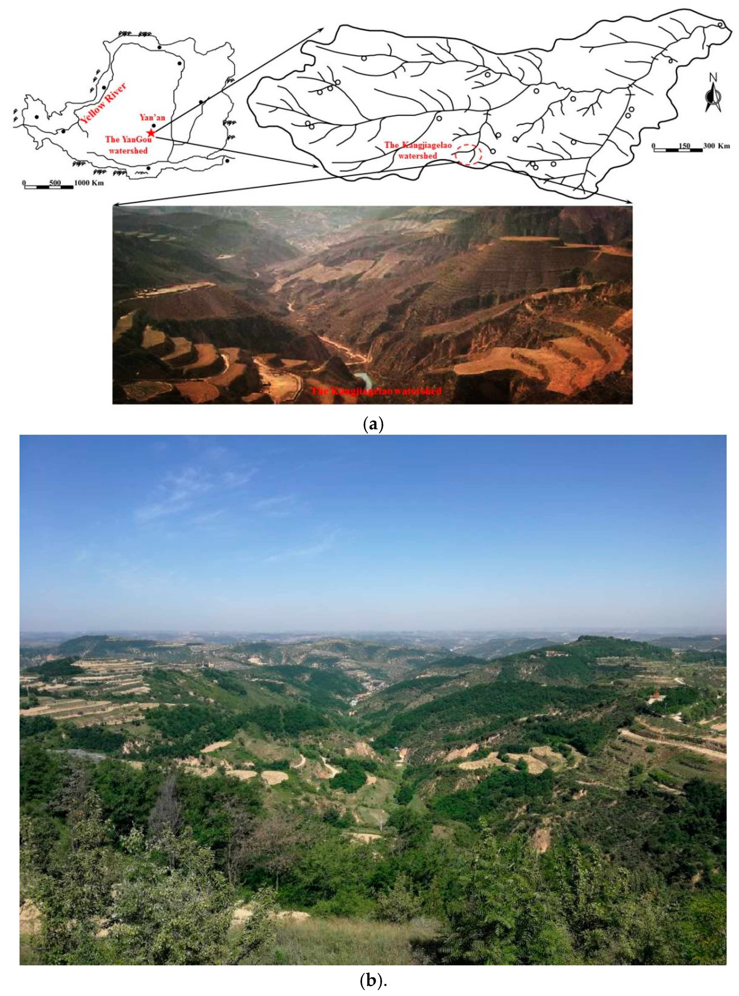
2.1. Study Area

The Yangou watershed (36°21′–36°22′ N, 109°20′–109°35′ E) is located in the southern suburbs of Yan’an city in the middle of the LHGR (as shown in Figure 1), with an area of about 48 km² and an annual rainfall of 575 mm. The Kangjiagelao small watershed is located in the Yangou watershed, covering an area of 0.35 km² and a height of 189.7 m, having a silt dam with a length of 11 m and a width of 5 m at the outlet of the gully. The terraced farmlands and terraced orchards in the watershed account for 15–20% of the total watershed area, and the remaining area contains arbores, shrubs, and herbaceous vegetation. The watershed vegetation coverage is more than 90%. It is an ideal prototype area for the study of GLCP practices based on “Grain for Green” management.

Gao et al. [36,37] provided a largely complete set of design methods and techniques for simulating rainfall, runoff, and sediment transport in the small Kangjiagelao watershed, which were based on the hydrodynamic principles of rainfall, runoff, sediment transport, infiltration, and similarity theory. The model was normal and the geometric scale was 100. The verification results demonstrated that the rainfall, runoff collection, and sediment generation and transport were in line with the actual observations for similar geometries, rainfall, eroded sediment generation, transport processes, and surface bed deformation. These results were used to generate recommendations regarding methods for controlling soil erosion, optimizing design plans, and seeking efficient use of water and soil resources [36,37].

Figure 2 shows the sediment curves of the prototype and model. The model D₅₀ parameter was set to 0.027 mm, which is near the value of 0.028 mm used in the prototype. The soil selection of the model met the requirements.

Table 1. The land-use patterns and vegetation coverage in the Kangjiagelao watershed.

Land-Use Pattern	Area (km2)	Vegetation Height (m)	Vegetation Coverage (%)
Terraced farmland	0.028	0.2–0.4	80
Terraced orchard	0.042	2–2.5	75
Arbor	0.140	8–12	95
Shrub	0.088	1.5–2	95
Grassland	0.035	0.45–0.6	92
Water cellar	0.018	0	0

presents the land-use status acquired by a survey completed in 2018, which reported the land-use mode, occupied area, vegetation type, vegetation height, and coverage degree. The average vegetation coverage of the prototype small watershed in Yangou reached 0.9. A vegetation coverage scale of 1 was obtained via geometric similarity. The small watershed model was restored according to the current vegetation coverage of the small watershed after management. The model built according to the two situations of no vegetation restoration and high-level vegetation restoration is shown in Figure 3.

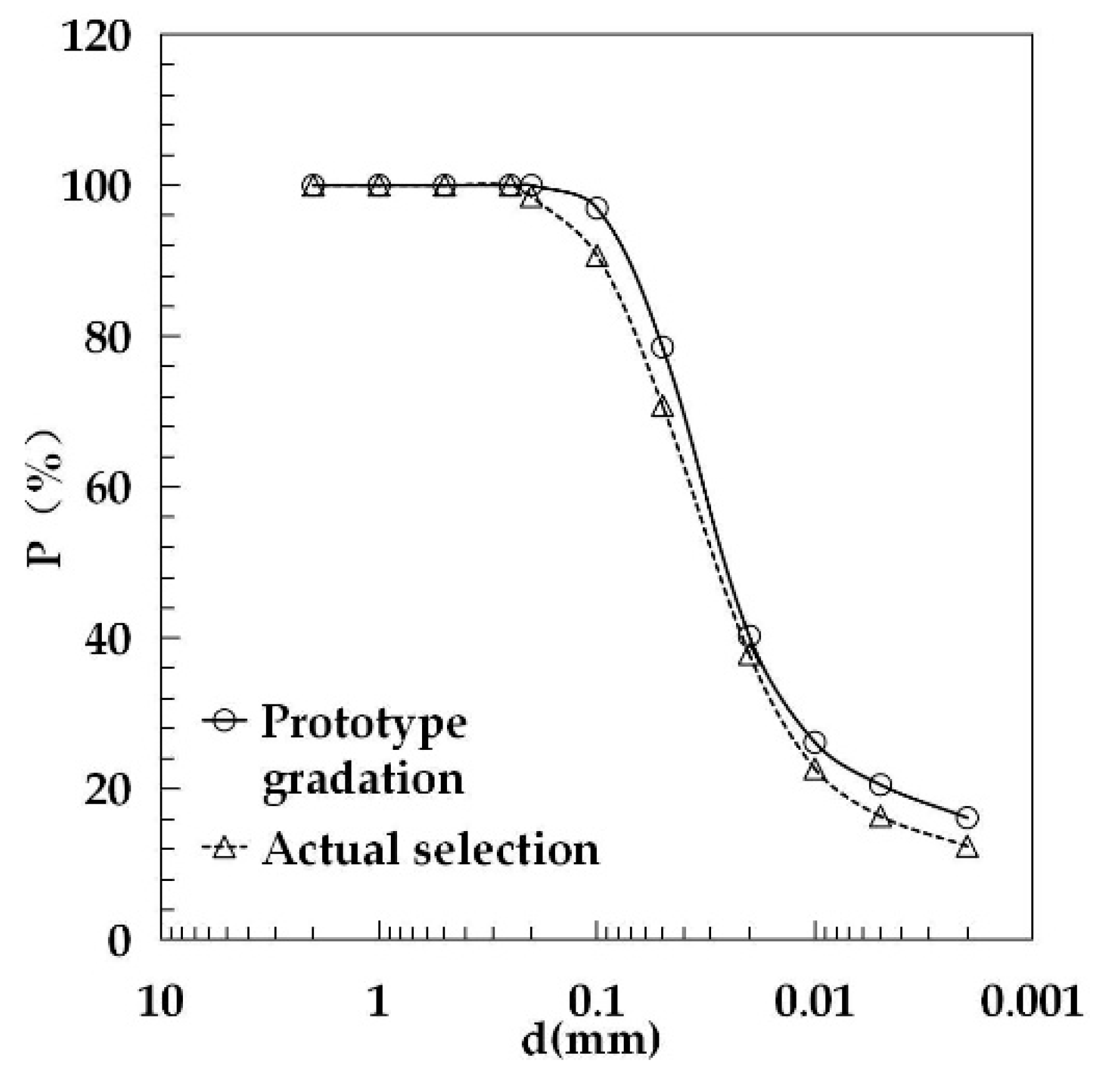
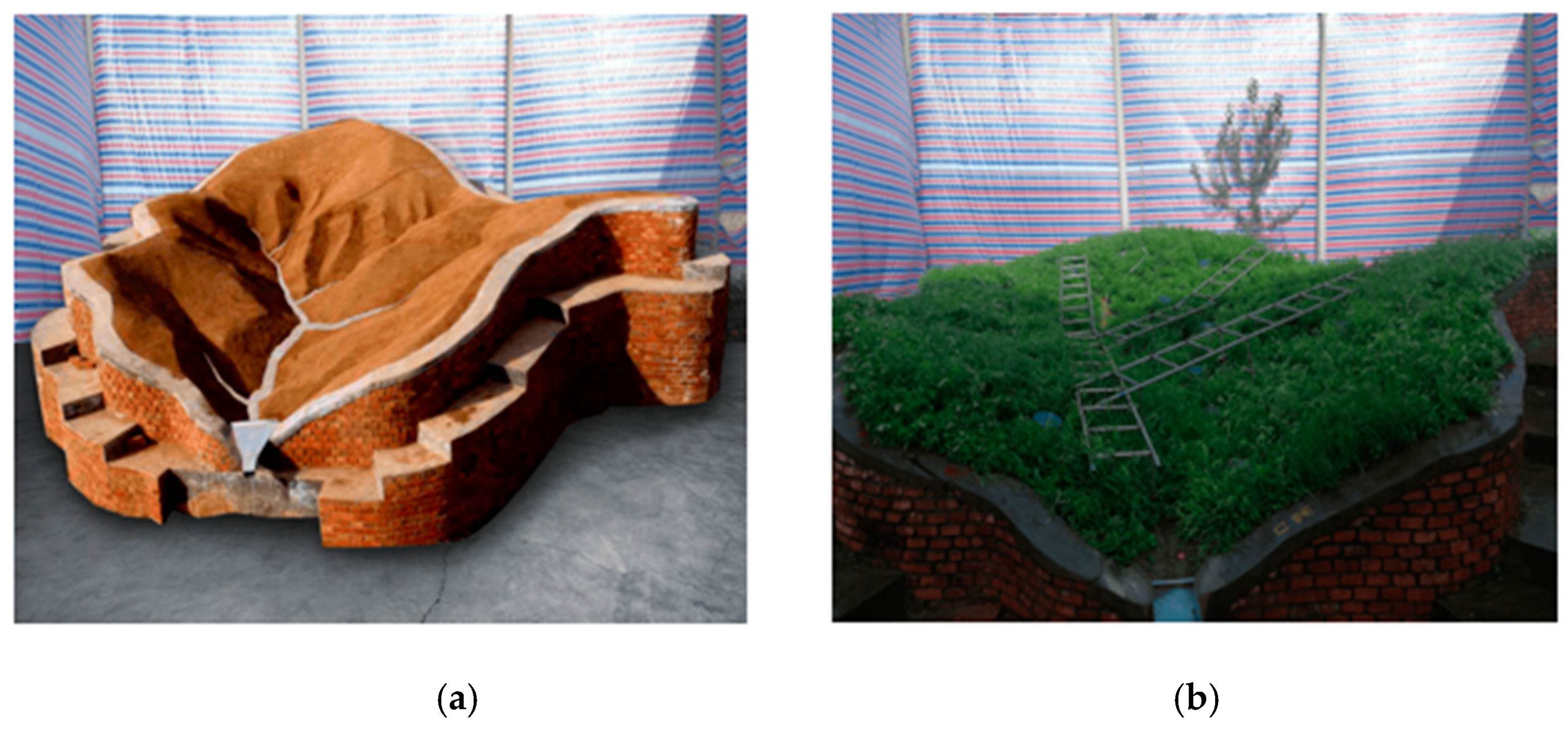
2.2. Model Principle and Scale Design

Since the 3D simulation of the watershed needs to simulate the rainfall, runoff and erosion transport on the slope and gully, the physical model used in this experiment meets the following basic principles:

2.2.1. Rainfall Runoff on Slope

On the slope surface, assuming that the direction of the water flow is the x-axis and the slope length is L, then the one-dimensional unstable flow slope Saint-Venant equations that control the movement of the slope surface flow are:

$$\frac{\partial (Vy)}{\partial x}+\frac{\partial y}{\partial t} = i(x,t)-i_0(x,t) = r(x,t)$$

(1)

$$J_0-J_F = \frac{\partial y}{\partial x}+\frac{1}{g}\frac{\partial V}{\partial t}+\frac{V}{g}\frac{\partial V}{\partial x}+\frac{V}{gy}\left[i(x,t)-f(x,t)\right]$$

(2)

where y is the flow depth of the slope, V is the flow velocity of the slope, i(x,t) is rain intensity as a function of x and t, f(x,t) is the infiltration strength as a function of x and t, r is the net rain intensity as a function of x and t, r(x,t) = i(x,t) − f(x,t) adopt the international standard unit m·s⁻¹, J₀ is the slope grade, J_F is the friction slope, and g is the acceleration of gravity.

2.2.2. Gully Water Movement

As the slope of the simulated small watershed is steep, and the current is turbulent, the runoff is mostly caused by short-duration torrential rains. Therefore, turbulence has been fully developed during the confluence of slopes and channels. Therefore, the time-averaged differential equation describing the three-dimensional turbulence of the incompressible fluid can be used to describe the water movement.

Continuous equation:

$$\frac{\partial \overline{u}}{\partial \chi }+\frac{\partial \overline{\upsilon }}{\partial y}+\frac{\partial \overline{\omega }}{\partial z} = 0$$

(3)

Equation of motion:

$$\begin{gathered} \frac{\partial \overline{u}}{\partial t}+(\overline{u}\frac{\partial \overline{u}}{\partial x}+\overline{\upsilon }\frac{\partial \overline{u}}{\partial y}+\overline{\omega }\frac{\partial \overline{u}}{\partial z}) \\ = F_x-\frac{1}{\rho }\frac{\partial \overline{p}}{\partial x}+\left[\frac{\partial }{\partial x}\left(v\frac{\partial \overline{u}}{\partial x}\right)+\frac{\partial }{\partial y}\left(v\frac{\partial \overline{u}}{\partial y}\right)+\frac{\partial }{\partial z}\left(v\frac{\partial \overline{u}}{\partial z}\right)\right]-\left(\frac{\partial }{\partial x}\overline{u^{12}}+\frac{\partial }{\partial u}\overline{u^{\prime }{\upsilon }^{\prime }}+\frac{\partial }{\partial z}\overline{u^{\prime }{\omega }^{\prime }}\right) \end{gathered}$$

(4)

$$\begin{gathered} \frac{\partial \overline{\upsilon }}{\partial t}+(\overline{u}\frac{\partial \overline{u}}{\partial x}+\overline{\upsilon }\frac{\partial \overline{\upsilon }}{\partial y}+\overline{\omega }\frac{\partial \overline{\upsilon }}{\partial z}) \\ = F_y-\frac{1}{\rho }\frac{\partial \overline{p}}{\partial y}+\left[\frac{\partial }{\partial x}\left(v\frac{\partial \overline{\upsilon }}{\partial x}\right)+\frac{\partial }{\partial y}\left(v\frac{\partial \overline{\upsilon }}{\partial y}\right)+\frac{\partial }{\partial z}\left(v\frac{\partial \overline{\upsilon }}{\partial z}\right)\right]-\left(\frac{\partial }{\partial x}\overline{u^{\prime }{\upsilon }^{\prime }}+\frac{\partial }{\partial y}\overline{{\upsilon }^{\prime 2}}+\frac{\partial }{\partial z}\overline{{\upsilon }^{\prime }{\omega }^{\prime }}\right) \end{gathered}$$

(5)

$$\begin{gathered} \frac{\partial \overline{w}}{\partial t}+(\overline{u}\frac{\partial \overline{w}}{\partial x}+\overline{\upsilon }\frac{\partial \overline{w}}{\partial y}+\overline{\omega }\frac{\partial \overline{w}}{\partial z}) \\ {F}_z-\frac{1}{\rho }\frac{\partial \overline{p}}{\partial z}+\left[\frac{\partial }{\partial x}\left(v\frac{\partial \overline{w}}{\partial x}\right)+\frac{\partial }{\partial y}\left(v\frac{\partial \overline{w}}{\partial y}\right)+\frac{\partial }{\partial z}\left(v\frac{\partial \overline{w}}{\partial z}\right)\right]-\left(\frac{\partial }{\partial x}\overline{u^{\prime }{w}^{\prime }}+\frac{\partial }{\partial y}\overline{{\upsilon }^{\prime }{w}^{\prime }}+\frac{\partial }{\partial z}\overline{w^{\prime 2}}\right) \end{gathered}$$

(6)

where $\overline{u}$, $\overline{\upsilon }$, $\overline{\omega }$ are the time-average flow velocity along the x, y, and z axes, $u$, $\upsilon$, $\omega$ are the pulsating flow velocity along the x, y, and z axes, F_x, F_y, F_z are the mass forces per unit mass along the x, y, and z axes, when the mass force is limited to gravity, its value is equal to the components of the acceleration of gravity along the x, y, and z axes, when the x-axis is consistent with the direction of water flow, $F_x = g\sin \alpha$, $F_y = -g\cos \alpha$, $F_z = g\sin \beta = g{J}_z$, where $\alpha$ and $\beta$ are the inclination angles of the water flow along the x and z directions, $J_x$, $J_z$ is the corresponding streamline slope, $\overline{P}$ is the hourly average pressure intensity, $\nu$ is the dynamic viscosity coefficient, and t is time.

2.2.3. Erosion and Sediment Transport

Start of Sediment Particles

There are many ways to describe the sediment starting formula under certain water flow conditions, such as the starting flow rate, starting drag force and starting power. If the starting velocity formula for granular particles is used, the Shamov starting velocity formula can be used:

$$U_c = 1.14\sqrt[]{\frac{{\gamma }_s-\gamma }{\gamma }gd}{(\frac{h}{d})}^{\frac{1}{6}}$$

(7)

where ${\gamma }_s$, $\gamma$ is the bulk density of sand and water, d is the particle diameter, h is the water depth, and g is the acceleration of gravity.

Movement of Bed Load

There are many equations describing bed load movement. Gao Jianen once studied the problem from the energy point of view, and obtained the formula as follows. As the verification data include thin-layer water flow and fine sand data, actual application proves that it can reflect the law of runoff and sediment transport.

$$\frac{r_s-r}{r_s}\phi = 0.01\frac{1}{tg\alpha }{\left[Fr(\theta -{\theta }_c)\frac{v}{v_{*c}}\right]}^{3/2}$$

(8)

Suspended Load Movement

As far as the movement of suspended load is concerned, the physical equation describing this phenomenon is the three-degree diffusion equation of the movement of suspended load. This equation was originally just a sediment continuity equation, but after the introduction of the concept of diffusion theory and its processing method, it has essentially the meaning of a sediment movement equation. The differential equation of the variation law of suspended sediment content with space and time under the condition of unbalanced three-degree unsteady flow is:

$$\frac{\partial s}{\partial t} = -\frac{\partial }{\partial x}(us)-\frac{\partial }{\partial y}(\upsilon s)-\frac{\partial }{\partial z}(\omega s)+\frac{\partial }{\partial y}(\omega s)+\frac{\partial }{\partial x}\left({\epsilon }_{s_x}\frac{\partial s}{\partial x}\right)+\frac{\partial }{\partial y}\left({\epsilon }_{s_y}\frac{\partial s}{\partial y}\right)+\frac{\partial }{\partial z}\left({\epsilon }_{s_z}\frac{\partial s}{\partial z}\right)$$

(9)

where s is the sediment content, ${\epsilon }_{sx}$, ${\epsilon }_{sy}$, ${\epsilon }_{sz}$ are the suspended load diffusion coefficients along the x, y, and z axes, $\omega$ is the sedimentation velocity, and the other parameters are the same as before. In the equation, the term on the left side of the equation is the change in sediment content per unit of time per unit of water, the first three items on the right side of the equal sign are the change in sediment content in and out of a unit water body caused by the time-averaged flow velocity per unit of time, the fourth item on the right side of the equal sign is the change in the amount of sand in and out of the unit water body caused by the sediment settling rate per unit of time, and the last three items on the right side of the equal sign are the changes in the amount of sand entering and leaving a unit water body caused by diffusion within a unit of time.

Deformation of the Bed Surface

A problem that must be solved in the similarity of erosion and sediment movement is that the deformation of the underlying surface reflected by the model should be similar to the prototype. In many cases, this is actually the purpose of model testing. This is mainly related to a time scale issue. It can be obtained from the similar deformation of the river bed:

$$\frac{\partial qs}{\partial x}+{\gamma }^{\prime }\frac{\partial Z}{\partial t} = 0$$

(10)

where q is single width flow, ${\gamma }^{\prime }$ is the dry bulk density of silt, Z is the elevation of the bed surface, and the other parameters are the same as before. This equation describes the change of the bed surface under the action of runoff.

Infiltration Problems

If we study soil water movement, the water flow in the soil should also satisfy the basic equation of soil water movement:

$$\frac{\partial (\rho \theta )}{\partial t}+\frac{\partial (\rho V_x)}{\partial x}+\frac{\partial (\rho V_y)}{\partial y}+\frac{\partial (\rho V_z)}{\partial z} = 0$$

(11)

where $\rho$ is the density of water, V_x, V_y, V_z are the average flow velocity in the x, y, and z directions (not the velocity of the water mass point), and $\theta$ is the water content of the soil.

2.2.4. Scale Derivation

To introduce the principles of geometric similarity, motion similarity and dynamic similarity to the above formulas, there are the following similar conversion relations:

Geometric Similarity

Any corresponding linear length in the model and the prototype must have the same ratio:

$$\frac{l_{y_1}}{l_{m_1}} = \frac{l_{y_2}}{l_{m_2}} = \dots \dots = \frac{l_{y_n}}{l_{m_n}} = {\lambda }_l$$

(12)

where $l_{y_1}$, $l_{y_2}$, ……, $l_{y_n}$ are each linear length in the prototype, $l_{m_1}$, $l_{m_2}$, ……, $l_{m_n}$ are each linear length in the model, and ${\lambda }_l$ is the proportional constant of length, or geometric scale.

Movement Similarity

The velocity and acceleration of any corresponding point in the model and the prototype must be parallel to each other and have the same ratio:

$$\frac{u_{y_1}}{u_{m_1}} = \frac{u_{y_2}}{u_{m_2}} = \dots \dots = \frac{u_{y_n}}{u_{m_n}} = {\lambda }_u$$

(13)

$$\frac{a_{y_1}}{a_{m_1}} = \frac{a_{y_2}}{a_{m_2}} = \dots \dots = \frac{a_{y_n}}{a_{m_n}} = {\lambda }_a$$

(14)

where u, a represent speed and acceleration, respectively, ${\lambda }_{u }$ is the speed scale, and ${\lambda }_a$ is the acceleration scale.

Dynamics Similarity

The force of any corresponding point in the model and the prototype must be parallel to each other and have the same ratio:

$$\frac{f_{y_1}}{f_{m_1}} = \frac{f_{y_2}}{f_{m_2}} = \dots \dots = \frac{f_{y_n}}{f_{m_n}} = {\lambda }_f$$

(15)

where f is the force on the fluid, ${\lambda }_f$ is the scale of force.

Based on the above principles, the scale values involved in this study could be obtained as shown in

Table 2. Summary of the main scales of the small watershed model.

Name		Scale Symbol	Scale Value	Calculation Method
Geometric similarity	Plane scale	${\lambda }_l$	100	Set
	Vertical scale	${\lambda }_h$	100	Set
	Vegetation coverage scale	${\lambda }_{fc}$	1	Set
Rainfall similarity	Rain intensity scale	${\lambda }_i = {\lambda }_l^{1/2}$	10	Derived from Equation (1)
	Rainfall capacity scale	${\lambda }_p = {\lambda }_i{\lambda }_{t1}$	${\lambda }_p = 10\times 3.33 = 33.3$	Derived from formula P = i·t1
	Rainfall time scale	${\lambda }_{t1}$	${\lambda }_{t1}\approx {\lambda }_{t^{\prime }} = 3.33$	Suppose
Water flow similarity	Flow rate scale	${\lambda }_v = {\lambda }_l^{1/2}$	10	Derived from Equations (4)–(6)
	Flow amount scale	${\lambda }_Q = {\lambda }_l^{5/2}$	100,000	Derived from formula Q = vA
	Roughness scale	${\lambda }_n = {\lambda }_l^{1/6}$	2.15	Derived from formula $\mathrm{U} = \frac{1}{\mathrm{n}}{\mathrm{R}}^{1/6}\sqrt{\mathrm{RJ}}$
	Water flow time scale	${\lambda }_{t1} = {\lambda }_l/{\lambda }_v$=${\lambda }_l/{\lambda }_l^{1/2} = {\lambda }_l^{1/2}$	10	Derived from formula $\mathrm{l} = \mathrm{v}·\mathrm{t}$
Erosion and sediment movement similarity	Suspension movementsimilarity	${\lambda }_d$=${\lambda }_l^{1/4}{\lambda }_v^{1/2}/{\lambda }_{\left(d_s-d\right)/d}^{1/2}$	3.16	Derived from formula $\mathsf{\omega } = 0.039\frac{{\mathsf{\rho }}_{\mathrm{s}-}\mathsf{\rho }}{\mathsf{\rho }}\mathrm{g}\frac{{\mathrm{d}}^2}{\mathrm{v}}$
	Starting similarity	${\lambda }_{u_c}$=${\lambda }_u$=${\lambda }_l^{1/2}$	10	Derived from Equation (9)
	Sediment content scale	${\lambda }_s$	3	Calibrate and measure
	The similarity in the bed surface deformation time	${\lambda }_{t\prime }$=(${\lambda }_{\gamma \prime }/{\lambda }_S){\lambda }_{t1}$	${\lambda }_{t\prime } = 10/3 = 3.3$	Derived from Equation (10)
	Sediment transport ratio scale	${\lambda }_{Gs}$=${\lambda }_Q{\lambda }_S$	300,000	Derived from formula $G_s$ = $\mathrm{Q}·\mathrm{S}$
Soil water similarity	Soil water content scale	${\lambda }_{\theta }$	1	Derived from Equation (11)
Pollutant similarity	Nitrogen content scale	${\lambda }_{Nm}$	0.5	Calibrate and measure
	Phosphorus content scale	${\lambda }_{Pm}$	0.9	Calibrate and measure
	Nitrogen transport ratio scale	${\lambda }_{Ns}$=${\lambda }_{Nm}{\lambda }_{Gs}$	150,000	Derive
	Phosphorus transport ratio scale	${\lambda }_{Ps}$=${\lambda }_{Pm}{\lambda }_{Gs}$	270,000	Derive

below.

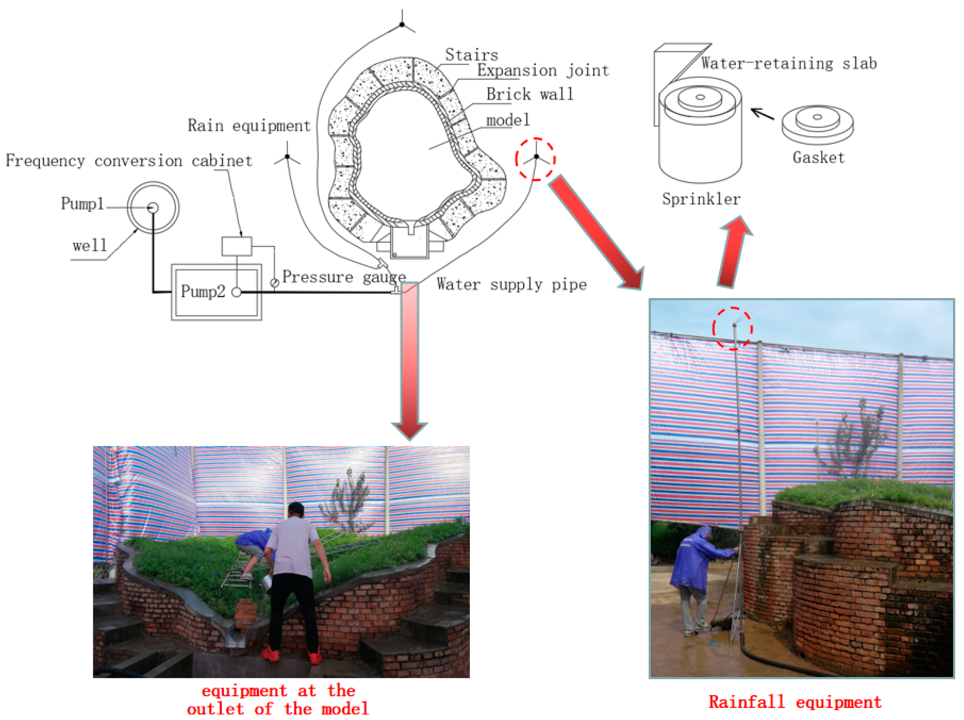
2.3. The Designed Rainfall

Extreme short-duration rain events were considered to be the main mechanism underlying the destruction of land consolidation projects. According to the statistical data, there have been 58 heavy rain events in Shaanxi Province since the 1960s in which the highest daily rainfall exceeded 200 mm. These events had the characteristics of short duration, high rainfall amount, and high intensity. The maximum 1 h rainfall ranged between 134 mm and 252 mm. The maximum 5 min rainfall ranged between 8.1 mm and 59.1 mm over nearly 200 observation stations on the Loess Plateau. Combined with the historical rainfall data collected in the Yan’an area and the historical runoff and sediment generation data collected in the Yangou small watershed, a maximum 6-h rainfall of 96.5 mm in 20 years was selected as the design rainfall. To keep the total rainfall of the watershed constant, six rainfall intensities were designed: 2 mm min⁻¹, 5 mm min⁻¹, 7 mm min⁻¹, 10 mm min⁻¹, 15 mm min⁻¹, and 20 mm min⁻¹. The designed rain intensity of the model was determined according to the rain intensity scale, where ${\lambda }_i$ = 10.

The rainfall simulation of the model mainly adopted artificial rainfall. The rainfall equipment was a BX-1 portable field rainfall device, and three groups were evenly arranged around the small watershed model. The rainfall equipment was composed of an adjustable tripod at the bottom, a stainless steel support rod in the middle, and a top sprinkler. The sprinkler was 8m from the ground and sprayed water at an elevation angle of 45° to keep the rainfall uniformity not less than 75%. The water supply source was groundwater near the model, and its water quality parameters had been measured for comparison and analysis in subsequent experiments. Two sets of water pumps were used for supply—pump 1 lifted the groundwater to the water tank for storage, and pump 2 was placed in the water tank and supplied water to the rainfall equipment through frequency conversion speed regulation (as shown in Figure 4).

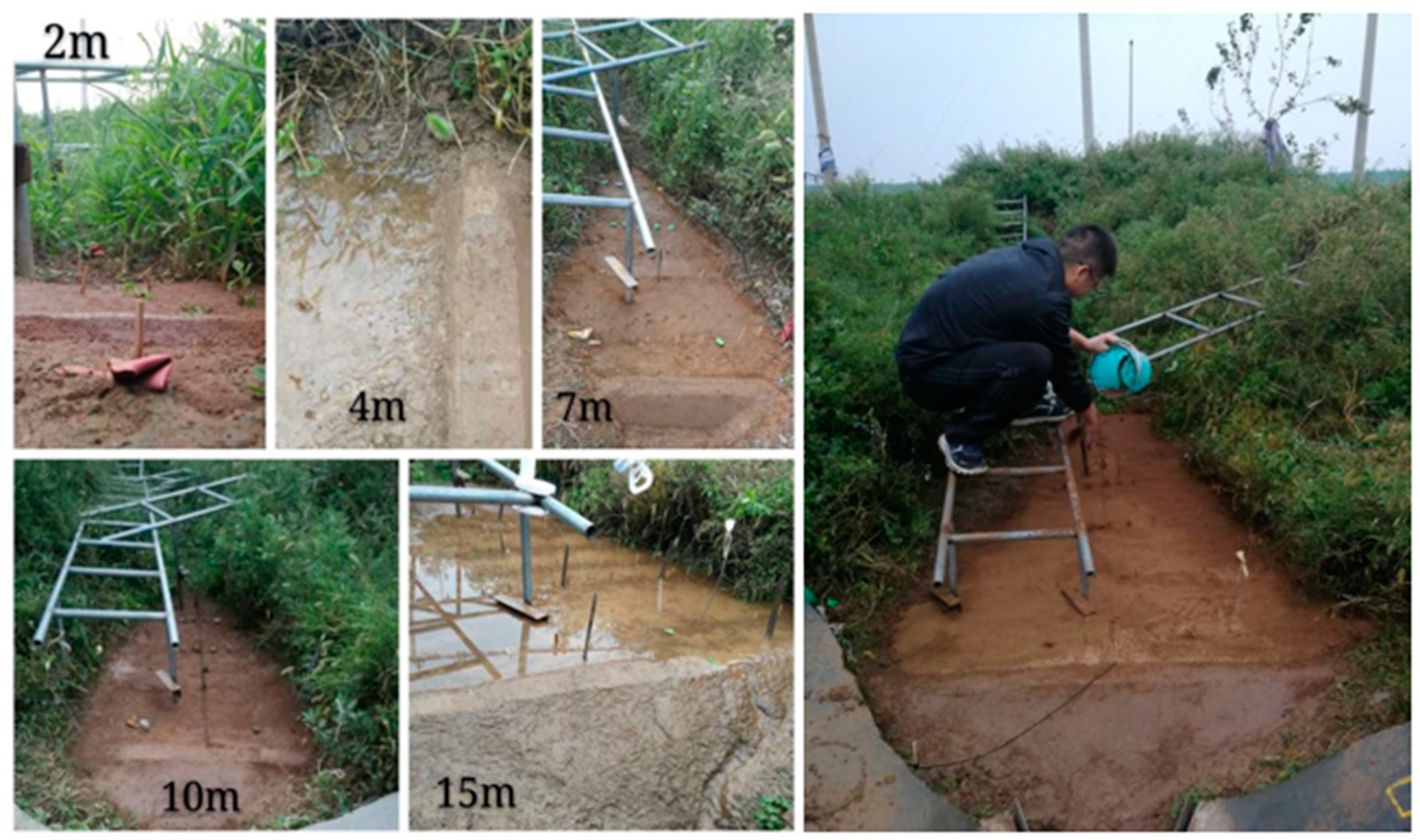
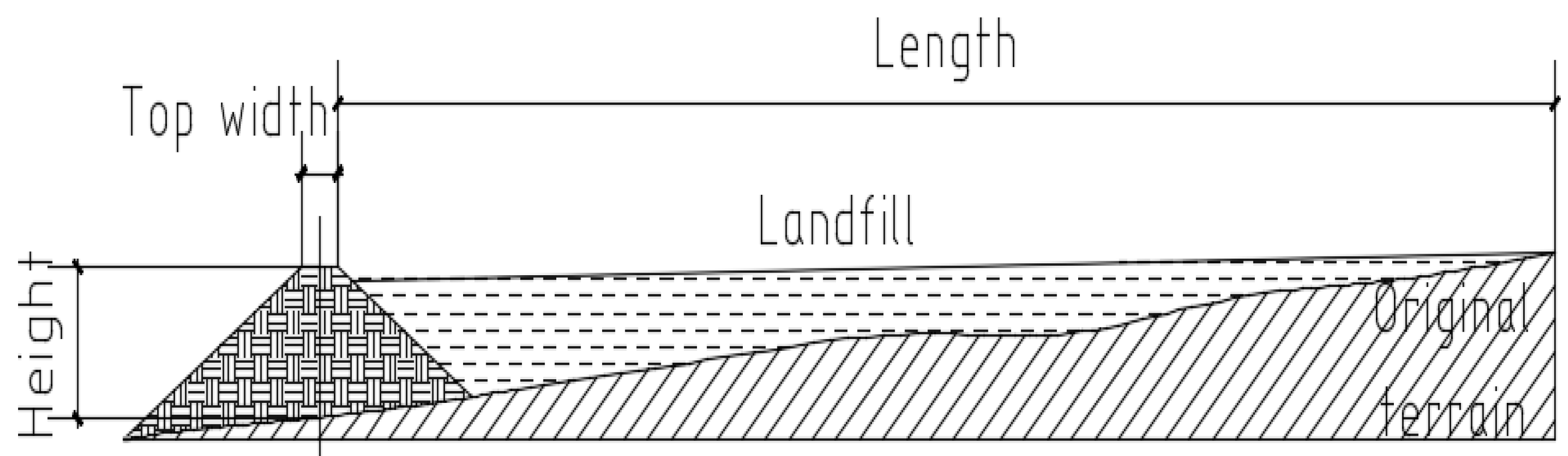
2.4. The Designed Land Consolidation

The study area contains a check dam. There have been almost no siltation changes due to the highly managed status of the watershed. This finding was consistent with the status of the GLCP in Yan’an. Thus, in the experiment, the scale of land consolidation was selected by varying the dam height, and as the height of the dam increased, the scale of land consolidation increased (as shown in Figure 5).

Table 3. Sectional dimensions of the prototype dam.

Dam Height (m)	Top Width (m)	Bottom Width (m)	Upstream Slope Ratio	Downstream Slope Ratio
2	1.5	6.3	1:1.2	1:1.2
4	2	14	1:1.5	1:1.5
7	2.5	23.5	1:1.5	1:1.5
10	3.5	33.5	1:1.5	1:1.5
15	4.5	49.5	1:1.5	1:1.5

shows the design height and related dimensions of the dam in the prototype small watershed, and Figure 6 shows the positions and construction methods corresponding to the dimensions in Table 3. In the simulation experiment, the sizes of the model dam and the land were converted according to the similar relationship in Table 2.

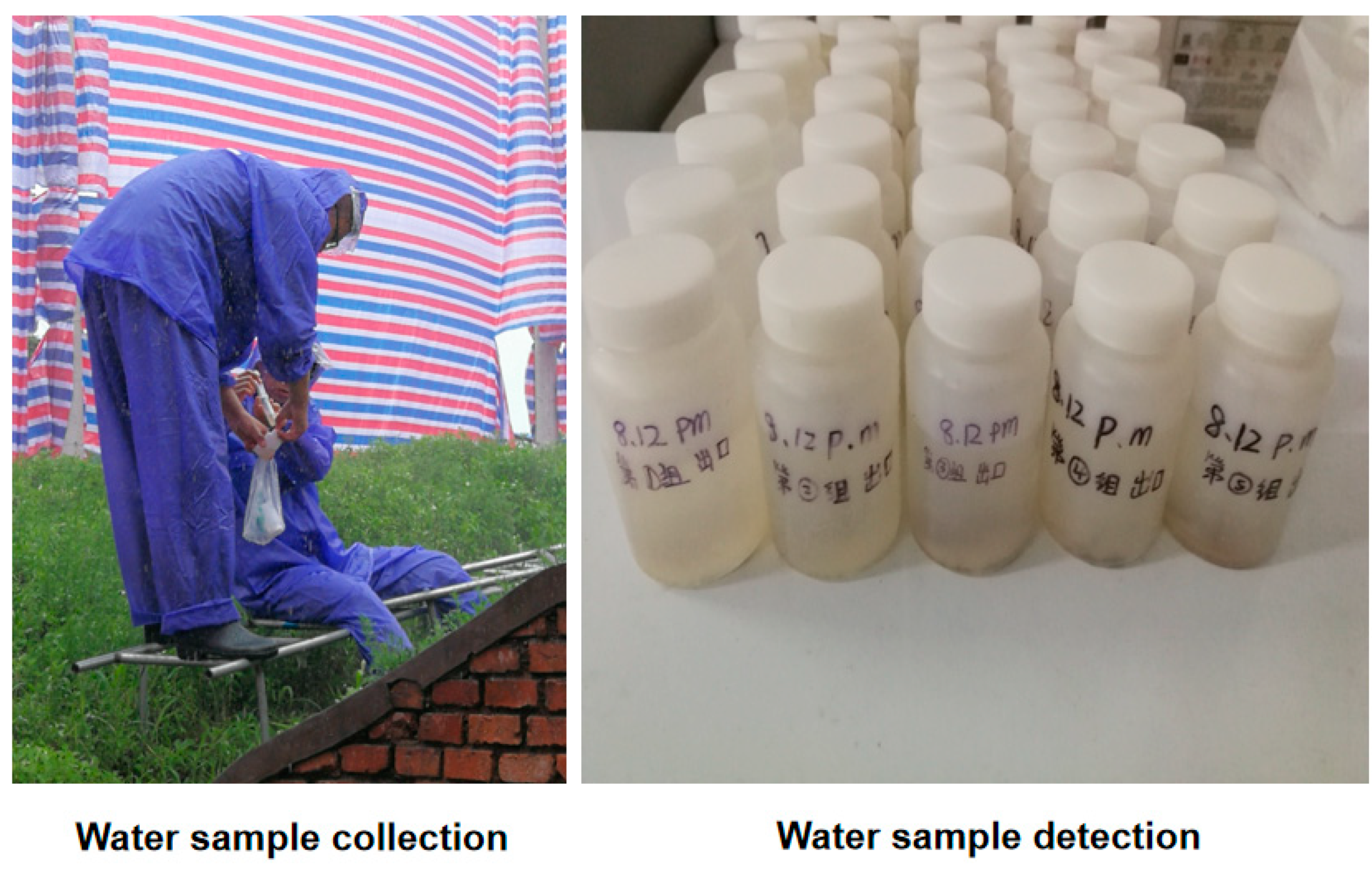
2.5. Data Collection

The times of rainfall onset and runoff generation were recorded. Runoff samples of a certain volume were collected at the outlet of the watershed at regular intervals using 20-cm diameter plastic buckets. The time of collecting runoff and the time spent in the collection process were recorded. Subsequently, a 100 mL plastic bottle was used to collect a certain amount of water samples at the outlet of the watershed and stored in refrigeration. We stirred the water sample in the plastic bucket evenly, measured its volume, poured it into the aluminum box with the corresponding number, and weighed the sediment after drying at 105 °C for 8 h, and then the sediments were analyzed for N, P, and K. The parameters such as flow rate and sediment content were calculated, respectively. The water sample in the plastic bottle was tested for its nitrogen and phosphorus content in the laboratory within 24 h (as shown in Figure 7).

While recording the outlet parameters of the watershed, the flow and sediment movement parameters in the gully were also measured. We set 5 measurement sections in the gully, and the relative distances (the ratio of the distance between the section to be measured and the starting point of the gully to the total length of the gully) from the beginning of the gully are: 0.42, 0.53, 0.64, 0.76 and 0.87. Furthermore, the water level and flow velocity of the section were measured, and the water and soil samples of each section were collected under specific rainfall conditions.

3. Results

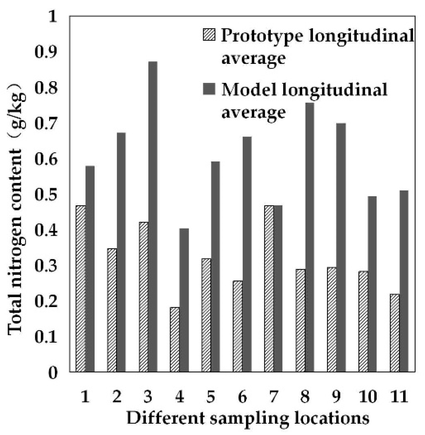
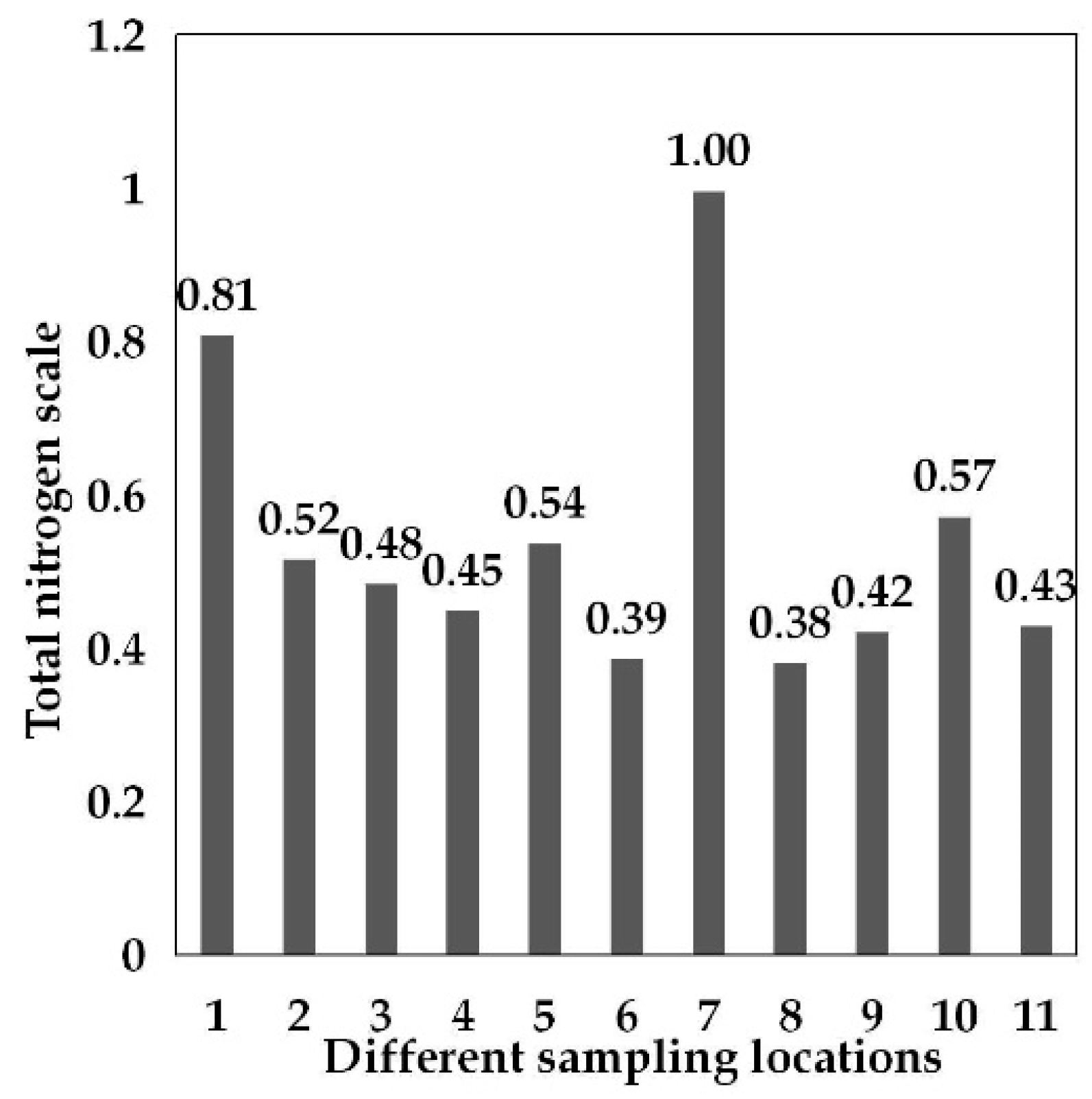
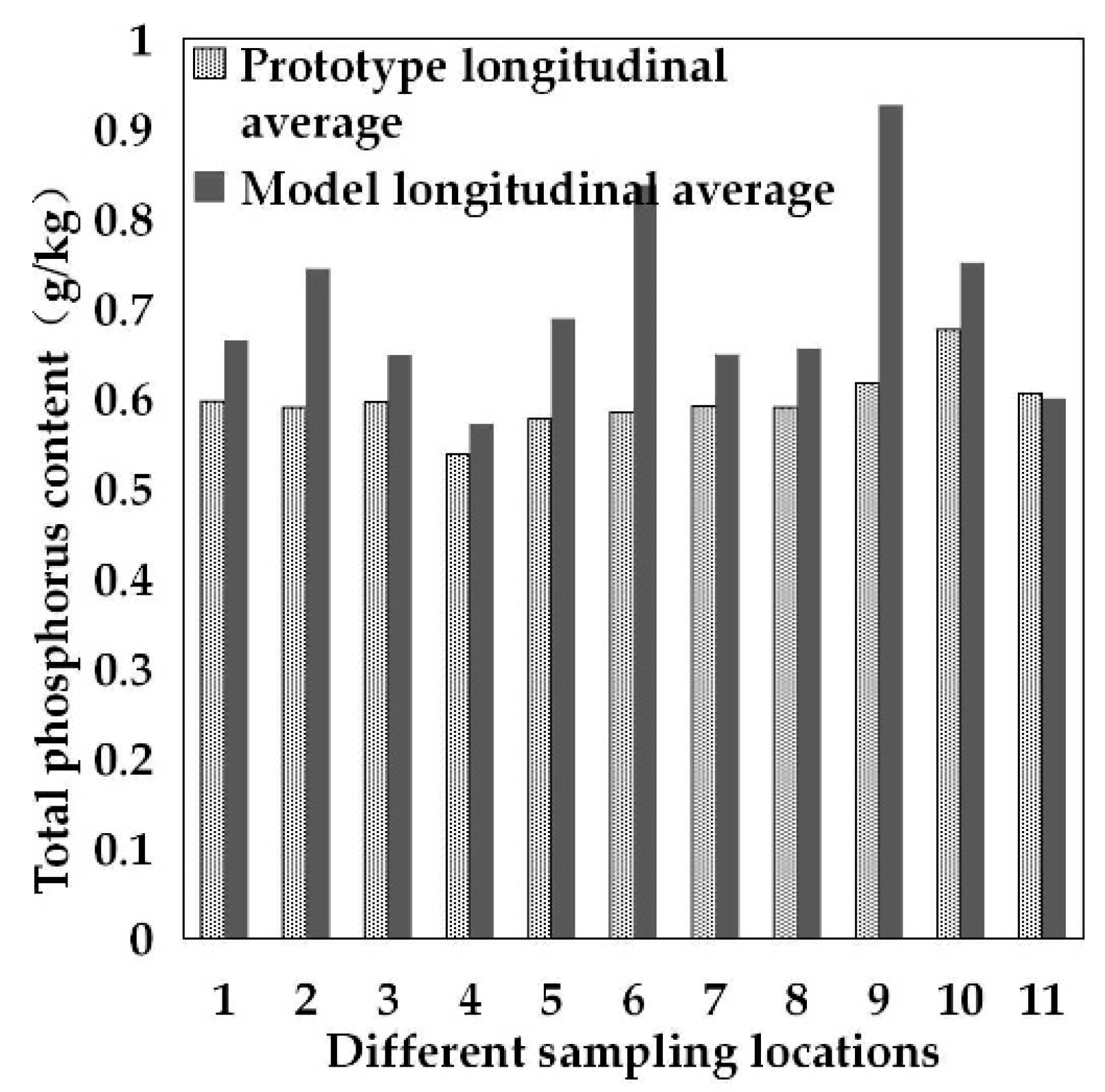
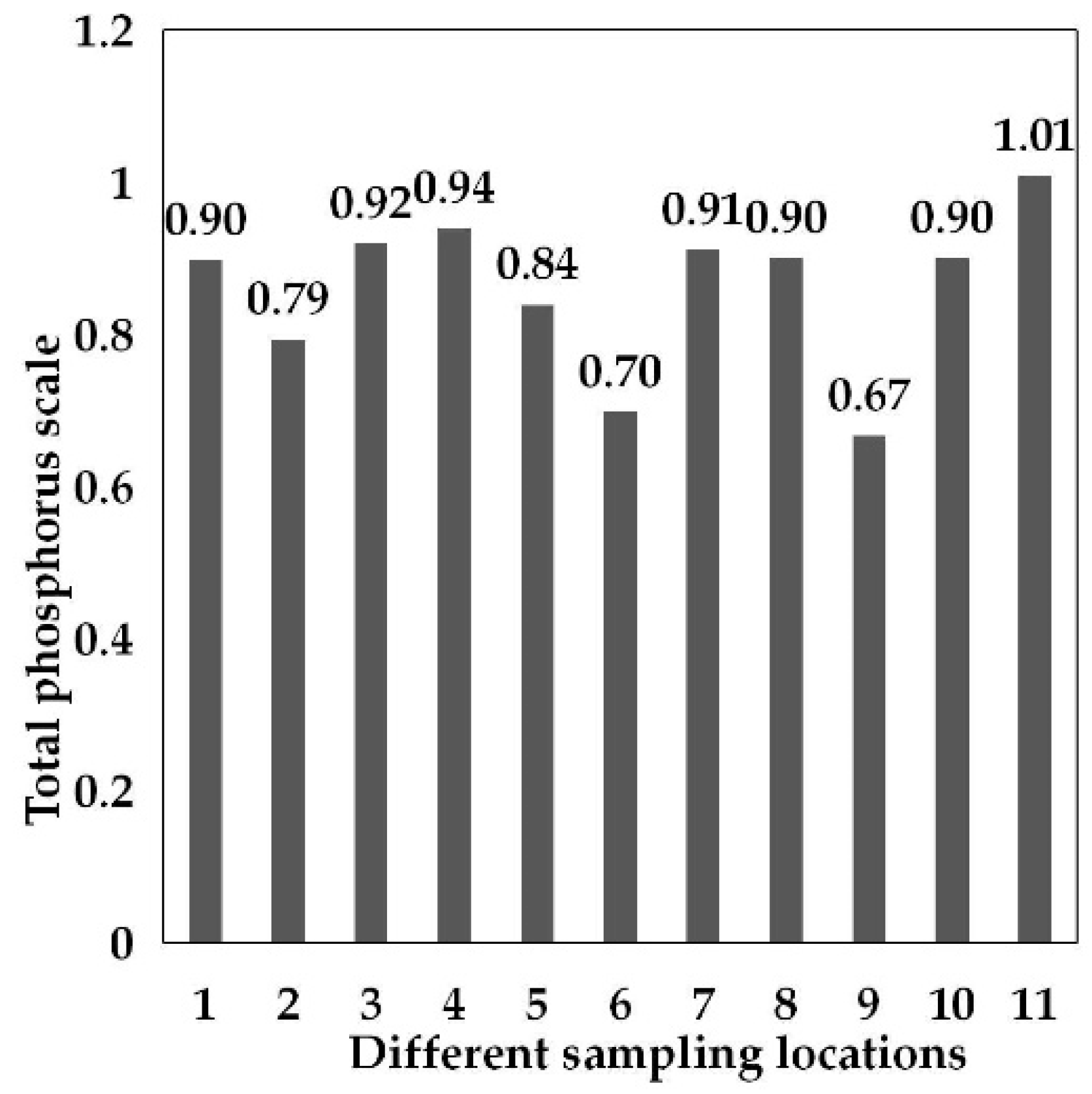
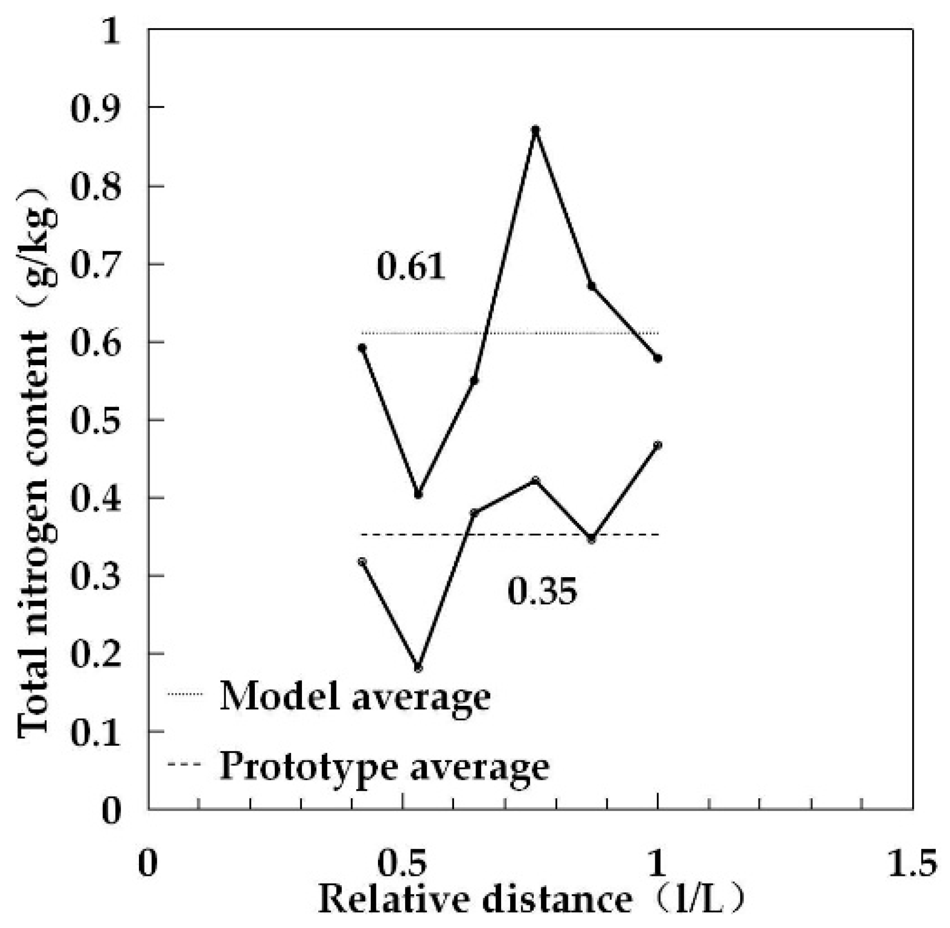
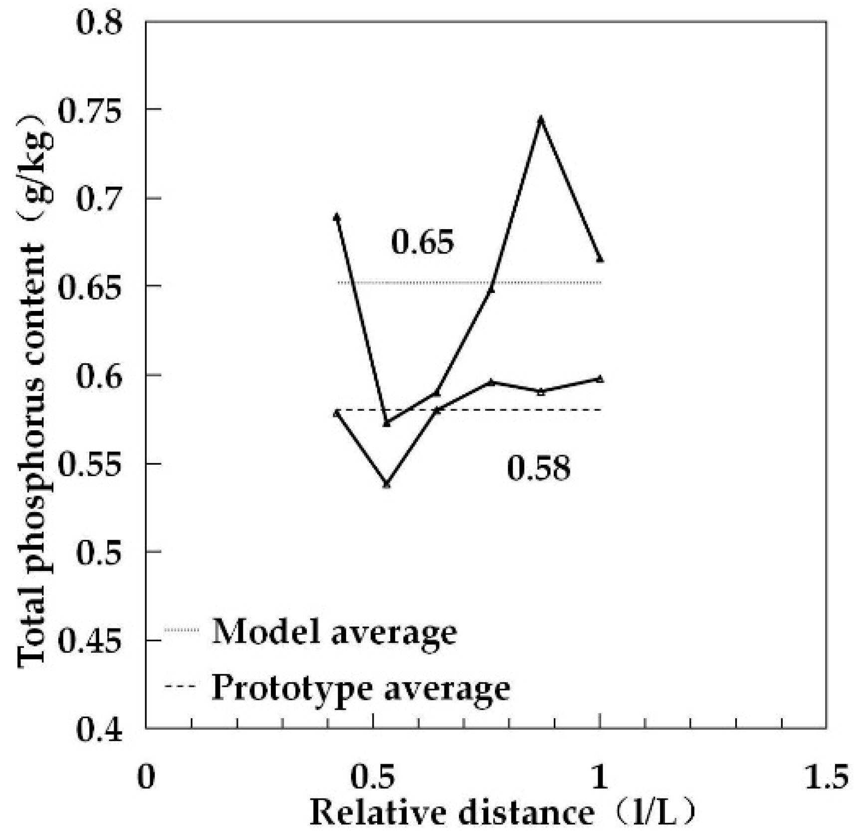
3.1. Determination of Pollutant Scale and Verification

In order to study the influence of rainfall–runoff processes on pollutant contents in small watersheds, it is necessary to explore the transport patterns of non-point source pollution in watersheds under different rainfall events and land consolidation proportions. However, the transportation of the nonpoint source pollution caused by erosion in the study area was so complicated that an appropriate new method was developed. Based on the similarity principle, soil samples of different depths were extracted from 11 corresponding sampling points of the prototype and model, the nitrogen and phosphorus contents in each soil sample were measured, and the longitudinal average value was taken as the nitrogen and phosphorus content of the sampling point. The content ratios of the corresponding points are shown in Figure 8, Figure 9, Figure 10 and Figure 11. Figure 8 and Figure 9 indicate that the initial nitrogen content scale was ${\lambda }_{\mathrm{Nm}} = 0.5$, and Figure 10 and Figure 11 indicate that the initial phosphorus content scale was ${\lambda }_{Pm} = 0.9$.

The model test was run under the conditions of equivalent rainfall intensity I_m = 0.114 mm min⁻¹ and rainfall time T_m = 37.5 min. After each rainfall event, soil samples were taken along the channel for measurement. The average nitrogen and phosphorus contents in the channel soil, modeled as a function of relative distance, were compared with the corresponding parameters of the prototype at each position, as shown in Figure 12 and Figure 13. The figures show that the average content of pollutant nitrogen in the prototype and model soils was 0.35 g kg⁻¹ and 0.61 g kg⁻¹, respectively. The pollutant nitrogen content scale was 0.57, which was approximately equal to the derived nitrogen content scale ${\lambda }_{Nc} = 0.5$. The average content of phosphorus in the prototype and modeled soils was 0.58 g kg⁻¹ and 0.65 g kg⁻¹, respectively. The pollutant phosphorus content scale was 0.89, which was approximately equal to the derived phosphorus content scale ${\lambda }_{Pc} = 0.9$, verifying the pollutant content similarity between the prototype and model.

Based on the determination and verification of the pollutant scale as described above, a complete set of small-watershed scale model similarity values was obtained, as presented in Table 2. Table 2 indicates the similarity conversion relationships of rainfall, runoff, eroded sediment, and pollutant transportation. The table also demonstrates the similarity in rainfall–runoff erosion environments required to satisfy the similarities in geometry, rainfall, vegetation cover, water flow movement, erosion sediment movement, and pollutant transport.

3.2. The Impact of Vegetation Restoration on Erosion Transport in Small Watersheds

At present, the vegetation coverage of the Kangjiagelao watershed in Yangou has reached 90% of the total area. Based on the completion of the rainfall runoff erosion and sediment transport test under bare land conditions and the determination and verification of the pollutant transport scale in the current basin, a comparative study was carried out for the changes in runoff and sediment yield, land-use and erosion control before and after vegetation restoration in the small watershed.

The hydrological process of slope surface runoff is an important factor influencing erosion and is driven by extreme rainstorms. To explore the impact of vegetation restoration on erosion transport, five rainfall events with intensities of 1.14 mm min⁻¹, 5 mm min⁻¹, 10 mm min⁻¹, 15 mm min⁻¹, and 20 mm min⁻¹ were performed before and after vegetation restoration. The parameters included runoff generation time, peak flood discharge time, peak flood discharge value, peak sediment discharge time, peak sediment discharge value, and erosion modulus. In addition, the changes in watershed outlet flow and sediment content with time before and after vegetation restoration were analyzed. The results are shown in Figure 14, Figure 15, Figure 16, Figure 17, Figure 18 and Figure 19 and

Table 4. Parameters of runoff and sediment generation in small watersheds, before and after vegetation restoration.

Runoff or Sediment Movement Parameter	Before Vegetation Restoration	After Vegetation Restoration
Runoff generation time (tc)	$t_c^{\prime } = 18.13\times {10}^{-0.04i}$	$t_c^{"} = 77.9\times {10}^{-0.05i}$
Peak flood discharge time (th)	$t_h^{\prime } = 118.7\times {10}^{-0.013i}$	$t_h^{"} = 315.1\times {10}^{-0.017i}$
Peak flood discharge (Qh)	$Q_h^{\prime } = 4.5\times {10}^{0.05i}$	$Q_h^{"} = 0.29\times {10}^{0.12i}$
Peak sediment discharge time (ts)	$t_s^{\prime } = 120.8\times {10}^{-0.02i}$	$t_s^{"} = 299\times {10}^{-0.03i}$
Erosion modulus (E)	$E^{\prime } = 2919.4\times {10}^{0.03i}$	$E^{″} = 1.54\times {10}^{0.06i}$
Peak sediment discharge value (Sf)	$S_f^{\prime } = 104.9\times {10}^{0.01i}$	$S_f^{"} = 0.59\times {10}^{0.05i}$

.

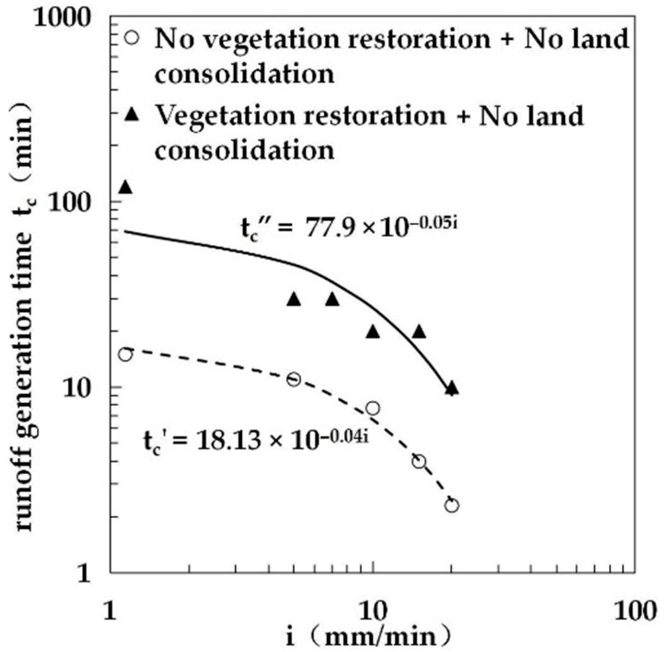
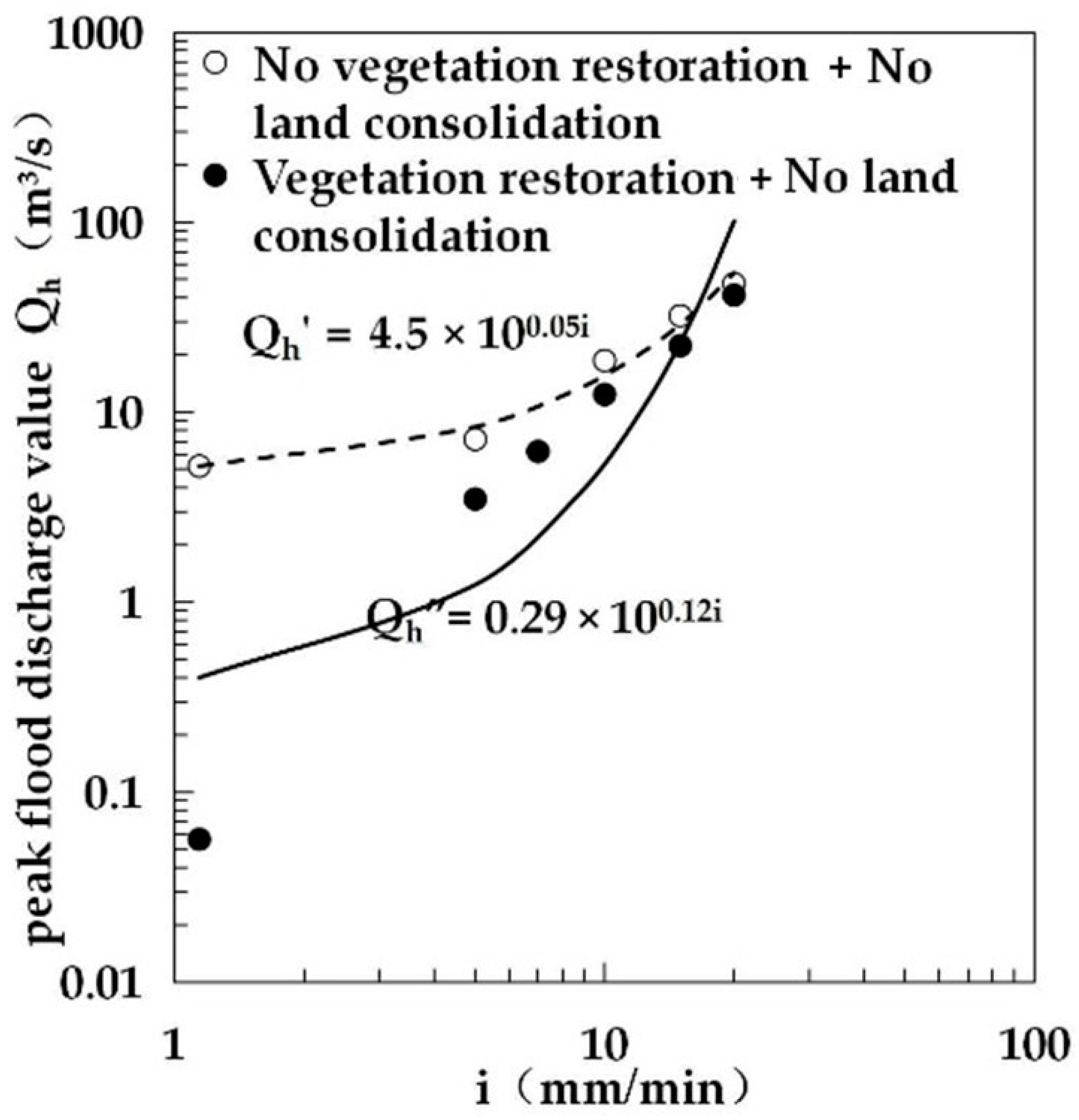
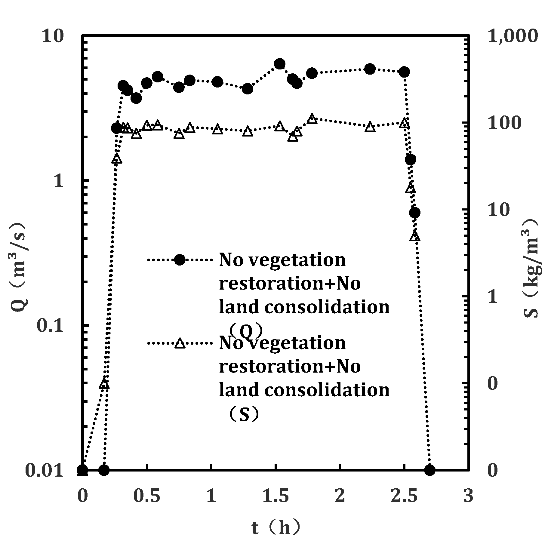
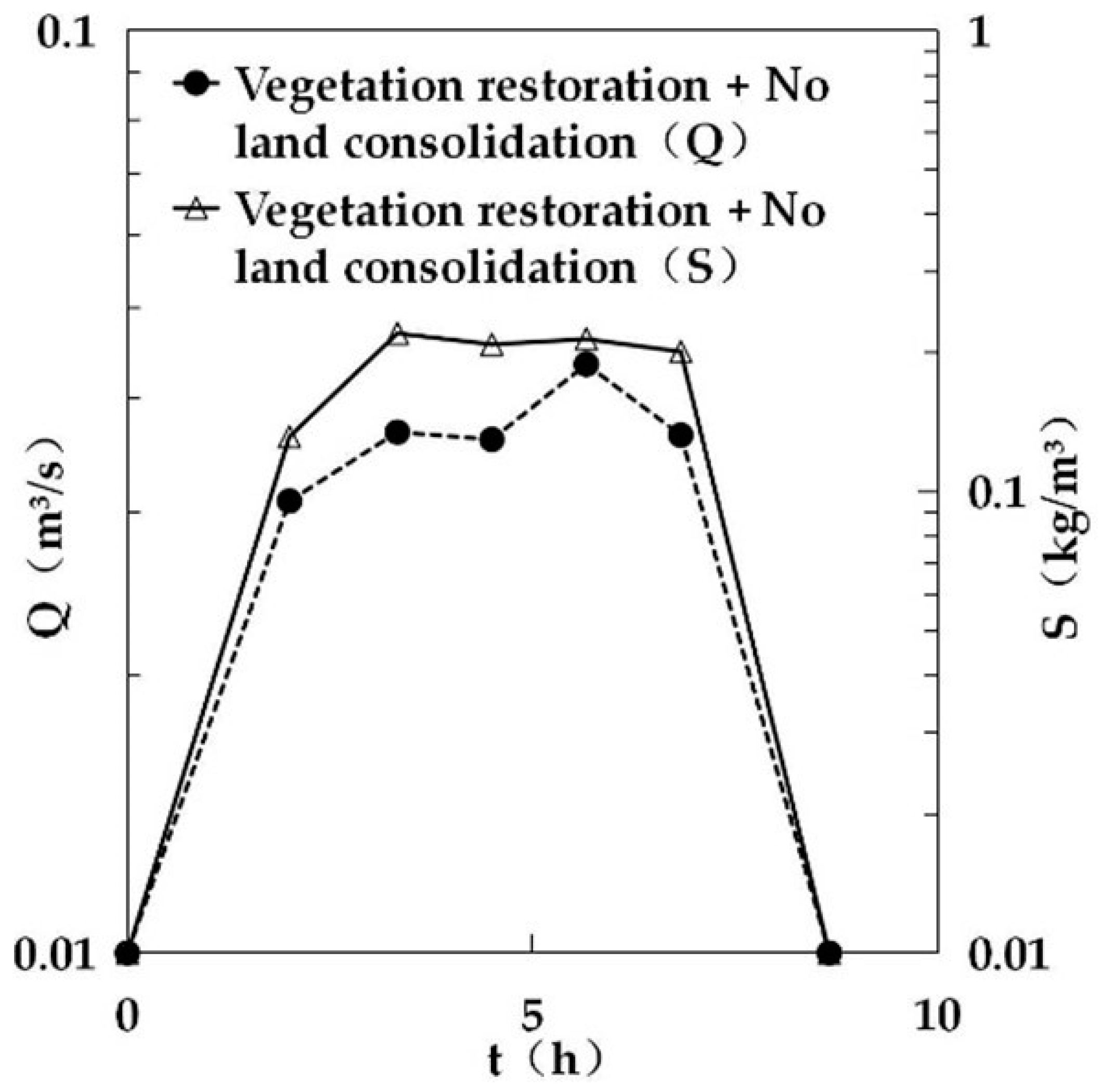
3.2.1. The Impacts of Vegetation Restoration on Runoff Generation and Collection

Vegetation restoration had important effects on the time of runoff generation. Figure 14 shows the changes in runoff generation time (t_c) with rain intensity (i) before and after vegetation restoration. It could be seen from the figure that the change trend of runoff generation time before and after vegetation restoration was the same, and both decreased with an increased rainfall intensity. However, the change trend of runoff generation time after vegetation restoration was more obvious than before. The formula coefficient increased by 4.3 times after vegetation restoration in delaying time to runoff generation under all rainfall intensities. After vegetation restoration, the average time to runoff generation was delayed by 330% relative to before the restoration. The changes in flood peak discharge time with rainfall intensity showed similar trends, as shown in Table 4. Figure 15 shows the changes in flood peak discharge (Q_h) as a function of rainfall intensity (i). Although the flood peak discharge increased with increasing rainfall intensity, it decreased significantly after vegetation restoration, and the rate of increase in flood peak discharge with rainfall intensity was greater in after vegetation than before vegetation. It was theoretically possible to exceed the flood peak discharge before vegetation under heavy rainfall, indicating that the effect of vegetation on runoff reduction was limited. When the rainfall intensity exceeded 10 mm min⁻¹, the flood peak discharge after vegetation was greater than before, and this phenomenon has been observed previously, both at home and abroad. These findings were highly significant for the design of flood control practices under extreme rainfall conditions.

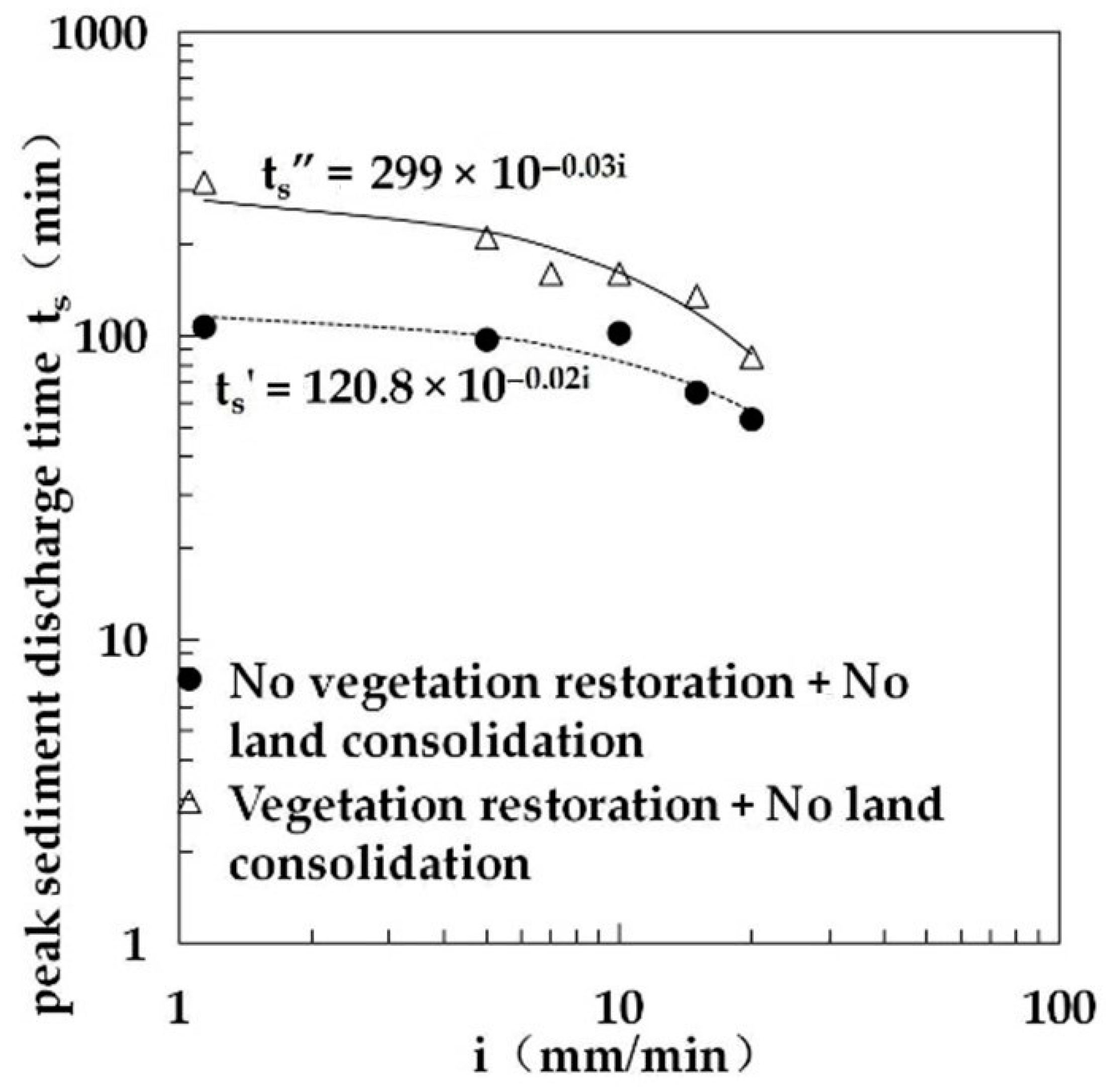
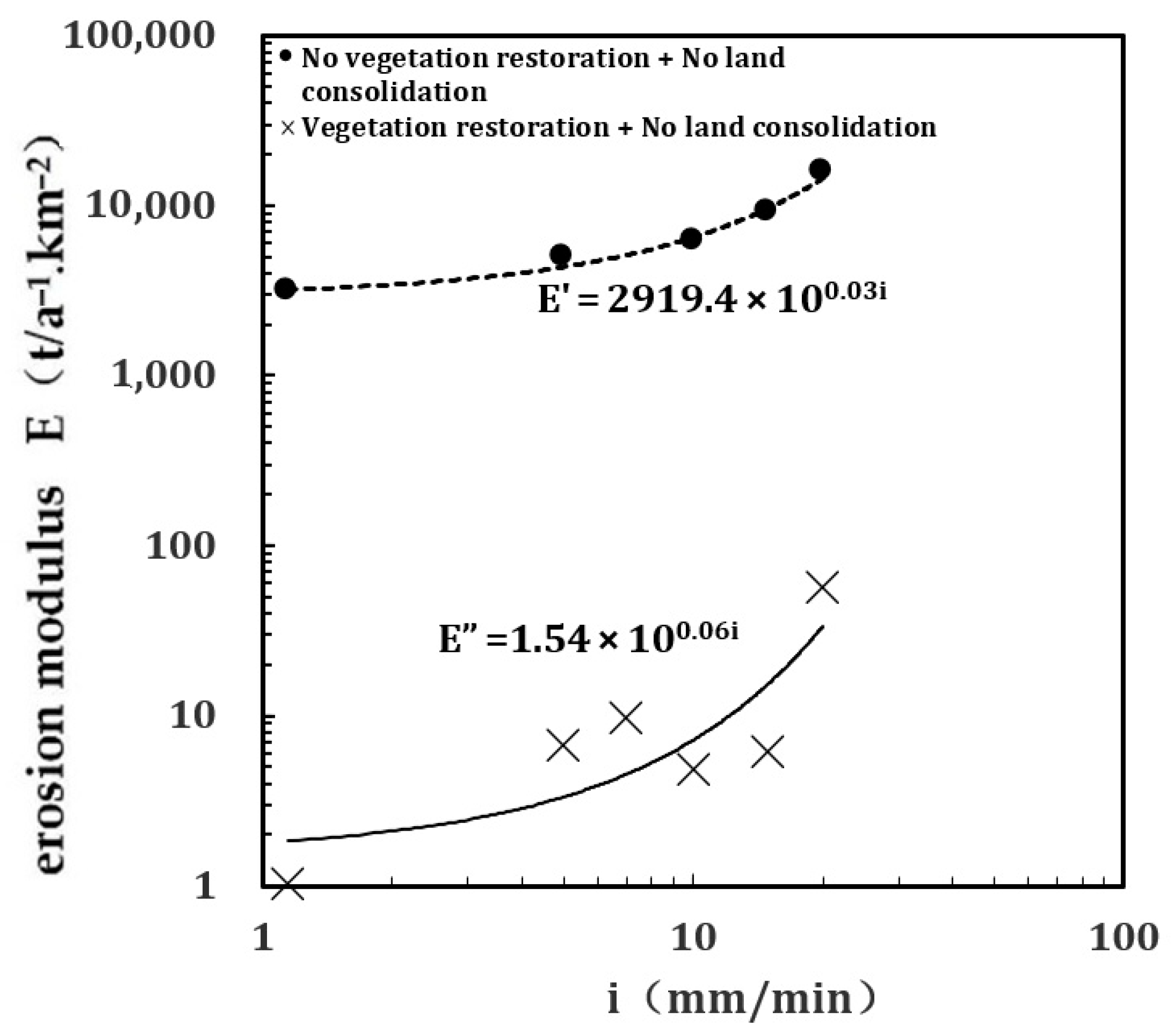
3.2.2. The Impact of Vegetation Restoration on Eroded Sediment Generation

Vegetation restoration had an important effect on the transport of eroded sediment. Figure 16 shows the changes in sediment peak discharge time (t_s) as a function of rain intensity (i). The sediment peak discharge time decreased with increasing rainfall intensity before and after vegetation restoration. The average sediment peak discharge time after vegetation restoration was 2.48 times longer than before vegetation restoration. Figure 17 shows the changes in erosion modulus with rainfall intensity before and after vegetation restoration, under the condition of a prototype-equivalent total rainfall of 150 mm. The results showed that the erosion modulus increased with increasing rain intensity before and after vegetation restoration, and that the erosion modulus of the small watershed clearly decreased after vegetation restoration. However, the erosion modulus increased at an increasingly fast rate as rainfall intensity increased, suggesting that it was able to increase the erosional transport volume at a certain rainfall intensity. A possible explanation for this finding could be that gravitational erosion increases with increasing rainfall intensity. The changes in sediment peak discharge with rain intensity before and after vegetation restoration exhibited similar characteristics, as presented in Table 4.

3.2.3. The Impact of Vegetation Restoration on the Relationship between Runoff and Sediment Generation

Vegetation restoration had an important influence on the relationship between runoff and sediment production and affected the runoff driving mechanisms. Among the five sets of prototype-designed rainfall intensities, a typical prototype’s maximum at 10-min rainfall intensity of 1.14 mm min⁻¹, with a return period of 2 years, was selected as the experimental rainfall intensity, and the changes in runoff and sediment content over time at the outlet of the watershed before and after vegetation restoration were compared, as shown in Figure 18 and Figure 19. The figures show that before vegetation restoration, the surface runoff stabilization time after runoff generation was 20 min, the average discharge after stabilization was 4.92 m³ s⁻¹, the average sediment content was 87.3 kg/m³, the flood peak discharge was 6.4 m³/s, the flood peak time was 91.8 min, the sediment peak discharge value was 112 kg m⁻³, and the sediment peak discharge time was 106.8 min. After vegetation restoration, the flow stabilization after surface runoff generation occurred at 120 min, the average discharge after stabilization was 0.036 m³ s⁻¹, the average sediment content was 0.21 kg m⁻³, the flood peak discharge was 0.043 m³ s⁻¹, the flood peak time was 336 min, the peak sediment discharge value was 0.22 kg m⁻³, and the peak sediment time was 200 min.

The above results showed that the runoff and sediment generation times clearly reduced and the amount of runoff and sediment was significantly reduced after vegetation restoration. These results indicated that the vegetation measures taken had positive impacts on soil and water conservation. Additionally, this experiment showed that the sediment peak discharge occurred at the front while the flood peak occurred at the back when watersheds were highly managed. These findings were important as they indicated a change in the runoff production mechanism, and new topics have been proposed for flood control and early warning—especially the variation points of vegetation coverage need further study.

3.3. The Influence of Land Consolidation on Erosion Transport

To explore the impact of land consolidation projects on erosion transport in small watersheds, experiments were performed with six rain intensities, 1.14 mm min⁻¹, 5 mm min⁻¹, 7 mm min⁻¹, 10 mm min⁻¹, 15 mm min⁻¹ and 20 mm min⁻¹, and five land consolidation proportions, 0.47%, 0.85%, 2.00%, 3.30% and 6.13%. The changes in runoff and sediment movement were comprehensively analyzed under the various land consolidation proportions and rainfall intensities for the 90% managed watershed, as shown in Figure 20, Figure 21, Figure 22, Figure 23, Figure 24, Figure 25, Figure 26, Figure 27 and Figure 28.

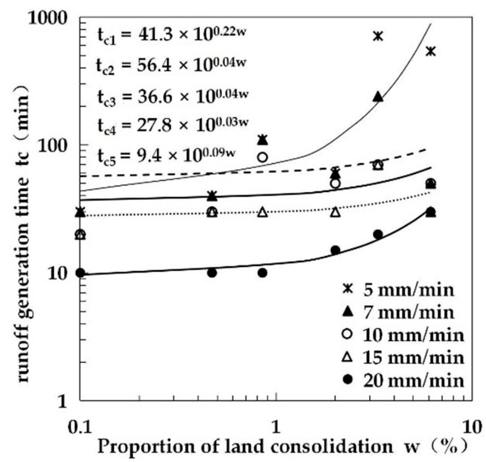
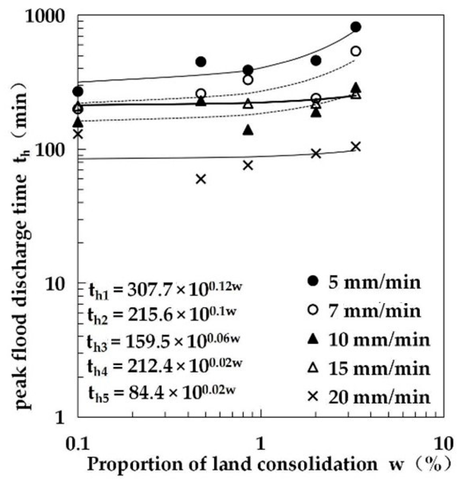
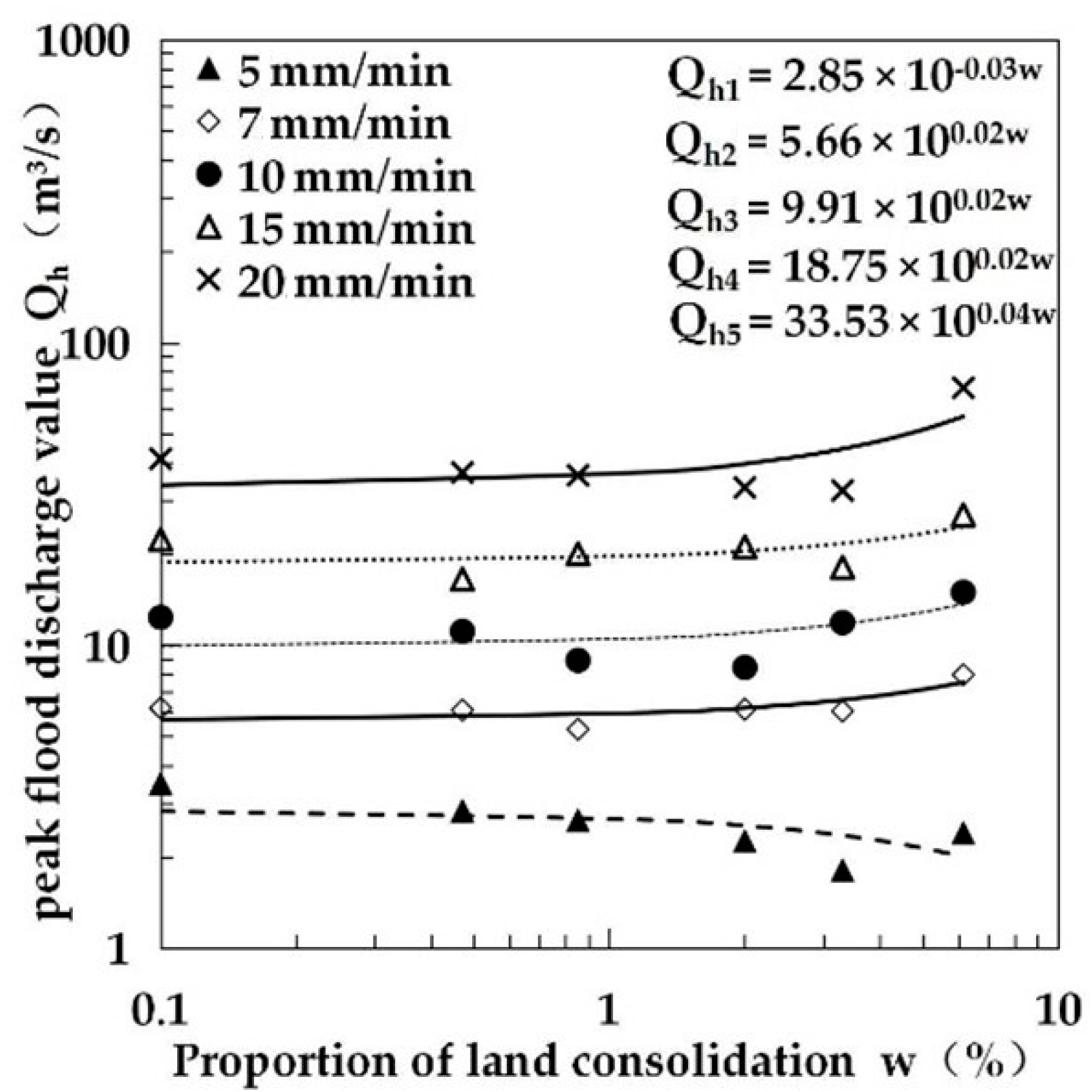
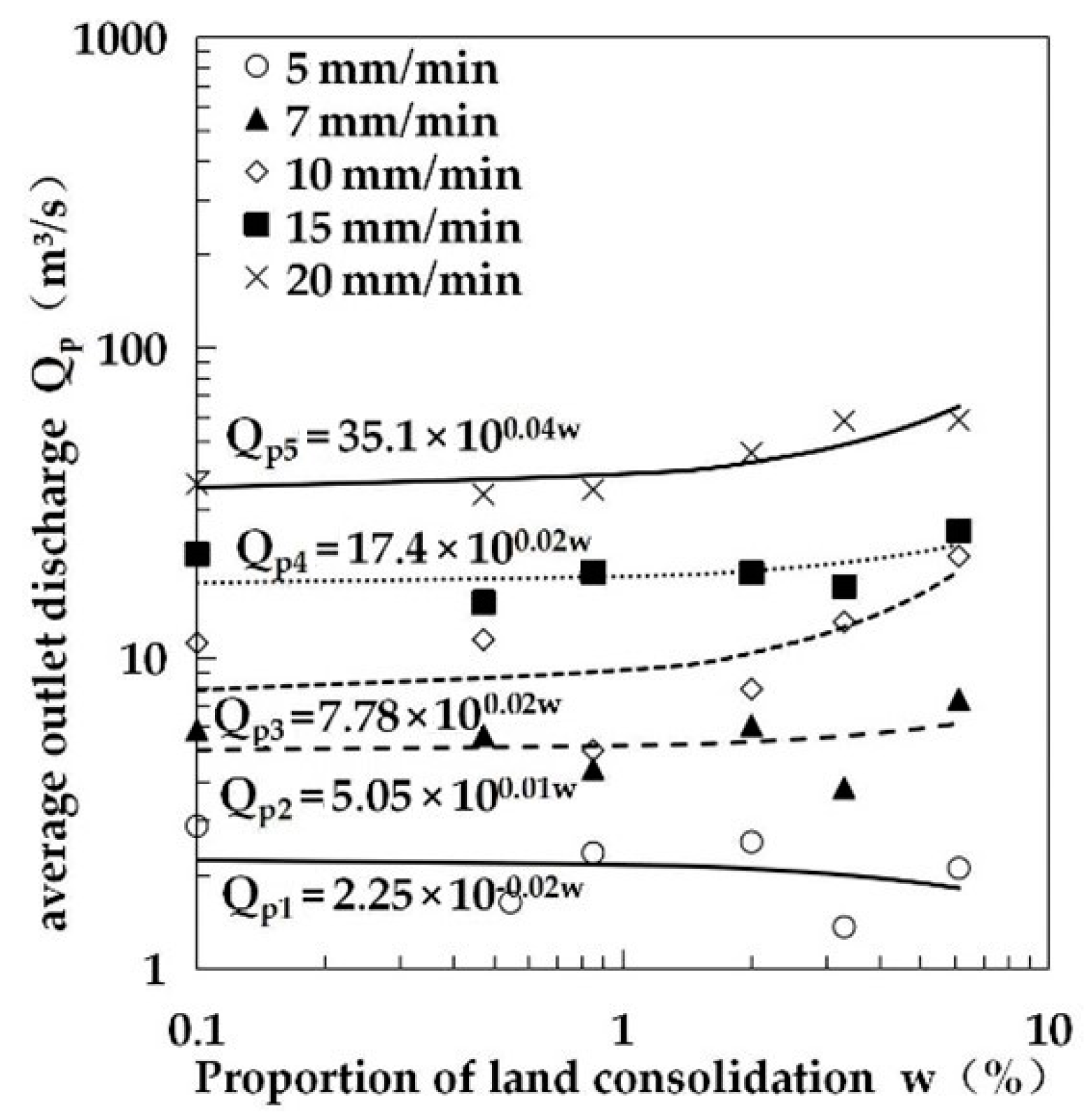
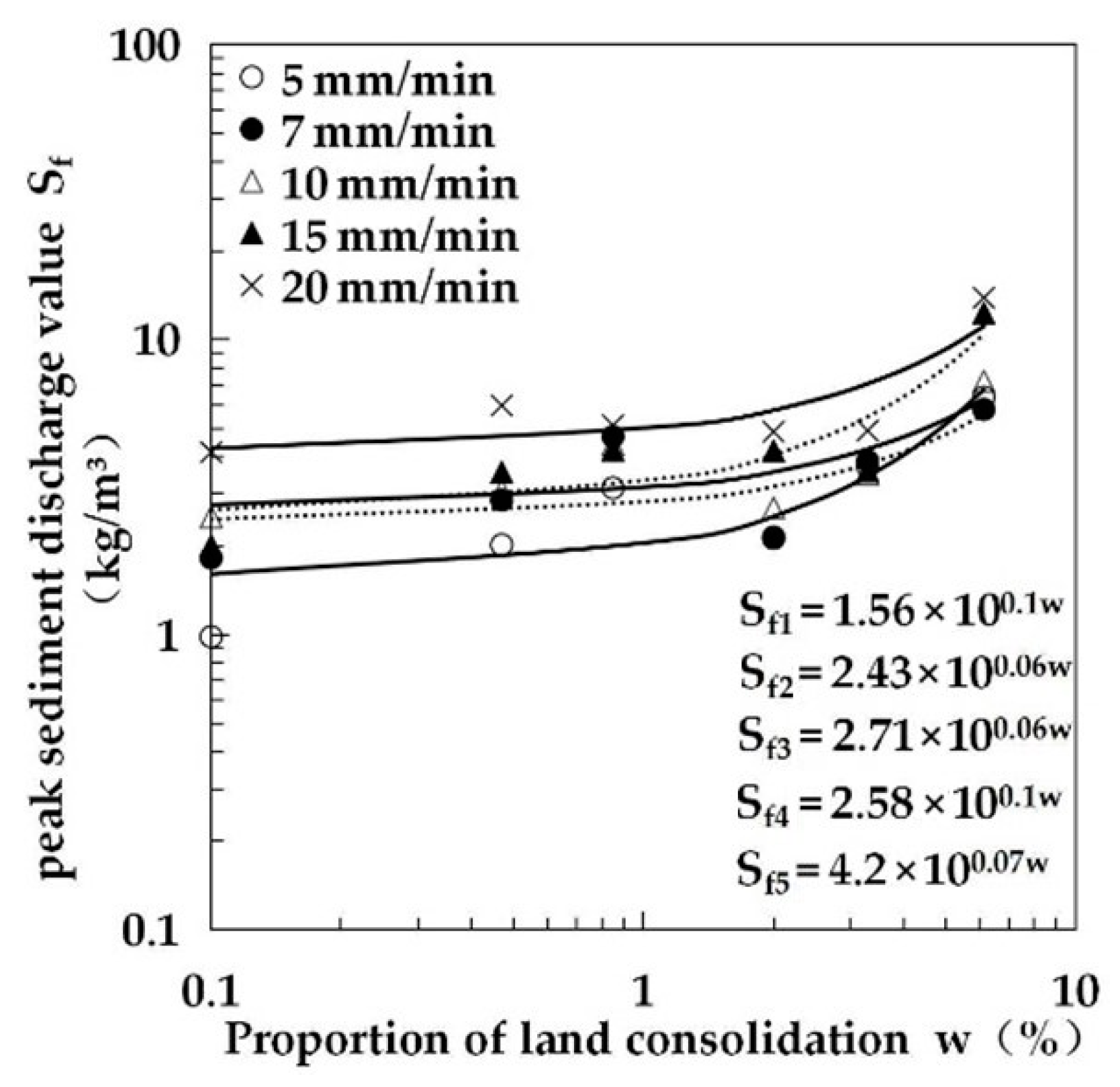
3.3.1. The Impacts on Runoff and Sediment Generation

Due to the different proportions of land consolidation in the gully, the degree of impact on the erosion and transport of water and sediment is also different. The low rainfall intensity of 1.14 mm min⁻¹ did not produce runoff in most land consolidation cases and hence the analyses predominantly considered data for the rain intensities of 5–20 mm min⁻¹. Figure 20 shows that the runoff generation time for each rain intensity level increased with increasing land consolidation proportion, and the runoff generation time under each consolidation proportion was delayed in comparison to without consolidation. These results demonstrated that land consolidation projects with different proportions exhibited varied effects on the runoff generation time of small watersheds. A greater consolidation proportion and lower rainfall intensity corresponded to a longer runoff generation time. When the proportion of land consolidation was less than 0.85%, the runoff generation time shifted smoothly and land consolidation had little effect on runoff generation in the watershed—when the proportion was between 0.85% and 3.3%, it would have varying degrees of impact on the runoff generation time under different rain intensities, and when it was greater than 3.3%, the runoff generation time changed significantly.

Figure 21 shows the influences of the land consolidation projects of different scales on peak flood discharge time. The results indicate that the flood peak time is proportional to the land consolidation proportion and all land consolidation projects delay flood peak time. The greater the consolidation proportion, the more obvious the effect of flood peak time. The main reason for this pattern is that an increase in the proportion of land consolidation results in increases in land area and infiltration. The variation point of flood peak time was approximately 2% of the consolidation proportion.

Figure 22 and Figure 23 indicate variations in flood peak and average discharge under different land consolidation proportions and rainfall intensities. The figures show that when the rain intensity was less than or equal to 5 mm min⁻¹, flood peak discharge and average outlet discharge decreased with increasing consolidation proportion and the land consolidation projects reduced the flood peak discharge and average outlet discharge. When the rain intensity exceeded 5 mm min⁻¹ and the land consolidation proportion was greater than 0.85%, both flood peak discharge and average discharge increased with increasing consolidation proportion, and when the consolidation proportion exceeded 3.3%, the changes gradually intensified. These results indicated that flood peak discharge and erosion in highly managed watersheds can be expected to increase sharply when the exposed area exceeds 3.3%; therefore, the proportion of land consolidation should not exceed 3.3%.

Figure 24 shows the influence of land consolidation projects of different scales on sediment peak discharge time. In the figure, it can be seen that the sediment peak discharge time curves are almost horizontal and there was little influence on the sediment peak discharge times in the range of 0 to 0.85% of land consolidation proportion. When the rainfall intensity was less than or equal to 5–7 mm min⁻¹, the peak sediment discharge time increased with increasing land consolidation proportion. This finding indicated that the land consolidation project increased infiltration and reduced runoff and erosion, which delayed the arrival time of the sediment peak discharge and a higher consolidation ratio resulted in a more obvious effect. When the rain intensity exceeded 5–7 mm min⁻¹, the sediment peak discharge time decreased with increasing consolidation proportion. Generally speaking, when the land consolidation proportion was less than 0.85%, the change in sediment peak discharge time was not obvious compared with an unmanaged watershed. When the land consolidation proportion was between 0.85 and 3.3%, the sediment peak discharge time changed differently under different rainfall intensities. When the consolidation proportion exceeded 3.3%, the sediment peak discharge time changed drastically, especially when the rain intensity was high, for instance, a sharp decrease in sediment peak discharge time occurred and the sediment peak discharge appeared early, indicating an increase in erosion.

Figure 25, Figure 26 and Figure 27 show the changes in the sediment peak discharge value, average outlet sediment content, and average outlet sediment transport ratio for the small watersheds with different land consolidation proportions and rainfall intensities. In all figures, the curves were nearly horizontal between 0% and 0.85% land consolidation proportions, and when the consolidation proportion was between 0.85% and 3.3%, the sediment peak discharge, average sediment content, and the average sediment transport ratio exhibited a slow rise with the increase in the land consolidation proportion. However, when the proportion was greater than 3.3%, most of the curves showed significant upward trends with increasing land consolidation proportion. Therefore, no more than 3.3% of land consolidation proportion should be critical for controlling sediment transport for HMSW.

Furthermore, a small watershed-scale simulation test was conducted under the conditions of a 150-mm prototype-equivalent rainfall and six rain intensities of 1.14 mm min⁻¹, 5 mm min⁻¹, 7 mm min., 10 mm min⁻¹, 15 mm min⁻¹, and 20 mm min⁻¹ to obtain the changes in the erosion modulus under different land consolidation conditions, as shown in Figure 28. The trends of these curves were similar to those above: the consolidation proportions less than 0.85%, between 0.85 and 3.3%, and greater than 3.3% correspond to different degrees of changes, and are the thresholds for the land consolidation proportion.

In summary, the critical value of the land consolidation proportion was established for the highly managed watershed. When the threshold was exceeded, the erosion obviously increased and the environment deteriorated. In the Kangjia watershed with 90% coverage, the proportion of GLCP should not exceed 3.3%, since when it was between 0.85% and 3.3%, the impact was not too great.

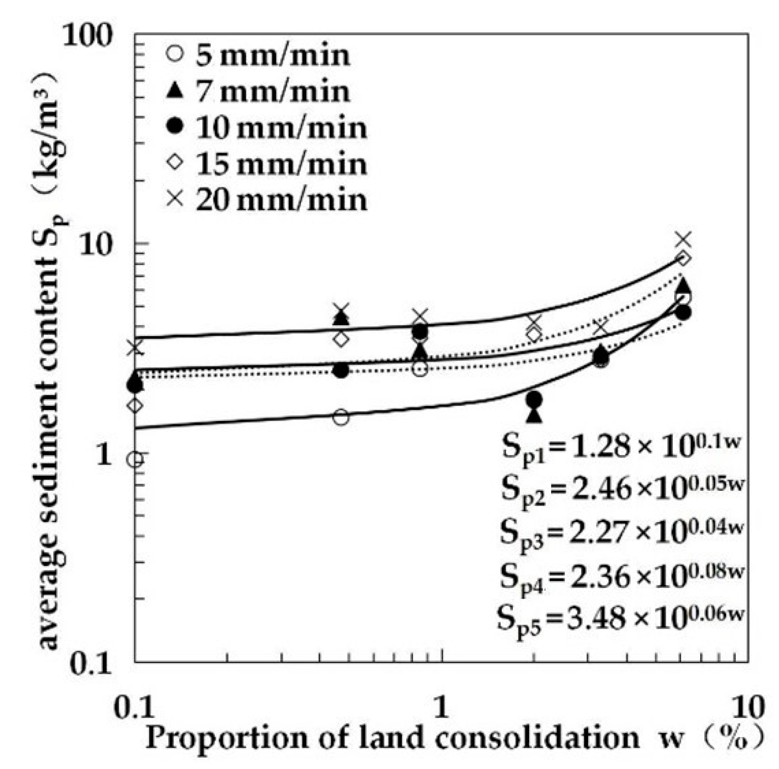
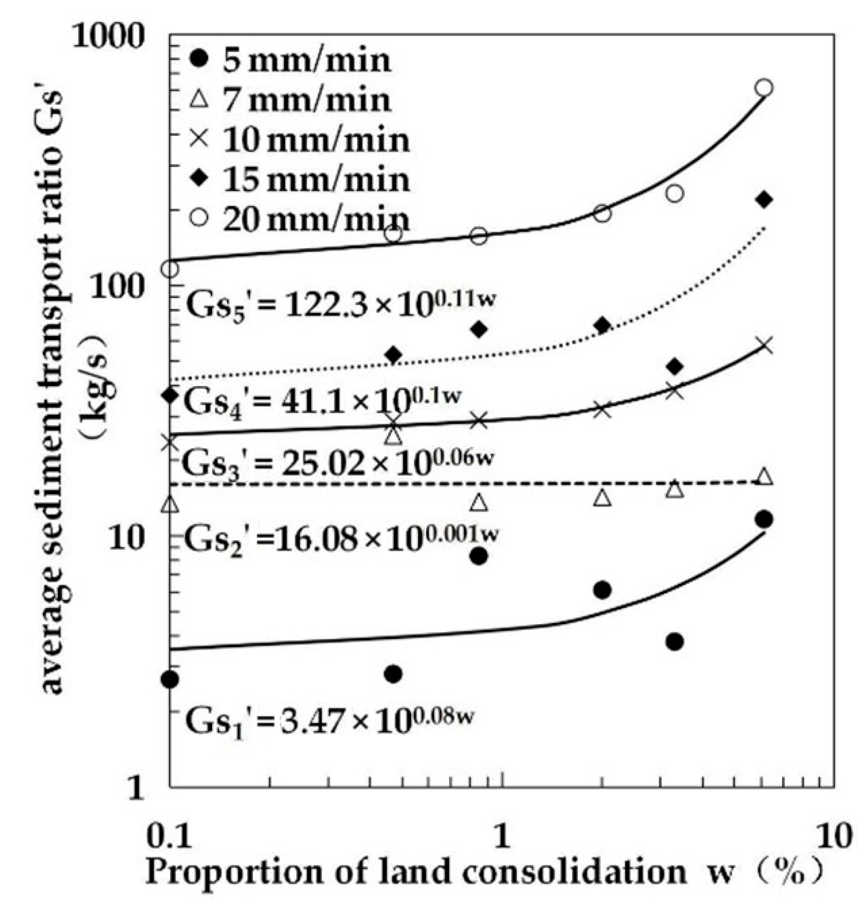
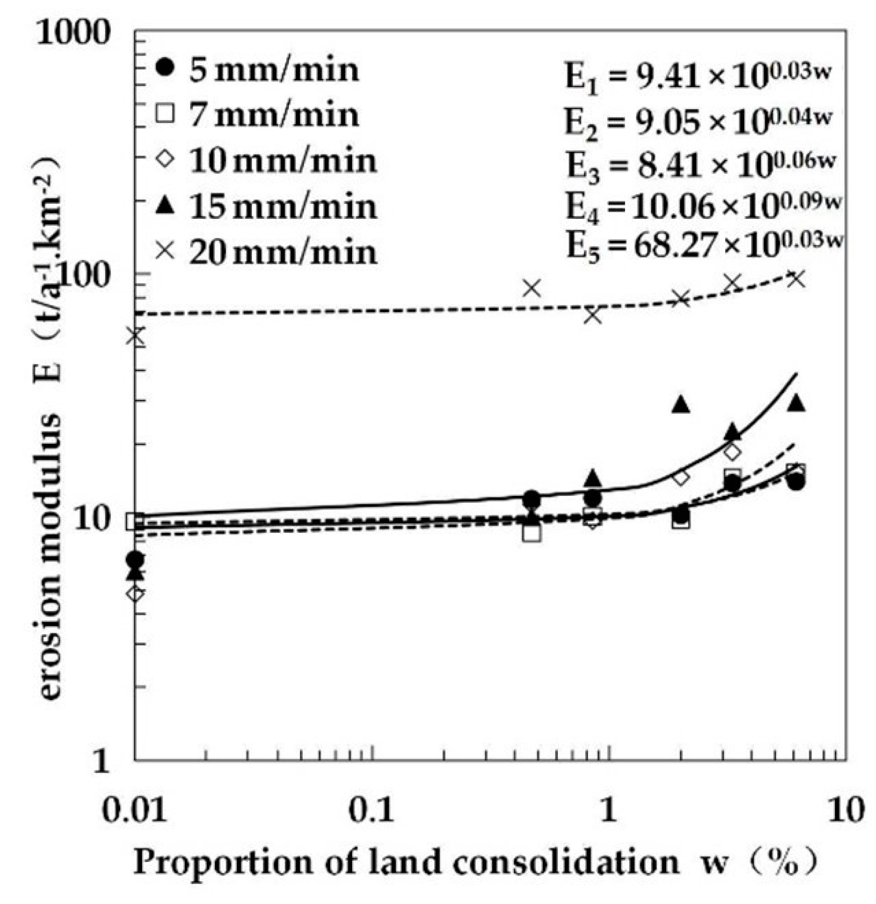
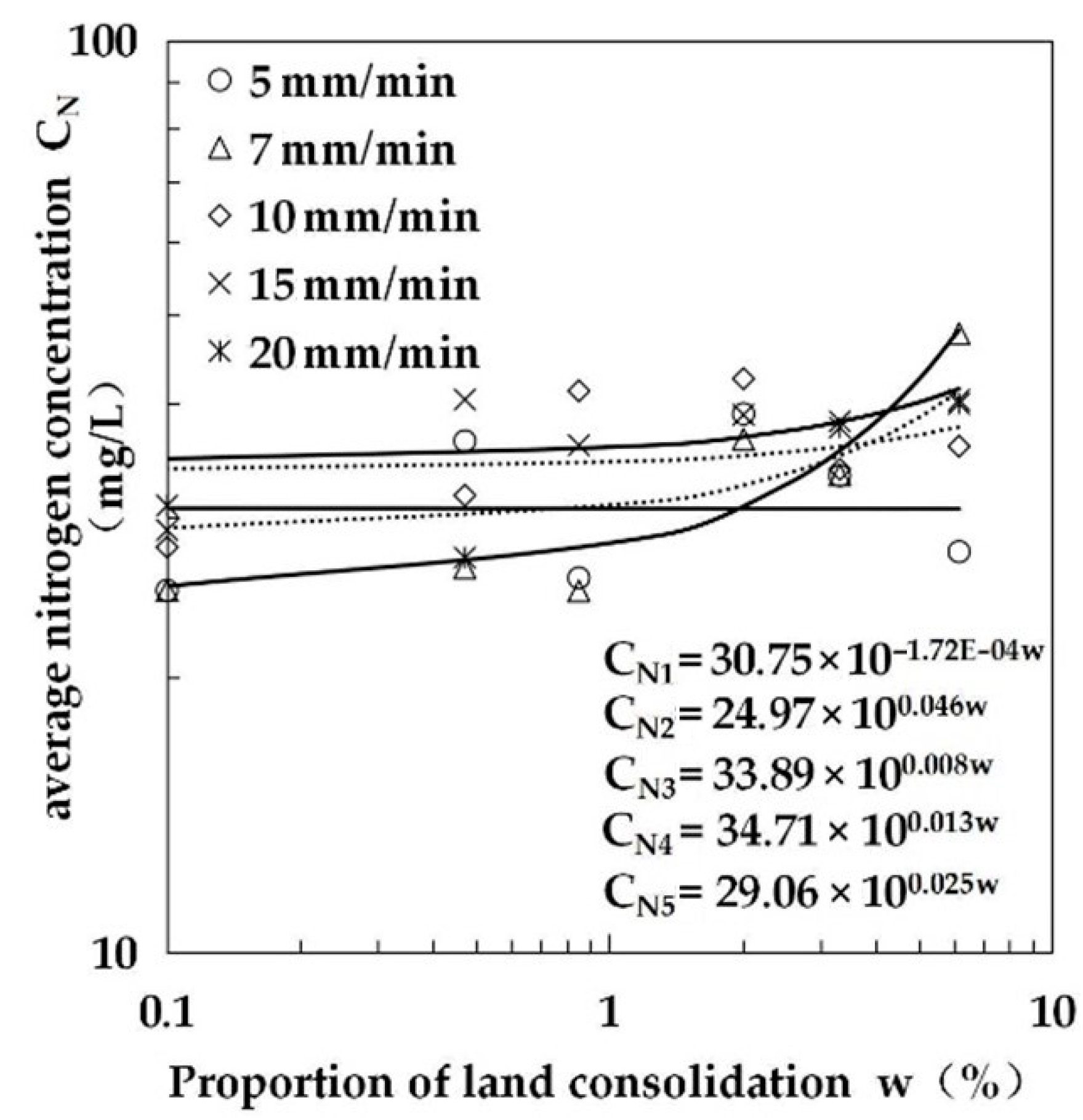
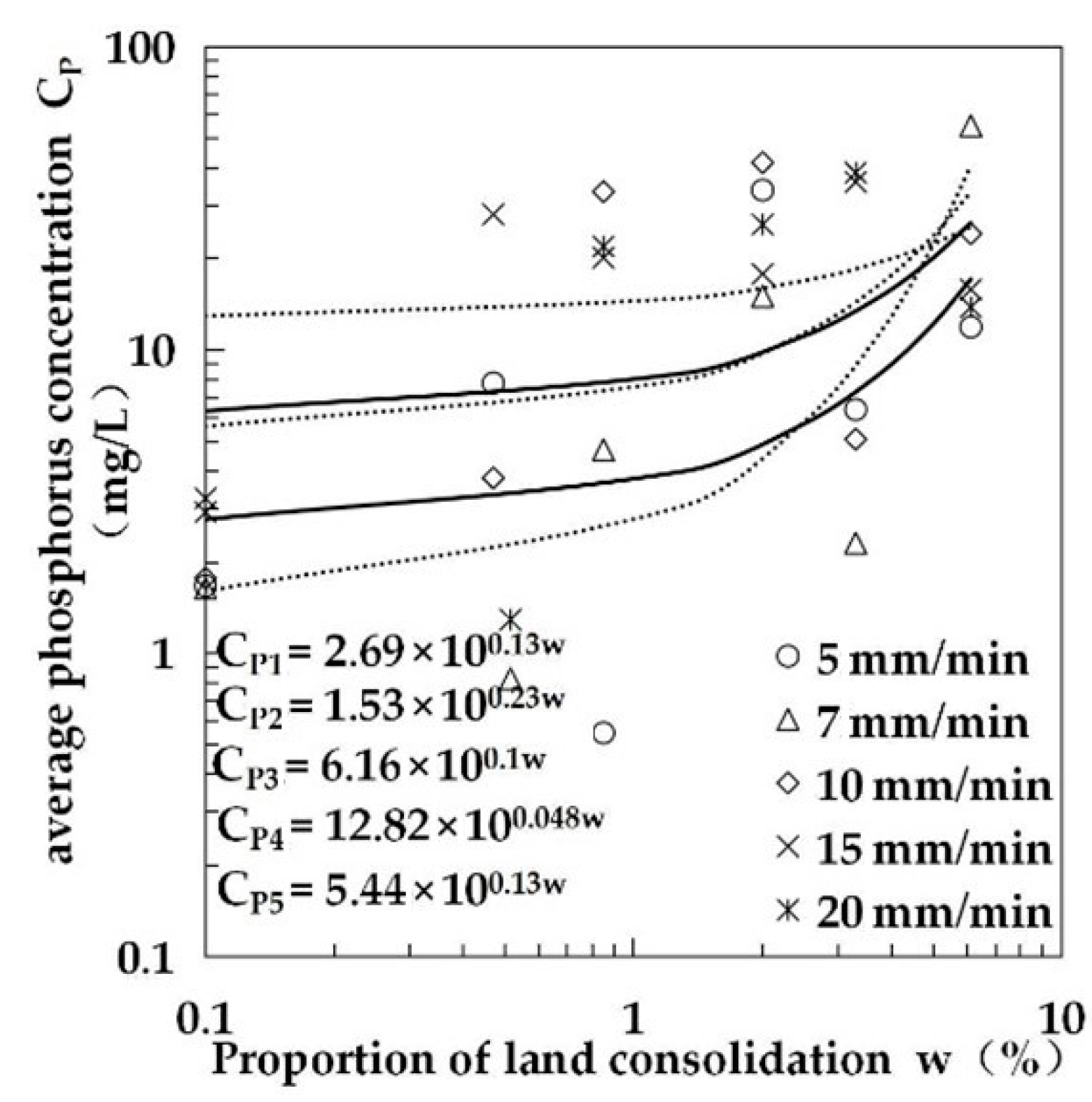
3.3.2. The Impact on Pollutant Transport

Figure 29 and Figure 30 show the changes in average nitrogen and phosphorus concentrations at the outlet for a given land consolidation proportion, under different rainfall intensities. These figures show that the average concentrations of nitrogen and phosphorus at the outlet of the watershed increased with increasing land consolidation proportion under different rain intensities. The greater the rainfall intensity, the higher the land consolidation proportion with more pollutant concentrations. The relationships can be represented by the following exponential functions:

$$C_N = 30.7\times {10}^{0.023w}$$

(16)

$$C_P = 5.73\times {10}^{0.13w}$$

(17)

As shown in the figures, the curves were almost horizontal in the land consolidation proportion ranging from 0–2%; however, the varying degrees of land consolidation projects increased the pollutant output concentration of the watershed. When balancing the relationship between the efficient use of land resources in the watershed and the control of pollutant output risk, it is recommended that the consolidation proportion remains below 2%.

As a result of the above analyses, it was possible to identify the functional relationships between the erosional transport parameters, land consolidation proportion (w), and rainfall intensities (i) in HMSW in the LHGR; the recommended consolidation proportions are presented in

Table 5. Changes in the small watershed erosion and transport parameters and the recommended consolidation proportion.

Runoff Sediment Parameter	Law of Change	Proposed Consolidation Proportion
Runoff generation time (tc)	$t_c = 95.3\times {10}^{0.08w-0.04i}$	≤3.3%
Flood peak time (th)	$t_h = 386\times {10}^{0.06w-0.03i}$	≤2%
Flood peak discharge (Qh)	$Q_h = \{\begin{array}{c}2.85\times {10}^{-0.03w}\left(i\le 5 mm/min\right)\\ 2.39\times {10}^{0.03w+0.06i}(i>5 mm/min)\end{array}$	≤3.3%
Average outlet discharge (Qp)	$Q_p = \{\begin{array}{c}2.25\times {10}^{-0.02w}\left(i\le 5 mm/min\right)\\ 1.76\times {10}^{0.02w+0.06i}(i>5 mm/min)\end{array}$	≤3.3%
Peak sediment discharge time (ts)	$t_s = \{\begin{array}{c}212.8\times {10}^{0.08w-0.02i}\left(i\le 7 mm/min\right)\\ 334.7\times {10}^{-\left(0.05w+0.03i\right)}(i>5 mm/min)\end{array}$	≤3.3%
Peak sediment discharge value (Sf)	$S_f = 1.44\times {10}^{0.08w+0.02i}$	≤3.3%
Average sediment content atoutlet (Sp)	$S_p = 1.31\times {10}^{0.07w+0.02i}$	≤3.3%
Average sediment transport ratio at outlet (Gs′)	$G_{s\prime } = 2.36\times {10}^{0.09\left(w+i\right)}$	≤3.3%
Soil erosion modulus (E)	$E = 3.58\times {10}^{0.05\left(i+w\right)}$	≤3.3%
Average nitrogen concentration at outlet (CN)	$C_N = 30.7\times {10}^{0.023w}$	≤2%
Average phosphorusconcentration at outlet (CP)	$C_P = 5.73\times {10}^{0.13w}$	≤2%

. The above results can be used as a reference for the calculation of runoff generation, collection and the design of land consolidation of small watersheds under high management in the Loess Plateau of China or other parts of the world.

4. Discussion

4.1. Physical Scale Model Simulation

GLCP in the LHGR is typically based on small watersheds [38] with a series and parallel styles. The conditions in small watersheds are usually complex and have a substantial impact on the evolution of the erosional environment; therefore, the layout requires optimization. However, the topography of a small watershed is highly complex, showing strong three-dimensionality, and the mathematical model employed in the small watershed simulation process has to be generalized and simplified, which makes calculation accuracy difficult to guarantee [39,40,41]. In most cases, the issues can only be described qualitatively [42,43]. It remains difficult to accurately reconstruct the scene [44,45,46]. Therefore, determining the impact of a land consolidation project on the evolution of the erosional environment remains an important issue in gully land consolidation.

In this study, a physical scale simulation technology was introduced. This method was strongly three-dimensional in promoting runoff, sediment, and pollutant transportation. This method was also able to reproduce the evolution and developmental processes of the watershed erosional environment under different rainfall amounts, vegetation coverage levels, and consolidation conditions, which allowed analysis of the impact of engineering measures on the hydrological processes in the watershed; such information is useful for optimizing the project layout [47,48,49]. The experiment in the present study focused on the evolution of the erosional environment of small watersheds before and after management and the variability of the watershed’s erosional transport conditions under different land consolidation proportions. The results showed that runoff and sediment generation were clearly suppressed after vegetation restoration and that the effects on soil and water conservation were more obvious after vegetation restoration than before. A critical value in the scale of the GLCP in the highly managed watershed was identified; however, within a certain range, the land consolidation activities increased the erosion base level and reduced and delayed floods and the transport of sediment and pollutants. The results showed that this method has broad developmental prospects for studying the impacts of various projects on the evolution of the erosional environment in watersheds.

4.2. The Determination of Pollutant Scale

Nonpoint source pollutant results from GLCP include rainfall erosion and pollutant transport. The hydrodynamic erosion mechanism in this study was so complex that it was difficult to provide equations and scales for N, P, K, and pesticides theoretically, and there was little literature available for reference [50,51,52,53,54]. Drawing on the experience of determining the sediment carrying capacity scale in river engineering model tests [55], the authors adopted the ratio of the pollutant content in the corresponding plots between the model and prototype as the test scale. The theoretical basis was the similarity theory. It was determined that similarity in the boundary conditions is a sufficient and necessary condition to ensure the similarity of the model and prototype and that similar models and prototypes obey the same physical equation. Through experimental verification, this method was determined to be reasonable. This method expands the mechanisms for experimental research and is of great significance for simulating complex erosional environments.

4.3. Increasing Erosion and Changes in Runoff Generation-Collection Mechanisms in Highly Managed Watersheds under Extreme Rainstorm Conditions

With climate change, extreme rainstorms are expected to increase in frequency on the Loess Plateau [56,57]. Extreme rainstorms increase erosion rates in highly managed watersheds, and this has been consistently found at home and abroad [58,59,60,61]. Accordingly, in this study, erosion increased significantly under high rain intensities as the vegetation coverage reached 0.9. Therefore, critical values for the land scale should be considered based on different vegetation coverage levels and rain intensities for HMSW.

Another issue requiring attention is the changing runoff generation–convergence mechanism in highly managed watersheds [62]. This experiment found that the flood discharge peaks are delayed compared to the sediment discharge peaks under high-level management. This finding is inconsistent with previous understanding of the characteristics of generation and collection in the Loess Plateau. Whether the significant improvement in vegetation indicates changes in runoff generation and collection mechanisms requires careful study.

5. Conclusions

Based on the above discussion, the following conclusions were drawn:

A new method for determining the scale of pollutants was developed, which can be applied under similar boundary conditions to meet the similarity requirements for rainfall, runoff, erosion, sediment transport, and deformation of bed surfaces. This method considered the average ratio of pollutant content at corresponding typical areas of the prototype and model. In this experiment, the nitrogen and phosphorus contents of corresponding typical areas in the prototype and model were surveyed and sampled and scale curves were generated along different positions in the prototype and model. From the results, when the geometric scale was ${\lambda }_l = 100$, the nitrogen and phosphorus content scales of the erosion nonpoint source pollutants were determined to be ${\lambda }_{Nm} = 0.5$ and ${\lambda }_{Pm} = 0.9$. This finding was verified by the designed similarity simulation test. By using this technique, a perfect similarity criterion and method for simulating the evolution of the erosion environment in small watersheds were established.

After the vegetation coverage reached 90%, the runoff generation, flood peak appearance time, and sediment peak appearance time were increased by a factor of 3.1, and the flood peak discharge and sediment peak discharge values were reduced by over 93%. Another finding was that the current flood peak lagged behind the sediment peak. This finding suggests that a significant change in the runoff production mechanisms might have occurred.

In highly managed watersheds, the degree of impact on the erosional environment varied with the proportion of consolidated land. The quantitative relationships among the erosion dynamic parameters, land consolidation proportion, and rainfall intensity were identified. The critical values of consolidation proportion were recommended as 0.85% and 3.3%—when it exceeded 0.85%, there was a certain degree of impact, when it exceeded 3.3%, the impact was more obvious. This study provides a reference for the design, planning, and implementation of land consolidation projects on the Loess Plateau and other parts of the world.

References

1. Chen, L.; Yang, L.; Wei, W.; Wang, Z.; Mo, B.; Cai, G. Towards Sustainable Integrated Watershed Ecosystem Management: A Case Study in Dingxi on the Loess Plateau, China. Environ. Manag. 2013, 51, 126–137. [Google Scholar] [CrossRef] [PubMed]
2. Godfray, H.C.J.; Beddington, J.R.; Crute, I.R.; Haddad, L.; Lawrence, D.; Muir, J.F.; Pretty, J.; Robinson, S.; Thomas, S.M.; Toulmin, C. Food security: The challenge of feeding 9 billion people. Science 2010, 327, 812–818. [Google Scholar] [CrossRef] [PubMed] [Green Version]
3. Li, P.Y.; Qian, H.; Wu, J.H. Environment: Accelerate research on land creation. Nature 2014, 510, 29–31. [Google Scholar] [CrossRef] [PubMed]
4. Deng, L.; Kim, D.G.; Li, M.Y.; Huang, C.B.; Liu, Q.Y.; Cheng, M.; Shangguan, Z.P.; Peng, C.H. Land-use changes driven by ‘Grain for Green’ program reduced carbon loss induced by soil erosion on the Loess Plateau of China. Glob. Planet. Chang. 2019, 177, 101–115. [Google Scholar] [CrossRef]
5. Li, P.Y.; Chen, Y.J.; Hu, W.H.; Li, X.; Yu, Z.R.; Liu, Y.H. Possibilities and requirements for introducing agri-environment measures in land consolidation projects in China, evidence from ecosystem services and farmers’ attitudes. Sci. Total Environ. 2019, 650, 3145–3155. [Google Scholar] [CrossRef]
6. Li, Y.R.; Li, Y.; Fan, P.C.; Long, H.L. Impacts of land consolidation on rural human-environment system in typical watershed of the Loess Plateau and implications for rural development policy. Land Use Policy 2019, 86, 339–350. [Google Scholar]
7. Jin, Z.; Guo, L.; Wang, Y.Q.; Yu, Y.L.; Lin, H.; Chen, Y.P.; Chu, G.C.; Zhang, J.; Zhang, N.P. Valley reshaping and damming induce water table rise and soil salinization on the Chinese Loess Plateau. Geoderma 2019, 339, 115–125. [Google Scholar] [CrossRef]
8. He, C.X. The situation, characteristics and effect of the gully reclamation project in Yan’an. Environ. Earth Sci. 2015, 6, 255–260, (In Chinese with English abstract). [Google Scholar]
9. Jin, Z. The creation of farmland by gully filling on the Loess Plateau: A double-edged sword. Environ. Sci. Technol. 2014, 48, 883–884. [Google Scholar] [CrossRef] [PubMed]
10. Liu, Q.; Wang, Y.Q.; Zhang, J.; Chen, Y.P. Filling gullies to create farmland on the Loess Plateau. Environ. Sci. Technol. 2013, 47, 7589–7590. [Google Scholar] [CrossRef]
11. Liu, Y.S.; Li, Y.H. Environment: China’s land creation project stands firm. Nature 2014, 511, 410. [Google Scholar] [CrossRef]
12. Liu, Y.S.; Guo, Y.J.; Li, Y.R.; Li, Y.H. GIS-based effect assessment of soil erosion before and after gully land consolidation: A case study of Wangjiagou project region, Loess Plateau. Chin. J. Geogr. Sci. 2015, 25, 137–146. [Google Scholar] [CrossRef] [Green Version]
13. Liu, Y.S.; Li, Y.R. Engineering philosophy and design scheme of gully land consolidation in Loess Plateau. Trans. Chin. Soc. Agric. Eng. 2017, 10, 1–9. [Google Scholar]
14. Munnangi, A.K.; Lohani, B.; Misra, S.C. A review of land consolidation in the state of Uttar Pradesh, India: Qualitative approach. Land Use Policy 2020, 90, 104309. [Google Scholar] [CrossRef]
15. Hiironen, J.; Riekkinen, K. Agricultural impacts and profitability of land consolidations. Land Use Policy 2016, 55, 309–317. [Google Scholar] [CrossRef]
16. Guo, Y.; Liu, Y.; Wen, Q.; Li, Y. The Transformation of agricultural development towards a sustainable future from an evolutionary view on the Chinese Loess Plateau: A Case Study of Fuxian County. Sustainability 2014, 6, 3644–3668. [Google Scholar] [CrossRef] [Green Version]
17. Liu, G.; Hu, F.N.; Abd Elbasit, M.A.M.; Zheng, F.L.; Liu, P.L.; Xiao, H.; Zhang, Q.; Zhang, J.Q. Holocene erosion triggered by climate change in the central Loess Plateau of China. Catena 2018, 160, 103–111. [Google Scholar] [CrossRef]
18. Lei, N.; Mu, X.M. Analysis on effect of gully control and land reclamation projects on carbon emission in hilly and gully regions of Loess Plateau. J. Agro-Environ. Sci. 2018, 2, 392–398. [Google Scholar]
19. Chen, Y.P.; Wu, J.H.; Wang, H.; Ma, J.F.; Su, C.C.; Wang, K.B.; Wang, Y. Evaluating the soil quality of newly created farmland in the hilly and gully region on the Loess Plateau, China. J. Geogr. Sci. 2019, 5, 791–802. [Google Scholar] [CrossRef] [Green Version]
20. Chen, Y.P.; Zhang, Y. Sustainable Model of Rural Vitalization in Hilly and Gully Region on Loess Plateau. Bull. Chin. Acad. Sci. 2019, 6, 708–716. [Google Scholar]
21. Wei, O.Y.; Hao, F.H.; Skidmore, A.K.; Toxopeus, A.G. Soil erosion and sediment yield and their relationships with vegetation cover in upper stream of the Yellow River. Sci. Total Environ. 2010, 409, 396–403. [Google Scholar]
22. Zhang, X.B.; Jin, Z. Gully land consolidation project in Yan’an is inheritance and development of wrap land dam project on the Loess Plateau. J. Earth Environ. 2015, 4, 261–264. [Google Scholar]
23. Zhang, X.B.; Vries, W.T.; Li, G.; Ye, Y.M.; Zheng, H.Y.; Wang, M.R. A behavioral analysis of farmers during land reallocation processes of land consolidation in China: Insights from Guangxi and Shandong provinces. Land Use Policy 2019, 89, 104230. [Google Scholar] [CrossRef]
24. Li, W.J.; Gao, X.; Wang, R.; Du, L.L.; Hou, F.B.; He, Y.; Hu, Y.X.; Yao, L.G.; Guo, S.L. Soil redistribution reduces integrated C sequestration in soil-plant ecosystems: Evidence from a five-year topsoil removal and addition experiment. Geoderma 2020, 377, 114593. [Google Scholar] [CrossRef]
25. Sun, P.C.; Wu, Y.P.; Yang, Z.F.; Sivakumar, B.; Qiu, L.J.; Liu, S.G.; Cai, Y.P. Can the Grain-for-Green program really ensure a low sediment load on the chinese Loess Plateau? Engineering 2019, 5, 855–864. [Google Scholar] [CrossRef]
26. Jiang, G.H.; Wang, X.P.; Yun, W.J.; Zhang, R.J. A new system will lead to an optimal path of land consolidation spatial management in China. Land Use Policy 2015, 42, 27–37. [Google Scholar]
27. Jiang, G.H.; Zhang, R.J.; Ma, W.Q.; Zhou, D.Y.; Wang, X.P.; He, X. Cultivated land productivity potential improvement in land consolidation schemes in Shenyang, China: Assessment and policy implications. Land Use Policy 2017, 68, 80–88. [Google Scholar] [CrossRef]
28. Lou, X.Y.; Gao, J.E.; Han, S.Q.; Guo, Z.H.; Yin, Y. Influence of land consolidation engineering of gully channel on watershed runoff yield and concentration in Loess Hilly and Gully Region. Water Resour. Power 2016, 10, 23–27. [Google Scholar]
29. Sun, P.C.; Gao, J.E.; Han, S.Q.; Yin, Y.; Zhou, M.F.; Han, J.Q. Simulation study on the effects of typical gully land consolidation on runoff-sediment-nitrogen emissions in the loess hilly-gully region. J. Agro-Environ. Sci. 2017, 6, 1177–1185. [Google Scholar]
30. Kang, Y.C.; Gao, J.E.; Shao, H.; Zhang, Y.Y. Quantitative analysis of hydrological responses to climate variability and land-use change in the hilly-gully region of the Loess Plateau, China. Water 2020, 12, 82. [Google Scholar] [CrossRef] [Green Version]
31. Dou, S.H.; Gao, J.E.; Li, X.H.; Gao, Z.; Liu, S.X.; Zhou, F.F. Drainage design of channel land consolidation project in gully areas of Loess Hilly Region. Bull. Soil Water Conserv. 2020, 3, 310–316. [Google Scholar]
32. Janus, J.; Markuszewska, I. Land consolidation—A great need to improve effectiveness. A casestudy from Poland. Land Use Policy 2017, 65, 143–153. [Google Scholar] [CrossRef]
33. Janus, J.; Markuszewska, I. Forty years later: Assessment of the long-lasting effectiveness of land consolidation projects. Land Use Policy 2019, 83, 22–31. [Google Scholar] [CrossRef]
34. Guo, B.B.; Fang, Y.L.; Jin, X.B.; Zhou, Y.K. Monitoring the effects of land consolidation on the ecological environmental quality based on remote sensing: A case study of Chaohu Lake Basin, China. Land Use Policy 2020, 95, 104569. [Google Scholar] [CrossRef]
35. Zhang, Z.F.; Zhao, W.; Gu, X.K. Changes resulting from a land consolidation project (LCP) and its resource-environment effects: A case study in Tianmen City of Hubei Province, China. Land Use Policy 2014, 40, 74–82. [Google Scholar] [CrossRef]
36. Gao, J.E.; Wu, P.T.; Niu, W.Q.; Feng, H.; Fan, H.H.; Yang, S.W. Simulation experiment design and verification of controlling water erosion on small watershed of loess plateau. Trans. Chin. Soc. Agric. Eng. 2005, 10, 41–45. [Google Scholar]
37. Gao, J.E.; Yang, S.W.; Wu, P.T.; Wang, G.Z.; Shu, R.J. Preliminary study on similitude law in simulative experiment for controlling hydraulic erosion. Trans. Chin. Soc. Agric. Eng. 2006, 1, 27–31. [Google Scholar]
38. Yuan, J.P.; Lei, T.W.; Jiang, D.S.; Zhou, Q.Y. Simulated experimental study on normalized integrated model for different degrees of erosion control for small watersheds. Trans. Chin. Soc. Agric. Eng. 2000, 1, 22–25. [Google Scholar]
39. Mu, X.M.; Li, P.F.; Gao, P.; Zhao, G.J.; Sun, W.Y. Review and evaluation of soil erosion models applied to China Loess Plateau. Yellow River 2016, 38, 100–114. [Google Scholar]
40. Momm, H.G.; Bingner, R.L.; Wells, R.R.; Porter, W.S.; Yasarer, L.; Dabney, S.M. Enhanced field-scale characterization for watershed erosion assessments. Environ. Model. Softw. 2019, 117, 134–148. [Google Scholar] [CrossRef]
41. Zheng, F.L.; Zhang, X.C.; Wang, J.X.; Flanagan, D.C. Assessing applicability of the WEPP hillslope model to steep landscapes in the northern Loess Plateau of China. Soil Tillage Res. 2020, 197, 104492. [Google Scholar] [CrossRef]
42. Zhang, G.H. Research situation and prospect of the soil erosion model. Adv. Water Sci. 2002, 3, 389–396. [Google Scholar]
43. Zhang, G.H. Several ideas related to soil erosion research. J. Soil Water Conserv. 2020, 4, 21–30. [Google Scholar]
44. Hessel, R. Consequences of hyper concentrated flow for process-based soil erosion modelling on the Chinese Loess Plateau. Earth Surf. Process. Landf. 2006, 31, 1100–1114. [Google Scholar] [CrossRef]
45. Furl, C.; Sharif, H.; Jeong, J. Analysis and simulation of large erosion events at central Texas unit source watersheds. J. Hydrol. 2015, 527, 494–504. [Google Scholar] [CrossRef]
46. Heilig, A.; DeBruyn, D.; Walter, M.T. Testing of a mechanistic soil erosion model with a simple experiment. J. Hydrol. 2001, 244, 9–16. [Google Scholar] [CrossRef] [Green Version]
47. Li, S.Q.; Gao, J.E.; Shao, H.; Zhao, C.H.; Yang, S.W.; Liang, G.G. Effects of model material selection on the similarity of erosion processes in hydraulic erosion simulation experiment. J. Soil Water Conserv. 2009, 23, 6–10. [Google Scholar]
48. Li, S.Q.; Gao, J.E.; Zhao, C.H.; Shao, H.; Liang, G.G. Design and verification of water erosion scale simulation experiment on slop. Sci. Soil Water Conserv. 2010, 8, 6–12. [Google Scholar]
49. Yin, Y.; Gao, J.E.; Li, H.J.; Han, S.Q.; Zhou, M.F. Study on extraction methods for hydrodynamic parameters of overland sediment flow. J. Soil Water Conserv. 2019, 33, 25–38. [Google Scholar]
50. Yang, S.Q. Sediment transport capacity in rivers. J. Hydraul. Res. 2005, 2, 131–138. [Google Scholar] [CrossRef]
51. Yang, S.Q.; Koh, S.C.; Kim, I.S.; Song, Y.C. Sediment transport capacity-An improved Bagnold formula. Int. J. Sediment Res. 2007, 1, 27–38. [Google Scholar]
52. Milhous, R.T. Climate change and changes in sediment transport capacity in the Colorado Plateau, USA. Sediment Budg. 2005, 2, 271–278. [Google Scholar]
53. Zhang, Y.B.; Zheng, F.L.; Wu, M. Research progresses in agricultural non-point source pollution caused by soil erosion. Adv. Water Sci. 2007, 1, 123–132. [Google Scholar]
54. Zhao, Q.; Wang, K.; Huang, J.S.; Dong, J.W. Migration rule of non-point source pollutions from seasonal frozen soil in small watershed scale during thawing period. Trans. Chin. Soc. Agric. Eng. 2015, 1, 139–145. [Google Scholar]
55. Wang, M.J.; Luo, L.; Lu, H.W.; Jiang, H. Similarity law of water pollutant biodegradation in model experiment. J. Sichuan Univ. (Eng. Sci. Ed.) 2004, 2, 25–28. [Google Scholar]
56. Li, Z.B.; Zhu, B.B.; Li, P. Advancement in study on soil erosion and soil and water conservation. Acta Pedol. Sin. 2008, 45, 803–809. [Google Scholar]
57. Yuan, X.B.; Shang, Z.Y.; Niu, D.C.; Fu, H. Advances in ecological degeneration and restoration of Loess Plateau. Pratacultural Sci. 2015, 32, 363–371. [Google Scholar]
58. Liang, W.; Fu, B.J.; Wang, S.; Zhang, W.B.; Jin, Z.; Feng, X.M.; Yan, J.W.; Liu, Y.; Zhou, S. Quantification of the ecosystem carrying capacity on China’s Loess Plateau. Ecol. Indic. 2019, 101, 192–202. [Google Scholar] [CrossRef]
59. Xiao, H.; Liu, G.; Liu, P.L.; Zheng, F.L.; Zhang, J.Q.; Hu, F.N. Sediment transport capacity of concentrated flows on steep loessial slope with erodible beds. Sci. Rep. 2017, 7, 2350. [Google Scholar] [CrossRef]
60. Xiao, H.; Liu, G.; Zhang, Q.; Zheng, F.L.; Zhang, X.C.; Liu, P.L.; Zhang, J.Q.; Hu, F.N.; Abd-Elbasit, M.A.M. Quantifying contributions of slaking and mechanical breakdown of soil aggregates to splash erosion for different soils from the Loess Plateau of China. Soil Tillage Res. 2018, 178, 150–158. [Google Scholar] [CrossRef]
61. Liu, G.; Tian, F.X.; Warrington, D.N.; Zheng, S.Q.; Zhang, Q. Efficacy of grass for mitigating runoff and erosion from an artificial loessial earthen road. Trans. Asabe 2010, 53, 119–125. [Google Scholar] [CrossRef]
62. Coelho, A.T.; Galvão, T.C.B.; Pereira, A.R. The effects of vegetative cover in the erosion prevention of a road slope. Environ. Manag. Health 2001, 12, 78–87. [Google Scholar] [CrossRef]
Figure 1. Location and different stages of the Kangjiagelao watershed, (a) Location and early status of the Kangjiagelao watershed, (b) Current status of the Kangjiagelao watershed.
Water 13 01540 g001
Figure 2. The sediment particle grading curves of the model and prototype.
Water 13 01540 g002
Figure 3. The model built according to the two situations, (a) No vegetation restoration, (b) High-level vegetation restoration.
Water 13 01540 g003
Figure 4. Model water supply and rainfall equipment.
Water 13 01540 g004
Figure 5. Different scales of land consolidation projects.
Water 13 01540 g005
Figure 6. Gully land consolidation profile ( λ l   =   100 ).
Water 13 01540 g006
Figure 7. Water sample collection and detection.
Water 13 01540 g007
Figure 8. Total nitrogen content at each sampling point for the prototype and model of the small watershed.
Water 13 01540 g008
Figure 9. Fixed scale of pollutant nitrogen rate at different sampling points.
Water 13 01540 g009
Figure 10. Total phosphorus content at each sampling point for the prototype and model of the small watershed.
Water 13 01540 g010
Figure 11. Fixed scale of pollutant phosphorus rate at different sampling points.
Water 13 01540 g011
Figure 12. Changes in soil nitrogen content with distance in trenches of the prototype and model.
Water 13 01540 g012
Figure 13. Changes in soil phosphorus content with distance in trenches of the prototype and model.
Water 13 01540 g013
Figure 14. Changes in runoff generation time with rain intensity before and after vegetation restoration.
Water 13 01540 g014
Figure 15. Changes in peak flood discharge value with rain intensity before and after vegetation restoration.
Water 13 01540 g015
Figure 16. Changes in peak sediment discharge time with rain intensity before and after control.
Water 13 01540 g016
Figure 17. Changes in erosion modulus with rain intensity before and after control.
Water 13 01540 g017
Figure 18. Changes in flow and sediment content before watershed control.
Water 13 01540 g018
Figure 19. Changes in flow and sediment content after high-level watershed control.
Water 13 01540 g019
Figure 20. Changes in flow and sediment content after high-level watershed control.
Water 13 01540 g020
Figure 21. Changes in peak flood discharge time with the proportion of land consolidation under different rainfall intensities.
Water 13 01540 g021
Figure 22. Changes in peak flood discharge value with land consolidation proportion under different rainfall intensities.
Water 13 01540 g022
Figure 23. Changes in average outlet discharge with land consolidation proportion under different rainfall intensities.
Water 13 01540 g023
Figure 24. Changes in peak sediment discharge time with land consolidation proportion under different rainfall intensities.
Water 13 01540 g024
Figure 25. Changes in peak sediment discharge value with land consolidation proportion under different rainfall intensities.
Water 13 01540 g025
Figure 26. Changes in average sediment content at the outlet section with land consolidation proportion under different rain intensities.
Water 13 01540 g026
Figure 27. Changes in the average sediment transport ratio with land consolidation proportion under different rain intensities.
Water 13 01540 g027
Figure 28. Changes in erosion modulus with land consolidation proportion under a rainfall capacity of 150 mm.
Water 13 01540 g028
Figure 29. Changes in average nitrogen concentration at the outlet with land consolidation proportion under different rainfall intensities.
Water 13 01540 g029
Figure 30. Changes in average phosphorus concentration at the outlet with land consolidation proportion under different rainfall intensities.
Water 13 01540 g030