
Application of SWAT in Hydrological Simulation of Complex Mountainous River Basin (Part I: Model Development)

1
Central Department of Hydrology and Meteorology, Tribhuvan University, Kathmandu 44600, Nepal
2
Nepal Academy of Science and Technology (NAST), Kathmandu 44600, Nepal
3
Water Modeling Solutions Pvt. Ltd. (WMS), Kathmandu 44600, Nepal
*
Author to whom correspondence should be addressed.
Water 2021, 13(11), 1546; https://doi.org/10.3390/w13111546
Submission received: 8 April 2021
/
Revised: 23 May 2021
/
Accepted: 24 May 2021
/
Published: 31 May 2021
Abstract
:The soil and water assessment tool (SWAT) hydrological model has been used extensively by the scientific community to simulate varying hydro-climatic conditions and geo-physical environment. This study used SWAT to characterize the rainfall-runoff behaviour of a complex mountainous basin, the Budhigandaki River Basin (BRB), in central Nepal. The specific objectives of this research were to: (i) assess the applicability of SWAT model in data scarce and complex mountainous river basin using well-established performance indicators; and (ii) generate spatially distributed flows and evaluate the water balance at the sub-basin level. The BRB was discretised into 16 sub-basins and 344 hydrological response units (HRUs) and calibration and validation was carried out at Arughat using daily flow data of 20 years and 10 years, respectively. Moreover, this study carried out additional validation at three supplementary points at which the study team collected primary river flow data. Four statistical indicators: Nash–Sutcliffe efficiency (NSE), percent bias (PBIAS), ratio of the root mean square error to the standard deviation of measured data (RSR) and Kling Gupta efficiency (KGE) have been used for the model evaluation. Calibration and validation results rank the model performance as “very good”. This study estimated the mean annual flow at BRB outlet to be 240 m3/s and annual precipitation 1528 mm with distinct seasonal variability. Snowmelt contributes 20% of the total flow at the basin outlet during the pre-monsoon and 8% in the post monsoon period. The 90%, 40% and 10% exceedance flows were calculated to be 39, 126 and 453 m3/s respectively. This study provides additional evidence to the SWAT diaspora of its applicability to simulate the rainfall-runoff characteristics of such a complex mountainous catchment. The findings will be useful for hydrologists and planners in general to utilize the available water rationally in the times to come and particularly, to harness the hydroelectric potential of the basin.
1. Introduction
Complex interactions between the atmospheric system and the underlying topography determine river discharge. It is a part of rainfall that appears in a stream and represents the total response of a basin. Surface flow, subsurface flow, base flow and precipitation that directly falls on the stream constitutes the total discharge in the river [1,2]. Time series of flow data is one of the most important requirements for planning, operation and control of all water resources projects [3,4,5]. However, measured flow data are not available in most of the cases in such project sites [5]. It is because of the lack of sufficient flow gauging stations in most river basins. The situation is more severe in mountainous basins [6] because of the inaccessibility of most of these sites for local observations. It is the reason why water budget analyses in such basins are not as easy as in other gauged basins [7,8]. However, most of the large rivers (e.g., the Ganga, the Indus, the Sutlej, the Brahmaputra, the Mekong, the Yellow) in the world originate from the mountains and are perennial in nature as they are constantly fed by snow and glaciers. Mountain basins might have, thus, been considered as the water towers of the world [7,9].
The characteristics of the river basins are usually controlled by the geo-physical environment and hydro-climatic conditions [10]. In central Himalaya, high relief with steep topography along with tectonic activities, climate-driven erosional process and high sediment yield, among many other factors, make the basins complex [11]. Precipitation in Nepalese mountainous river basins, including the Budhigandaki River Basin (BRB), are mostly influenced by orography, aspect and physiography, with more amount of precipitation in the windward side than in leeward side [12,13,14,15,16,17,18]. The challenge is further exacerbated due to limited data availability in these regions because of difficult access.
To address the challenge of non-availability of observed data at local level for water resources planning and utilization in the river basin, hydrologic simulation method has been widely used in recent years [19,20,21,22,23]. Simulation models provide excellent platforms for evaluating various options for water resources as well as environmental planning [24,25]. In hydrological simulation, a hydrologic model which is a simplified software representation of the hydrological process within a basin boundary, is used to generate the flow at required locations of the river basin.
Based on spatial discretization, three types of model are in practice: lumped, semi-distributed and fully-distributed. For example, Hydrologiska Byråns Vattenbalansavdelning (HBV), GR4J (Génie Rural à four paramètres Journalier), hydrological model (HYMOD), artificial neural network (ANN) based data-driven hydrological models, simplified version of the HYDROLOG (SIMHYD), Snowmelt Runoff Model (SRM) and TANK are lumped models while the Soil and Water Assessment Tool (SWAT), topographic hydrologic model (TOPMODEL), Variable Infiltration Capacity (VIC) and Hydrologic Engineering Center—Hydrologic Modeling System (HEC-HMS), are semi distributed ones. Variant of Système Hydrologique Européen (MIKE SHE) and Visualizing Ecosystem Land Management Assessments (VELMA) are fully distributed models [25,26,27,28]. These are either event-based (e.g., Runoff Analysis and Fow Training, RAFT) or continuous (e.g., MIKE SHE, SWAT) flow generating models [29,30].
The SWAT model [30,31] has been chosen among many hydrological models for this study. Several studies have been carried out to assess the water availability and impacts of climate change; land use and land cover changes around the world using SWAT model [21,32,33,34]. Studies in the Nile Basin by Griensven et al. [35], Itapemirim River basin (Brazil) by Fukunaga et al. [36], Ganga Basin by Anand et al. [37], and Mekong Basin by Tang et al. [38] are some of them. Details on the use of SWAT for various purposes can be found in [39]. Shrestha et al. [40] has evaluated the hydrological responses of SWAT models for 11 basins in two contrasting climatic regions (Himalayan and Tropical) of Asia. Their result reveals that SWAT is a suitable tool for modelling hydrological responses in both regions including four snow-fed basins of Nepal. SWAT model has successfully been used in other Nepalese catchments too; Koshi [27,41] Narayani [42], West Rapti [43] and Karnali [25,44,45,46]. There are a number of similar studies that used SWAT model in other river basins of Nepal to assess the river hydrology and the impact of climate change [47] in Kaligandaki basin; [48,49] in Bagmati basin; [50] in Karnali basin; [51] in Tamor basin, and [52] in Koshi basin. SWAT being a freely available public domain hydrological model capable of simulating complex hydrological processes might have made it popular for hydrological simulation around the world.
The Budhigandaki River Basin (BRB) was selected for this study. Altitudinal variation in precipitation pattern is remarkable in this basin [53,54,55] including Tibet. Furthermore, precipitation is quite high (>75% of the total) during the monsoon season (June–September) as compared to other months of the year [56,57]. The main objective of this study is to apply SWAT model to simulate the river hydrology of BRB. The specific objectives are to: (i) assess the applicability of SWAT model in data scarce and complex mountainous river basin using well-established performance indicators; and (ii) generate spatially distributed flows and evaluate the water balance at the sub-basin level. Further, the model was used to assess the impact of climate change in the hydrology of the basin (Part II—accompanied paper).
2. Materials and Methods
2.1. Study Area
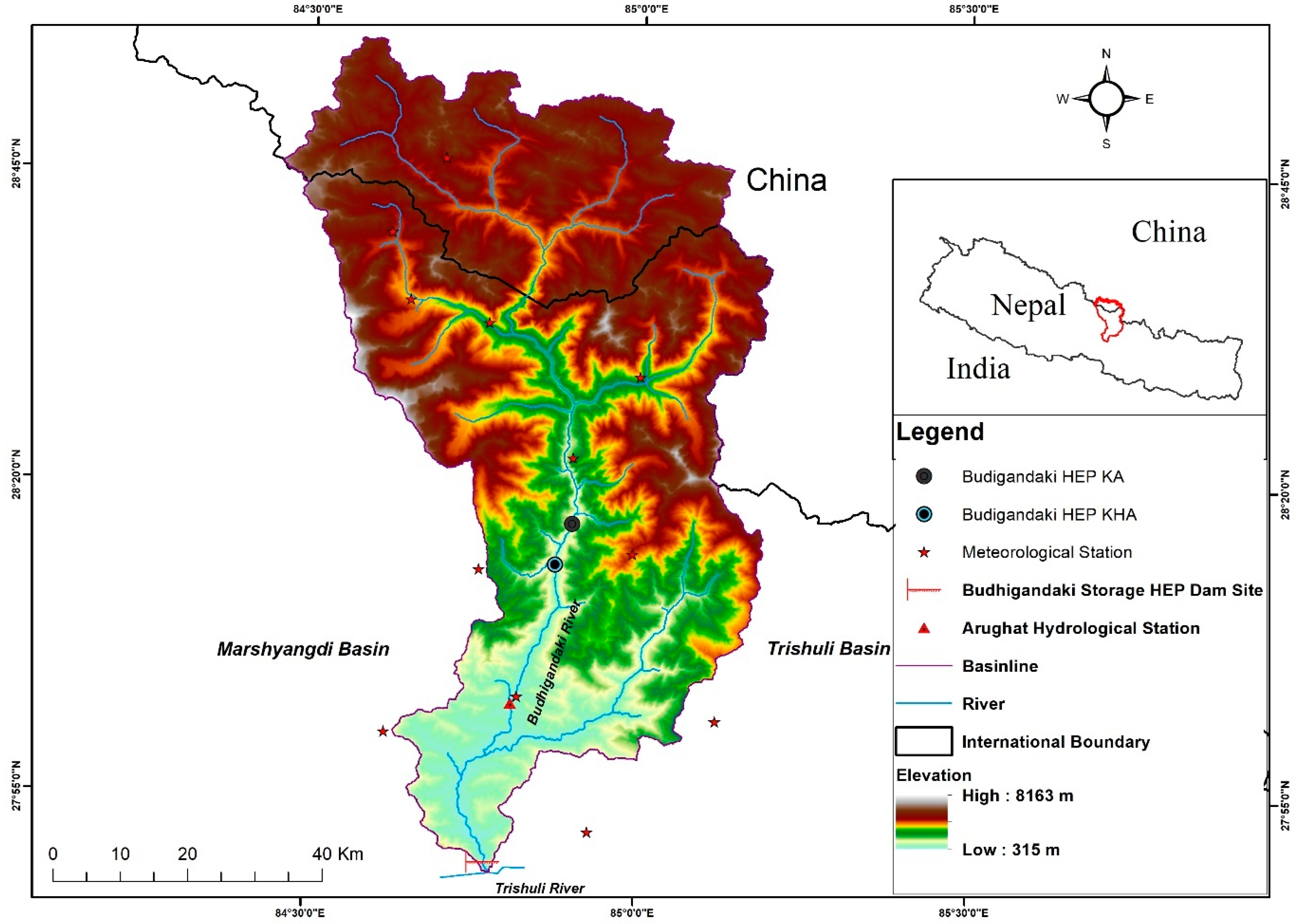
The BRB is a transboundary river basin of which about one-fourth of the basin area lies in Tibetan plateau of People’s Republic of China and the remaining part lies in Federal Democratic Republic of Nepal (Figure 1). The basin area at the confluence of Trishuli River is 4988 km2, with an average elevation of 3723 masl (range: 315 m–8163 m). Physiographically, the basin falls in the Middle Mountains and the Himalayas. It is noted here that Mount Manaslu, the eighth highest peak in the world, is situated in this basin [58]. Long-term annual rainfall of the BRB is 1495 mm with an extremely high spatial variability within the basin. Rainfall intensities vary throughout the basin with maximum intensity occurring on the south facing slopes of the mountains. The station Arughat receives an annual precipitation of greater than 2500 mm while the Tibetan part of the basin receives less than 700 mm [57,59]. The mean annual flow of the Budhigandaki river near the Budhigandaki Hydroelectric Project (BGHEP) dam site is estimated at 222 m3/s [53]. The temperature varies from −2.0 °C in winter to 33.0 °C in summer in the study basin [60].
2.2. Data Used
The hydro-meteorological data that has been used for the SWAT model in this study are precipitation, minimum and maximum air temperature. Besides, Digital Elevation Model (DEM), land use and soil map data are the spatial data required (Table 1).
2.2.1. Meteorological Data
Meteorological data from eight stations in and around the study basin (1981–2015) were used as input to the model (Figure 1). Two stations have both observed precipitation and temperature data while the remaining six stations have only precipitation data. Gridded data of precipitation and temperature for the Tibet part of the basin was also used in the study. Quality checking of the data was done through various methods: homogeneity test, outliers checking, inter parameter consistency checking, spatial checking and double mass curve analysis. The average areal precipitation over the catchment was calculated by the Thiessen polygon method [67] using geographic information system (GIS).
2.2.2. Flow Data
Long term daily flow data (1983–2012) of Budhigandaki river at Arughat gauging station has been used for calibration and validation of the model. Similarly, short term flow data available at the damsite of the proposed Budhigandaki Storage Hydropower Project (2013–2014) lying downstream of the Arughat station and headwork sites of two proposed run of the river hydropower projects, viz., Budhigandaki KA and KHA (2009) lying upstream of Arughat (Figure 1) were also used for additional validation of the model.
2.2.3. Spatial Data
Shuttle Radar Topography Mission (SRTM; 1 arc second horizontal resolution) DEM was used to delineate the river network and sub-basins. Landuse and land cover (LULC) data were obtained from [65]. Soil data of the Tibetan part of the basin was taken from Soil Terrain Database Programme (SOTER) which is at 1:1 million scale whereas soil data for Nepal was obtained from [65]. LULC and soil maps of the basin are shown in Figure 2a and b respectively. LULC data was categorized into nine classes while soil data was segregated into 17 classes. BRB is covered by snow and glaciers (SNGL-29%), followed by forest (FORS-23%), barren (BARN-21%), shrub and grassland (SHGR-18%) and agriculture (AGVT, AGST, AGLT-8%). River (RIVR) and residential built-up area (RESI) covers the least portion (~1%) of the total area. It can be seen from Figure 2b that hard rock mass in mountainous terrain (RockRock) covers a significant part (~33%) of the basin while inceptisols with loamy sand texture (IncSand) covers about 21% of the basin area. Gelic leptosols with rocky texture (LpiRock-13%) and gelic leptosols with loamy skeletal texture (LpiSkel-10%) are also found in different parts of BRB. Entisols with sandy texture (EntSand-7%), spodosols with sandy texture (SpoSand-5%), inceptisols with loamy texture (IncLoam-3%), alfisols with loamy texture (AlfLoam-3%) and eutric leptosols with rocky texture (LpeRock-3%) are also found in small patches. Inceptisols with loamy skeletal texture (IncSkel-1%), eutric leptosols with sandy texture (LpeSand-1%), entisols with loamy skeletal texture (EntSkel-0.5%), haplic luvisols with loamy texture (LvhLoam-0.4%), mollisols with sandy texture (MolSand-0.2%), leptosols with loamy texture (LpLoam < 0.1%), leptosols with loamy skeletal texture (LpmSkel < 0.1%) and entisols with loamy texture (Entloam < 0.1%) are found in traces.
2.3. SWAT Model
The Soil Water Assessment Tool (SWAT model) is a continuous-time, semi-distributed, process-based river basin simulation model operating on a daily or sub-daily time steps [68,69,70]. The basin is partitioned into a number of subbasins. Each sub-basin is further discretised into a number of hydrologic response units (HRUs), which are unique combinations of soil-landuse-slope exceeding a certain user defined threshold. Processes are simulated at HRU level and aggregated for each sub-basin, which are then routed through the river system using the variable storage or Muskingum method. SWAT facilitates an assortment of parameters defined at HRU, subbasin or basin level. The SWAT model simulates the various hydrological processes occurring in the river basin based on water balance within the basin as given by Equation (1).
where SWt is the final soil water content (mm), SW0 is the initial soil water content (mm), t is the time in days, Rday is the amount of precipitation on day i (mm), Qsurf is the amount of surface runoff on day i (mm), Ea is the amount of evapotranspiration on day i (mm), Wseep is the amount of water entering the vadose zone from soil profile on day i (mm), Qgw is the amount of return flow on day i (mm).
SWAT uses the climate data from the station nearest to the centroid of each sub-basin. A given precipitation is classified as solid (snow) and liquid (rainfall) based on a user-defined threshold value of mean air temperature. Snow melts when the maximum temperature on a given day exceeds the user defined threshold level. In snow covered areas, a fraction of the estimated daily potential evapotranspiration occurs by sublimation. Evaporation from soils and plants is computed separately by the model. Details of the SWAT model can be found in [30,70,71].
2.4. Model Setup and Simulation
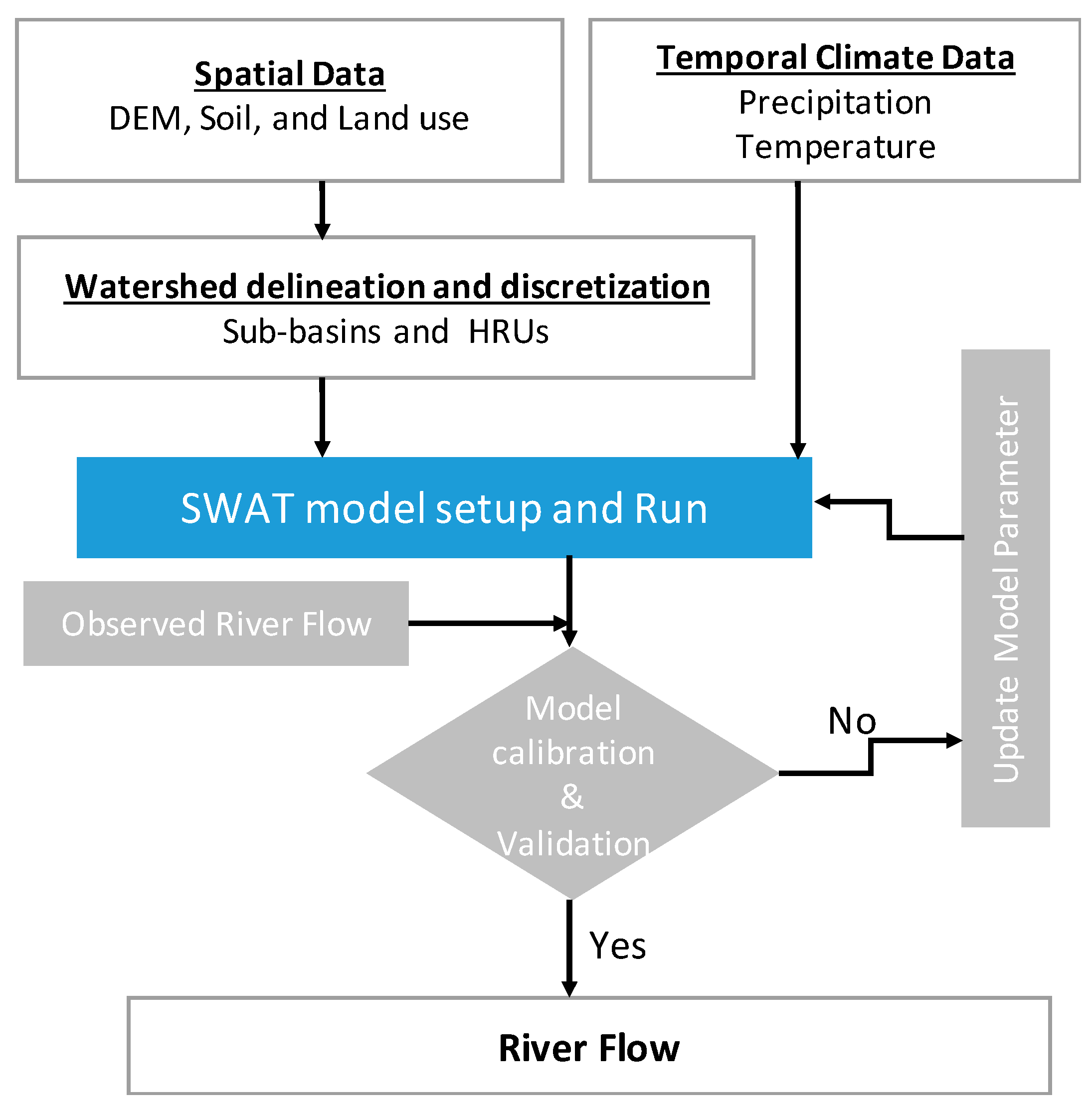
The BRB was divided into 16 sub-basins and five slope classes (0–30, 30–50, 50–70, 70–90 and >90 percent). A threshold value of 10% each for land use and land cover, soil (Figure 2) and slopes were used to divide the subbasin into unique 344 HRUs. Further, to account for orographic effects, we generated 500 m range elevation band in each sub basin. The methodological framework for model setup and simulation is given in Figure 3.
Precipitation and temperature data were fed into the model. Having a large number of missing flow data of years 2013 and 2014 at Arughat station and having 30 years [19,72,73,74] of relatively better data before 2013, observed flow data of Arughat station from 1981–2012 were used in the study. A warm up period (to stabilize the model initially) of 2 years (1981–1982) was excluded from the analysis. The model was calibrated using 20 years (two-thirds) of the study period (1983–2002) and validated using the remaining one-third i.e., 10 years (2003–2012). Based on the modeling experience in Nepalese basins and judgement of the study team, manual method was used for calibrating the model.
Surface runoff was estimated by the SCS curve number (SCS-CN) [75] method. The potential evapotranspiration was computed using Hargreaves method [76]. The computed runoff from each sub-basin was routed through the river network to the main basin outlet by using variable storage method.
Performance Evaluation Criteria
Moriasi et al. [77] has discussed various graphical and statistical model evaluation techniques. Among them, three well-established statistical indicators: Nash–Sutcliffe efficiency (NSE), percent bias (PBIAS), and ratio of the root mean square error to the standard deviation of measured data (RSR) were used in this study for model evaluation [69,77,78]. In addition to these three, Kling Gupta efficiency (KGE) prescribed by [79,80,81,82] has also been used for the purpose of evaluation.
Nash–Sutcliffe efficiency (NSE) is a normalized statistic that determines the relative magnitude of the residual variance (“noise”) compared to the measured data variance (“information”). NSE indicates how well the plot of observed versus simulated data fits the 1:1 line [83]. NSE is computed using Equation (2):
where, and are respectively observed and estimated discharge of day i, is the mean of the observed discharges. The optimum value is 1.0, with higher value indicating better model performance.
Percent bias (PBIAS) measures the average tendency of the simulated data to be larger or smaller than their observed counterparts. The optimal value of PBIAS is 0.0, with low-magnitude values indicating accurate model simulation. Positive values indicate model underestimation bias, and negative values indicate model overestimation bias [77]. PBIAS is, generally, expressed in percentage and is calculated using Equation (3).
where Vo and Ve are respectively the observed and simulated volumes of water for day i.
The root mean square error (RMSE) and the standard deviation of observed flow can be expressed as a ratio (RSR). It is commonly accepted that the lower the RMSE the better the model performance. RSR varies from the optimal value of 0, which indicates zero residual variation and therefore perfect model simulation, to a large positive value that indicates poorer model performance [77]. RSR is calculated using Equation (4).
The Kling–Gupta efficiency (KGE) that incorporates correlation, variability bias and mean bias [80] is increasingly used for model calibration and evaluation. It is expressed using Equation (5).
where, r is the correlation coefficient between the observed and simulated flows, and are standard deviations of observed and simulated flows respectively.
3. Results
3.1. Observed Rainfall-Runoff Characteristics
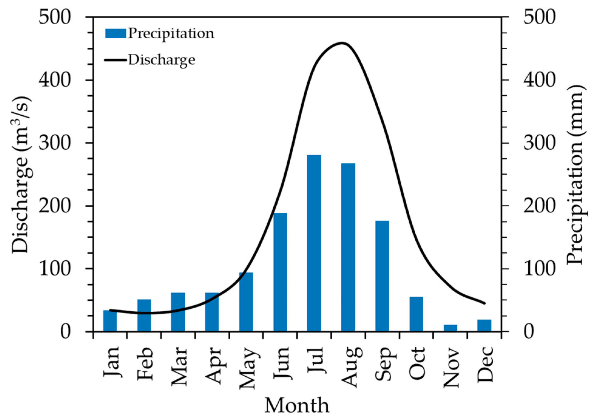
Long term monthly average precipitation and observed flow (1983–2012) based on Department of Hydrology and Meteorology (DHM) at Arughat gauging station is depicted in Figure 4. The figure shows that the flow closely follows the precipitation pattern of the basin. Long term annual basin precipitation has been calculated as 1301 mm (maximum 278 mm in July and minimum 11 mm in November). Similarly, the long-term average and standard deviation of the monthly flows are 163 m3/s and 156 m3/s, respectively.
3.2. SWAT Model Performance
The SWAT model was calibrated and validated manually for a simulation period of 30 years (1983–2012). The 15 most sensitive parameters were selected for calibration. The final adopted values of the parameters (in alphabetical order) are shown in Table 2. It can be seen that two different sets of parameters directly influence the surface runoff (CN2 and OV_N) and lateral flow (LAT_TIME and SURLAG) whereas five parameters (ALPHA_BF, GWDELAY, GWQMIN, SOL_AWC and SOL_Z) impact the baseflow from the basin. It is interesting to note that there are six snow related parameters (snowfall temperature (SFTMP), snowmelt temperature (SMTMP), snow cover (SNOCOVMX), degree-day factors (SMFMX, SMFMN) and temperature lapse rate (TLAPS)) which are used to calculate the snow component of the total flow. Thus, it is seen that the basin demonstrates a high degree of complexity among the different interacting components of the hydrological cycle.
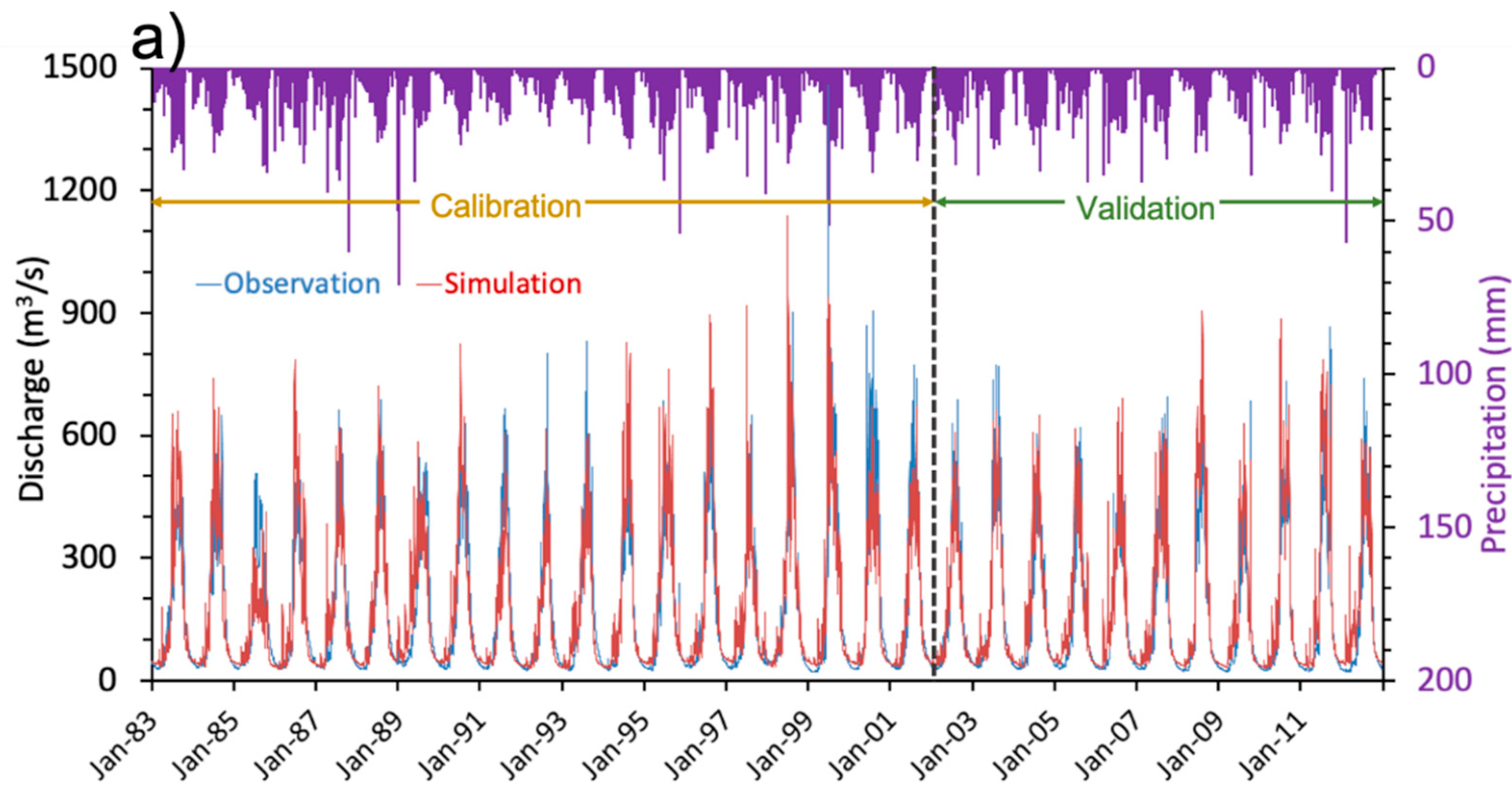
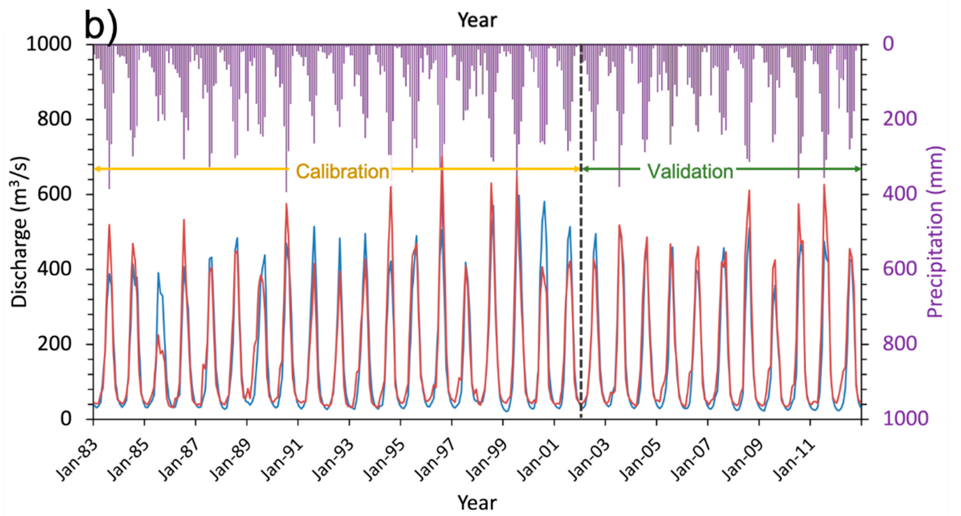
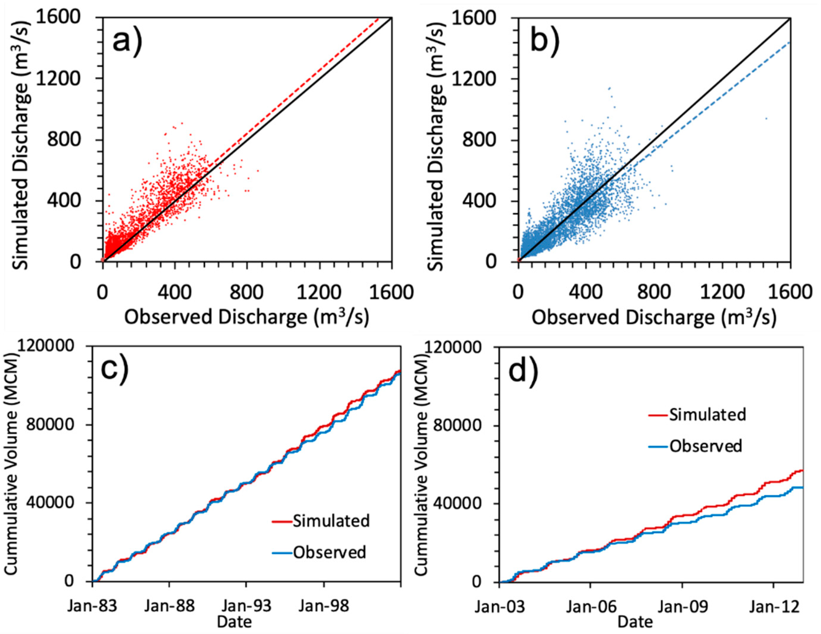
Simulated and observed hydrographs for the calibration and the validation periods at Arughat on daily and monthly time steps are shown in Figure 5. The mean and standard deviation of the observed (and simulated) flows are 168 (170) m3/s and 167 (168) m3/s, respectively for the calibration period and 154 (181) m3/s and 163 (180) m3/s, respectively for the validation period (Table 3). It can be seen from Figure 5 that the model simulates the flow pattern very well and the hydrographs are in good agreement with the rainfall pattern at daily and monthly timescales even for this length of time (20 years for calibration and 10 years for validation). It is also evident from the scatter plots of simulated vs. observed daily flows of these periods (Figure 6a,b). The difference in cumulative volume between the simulated and observed flow is very small for the calibration period (Figure 6c), however, the model has over-estimated the flow in the validation period (Figure 6d).
The NSE, PBIAS, RSR and KGE values for the calibration period are, respectively, 0.78, −1.46%, 0.47 and 0.89. Similarly, for the validation period, the values of NSE, PBIAS, RSR and KGE are 0.81, −17.1%, 0.44 and 0.79, respectively (Table 3). Based on the criteria prescribed by [77,80], all these indices fall in the ‘very good’ category except PBIAS in the validation period (‘satisfactory’ range). The graphical comparison (Figure 4, Figure 5 and Figure 6) and the performance rating (Table 3) show that the SWAT model is well calibrated and validated for the BRB at Arughat.
The monthly flows, both observed and simulated, for the period 1983–2012 are depicted in Figure 5b. The model performance parameters for monthly flows are 0.88 (NSE), −6.5% (PBIAS), 0.35 (RSR) and 0.91 (KGE). The graph and the performance statistics show that the calibrated SWAT model is capable of simulating the monthly flows well which is required for water availability studies in the BRB.
3.3. Additional Validation of SWAT at Supplementary Stations
Previous studies, e.g., [25,85] have used multi-site approach to calibrate the SWAT model. In the current study, the model is calibrated at a single point and validated at three supplementary points upstream and downstream of Arughat: (i) intake site of Budhigandaki KA (BG KA), (ii) intake site of Budhigandaki KHA (BG KHA) and (iii) 1200 MW Budhigandaki Hydroelectric Project (BGHEP) dam site (see Figure 1). It is to be noted that the study team carried out rigorous discharge measurements and prepared rating curves at these three locations during 2009–2010 (BG KA and BG KHA) and 2013–2014 (BGHEP damsite) which has been used for the additional validation. The results of the validation have been shown in Figure 7. The NSE, RSR, PBIAS and KGE values for BG KA are 0.66, 0.58, 21% and 0.59 and 0.58, 0.65, 13% and 0.54 for BG KHA, respectively. Similarly, their respective values for the BGHEP damsite are 0.91, 0.31, 7.88% and 0.81. As per the rating criteria by [77,80], the model performance is “very good” at the BGHEP dam site, “good” at BG KA and “satisfactory” at BG KHA. This independent validation at supplementary sites reveals that the calibrated model at Arughat can simulate the flow well for the Budhigandaki Basin up to the Trishuli confluence, although the performance is better in the downstream reach compared to the upstream reach.
3.4. Flow Duration Curve
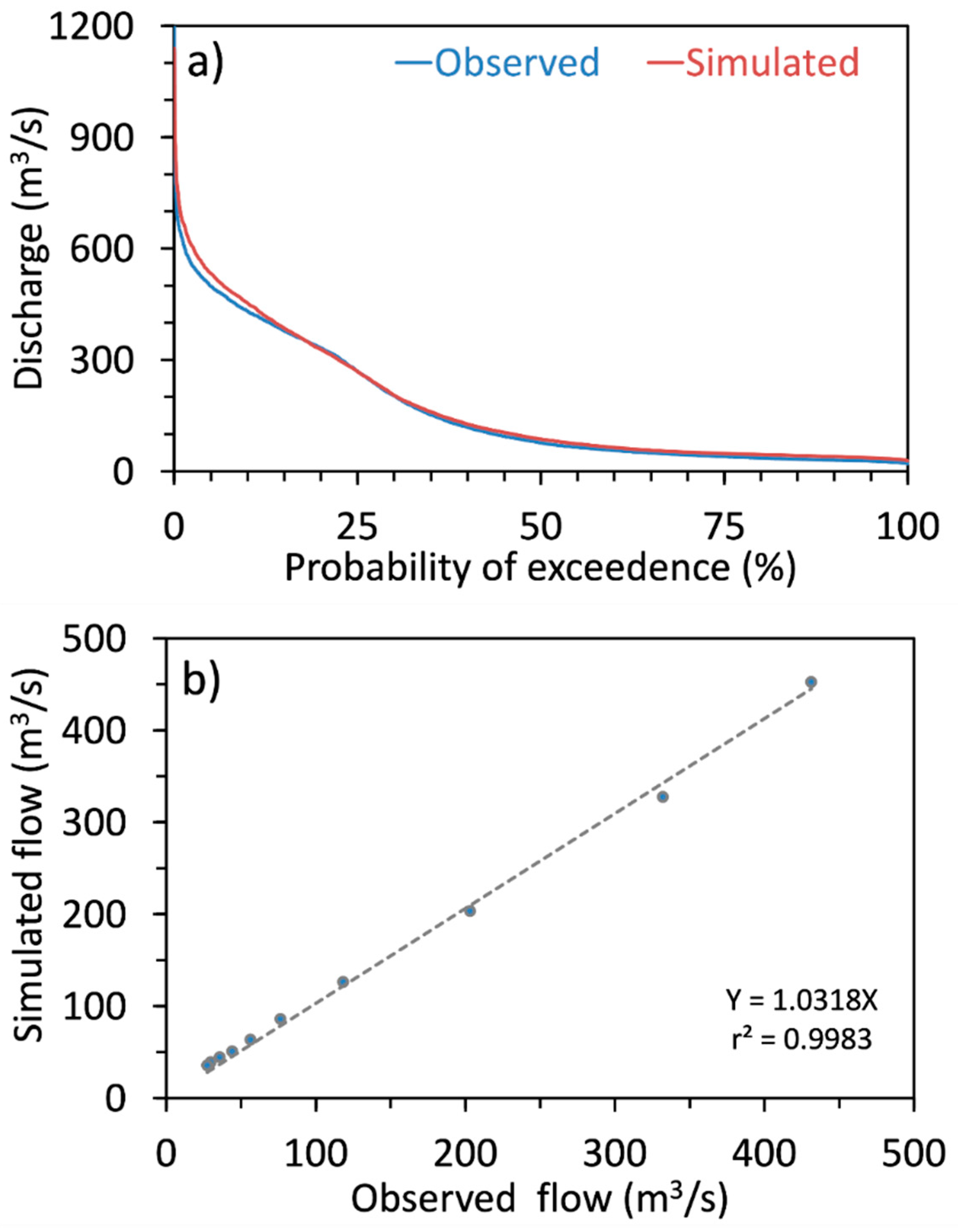
The flow-duration curve (FDC) is a probability discharge curve that shows the percentage of time in which a particular flow is equaled or exceeded [1]. FDC was prepared from the observed as well as simulated daily flow data at Arughat (Figure 8a). From the figure, it can be seen that the magnitude of the observed flows at 10%, 40% and 90% exceedance probabilities are 431, 118 and 29 m3/s respectively. Similarly, the exceedance probabilities are respectively 453, 126 and 39 m3/s for simulated flows. This indicates that the fractional difference between the corresponding values of the two flow-series are 5%, 7%, and 33%, respectively. The relationship between the simulated and observed values at 10 percentile exceedance intervals are plotted in Figure 8b. A very good linear correlation is found between these two series as indicated by the R2 value of 0.998.
3.5. Water Balance of the Budhigandaki Basin
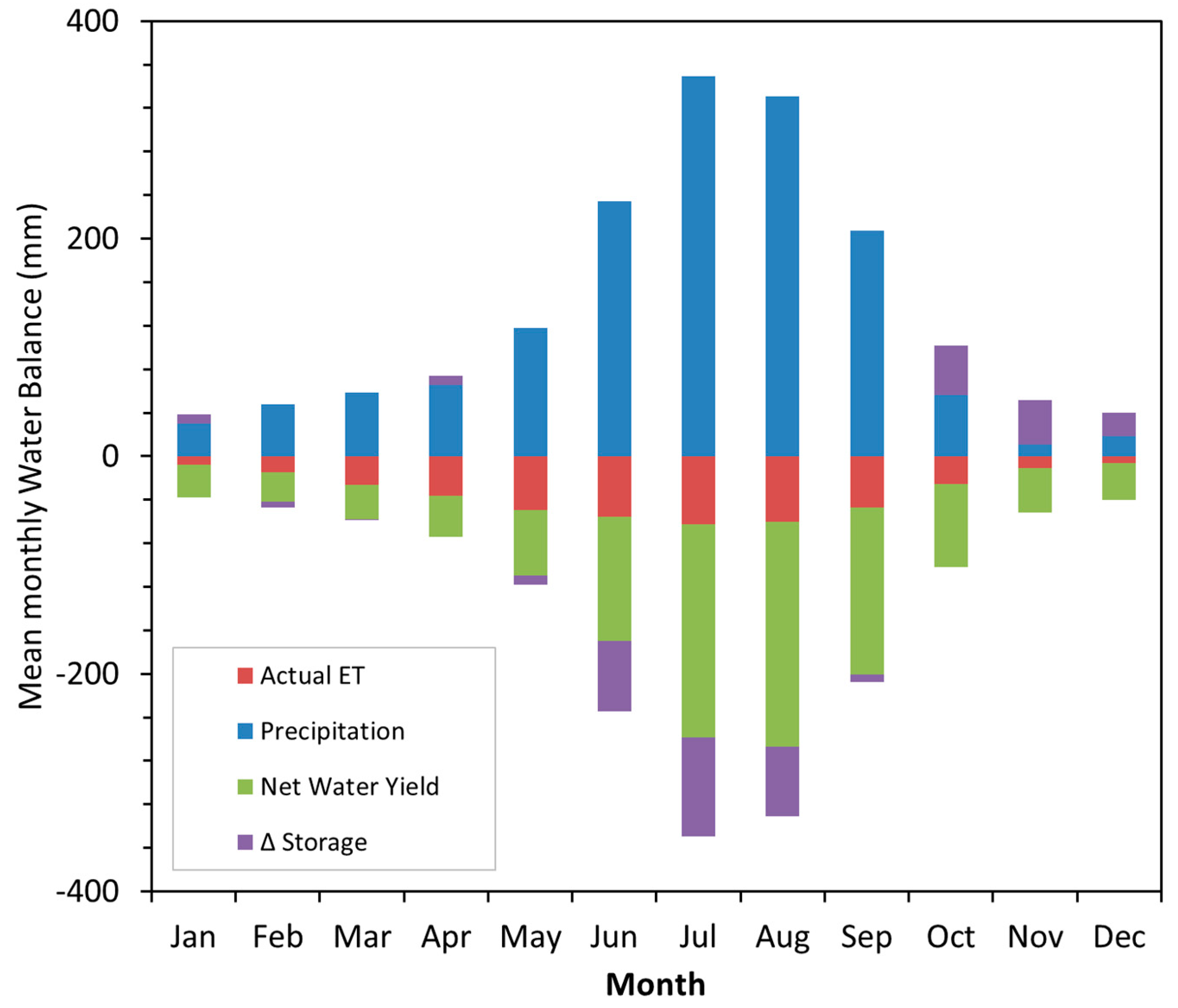
Monthly water balance of the BRB is shown in Figure 9. The figure depicts the distribution of water balance components, namely, precipitation (P), actual evapotranspiration (AET) and the net water yield (WY) of the study basin. The WY refers to the total flow coming as surface runoff, lateral flow, and groundwater flow minus transmission losses and pond abstractions [30]. Change in storage is defined as ∆Storage = −[(Precipitation (P) − Net Water Yield (WY) − Evapotranspiration (ET)]. It implies that if P > (WY + ET), the excess water infiltrates and is stored, as soil moisture and GW storages, of the basin. On the other hand, if (WY + ET) > P, the water deficit is met by soil and GW storages of the basin. For example, in January, some water is released from the basin to meet the WY and ET while it is stored in the soil and GW storage in July. It is noted here that ∆storage accounts for model errors too. It can be seen from the results that precipitation across the SWAT sub-basins varies from less than 700 mm (leeward side of northern Trans-Himalayan region) to above 2500 mm (foothills of the Himalayas). The average annual precipitation over the entire basin is 1528 mm. Here precipitation has been taken as the sum of annual rainfall and snowmelt (318 mm). The percentage of precipitation falling in pre-monsoon, monsoon, post monsoon and winter are respectively 16%, 74%, 4% and 6% of the total annual value. The average annual AET over the basin is 402 mm while WY is 1010 mm. The WY is about 56% during monsoon (June–September) while it is only 28% and 9% in pre-monsoon (March–May) and post-monsoon (October and November) seasons, respectively. It is only 7% of the total annual volume for the winter season (December–February). Delta storage for the entire simulation period has been calculated to be around 8%.
4. Discussion
In the BRB, the monsoon season (June–September) contributes approximately 74% of the total annual flow while the flow during the other eight months is only 26%. The highest flow occurs in August (23% of the total annual flow) while the lowest flow occurs in February (1.5%). The fractional difference between these two months was calculated to be more than 15, showing high runoff variability in the study basin. This value is comparable with other large and medium size basins of Nepal, for example, West Seti, Karnali, Trishuli, Narayani, Dudhkoshi and Sapta Koshi. The fractional differences of these basins range from 13 (West Seti at Gopighat and Sapta Koshi at Chatara) to 18 (Dudhkoshi at Rabuwa); flow contribution in monsoon season ranges from 72% to 77%, respectively. Furthermore, the low flow contribution is relatively higher in Karnali, West Seti and Saptakoshi (approximately 2%) while this is less than 1.5% in Dudhkoshi. It is interesting to note that low flow contribution is higher in the basins with a significant drainage area of Tibet and lying in the western part of Nepal.
The SWAT model was calibrated using 20 years (two-thirds) of the study period (1983–2002) and validated using the remaining one-third 10 years (2003–2012) which is comparable with the time period taken by [24]. The performance indices of this study are found better or comparable to similar studies carried out in other Nepalese basins. For example, for Chameliya, Karnali, Bheri, Kaligandaki, Indrawati, Tamakoshi, Arun and Tamor basins of Nepal, NSE (and PBIAS) values are respectively 0.75 (+5.1%), 0.84 (−14.2%), 0.70 (−4.4%), 0.78 (−4.0%), 0.72 (-), 0.76 (−1.7%), 0.81 (−6.8%) and 0.85 (+4.3%) for calibration period while these values are 0.65 (-9.3%), 0.84 (−15.4%), 0.71 (−8.9%), 0.8 (+9.6%), 0.87 (-), 0.84 (+5.2%), 0.58 (+24.6%) and 0.89 (+5.5%) respectively for validation period [25,40,45,47,51,85,86,87]. Similarly, NSE (and PBIAS) values of Gilgelabay basin of Ethiopia, Gurupura basin of India and Tizinafu basin of Western China were found to be respectively 0.69 (+4.8%), 0.83 (+17.5%) and 0.71 (+5.79%) for calibration period while these values for validation period were 0.68 (+4.9%), 0.85 (−3.9%) and 0.64 (−18.0%), respectively [88,89,90]. Moreover, [42] used SWAT model to simulate five glacierized mountain river basins of the world that includes the Narayani (Nepal), Vakhsh (Central Asia), Rhone (Switzerland), Mendoza (Central Andes, Argentina), and Chile (Central Dry Andes, Chile). The magnitudes of the statistical indicators of NSE, RSR and PBIAS of our study are comparable with this study.
Even though the model has simulated the flow very well in general, it has underestimated the high flow in some cases (e.g., 1992, 1993, 1999, 2000) while overestimated in some other cases (e.g., 1986, 2008) (Figure 5). The hydrographs in Figure 7a,b show the extended validation results which are based on the primary data collected at BG KA and BG KHA intake sites by the study team during 2009–2010. Figure 7c shows the simulated and observed hydrographs at BGHEP damsite for the year 2013–2014. The reference hydrological station (Arughat) is a few kilometers downstream and upstream from these points. It is to be noted here that the time of simulation for the Figure 7a–c are different. Data for the years 2013 and 2014 are not available at Arughat station for direct comparison. Nevertheless, it can be seen from Figure 5 that the flows for the years 2010, 2011 and 2012 are also overestimated by the model which is very much similar to the condition shown by Figure 7a,b. Further, the simulated flow data series in Figure 7c follows the precipitation pattern and as a result, the simulated hydrograph can be considered to be reasonable, although underestimated from the observed data. It is worth mentioning here that a longer simulation and observation period would add more confidence in the model performance at these locations. There are various factors that cause the difference in the observed and simulated flows that can be grouped into observation errors and model errors. Observation errors are attributed to (i) error in precipitation (human error while reading precipitation and instrumental error); (ii) inadequate rain-gauge stations to capture the spatial variation of precipitation including windward/leeward effect; (iii) error in water level reading; (iv) use of extrapolated stage-discharge relationship while calculating higher and lower flows; and (v) possible combinations of above [61,73,91,92,93,94]. In addition to observation errors discussed above, inherent limitations of SWAT flow calculation modules also affect simulated flows. Similarly, resolution of the DEM, land use and land cover, and soil types are only approximations of the real system. The differences between the observed and simulated flows at short timespans are found to be more compared to the long-term values. Despite these differences, the long-term values of the simulated and observed flows and their statistics are highly comparable.
In a water resources project, FDC is a useful tool to know the dependable flow while planning and designing engineering structures. For the BRB, the fractional difference between the simulated and observed low flows is seen to be high. However, the difference in the absolute values of the flows is considerably less compared to the high flows. Twenty-eight percent of the Budhigandaki River Basin is covered with snow and less than one percent (315 km2) is covered with glaciers. In the upper subbasins, the contribution of the glacier melt might affect the total runoff to some extent [95,96,97,98] whereas our area of interest lies in the lower part of BRB near Arughat (elevation 540 masl), where the contribution of glacier melt is insignificant in the total runoff. Past studies have modeled glacier melt in high altitude catchments above 3000 masl (for e.g., [95,97]) in which the calibration stations are also located in high elevations (Langtang at 3670 masl; catchment area 353 km2). Furthermore, from these studies it can be seen that the annual runoff quantified at the reference stations is around 9 m3/s while it is about 160 m3/s at Arughat. Thus, even a small contribution from glacier melt will have a huge impact on the high elevation stations while it will be less considerable at stations lying in lower elevations. There is some contribution of snowmelt flow during the pre-monsoon period whereas the base flow contribution is more in post monsoon period. It is to be noted that the precipitation contributes to net storage from May to September (wet period) and the storage depletes during most of the dry period from October to April. This causes the percentage of precipitation contribution to net water yield to be smaller during the monsoon period than the other three periods.
5. Conclusions
This study discretized the BRB into 16 sub-basins and 344 HRUs and developed a hydrological model in SWAT to characterize spatial and temporal distribution of water availability. Calibration and validation of the model was carried out at Arughat using daily flow data of 20 years and 10 years respectively. Even in such a long duration, the model performed well and was ranked “very good”. In addition to the conventional method of validation at the calibration station, this study further carried out validation at three supplementary points (two upstream and one downstream) at which the study team collected primary river flow data and prepared rating curves. Results of the supplementary validation further added confidence to the model performance.
This study estimated the mean annual flow at BRB outlet to be 240 m3/s with annual precipitation 1528 mm and AET approximately 26% of the precipitation. However, distinct seasonal variability is noted in the basin with precipitation varying from 67 mm (post-monsoon) to 1122 mm (monsoon), AET from 28 mm (winter) to 225 mm (monsoon), and WY from 92 mm (winter) to 670 mm (monsoon). The monsoon season contribution is 73%, 56%, and 66% in the average annual precipitation, AET, and WY, respectively in the BRB. Snowmelt contributes 20% of the total flow at the basin outlet during the pre-monsoon period and 8% in the post monsoon period. The magnitude of the simulated flows at 10%, 40% and 90% exceedance probabilities are 453, 126 and 39 m3/s respectively indicating high energy generation potential.
This study provides additional evidence to the SWAT diaspora of its applicability to simulate the rainfall-runoff characteristics of complex mountainous basin. Furthermore, the spatial and temporal variability in the available water of the BRB was estimated. The findings will be useful for hydrologists and planners in general to utilize the available water rationally in the times to come and particularly, to harness the hydroelectric potential of the basin.
Author Contributions
Conceptualization, S.M., D.A. and L.P.D.; methodology, S.M., D.A. and L.P.D.; software, validation, formal analysis, investigation, resources, data curation, writing—original draft preparation, S.M.; writing—review and editing, S.M., D.A. and L.P.D.; supervision, D.A. and L.P.D.; funding acquisition, D.A. All authors have read and agreed to the published version of the manuscript.
Funding
This research was funded by University Grants Commission (UGC), Nepal.
Institutional Review Board Statement
Not applicable.
Informed Consent Statement
Not applicable.
Data Availability Statement
The datasets used in this study can be accessed freely.
Acknowledgments
Authors would like to thank the Department of Hydrology and Meteorology, Government of Nepal for providing hydro-climatic data. The Budhigandaki Hydroelectric Project Development Committee is also acknowledged for providing hydrological data. The authors would like to thank three anonymous reviewers for constructive comments which helps to improve our manuscript substantially.
Conflicts of Interest
The authors declare no conflict of interest.
References
- Chow, V.T.; Maidment, D.R.; Mays, L.W. Applied Hydrology; TATA McGrawHill Inc.: New York, NY, USA, 1988. [Google Scholar]
- Zhang, Q.; Knowles, J.F.; Barnes, R.T.; Cowie, R.M.; Rock, N.; Williams, M.W. Surface and subsurface water contributions to streamflow from a mesoscale watershed in complex mountain terrain. Hydrol. Process. 2018, 32, 954–967. [Google Scholar] [CrossRef] [Green Version]
- Tallaksen, L.M. A review of baseflow recession analysis. J. Hydrol. 1995, 165, 349–370. [Google Scholar] [CrossRef]
- Dobriyal, P.; Badola, R.; Tuboi, C.; Hussain, S.A. A review of methods for monitoring streamflow for sustainable water resource management. Appl. Water Sci. 2017, 7, 2617–2628. [Google Scholar] [CrossRef] [Green Version]
- Loukas, A.; Vasiliades, L. Streamflow simulation methods for ungauged and poorly gauged watersheds. Nat. Hazards Earth Syst. Sci. 2014, 14, 1641–1661. [Google Scholar] [CrossRef] [Green Version]
- Shin, S.; Pokhrel, Y.; Talchabhadel, R.; Panthi, J. Spatio-temporal dynamics of hydrologic changes in the Himalayan river basins of Nepal using high-resolution hydrological-hydrodynamic modeling. J. Hydrol. 2021, 598, 126209. [Google Scholar] [CrossRef]
- Alford, D.; Armstrong, R.; Racoviteanu, A. Glacier Retreat in the Nepal Himalaya: The role of glaciers in stream flow from the Nepal Himalaya. World Bank Tech. Rep. Forthcom. 2011. [Google Scholar] [CrossRef]
- Hishinuma, S.; Takeuchi, K.; Magome, J. Challenges of hydrological analysis for water resource development in semi-arid mountainous regions: Case study in Iran. Hydrol. Sci. J. 2014, 59, 1718–1737. [Google Scholar] [CrossRef] [Green Version]
- Viviroli, D.; Dürr, H.H.; Messerli, B.; Meybeck, M.; Weingartner, R. Mountains of the world, water towers for humanity: Typology, mapping, and global significance. Water Resour. Res. 2007, 43. [Google Scholar] [CrossRef] [Green Version]
- Horton, R.E. Drainage-basin characteristics. EOS Trans. Am. Geophys. Union 1932, 13, 350–361. [Google Scholar] [CrossRef]
- Kale, V.S. Fluvial geomorphology of Indian rivers: An overview. Prog. Phys. Geogr. 2002, 26, 400–433. [Google Scholar] [CrossRef]
- Higuchi, K.; Ageta, Y.; Yasunari, T.; Inoue, J. Characteristics of precipitation during the monsoon season in high-mountain areas of the Nepal Himalaya. IAHS Publ. 1982, 138, 21–30. [Google Scholar]
- Shrestha, A.B.; Wake, C.P.; Dibb, J.E.; Mayewski, P.A. Precipitation fluctuations in the Nepal Himalaya and its vicinity and relationship with some large scale climatological parameters. Int. J. Climatol. J. R. Meteorol. Soc. 2000, 20, 317–327. [Google Scholar] [CrossRef]
- Kansakar, S.R.; Hannah, D.M.; Gerrard, J.; Rees, G. Spatial pattern in the precipitation regime of Nepal. Int. J. Climatol. J. R. Meteorol. Soc. 2004, 24, 1645–1659. [Google Scholar] [CrossRef]
- Putkonen, J.K. Continuous Snow and Rain Data at 500 to 4400 m Altitude near Annapurna, Nepal, 1999–2001. Arct. Antarct. Alp. Res. 2004, 36, 244–248. [Google Scholar] [CrossRef]
- Ichiyanagi, K.; Yamanaka, M.D.; Muraji, Y.; Vaidya, B.K. Precipitation in Nepal between 1987 and 1996. Int. J. Climatol. J. R. Meteorol. Soc. 2007, 27, 1753–1762. [Google Scholar] [CrossRef]
- Devkota, R.P.; Pandey, V.P.; Bhattarai, U.; Shrestha, H.; Adhikari, S.; Dulal, K.N. Climate change and adaptation strategies in Budhi Gandaki River Basin, Nepal: A perception-based analysis. Clim. Chang. 2017, 140, 195–208. [Google Scholar] [CrossRef]
- Pokharel, B.; Wang, S.S.; Meyer, J.; Marahatta, S.; Nepal, B.; Chikamoto, Y.; Gillies, R. The east–west division of changing precipitation in Nepal. Int. J. Climatol. 2020, 40, 3348–3359. [Google Scholar] [CrossRef]
- WMO. Calculation of Monthly and Annual 30-Year Standard Normals, Prepared by a Meeting of Experts, Washington, DC, USA, March 1989; WCDP-No. 10, WMO-TD/No. 341; World Meteorological Organization: Geneva, Switzerland, 1989. [Google Scholar]
- Jain, S.K.; Jain, S.K.; Jain, N.; Xu, C.-Y. Hydrologic modeling of a Himalayan mountain basin by using the SWAT mode. Hydrol. Earth Syst. Sci. Discuss. 2017, 1–26. [Google Scholar] [CrossRef] [Green Version]
- Woolridge, D.D.; Niemann, J.D. Mountain Basin Hydrologic Study. 2018. Available online: https://dnrweblink.state.co.us/dwr/0/edoc/3377613/DWR_3377613.pdf?searchid=10250736-fd55-4a8f-a43f-b9270fad6e92 (accessed on 22 December 2020).
- Meng, F.; Sa, C.; Liu, T.; Luo, M.; Liu, J.; Tian, L. Improved Model Parameter Transferability Method for Hydrological Simulation with SWAT in Ungauged Mountainous Catchments. Sustainability 2020, 12, 3551. [Google Scholar] [CrossRef]
- Marahatta, S.; Devkota, L.; Aryal, D. Hydrological Modeling: A Better Alternative to Empirical Methods for Monthly Flow Estimation in Ungauged Basins. J. Water Resour. Prot. 2021, 254–270. [Google Scholar] [CrossRef]
- Abbaspour, K.C.; Rouholahnejad, E.; Vaghefi, S.; Srinivasan, R.; Yang, H.; Kløve, B. A continental-scale hydrology and water quality model for Europe: Calibration and uncertainty of a high-resolution large-scale SWAT model. J. Hydrol. 2015, 524, 733–752. [Google Scholar] [CrossRef] [Green Version]
- Pandey, V.P.; Dhaubanjar, S.; Bharati, L.; Thapa, B.R. Spatio-temporal distribution of water availability in Karnali-Mohana Basin, Western Nepal: Hydrological model development using multi-site calibration approach (Part-A). J. Hydrol. Reg. Stud. 2020, 29, 100690. [Google Scholar] [CrossRef]
- Zhou, X.; Helmers, M.; Qi, Z. Modeling of subsurface tile drainage using MIKE SHE. Appl. Eng. Agric. 2013, 29, 865–873. [Google Scholar]
- Devkota, L.P.; Gyawali, D.R. Impacts of climate change on hydrological regime and water resources management of the Koshi River Basin, Nepal. J. Hydrol. Reg. Stud. 2015, 4, 502–515. [Google Scholar] [CrossRef] [Green Version]
- Sitterson, J.; Knightes, C.; Parmar, R.; Wolfe, K.; Avant, B.; Muche, M. An Overview of Rainfall-Runoff Model Types. 2018. Available online: https://cfpub.epa.gov/si/si_public_record_report.cfm?dirEntryId=339328&Lab=NERL (accessed on 12 January 2021).
- Hossain, S.; Hewa, G.A.; Wella-Hewage, S. A Comparison of continuous and event-based rainfall–runoff (RR) modelling using EPA-SWMM. Water 2019, 11, 611. [Google Scholar] [CrossRef] [Green Version]
- Arnold, J.G.; Srinivasan, R.; Muttiah, R.S.; Williams, J.R.; Ramanarayanan, T.S.; Arnold, J.G.; Bednarz, S.T.; Srinivasan, R.; Muttiah, R.S.; Williams, J.R. Large area hydrologic modeling and assessment part I: Model development 1. JAWRA J. Am. Water Resour. Assoc. 1998, 34, 73–89. [Google Scholar] [CrossRef]
- Williams, J.R.; Arnold, J.G.; Kiniry, J.R.; Gassman, P.W.; Green, C.H. History of model development at Temple, Texas. Hydrol. Sci. J. 2008, 53, 948–960. [Google Scholar] [CrossRef] [Green Version]
- Douglas-Mankin, K.R.; Srinivasan, R.; Arnold, J.G. Soil and Water Assessment Tool (SWAT) model: Current developments and applications. Trans. ASABE 2010, 53, 1423–1431. [Google Scholar] [CrossRef]
- Tan, M.L.; Gassman, P.W.; Srinivasan, R.; Arnold, J.G.; Yang, X. A review of SWAT studies in Southeast Asia: Applications, challenges and future directions. Water 2019, 11, 914. [Google Scholar] [CrossRef] [Green Version]
- Das, B.; Jain, S.; Singh, S.; Thakur, P. Evaluation of multisite performance of SWAT model in the Gomti River Basin, India. Appl. Water Sci. 2019, 9, 1–10. [Google Scholar] [CrossRef] [Green Version]
- Van Griensven, A.; Ndomba, P.; Yalew, S.; Kilonzo, F. Critical review of SWAT applications in the upper Nile basin countries. Hydrol. Earth Syst. Sci. 2012, 16, 3371–3381. [Google Scholar] [CrossRef] [Green Version]
- Fukunaga, D.C.; Cecílio, R.A.; Zanetti, S.S.; Oliveira, L.T.; Caiado, M.A.C. Application of the SWAT hydrologic model to a tropical watershed at Brazil. Catena 2015, 125, 206–213. [Google Scholar] [CrossRef]
- Anand, J.; Gosain, A.K.; Khosa, R.; Srinivasan, R. Regional scale hydrologic modeling for prediction of water balance, analysis of trends in streamflow and variations in streamflow: The case study of the Ganga River basin. J. Hydrol. Reg. Stud. 2018, 16, 32–53. [Google Scholar] [CrossRef]
- Tang, X.; Zhang, J.; Gao, C.; Ruben, G.B.; Wang, G. Assessing the uncertainties of four precipitation products for swat modeling in Mekong River basin. Remote Sens. 2019, 11, 304. [Google Scholar] [CrossRef] [Green Version]
- CARD (Center for Agricultural and Rural Development). Swat Lit. Database Peer-Reviewed J. Artic; Center for Agricultural and Rural Development—Iowa State University: Ames, IA, USA, 2020; Available online: https://www.card.iastate.edu/swatarticles (accessed on 13 January 2021).
- Shrestha, S.; Shrestha, M.; Shrestha, P.K. Evaluation of the SWAT model performance for simulating river discharge in the Himalayan and tropical basins of Asia. Hydrol. Res. 2018, 49, 846–860. [Google Scholar] [CrossRef] [Green Version]
- Bharati, L.; Gurung, P.; Jayakody, P.; Smakhtin, V.; Bhattarai, U. The projected impact of climate change on water availability and development in the Koshi Basin, Nepal. Mt. Res. Dev. 2014, 34, 118–130. [Google Scholar] [CrossRef]
- Omani, N.; Srinivasan, R.; Karthikeyan, R.; Smith, P.K. Hydrological modeling of highly glacierized basins (Andes, Alps, and Central Asia). Water 2017, 9, 111. [Google Scholar] [CrossRef] [Green Version]
- Talchabhadel, R.; Nakagawa, H.; Kawaike, K.; Yamanoi, K.; Aryal, A.; Bhatta, B.; Karki, S. SWAT modeling for assessing future scenarios of soil erosion in West Rapti River Basin of Nepal. In Proceedings of the EGU General Assembly Conference Abstracts, Online, 4–8 May 2020; p. 1853. [Google Scholar]
- Dhami, B.; Himanshu, S.K.; Pandey, A.; Gautam, A.K. Evaluation of the SWAT model for water balance study of a mountainous snowfed river basin of Nepal. Environ. Earth Sci. 2018, 77. [Google Scholar] [CrossRef]
- Mishra, Y.; Nakamura, T.; Babel, M.S.; Ninsawat, S.; Ochi, S. Impact of climate change on water resources of the Bheri River Basin, Nepal. Water 2018, 10, 220. [Google Scholar] [CrossRef] [Green Version]
- Dahal, P.; Shrestha, M.L.; Panthi, J.; Pradhananga, D. Modeling the future impacts of climate change on water availability in the Karnali River Basin of Nepal Himalaya. Environ. Res. 2020, 185, 109430. [Google Scholar] [CrossRef]
- Bajracharya, A.R.; Bajracharya, S.R.; Shrestha, A.B.; Maharjan, S.B. Climate change impact assessment on the hydrological regime of the Kaligandaki Basin, Nepal. Sci. Total Environ. 2018, 625, 837–848. [Google Scholar] [CrossRef]
- Lamichhane, S.; Shakya, N.M. Integrated assessment of climate change and land use change impacts on hydrology in the Kathmandu Valley watershed, Central Nepal. Water 2019, 11, 2059. [Google Scholar] [CrossRef] [Green Version]
- Dahal, V.; Shakya, N.M.; Bhattarai, R. Estimating the impact of climate change on water availability in Bagmati Basin, Nepal. Environ. Process. 2016, 3, 1–17. [Google Scholar] [CrossRef]
- Pandey, V.P.; Dhaubanjar, S.; Bharati, L.; Thapa, B.R. Spatio-temporal distribution of water availability in Karnali-Mohana Basin, Western Nepal: Climate change impact assessment (Part-B). J. Hydrol. Reg. Stud. 2020, 29, 100691. [Google Scholar] [CrossRef]
- Bhatta, B.; Shrestha, S.; Shrestha, P.K.; Talchabhadel, R. Evaluation and application of a SWAT model to assess the climate change impact on the hydrology of the Himalayan River Basin. Catena 2019, 181, 104082. [Google Scholar] [CrossRef]
- Bharati, L.; Gurung, P.; Maharjan, L.; Bhattarai, U. Past and future variability in the hydrological regime of the Koshi Basin, Nepal. Hydrol. Sci. J. 2016, 61, 79–93. [Google Scholar] [CrossRef] [Green Version]
- BGHEP. Feasibility Study and Detailed Design of Budhigandaki Hydropower Project Part 1; Budhigandaki Hydroelectric Project Development Committee, Government of Nepal: Kathmandu, Nepal, 2015.
- Khatri, H.B.; Jain, M.K.; Jain, S.K. Modelling of streamflow in snow dominated Budhigandaki catchment in Nepal. J. Earth Syst. Sci. 2018, 127, 1–14. [Google Scholar] [CrossRef] [Green Version]
- Pangali Sharma, T.P.; Zhang, J.; Khanal, N.R.; Prodhan, F.A.; Paudel, B.; Shi, L.; Nepal, N. Assimilation of snowmelt runoff model (SRM) using satellite remote sensing data in Budhi Gandaki River Basin, Nepal. Remote Sens. 2020, 12, 1951. [Google Scholar] [CrossRef]
- Shrestha, M.L. Interannual variation of summer monsoon rainfall over Nepal and its relation to Southern Oscillation Index. Meteorol. Atmos. Phys. 2000, 75, 21–28. [Google Scholar] [CrossRef]
- Marahatta, S.; Dangol, B.S.; Gurung, G.B. Temporal and Spatial Variability of Climate Change over Nepal, 1976–2005; Practical Action Nepal Office: Kathmandu, Nepal, 2009; ISBN 9937813522. [Google Scholar]
- MoCTCA. Mountaineering in Nepal Facts and Figures; Ministry of Culture, Tourism and Civil Aviation (MoCTCA), Government of Nepal: Kathmandu, Nepal, 2014.
- DHM. Study of Climate and Climatic Variation over Nepal; Technical Report; Department of Hydrology and Meteorology, Government of Nepal: Kathmandu, Nepal, 2015.
- DHM. Institutional Development of Department of Hydrology and Meteorology; Technical Report No.7 (Basin Study); DHM: Kathmandu, Nepal, 2002. [Google Scholar]
- DHM. Streamflow Summary (1962–2015); Department of Hydrology and Meteorology, Government of Nepal: Kathmandu, Nepal, 2018.
- NNH. Hydrology, Hydraulics and Sediment Studies of Budhigandaki KA HEP; Naulo Nepal Hydro-electric (P) Ltd.: Kaski District, Nepal, 2010. [Google Scholar]
- NNH. Hydrology, Hydraulics and Sediment Studies of Budhigandaki KHA HEP; Naulo Nepal Hydro-electric (P) Ltd.: Kaski District, Nepal, 2010. [Google Scholar]
- Yang, K.; He, J. China Meteorological Forcing Dataset (1979−2018). National Tibetan Plateau Data Center, 2019. Available online: https://doi:10.11888/AtmosphericPhysics.tpe.249369.file (accessed on 29 May 2021).
- DoWRI Irrigation Master Plan Preparation through Integrated River Basin Planning (Dataset), Water Resources Project Preparatory Facility; Department of Water Resources and Irrigation, Ministry of Energy, Water Resources and Irrigation (MoEWRI): Kathmandu, Nepal, 2019.
- ICIMOD. Land Cover of Nepal 2010 [Dataset]; International Center for Integrated Mountain Development (ICIMOD): Kathmandu, Nepal, 2010; Available online: http://rds.icimod.org/Home/DataDetail (accessed on 3 December 2020).
- Thiessen, A.H. Precipitation averages for large areas. Mon. Weather Rev. 1911, 39, 1082–1089. [Google Scholar] [CrossRef]
- Srinivasan, R.; Ramanarayanan, T.S.; Arnold, J.G.; Bednarz, S.T. Large area hydrologic modeling and assessment part II: Model application 1. J. Am. Water Resour. Assoc. 1998, 34, 91–101. [Google Scholar] [CrossRef]
- Moriasi, D.N.; Wilson, B.N.; Douglas-Mankin, K.R.; Arnold, J.G.; Gowda, P.H. Hydrologic and water quality models: Use, calibration, and validation. Trans. ASABE 2012, 55, 1241–1247. [Google Scholar] [CrossRef]
- Van Liew, M.W.; Arnold, J.G.; Bosch, D.D. Problems and potential of autocalibrating a hydrologic model. Trans. ASAE 2005, 48, 1025–1040. [Google Scholar] [CrossRef] [Green Version]
- Neitsch, S.L.; Arnold, J.G.; Kiniry, J.R.; Williams, J.R. Soil and Water Assessment Tool Theoretical Documentation Version 2009; Texas Water Resources Institute: College Station, TX, USA, 2011. [Google Scholar]
- WMO. The Role of Climatological Normals in a Changing Climate; WCDMP-No. 61, WMO-TD No. 1377; World Meteorological Organization: Geneva, Switzerland, 2007. [Google Scholar]
- WMO. Guide to Climatological Practices; 2011 Edition, WMO Number 100; World Meteorological Organization: Geneva, Switzerland, 2011. [Google Scholar]
- WMO. Guidelines on the Calculation of Climate Normals; 2017 Edition WMO-No. 1203; World Meteorological Organization: Geneva, Switzerland, 2017. [Google Scholar]
- Mockus, V. National Engineering Handbook; Soil Conservation Service: Washington, DC, USA, 1964; Volume 4. [Google Scholar]
- Hargreaves, G.H.; Samani, Z.A. Estimating potential evapotranspiration. J. Irrig. Drain. Div. 1982, 108, 225–230. [Google Scholar] [CrossRef]
- Moriasi, D.N.; Arnold, J.G.; Van Liew, M.W.; Bingner, R.L.; Harmel, R.D.; Veith, T.L. Model evaluation guidelines for systematic quantification of accuracy in watershed simulations. Trans. ASABE 2007, 50, 885–900. [Google Scholar] [CrossRef]
- Moriasi, D.N.; Gitau, M.W.; Pai, N.; Daggupati, P. Hydrologic and water quality models: Performance measures and evaluation criteria. Trans. ASABE 2015, 58, 1763–1785. [Google Scholar]
- Schaefli, B.; Gupta, H.V. Do Nash values have value? Hydrol. Process. An Int. J. 2007, 21, 2075–2080. [Google Scholar] [CrossRef] [Green Version]
- Gupta, H.V.; Kling, H.; Yilmaz, K.K.; Martinez, G.F. Decomposition of the mean squared error and NSE performance criteria: Implications for improving hydrological modelling. J. Hydrol. 2009, 377, 80–91. [Google Scholar] [CrossRef] [Green Version]
- Knoben, W.J.M.; Freer, J.E.; Woods, R.A. Inherent benchmark or not? Comparing Nash–Sutcliffe and Kling–Gupta efficiency scores. Hydrol. Earth Syst. Sci. 2019, 23, 4323–4331. [Google Scholar] [CrossRef] [Green Version]
- Pool, S.; Vis, M.; Seibert, J. Evaluating model performance: Towards a non-parametric variant of the Kling-Gupta efficiency. Hydrol. Sci. J. 2018, 63, 1941–1953. [Google Scholar] [CrossRef]
- Nash, J.E.; Sutcliffe, J.V. River flow forecasting through conceptual models part I—A discussion of principles. J. Hydrol. 1970, 10, 282–290. [Google Scholar] [CrossRef]
- Arnold, J.G.; Kiniry, J.R.; Srinivasan, R.; Williams, J.R.; Haney, E.B.; Neitsch, S.L. Soil & Water Assessment Tool: Input/Output Documentation; Version 2012; TR-439; Texas Water Resources Institute: Forney, TX, USA, 2013; p. 650. [Google Scholar]
- Bharati, L.; Bhattarai, U.; Khadka, A.; Gurung, P.; Neumann, L.E.; Penton, D.J.; Dhaubanjar, S.; Nepal, S. From the Mountains to the Plains: Impact of Climate Change on Water Resources in the Koshi River Basin; International Water Management Institute (IWMI): Colombo, Sri Lanka, 2019; Volume 187, ISBN 9290908858. [Google Scholar]
- Pandey, V.P.; Dhaubanjar, S.; Bharati, L.; Thapa, B.R. Hydrological response of Chamelia watershed in Mahakali Basin to climate change. Sci. Total Environ. 2019, 650, 365–383. [Google Scholar] [CrossRef]
- Palazzoli, I.; Maskey, S.; Uhlenbrook, S.; Nana, E.; Bocchiola, D. Impact of prospective climate change on water resources and crop yields in the Indrawati basin, Nepal. Agric. Syst. 2015, 133, 143–157. [Google Scholar] [CrossRef]
- Tegegne, G.; Park, D.K.; Kim, Y.-O. Comparison of hydrological models for the assessment of water resources in a data-scarce region, the Upper Blue Nile River Basin. J. Hydrol. Reg. Stud. 2017, 14, 49–66. [Google Scholar] [CrossRef]
- Sharannya, T.M.; Mudbhatkal, A.; Mahesha, A. Assessing climate change impacts on river hydrology–A case study in the Western Ghats of India. J. Earth Syst. Sci. 2018, 127, 1–11. [Google Scholar] [CrossRef] [Green Version]
- Duan, Y.; Liu, T.; Meng, F.; Luo, M.; Frankl, A.; De Maeyer, P.; Bao, A.; Kurban, A.; Feng, X. Inclusion of modified snow melting and flood processes in the swat model. Water 2018, 10, 1715. [Google Scholar] [CrossRef] [Green Version]
- Le Coz, J. A Literature Review of Methods for Estimating the Uncertainty Associated with Stage-Discharge Relations. WMO Rep. PO6a 2012, 21. Available online: https://www.semanticscholar.org/paper/A-literature-review-of-methods-for-estimating-the-Coz-Cemagref/b685243d91acd17a64c3e31ecff08ea39d5b279d (accessed on 14 January 2021).
- Subramanayam, K. Engineering Hydrology; TATA McGraw Hills Publications Ltd.: New Delhi, India, 1994; ISBN 0-07-462449-8. [Google Scholar]
- Domeneghetti, A.; Castellarin, A.; Brath, A. Assessing rating-curve uncertainty and its effects on hydraulic model calibration. Hydrol. Earth Syst. Sci. 2012, 16, 1191–1202. [Google Scholar] [CrossRef] [Green Version]
- Manfreda, S.; Pizarro, A.; Moramarco, T.; Cimorelli, L.; Pianese, D.; Barbetta, S. Potential advantages of flow-area rating curves compared to classic stage-discharge-relations. J. Hydrol. 2020, 585, 124752. [Google Scholar] [CrossRef]
- Kayastha, R.B.; Steiner, N.; Kayastha, R.; Mishra, S.K.; Forster, R.R. Comparative Study of Hydrology and Icemelt in Three Nepal River Basins Using the Glacio-Hydrological Degree-Day Model (GDM) and Observations from the Advanced Scatterometer (ASCAT). Front. Earth Sci. 2020, 7, 354. [Google Scholar] [CrossRef] [Green Version]
- Mishra, S.K.; Hayse, J.; Veselka, T.; Yan, E.; Kayastha, R.B.; LaGory, K.; McDonald, K.; Steiner, N. An integrated assessment approach for estimating the economic impacts of climate change on River systems: An application to hydropower and fisheries in a Himalayan River, Trishuli. Environ. Sci. Policy 2018, 87, 102–111. [Google Scholar] [CrossRef]
- Pradhananga, N.S.; Kayastha, R.B.; Bhattarai, B.C.; Adhikari, T.R.; Pradhan, S.C.; Devkota, L.P.; Shrestha, A.B.; Mool, P.K. Estimation of discharge from Langtang River basin, Rasuwa, Nepal, using a glacio-hydrological model. Ann. Glaciol. 2014, 55, 223–230. [Google Scholar] [CrossRef] [Green Version]
- Khadka, M.; Kayastha, R.B.; Kayastha, R. Future projection of cryospheric and hydrologic regimes in Koshi River basin, Central Himalaya, using coupled glacier dynamics and glacio-hydrological models. J. Glaciol. 2020. [Google Scholar] [CrossRef]
Figure 1.
Location map of the Budhigandki River Basin.

Figure 2.
(a) Landuse and Land Cover, (b) Soil Map.

Figure 3.
Methodological framework for application of SWAT hydrological model.

Figure 4.
Long term rainfall-runoff pattern of the Budhigandaki River Basin at Arughat.

Figure 5.
Simulated (red line) and observed (blue line) hydrograph for calibration (1983–2002) and validation period (2003–2012) at Arughat Station. Upper panel (a) shows the daily and lower panel; (b) shows the monthly simulation results. Precipitation data are shown in the inverted secondary y-axis as purple bars.


Figure 6.
Scattered plots for daily flow in (a) calibration and; (b) validation; cumulative volume balance in the (c) calibration period; and the (d) validation period.
Figure 6.
Scattered plots for daily flow in (a) calibration and; (b) validation; cumulative volume balance in the (c) calibration period; and the (d) validation period.

Figure 7.
Additional validation of flows at supplementary stations in daily time step: (a) Budhigandaki KA, (b) Budhigandaki KHA and (c) BGHEP dam site. Precipitation data are shown in the inverted secondary y-axis as purple bars.
Figure 7.
Additional validation of flows at supplementary stations in daily time step: (a) Budhigandaki KA, (b) Budhigandaki KHA and (c) BGHEP dam site. Precipitation data are shown in the inverted secondary y-axis as purple bars.

Figure 8.
(a) FDC of observed and simulated flows, and (b) relationship between observed and simulated exceedance flow at 10 percentile intervals.
Figure 8.
(a) FDC of observed and simulated flows, and (b) relationship between observed and simulated exceedance flow at 10 percentile intervals.

Figure 9.
Mean monthly simulated (1983–2012) water balance in Budhigandaki basin.


Table 1.
Sources of Data.
| Data | Data Source |
|---|---|
| River flow | [53,61,62,63] |
| Precipitation and temperature | Nepal- Department of Hydrology and Meteorology (DHM), Tibet—[64] https://data.tpdc.ac.cn/, assessed on 24 July 2020 |
| Digital elevation model (DEM)-30 m resolution | Shuttle Radar Topography Mission (SRTM) (www.earthexplorer.usgs.gov, accessed on 25 July 2020) |
| Soil | SOTER (2019) for Tibet (http://www.isric.org/data/data-download, assessed on 24 July 2020) Nepal—[65] |
| Land use | [65,66] |
Table 2.
Selected SWAT parameters and their calibrated values.
| Parameter | Unit | Final Value | Allowable Range * | Impacted Component of Flow |
|---|---|---|---|---|
| ALPHA_BF | day | 0.01 | 0–1 | Baseflow |
| CN2 | 50–93 | 35–98 | Surface runoff | |
| GW_DELAY | day | 55 | 0–500 | Baseflow |
| GWQMIN | mm | 200 | 0–5000 | Baseflow |
| LAT_TIME | day | 18 | 0–180 | Lateral flow |
| OV_N | s/m1/3 | 0.5 | 0.01–0.41 | Surface runoff |
| SFTMP | °C | 4.5 | −5–5 | Snow |
| SMFMN | mm/°C/day | 2.5 | 1.7–6.5 | Snow |
| SMFMX | mm/°C/day | 4.5 | 1.7–6.5 | Snow |
| SMTMP | °C | 2.5 | −5–5 | Snow |
| SNOCOVMX | mm | 400 | 0–1.0 | Snow |
| SOL_AWC | mm/mm | 0–0.3 | 0–1.0 | Baseflow |
| SOL_Z | mm | 0–50 | 0–3500 | Baseflow |
| SURLAG | day | 0.1 | 1–10 | Lateral flow |
| TLAPS | °C/km | −6.5 | −10–10 | Snow |
* Reference [84].
Table 3.
Model calibration and validation statistics at Arughat station in daily timestep.
| Statistic (Years) | Mean Flow (m3/s) | Standard Deviation (m3/s) | Performance Indicators | |||||
|---|---|---|---|---|---|---|---|---|
| Observed | Simulated | Observed | Simulated | NSE | PBIAS | RSR | KGE | |
| Calibration (1983–2002) | 168 | 170 | 167 | 168 | 0.78 | −1.46% | 0.47 | 0.89 |
| Validation (2003–2012) | 154 | 181 | 163 | 180 | 0.81 | −17.1% | 0.44 | 0.79 |
| Entire Simulation (1983–2012) | 163 | 174 | 166 | 172 | 0.79 | −6.38% | 0.46 | 0.88 |
Publisher’s Note: MDPI stays neutral with regard to jurisdictional claims in published maps and institutional affiliations. |
© 2021 by the authors. Licensee MDPI, Basel, Switzerland. This article is an open access article distributed under the terms and conditions of the Creative Commons Attribution (CC BY) license (https://creativecommons.org/licenses/by/4.0/).
Share and Cite
MDPI and ACS Style
Marahatta, S.; Devkota, L.P.; Aryal, D. Application of SWAT in Hydrological Simulation of Complex Mountainous River Basin (Part I: Model Development). Water 2021, 13, 1546. https://doi.org/10.3390/w13111546
AMA Style
Marahatta S, Devkota LP, Aryal D. Application of SWAT in Hydrological Simulation of Complex Mountainous River Basin (Part I: Model Development). Water. 2021; 13(11):1546. https://doi.org/10.3390/w13111546
Chicago/Turabian StyleMarahatta, Suresh, Laxmi Prasad Devkota, and Deepak Aryal. 2021. "Application of SWAT in Hydrological Simulation of Complex Mountainous River Basin (Part I: Model Development)" Water 13, no. 11: 1546. https://doi.org/10.3390/w13111546
Note that from the first issue of 2016, this journal uses article numbers instead of page numbers. See further details here.