
Satellite DEM Improvement Using Multispectral Imagery and an Artificial Neural Network
by
 , and
, and
Dong Eon Kim
1,* ,
,
Jiandong Liu
1,2,
Shie-Yui Liong
1,2,
Philippe Gourbesville
3 and
Günter Strunz
4 1
Tropical Marine Science Institute, National University of Singapore, Singapore 119077, Singapore
2
Willis Research Network, Willis Towers Watson, 51 Lime Street, London X0 EC3M 7DQ, UK
3
Polytech Lab, Polytech Nice Sophia, Université Côte d’Azur, 930 Route des Colles, 06903 Sophia Antipolis, France
4
German Aerospace Center (DLR), Earth Observation Center, Oberpfaffenhofen, 82234 Weßling, Germany
*
Author to whom correspondence should be addressed.
Water 2021, 13(11), 1551; https://doi.org/10.3390/w13111551
Submission received: 29 March 2021
/
Revised: 24 May 2021
/
Accepted: 27 May 2021
/
Published: 31 May 2021
(This article belongs to the Section Hydrology)
Abstract
:The digital elevation model (DEM) is crucial for various applications, such as land management and flood planning, as it reflects the actual topographic characteristic on the Earth’s surface. However, it is quite a challenge to acquire the high-quality DEM, as it is very time-consuming, costly, and often confidential. This paper explores a DEM improvement scheme using an artificial neural network (ANN) that could improve the German Aerospace’s TanDEM-X (12 m resolution). The ANN was first trained in Nice, France, with a high spatial resolution surveyed DEM (1 m) and then applied on a faraway city, Singapore, for validation. In the ANN training, Sentinel-2 and TanDEM-X data of the Nice area were used as the input data, while the ground truth observation data of Nice were used as the target data. The applicability of iTanDEM-X was finally conducted at a different site in Singapore. The trained iTanDEM-X shows a significant reduction in the root mean square error of 43.6% in Singapore. It was also found that the improvement for different land covers (e.g., vegetation and built-up areas) ranges from 20 to 65%. The paper also demonstrated the application of the trained ANN on Ho Chi Minh City, Vietnam, where the ground truth data are not available; for cases such as this, a visual comparison with Google satellite imagery was then utilized. The DEM from iTanDEM-X with 10 m resolution categorically shows much clearer land shapes (particularly the roads and buildings).
1. Introduction
An explosion of remote sensing data has led to a spectrum of very useful applications, such as the digital elevation model (DEM). Challenges in developing countries include limited project funding to acquire the high-spatial resolution and high-accuracy digital elevation model (DEM), and its availability is often limited due to confidentiality. This study focuses on a DEM improvement technique. Remote sensing data and an artificial neural network (ANN) are proposed to significantly improve the original remote sensing DEM data for areas where the high spatial resolution and high accuracy DEM is not available. Remote sensing is the process of identifying and monitoring the physical characteristics of a region by measuring its reflected and produced radiation at a distance. This technology has been used in taking images of the Earth’s surface, as well as tracking the growth of an area and changes in land uses; these data are categorized as big data [1,2,3].
One of the focuses in this research is on the satellite DEM, which is crucial in many applications of land surface modeling, such as hydrodynamics, flood simulations, volcanology, ecology, and glaciology modeling [4,5,6,7]. Several elevation data on an almost global scale were provided, for example, by GTOPO30, the Shuttle Radar Topography Mission (SRTM), Advanced Spaceborne Thermal Emission and Reflection Radiometer (ASTER), the Advanced Land Observing Satellite (ALOS) World 3D—30 m (AW3D30) DEM, and TanDEM-X [8,9,10,11]. Some of them are publicly accessible, while some are available at a cost.
The German Aerospace Center (DLR) operates twin synthetic aperture radar (SAR) satellites to generate an updated global DEM. The primary objectives of the TanDEM-X mission are listed in Table 1 [12,13]. SAR interferometry is appropriate for the global mapping of the Earth’s surface in a short period, as it overcomes the day and night effect and all-weather conditions using an X-Band signal [14]. Wessel et al. (2018) conducted an assessment of TanDEM-X elevation with GPS data over different land covers; the assessment showed (1) a low root mean square error (RMSE) ranging from 0.95 to 1.80 m for low vegetation and open developed areas, and (2) a high RMSE ranging from 1.28 to 2.57 m for densely vegetated areas [14].
Sentinel-2 is an Earth observation mission developed by the European Space Agency (ESA) as a part of the Copernicus Programme to perform terrestrial observations in support of services such as forest monitoring, land cover changes detection, and natural disaster management [15]. It consists of twin polar orbiting satellites in the same orbit, with a phase difference of 180 degrees between the two satellites. The Sentinel-2 multispectral instrument (MSI) obtains the reflective wavelength of the multispectral observations with directional effects caused by the reflectance anisotropy of the surface [16]. The MSI aims to measure the Earth’s reflected radiance through the atmosphere in 13 spectral bands spanning from the visible and near-infrared (VNIR) to the short-wave infrared (SWIR) [17]. The multispectral imagery can be used for land use classification, seasonal monitoring, and agricultural and environmental applications [18,19,20]. Sentinel-2 data, with a five-day revisit frequency, are also publicly accessible. Kim et al. (2018) analyzed the different reflectance of Sentinel-2 for different land uses. The reflectance of short-wave infrared (SWIR) bands (Bands 6–8) in forest areas is higher than that in urban areas; on the other hand, the reflectance of near-infrared (NIR) bands (Bands 2–5) in urban areas is higher than that in forest areas [21]. In this study, this multispectral imagery was used to classify the different land covers, which have different error patterns.
There are many studies on improving or correcting satellite DEMs using other remote sensing data and various methods to overcome the aforementioned limitation [22,23,24,25]. Muhadi et al. (2019) derived a DEM using the data fusion technique. It exploited laser scanning and aperture radar to create a new dataset for oil farm plantation. The performance of using two datasets showed less error than using one dataset [26]. Meadows et al. (2021) applied a fully convolutional neural network to improve SRTM using multispectral imagery, nighttime lights, and other freely available global datasets. The author compared the performance of different types of machine learning models, and concluded that training with spatial data outperforms those trained with pixel data [27]. It should be noted that the areas considered by Meadows et al. (2021) are mainly open spaces, not urban cities, as in the present study.
Kim et al. (2020) applied the ANN together with Sentinel-2 multispectral imagery to improve the SRTM_DEM (30 m resolution) in dense urban cities. The results showed that the RMSE of the improved SRTM was reduced by about 35–38%, and the visibility of land shapes, buildings, and roads was significantly clearer than that of their counterparts in the original SRTM [4]. The approach in Kim et al. (2020) is now applied to TanDEM-X (12 m resolution) to see whether this approach could still improve its relatively high spatial resolution DEM. Additionally, the performance of improved TanDEM-X (iTanDEM-X) will be assessed over different land covers to assess the different characteristic of errors using a high-resolution surveyed DEM in Nice (France) and Singapore.
The paper is organized as follows: the available data of the TanDEM-X improvement are summarized in Section 2; the methodology of the scheme, including data preprocessing, the assessment method, and ANN configuration, is shown in Section 3; in Section 4, the assessments of TanDEM-X with different land covers are discussed; the performances of the improved DEM scheme are presented in Section 5; and, finally, summaries and highlights of the main results are discussed and recommendations are made for future studies in Section 6 and Section 7, respectively.
2. Data
2.1. TanDEM-X
TanDEM-X data were received within the TanDEM-X DEM Announcement of Opportunity project of the German Aerospace Center [28]. The data cover three areas: Greater Nice (France), Greater Singapore, and Greater Ho Chi Minh City (Vietnam).
2.2. Sentinel-2 Multispectral Imagery
Sentinel-2 data were downloaded for three areas, as shown in Table 2. The selection of Sentinel-2 imagery was taken based on low cloud presence, as its presence leads to the inaccuracy of the ground reflectance. The cloud filtering process in this study involves the screening of satellite imagery metadata and shortlisting those that are attributed to a known cloud presence of less than 10%. From the shortlisted tiles, visual screening of the least cloud presence at the study area was carried out.
2.3. Ground Truth DEM
The ground truth DEM data (1 m spatial resolution and 40 cm vertical accuracy) in Nice, provided by Nice Côte d’Azur Metropolis, and that in Singapore, provided by Singapore’s Building and Construction Authority, are used for training the ANN. Both DEMs were collected in 2014 and 2011, respectively. The performance of the TanDEM-X and iTanDEM-X was evaluated using these ground truth data.
2.4. Building Footprint
OpenStreetMap (OSM) is a collaborative volunteered geographic information (VGI) project. It provides data that can be used in various ways, including the production of a digitized map to the public at no cost [29]. A building footprint can be downloaded from OSM Buildings (http://osmbuildings.org, accessed on15 February 2021) in a vector data format that can be read in the geographic information system (GIS) software.
3. Methodology
3.1. Data Preprocessing
Since TanDEM-X has a 12 m horizontal resolution, while the reference DEM has a resolution of 1 m and Sentinel-2 has a resolution of 10–60 m, all of the input and output layers were standardized to a 10 m resolution through the nearest neighbor sampling method [30]. Additionally, the elevation used in TanDEM-X was ellipsoidal heights referenced in the WGS84-G1150 ellipsoid [31], while ground truth elevations were referenced in the Earth Gravitational Model 96 (EGM96) geoid heights [32], so all elevations were converted to geoid height.
3.2. Deriviation of Different Land Covers
The Sentinel-2 multispectral imagery can be utilized to classify various land covers using the feature of different wavelengths. This study first distinguishes the various land cover areas (vegetated, built-up, and water areas) from the Sentinel-2 data for Nice and Singapore. Table 3 shows the formula of the land cover index and the threshold value used in this research.
The normalized difference vegetation index (NDVI) is a basic graphical indicator that can be derived from remote sensing measurements to measure the green vegetation in the target area. The NDVI ratio is calculated from the contribution of visible wavelength and near-infrared wavelengths [33]. Generally, the NDVI values range from −1 to 1, where higher values represent more dense vegetation [34]. The fraction for NDVI is presented in Table 3. The NDVI values calculated for Nice and Singapore varied from −0.77 to 1 and −0.23 to 0.72, respectively. NDVI values greater than 0.3 were considered as vegetated land for both area and visual-based classifications.
The normalized difference built-up index (NDBI) highlights the urban areas with a typically higher reflectance from SWIR than the NIR [35]. The values ranged from −1 to 0.69 in Nice and from −0.59 to 0.41 in Singapore. NDBI values greater than 0.05 were considered as built-up areas for Nice and Singapore.
The normalized difference water index (NDWI) is a normalized ratio between the green band and NIR for measuring the water content in water bodies [36,37]. The values ranged from −1 to 0.77 in Nice and −0.47 to 0.43 in Singapore. The values greater than 0.03 and 0 were considered as water body areas for Nice and Singapore, respectively. The threshold values were based on visual assessment using satellite imagery.
The different land covers from NDVI, NDBI, and NDWI values and the building footprint from OSM were used to assess the performance of TanDEM-X and iTanDEM-X.
3.3. Evaluation Methods
The performance of the DEM improvement scheme was evaluated through visual clarifying, scatterplots, and two statistical measures, the mean error (ME) and root mean square error (RMSE) [4,14,24,38,39].
ME calculates the average magnitude of errors between the surveyed () and simulated () elevations at a number of points (N) in the DEMs by considering their direction (Equation (1)).
The RMSE is the square root of the average of squared differences between surveyed () and simulated () elevations at a number of points (N) in the DEMs without considering their direction (Equation (2)). The RMSE is the standard way to compute the degree of accuracy between a set of estimates and the actual values [40,41].
In a set of estimates, the ME and RMSE can be used together to diagnose the difference in the errors. If the values are close to zero, then the performance of the estimation output is considered good.
3.4. ANN Configuration
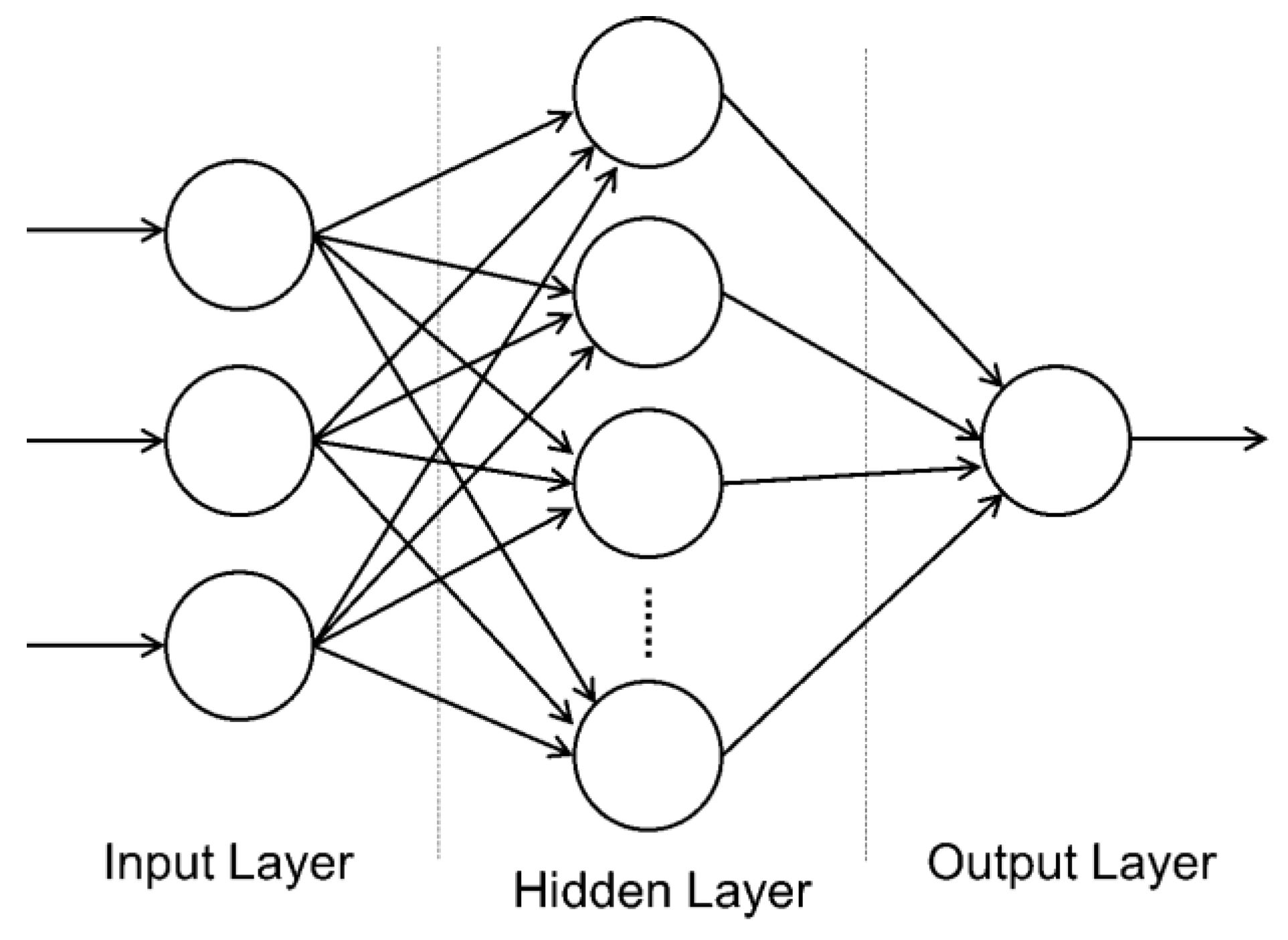
The Matlab Neural Network Tool was used to develop the DEM improvement scheme in this research. It provides a neural network to generalize nonlinear relationships between inputs and outputs using feed-forward and backpropagation networks. It contains multiple neurons arranged in layers, and all of these have connections. It consists of an input layer, one hidden layer, and one output layer; thus, the notation is a two-layer feedforward network, as shown in Figure 1 [42]. The training stage is able to converge with the optimal target function by means of the alteration in the weights systematically. Initially, random values are assigned to weights, and the network has to be trained to find the optimal weights. To achieve this, the first output of the neural network has to be compared to the desired output and an error is first determined; using this error, the weights of the network are adjusted proportionally to their contribution to the error in the output using the backpropagation algorithm [43,44].
In this study, the network is trained with the Levenberg–Marquardt (LM) backpropagation algorithm to minimize the error between the target and output layers using the mean squared error for the cost function [45,46]. Table 4 shows the input, target, and output layers in the ANN. In this study, the dataset of the training site was divided into 70% for training, 15% for an overfitting test, and 15% for independent testing of network performance. The selection of the data was conducted randomly. The Sentinel-2 reflectance values (bands 2–8A) and TanDEM-X were placed in the input layer and the ground truth elevations were placed in the target layer. Two separate ANN trainings were used, one only for buildings and the other for the entire area without buildings. Buildings were classified with building footprints from Open Street Map (OSM). The elevations of iTanDEM-X were the output of the resulting ANN process. The outputs from two ANNs were merged into one DEM using a mosaic to create a new raster function in ArcGIS [47]. In this study, the reported results originated from a neural network using only one hidden layer with a hyperbolic tangent activation function.
3.5. Flowchart of the Methodology
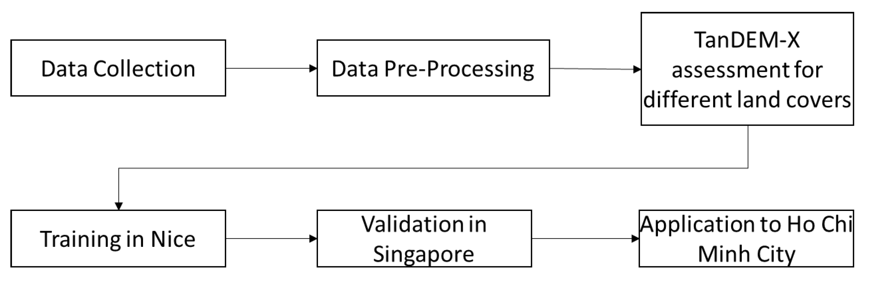
The methodology of this research is summarized in Figure 2. Various remote sensing data were collected, including satellite DEM and multispectral imagery. Then, the data were preprocessed to assess TanDEM-X’s accuracy and to prepare for ANN input. Finally, the data were trained in Nice, validated in Singapore, and applied to Ho Chi Minh City.
4. Assessment of TanDEM-X over Different Land Covers in Nice, France
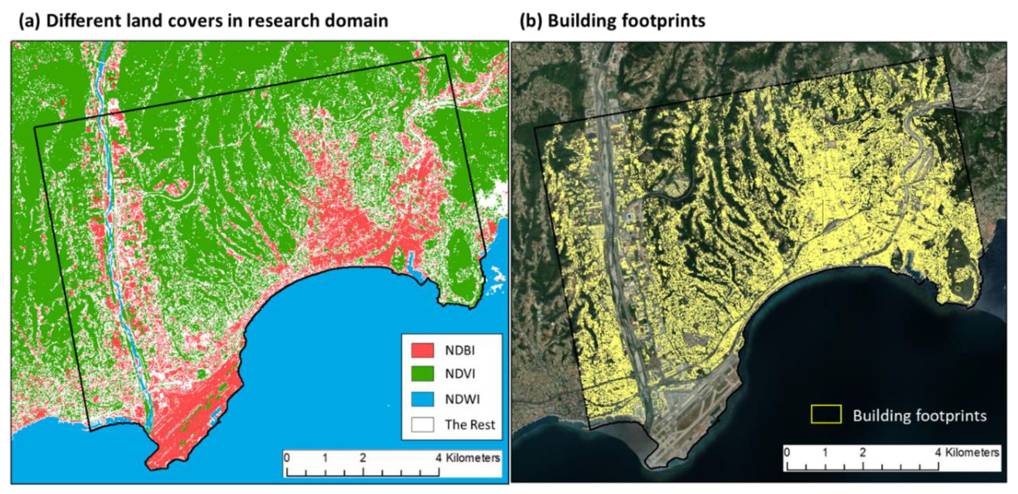
To better quantify the quality of TanDEM-X, elevation values were categorized by different land cover types. Three major land cover classes were considered—built-up area, vegetation, and water bodies—from the derived NDBI, NDVI, and NDWI, respectively. In addition, to separate the effect of open space in built-up areas, such as roads, airports, and stadiums from NDBI, pure building areas from building footprints were compared. Figure 3a shows three land covers, NDBI, NDVI, and NDWI, derived from Sentinel-2 in Nice. Figure 3b shows the building footprints provided by OSM. The area of the study domain was 74.3 km2 and its elevation ranged from 0 to 380 m.
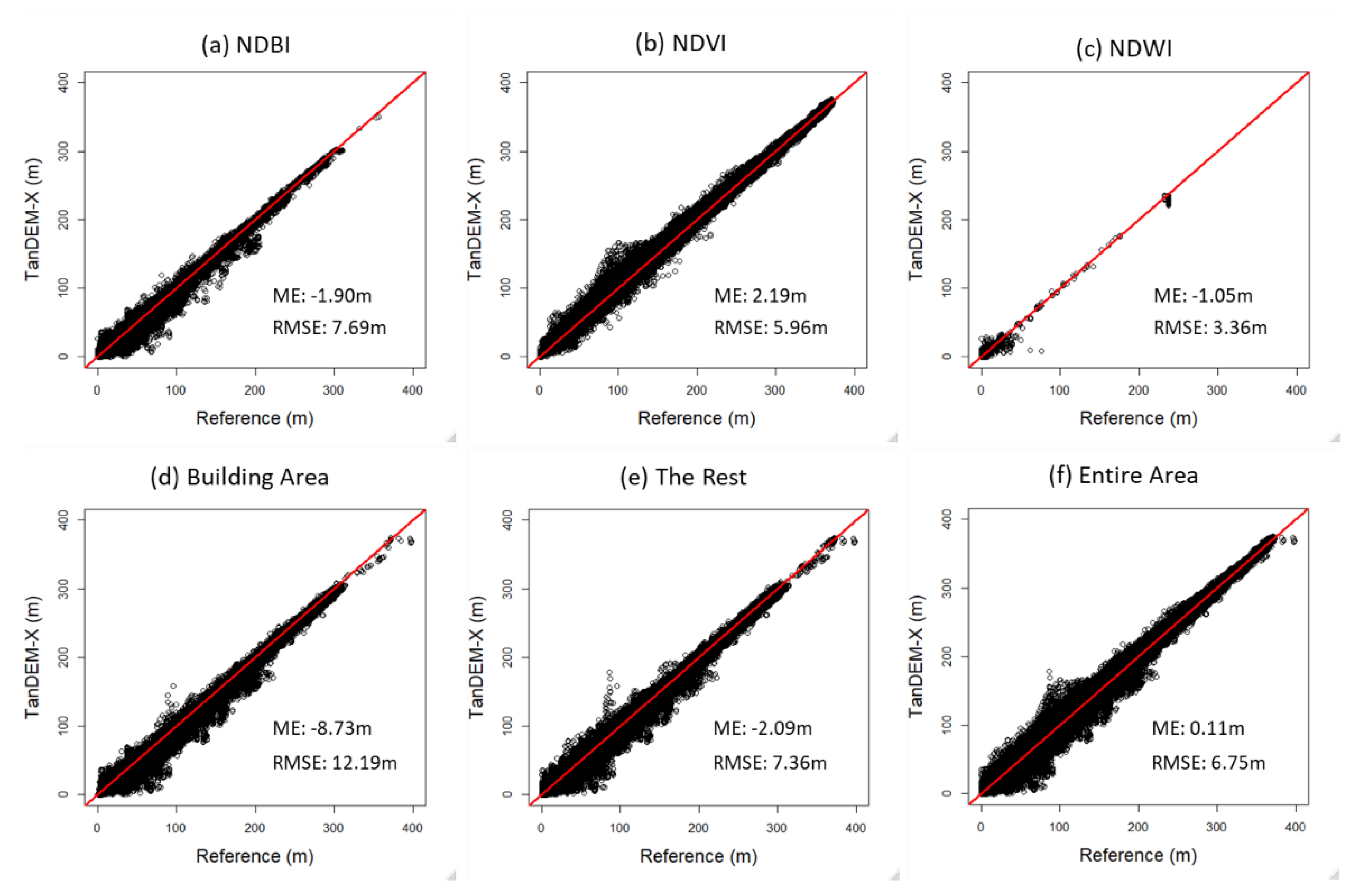
Figure 4 shows the scatterplot of TanDEM-X against the reference DEM for each land cover class. The performance of TanDEM-X over the NDBI area is shown in Figure 4a. The scatterplot and ME calculation show that TanDEM-X underestimated the elevation in the built-up area, with an RMSE of 7.69 m. Figure 4b shows the performance of TanDEM-X in the NDVI area. The calculated RMSE and ME were 5.96 m and 2.19 m, respectively. The scatterplot shows that TanDEM-X overestimated the vegetated area. Figure 4c–f shows the scatterplots with the ME and RMSE over NDWI, including buildings and the rest of the area (i.e., the area not classified in NDBI, NDVI, and NDWI).
Overall, there was a reasonable agreement between TanDEM-X and the reference DEM, with an RMSE of 6.75 m. The building area showed the greatest RMSE in different land cover areas, and the NDWI area showed the lowest RMSE of 3.36 m. Generally, TanDEM-X underestimated the elevations in built-up areas, buildings, and the rest of the area, while the elevations of vegetation areas were overestimated by TanDEM-X.
5. Performance of iTanDEM-X, Trained in Nice, When Applied in Singapore and Ho Chi Minh City (Vietnam)
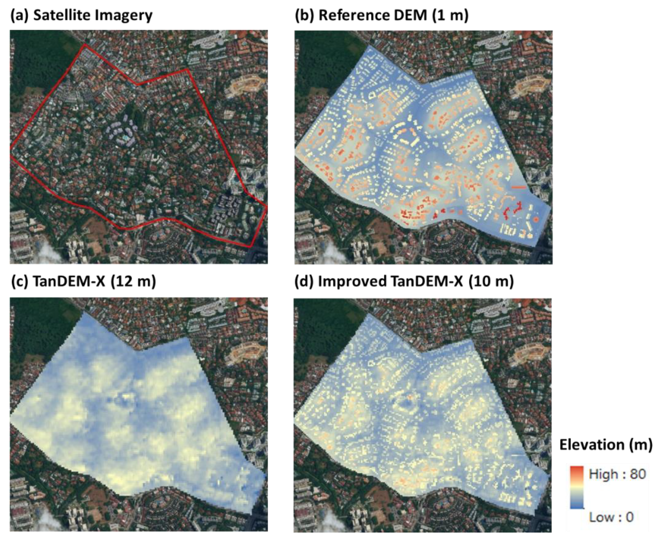
Kim et al. (2020) [4] showed that the ANN trained in Nice with SRTM_DEM (30 m resolution) could be applied to a faraway site, Singapore, to produce a DEM that is visually much clearer and with a much-reduced RMSE than the original SRTM_DEM. In this study, of greater interest is to see whether the ANN trained in Nice can generate a DEM in Singapore, with a significantly better quality than the original TanDEM-X. Note that Singapore has a high-resolution surveyed DEM (1 m resolution) for validation. To evaluate the performance of the iTanDEM-X in Singapore, elevations, classified by different land cover types, were assessed. Figure 5a shows the boundary of the study area in Singapore, while three DEM products, the reference DEM, TanDEM-X, and iTanDEM-X, are shown in Figure 5b–d, respectively. The reference DEM showed the clearest land shapes (i.e., buildings and roads), and iTanDEM-X captured the characteristics of the buildings much better than those of their counterparts in the original TanDEM-X.
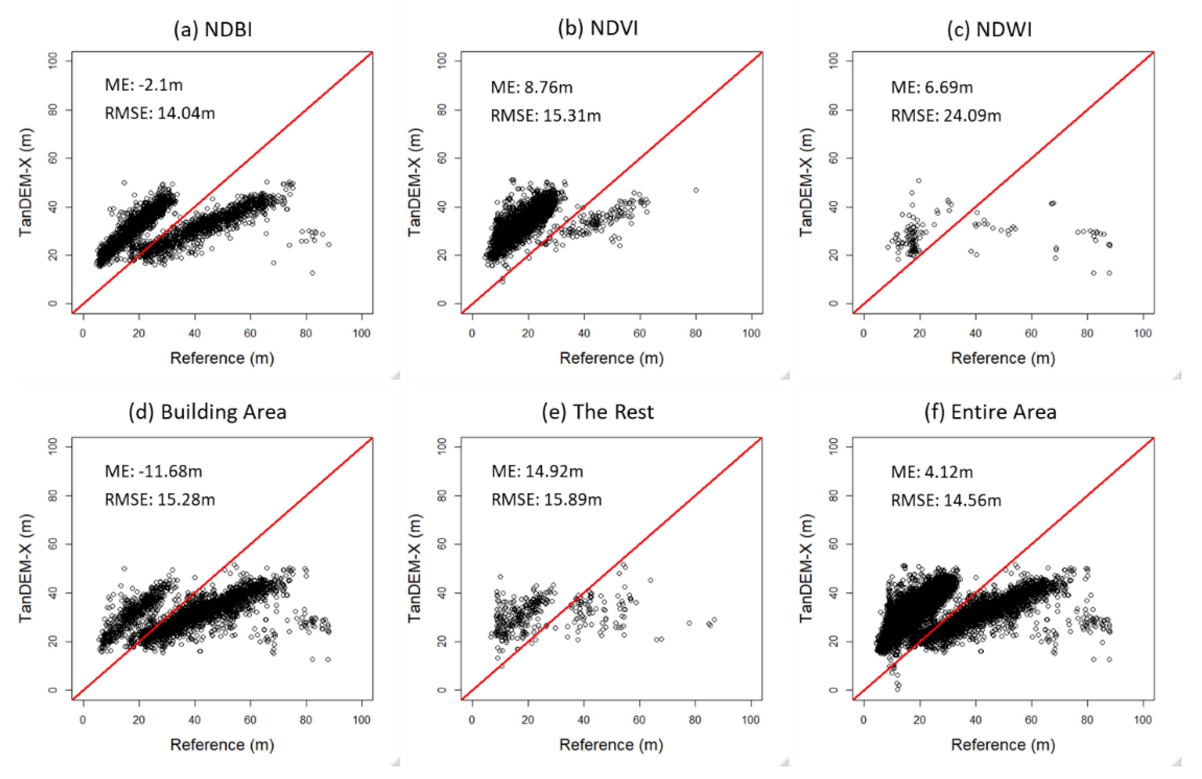
The scatterplots of TanDEM-X vs. the reference DEM are shown in Figure 6. Among the six scatterplots in Figure 6, NDVI and the building areas showed clear characteristics in the bias. The scatterplot of NDVI (Figure 6b) shows that the TanDEM-X values overestimated the elevation compared to the reference values, while the TanDEM-X values in the building area (Figure 6d) underestimated the elevation. This is a similar trend with the data from Nice. Overall, the RMSE value from the entire area was 14.56 m, and there were two clusters in the scatterplot, which reflected the overestimation in the vegetation area and underestimation in the building area.
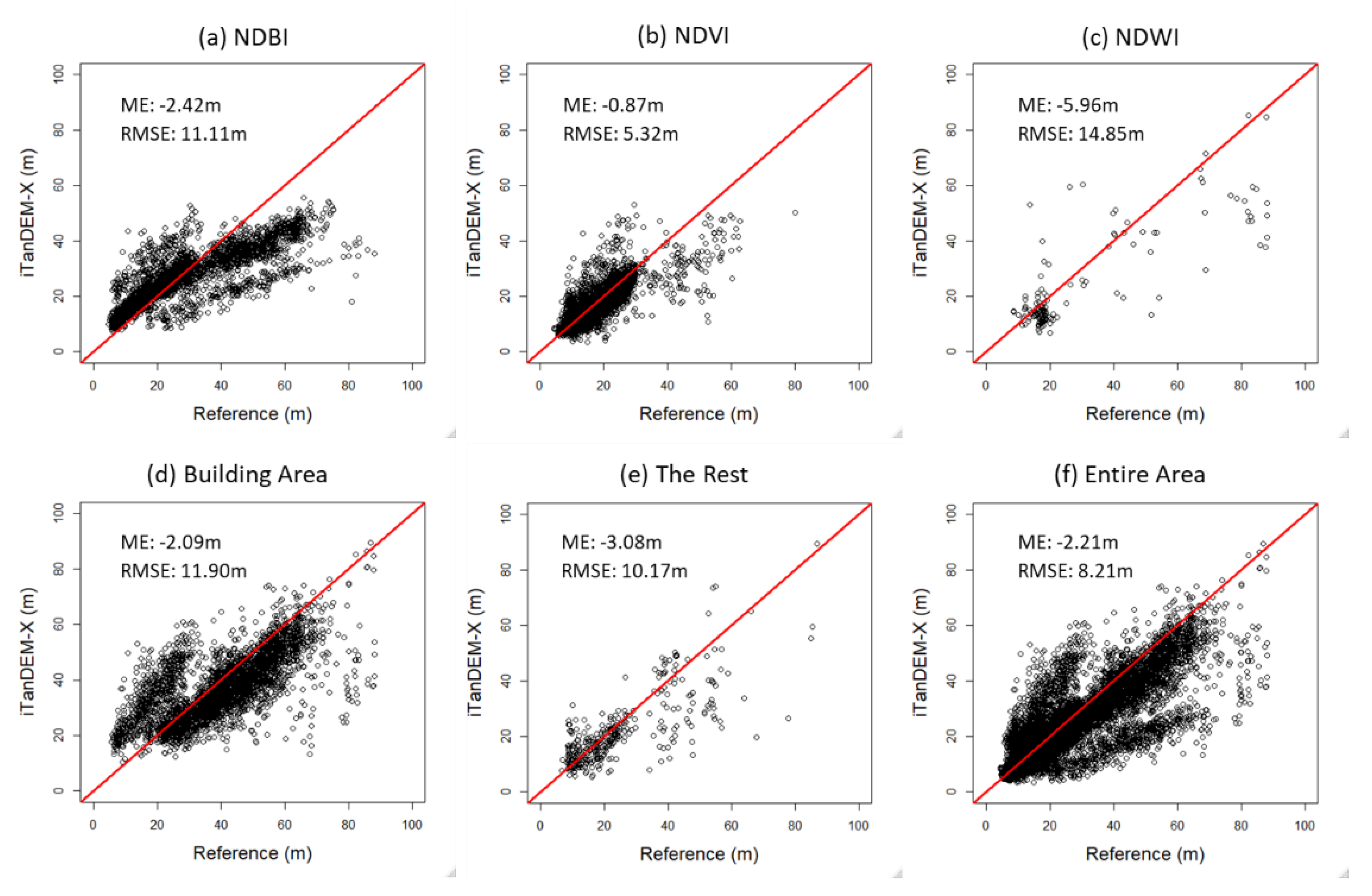
Figure 7 clearly demonstrates that the improved TanDEM-X had a better agreement with the reference DEM from all of the different land cover areas. In particular, the RMSE in NDVI was reduced from 15.31 to 5.32 m, which was a 65% improvement. The two clusters that were seen in the original TanDEM-X scatterplots had weakened outlines, and the points are placed at the centerline. As shown in Figure 7e, the RMSE was reduced from 14.56 to 8.21 m (a 43.6% reduction).
Table 5 summarizes the error statistics of TanDEM-X and iTanDEM-X compared to the reference DEM. The ME of the original TanDEM-X suggests that the error of the underestimated cluster contributed more weight than the overestimated cluster for built-up/building areas, while the overestimated cluster contributed more to vegetation areas. The error statistics demonstrated that iTanDEM-X significantly improved the overestimated vegetation areas of the original TanDEM-X.
The ANN trained in Nice was then applied to Ho Chi Minh City, where the ground truth DEM was not made available to the study team. The network performance, however, can use Google satellite imagery for visual comparison.
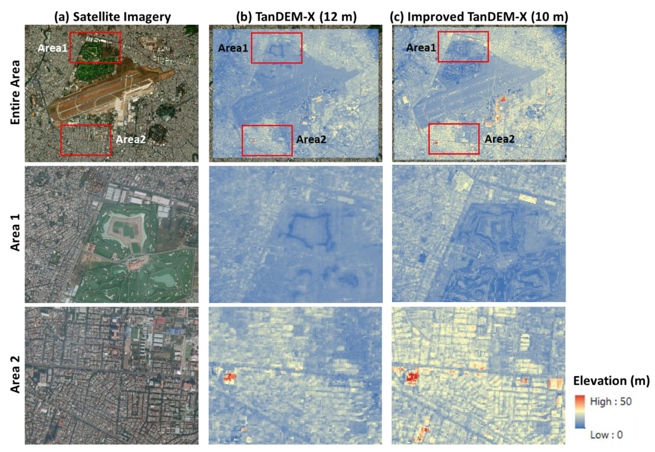
Figure 8 shows the satellite imagery and topography from TanDEM-X and iTanDEM-X near Tan Son Nhat International Airport in Ho Chi Minh City. Buildings, roads, and shapes of the grounds were much clearer in the iTanDEM-X. Two areas are highlighted for comparison; one area, Area 1, is mainly a vegetated area, while the other area, Area 2, is mainly a built-up area. In Area 1, the shapes of green patches and different land covers are clearly distinguished in iTanDEM-X. In Area 2, the roads and building blocks are clearly recognized, and matched well with the satellite imagery.
6. Discussion
The DEM improvement scheme was developed using an ANN with TanDEM-X, together with Sentinel-2 multispectral imagery. Firstly, the accuracy of TanDEM-X was assessed with ground truth data in Nice and Singapore over different land cover areas (NDBI, NDVI, and NDWI). These different land cover areas were derived from Sentinel-2 multispectral imagery, which exhibits different reflectance values for different wavelengths. In addition, the building footprints from OSM were used to distinguish the pure building areas. The areas that are not classified in the three land cover types above were expressed as the rest of the area. The different biases of the TanDEM-X elevations are observed in different land cover areas. The values are overestimated in the NDVI areas, clearly due to the X-band signal having little penetration into the vegetation cover [48]. On the contrary, TanDEM-X underestimates the elevation in NDBI and building areas; this is expected, as the NDBI value for a grid represents the average elevations of a low-lying area (or road) and high-rise buildings [49,50]. It is suggested to develop a method to set the threshold to complement the visual assessment with satellite imagery.
The trained ANN was able to classify the different land covers with the assistance of eight bands in Sentinel-2. Based on the various land characteristics, different weights were calculated to reduce the error between the elevation of TanDEM-X and the reference DEM. As summarized in Table 5, the performance of the iTanDEM-X showed a significant RMSE reduction of 43.6% over the entire area. The NDVI area showed the greatest improvement (65% reduction), while the NDBI area showed the least improvement (21% reduction). This can be explained by the fact that the building heights (higher than 60 m) did not clearly match with ground truth data (Figure 5), as the building heights in the Nice area are mostly less than 60 m, which is not as high as Singapore’s buildings [4].
Using more data from other remote sensing data sources (data fusion technique) should be considered to further improve the DEM scheme, as one sensor’s limitations could be compensated by another sensor’s strengths [26]. Additionally, different types of machine learning models should be investigated to assess the model performance for different land cover areas.
Therefore, it is necessary to pay more attention to use different deep learning methods, such as super-resolution based on a convolution neural network (CNN), together with various kind of geospatial and remote sensing data in future work.
7. Conclusions
This study demonstrated the robustness of a DEM improvement scheme, developed by Kim et al. [4], for a high-resolution satellite DEM (TanDEM-X, 12 m resolution). The artificial neural network was trained in Nice with a surveyed 1 m resolution DEM and then applied to two faraway sites, one with an equally high-resolution DEM in Singapore and another with no surveyed DEM in Ho Chi Minh City. The scheme used multispectral imagery and an ANN to reduce the error of the original TanDEM-X. The accuracy of TanDEM-X was first compared for different land covers in Nice and Singapore. Overall, the RMSE of TanDEM-X was assessed to be 6.75 and 14.56 m in Nice and Singapore, respectively. The error patterns were different over various land covers derived from NDBI, NDVI, and NDWI calculation and building footprints.
The ANN was trained in Nice with high-resolution ground truth data and validated in Singapore. The iTanDEM-X showed an over 43% RMSE reduction in the Singapore study domain. The degree of improvement, ranging from 21% to 65%, is different based on land covers. Upon completing the successful experiment, the ANN trained in Nice was then used with high confidence to improve TanDEM-X elsewhere, namely Ho Chi Minh City in this study. As no surveyed DEM of HCM City was made available to the team, only visual comparisons were conducted with Google satellite imagery. The iTanDEM-X showed much clearer land shapes (particularly roads and buildings) than its counterpart, the original TanDEM-X.
These results show promising, wide-ranging applications of a well-trained ANN, which, with a rich variety of patterns, can be very useful for developing countries, where a DEM is mostly not available/confidential or of low quality. In addition, one clear benefit of the developed scheme is that the trained ANN can be used to produce high-accuracy DEMs elsewhere quickly and at a relatively low cost.
Author Contributions
Conceptualization, D.E.K., S.-Y.L. and P.G.; Formal analysis, D.E.K. and J.L.; Funding acquisition, P.G. and G.S.; Investigation, S.-Y.L.; Methodology, D.E.K., J.L. and S.-Y.L.; Supervision, G.S.; Validation, D.E.K.; Visualization, D.E.K. and J.L.; Writing – original draft, D.E.K.; Writing – review & editing, J.L., S.-Y.L., P.G. and G.S. All authors have read and agreed to the published version of the manuscript.
Funding
This research received external funding from the National Research Foundation, Singapore, under its AI Singapore Programme (AISG Award No: AISG-100E/GC/RP/RPKS-2019-045).
Institutional Review Board Statement
Not applicable.
Informed Consent Statement
Not applicable.
Data Availability Statement
Not applicable.
Acknowledgments
This research is supported by the National Research Foundation, Singapore under its AI Singapore Programme (AISG Award No: AISG-100E/GC/RP/RPKS-2019-045). The contribution of DEM data from (1) Métropole Nice Côte d’Azur, (2) German Aerospace Center (DLR)—TanDEM-X, (3) Building and Construction Authority of Singapore are acknowledged.
Conflicts of Interest
The authors declare no conflict of interest.
References
- Liu, P.; Di, L.; Du, Q.; Wang, L. Remote Sensing Big Data: Theory, Methods and Applications. Remote Sens. 2018, 10, 711. [Google Scholar] [CrossRef] [Green Version]
- Huang, Y.; Chen, Z.-X.; Tao, Y.; Huang, X.-Z.; Gu, X.-F. Agricultural remote sensing big data: Management and applications. J. Integr. Agric. 2018, 17, 1915–1931. [Google Scholar] [CrossRef]
- Kalantar, B.; Ueda, N.; Saeidi, V.; Ahmadi, K.; Halin, A.A.; Shabani, F. Landslide Susceptibility Mapping: Machine and Ensemble Learning Based on Remote Sensing Big Data. Remote Sens. 2020, 12, 1737. [Google Scholar] [CrossRef]
- Kim, D.E.; Liong, S.-Y.; Gourbesville, P.; Andres, L.; Liu, J. Simple-Yet-Effective SRTM DEM Improvement Scheme for Dense Urban Cities Using ANN and Remote Sensing Data: Application to Flood Modeling. Water 2020, 12, 816. [Google Scholar] [CrossRef] [Green Version]
- Moudrý, V.; Lecours, V.; Gdulová, K.; Gábor, L.; Moudrá, L.; Kropáček, J.; Wild, J. On the use of global DEMs in ecological modelling and the accuracy of new bare-earth DEMs. Ecol. Model. 2018, 383, 3–9. [Google Scholar] [CrossRef]
- Favalli, M.; Fornaciai, A. Visualization and comparison of DEM-derived parameters. Application to volcanic areas. Geomorphology 2017, 290, 69–84. [Google Scholar] [CrossRef]
- Wang, D.; Kääb, A. Modeling glacier elevation change from DEM time series. Remote Sens. 2015, 7, 10117–10142. [Google Scholar] [CrossRef] [Green Version]
- Farr, T.G.; Rosen, P.A.; Caro, E.; Crippen, R.; Duren, R.; Hensley, S.; Kobrick, M.; Paller, M.; Rodriguez, E.; Roth, L. The shuttle radar topography mission. Rev. Geophys. 2007, 45. [Google Scholar] [CrossRef] [Green Version]
- Tachikawa, T.; Kaku, M.; Iwasaki, A.; Gesch, D.B.; Oimoen, M.J.; Zhang, Z.; Danielson, J.J.; Krieger, T.; Curtis, B.; Haase, J. ASTER Global Digital Elevation Model Version 2-Summary of Validation Results; NASA: Mountain View, CA, USA, 2011.
- Miliaresis, G.C.; Argialas, D. Segmentation of physiographic features from the global digital elevation model/GTOPO30. Comput. Geosci. 1999, 25, 715–728. [Google Scholar] [CrossRef]
- Florinsky, I.; Skrypitsyna, T.; Luschikova, O. Comparative accuracy of the AW3D30 DSM, ASTER GDEM, and SRTM1 DEM: A case study on the Zaoksky testing ground, Central European Russia. Remote Sens. Lett. 2018, 9, 706–714. [Google Scholar] [CrossRef]
- Wessel, B. TanDEM-X Ground Segment–DEM Products Specification Document; German Aerospace Center (DLR): Bonn, Germany, 2018.
- Krieger, G.; Zink, M.; Bachmann, M.; Bräutigam, B.; Schulze, D.; Martone, M.; Rizzoli, P.; Steinbrecher, U.; Antony, J.W.; De Zan, F. TanDEM-X: A radar interferometer with two formation-flying satellites. Acta Astronaut. 2013, 89, 83–98. [Google Scholar] [CrossRef] [Green Version]
- Wessel, B.; Huber, M.; Wohlfart, C.; Marschalk, U.; Kosmann, D.; Roth, A. Accuracy assessment of the global TanDEM-X Digital Elevation Model with GPS data. ISPRS J. Photogramm. Remote Sens. 2018, 139, 171–182. [Google Scholar] [CrossRef]
- Drusch, M.; Del Bello, U.; Carlier, S.; Colin, O.; Fernandez, V.; Gascon, F.; Hoersch, B.; Isola, C.; Laberinti, P.; Martimort, P. Sentinel-2: ESA’s optical high-resolution mission for GMES operational services. Remote Sens. Environ. 2012, 120, 25–36. [Google Scholar] [CrossRef]
- Roy, D.P.; Li, J.; Zhang, H.K.; Yan, L.; Huang, H.; Li, Z. Examination of Sentinel-2A multi-spectral instrument (MSI) reflectance anisotropy and the suitability of a general method to normalize MSI reflectance to nadir BRDF adjusted reflectance. Remote Sens. Environ. 2017, 199, 25–38. [Google Scholar] [CrossRef]
- Gatti, A.; Bertolini, A. Sentinel-2 Products Specification Document. 2018. Available online: https://earth.esa.int/documents/247904/685211/Sentinel-2+Products+Specification+Document (accessed on 15 March 2021).
- Andres, L.; Salas, W.A.; Skole, D. Fourier analysis of multi-temporal AVHRR data applied to a land cover classification. Remote Sens. 1994, 15, 1115–1121. [Google Scholar] [CrossRef]
- Ashish, D.; McClendon, R.W.; Hoogenboom, G. Land-use classification of multispectral aerial images using artificial neural networks. Int. J. Remote Sens. 2009, 30, 1989–2004. [Google Scholar] [CrossRef]
- Moody, D.I.; Brumby, S.P.; Rowland, J.C.; Altmann, G.L. Land Cover Classification in Multispectral Imagery Using Clustering of Sparse Approximations over Learned Feature Dictionaries; SPIE: Bellingham, WA, USA, 2014; Volume 8, pp. 1–19. [Google Scholar]
- Kim, D.; Sun, Y.; Wendi, D.; Jiang, Z.; Liong, S.-Y.; Gourbesville, P. Flood modelling framework for Kuching City, Malaysia: Overcoming the lack of data. In Advances in Hydroinformatics; Springer: Berlin, Germany, 2018; pp. 559–568. [Google Scholar]
- Gašparović, M.; Dobrinić, D.; Medak, D. Geometric accuracy improvement of WorldView-2 imagery using freely available DEM data. Photogramm. Rec. 2019, 34, 266–281. [Google Scholar] [CrossRef]
- Ravibabu, M.; Jain, K.; Singh, S.; Meeniga, N. Accuracy improvement of ASTER stereo satellite generated DEM using texture filter. Geo-Spat. Inf. Sci. 2010, 13, 257–262. [Google Scholar] [CrossRef]
- Wendi, D.; Liong, S.-Y.; Sun, Y.; Doan, C.D. An innovative approach to improve SRTM DEM using multispectral imagery and artificial neural network. J. Adv. Modeling Earth Syst. 2016, 8, 691–702. [Google Scholar] [CrossRef] [Green Version]
- Kim, D.-E.; Gourbesville, P.; Liong, S.-Y. Overcoming data scarcity in flood hazard assessment using remote sensing and artificial neural network. Smart Water 2019, 4, 2. [Google Scholar] [CrossRef]
- Muhadi, N.A.; Mohd Kassim, M.S.; Abdullah, A.F. Improvement of Digital Elevation Model (DEM) using data fusion technique for oil palm replanting phase. Int. J. Image Data Fusion 2019, 10, 232–243. [Google Scholar] [CrossRef]
- Meadows, M.; Wilson, M. A Comparison of Machine Learning Approaches to Improve Free Topography Data for Flood Modelling. Remote Sens. 2021, 13, 275. [Google Scholar] [CrossRef]
- Hajnsek, I.; Busche, T.; Schulze, D.; Buckreub, S.; Moreira, A. TanDEM-X: TanDEM-X Digital Elevation Models Announcement of Opportunity; TD-PD-AO-0033; German Aerospace Center (DLR): Bonn, Germany, 2016.
- Fan, H.; Zipf, A.; Fu, Q.; Neis, P. Quality assessment for building footprints data on OpenStreetMap. Int. J. Geogr. Inf. Sci. 2014, 28, 700–719. [Google Scholar] [CrossRef]
- Takagi, M. Accuracy of digital elevation model according to spatial resolution. Int. Arch. Photogramm. Remote Sens. 1998, 32, 613–617. [Google Scholar]
- Gruber, A.; Wessel, B.; Huber, M.; Roth, A. Operational TanDEM-X DEM calibration and first validation results. Photogramm. Eng. Remote Sens. 2012, 73, 39–49. [Google Scholar] [CrossRef]
- Lemoine, F.; Kenyon, S.; Factor, J.; Trimmer, R.; Pavlis, N.; Chinn, D.; Cox, C.; Klosko, S.; Luthcke, S.; Torrence, M. The Development of the Joint NASA GSFC and the National Imagery and Mapping Agency (NIMA) Geopotential Model EGM96; National Aeronautics and Space Administration, Goddard Space Flight Center: Greenbelt, MD, USA, 1998.
- Rouse, J.W.; Haas, R.H.; Deering, D.W.; Schell, J.A. Monitoring the Vernal Advancement and Retrogradation (Green Wave Effect) of Natural Vegetation; Remote Sensing Center, Texas A&M University: College Station, TX, USA, 1973. [Google Scholar]
- El-Gammal, M.; Ali, R.; Samra, R. NDVI threshold classification for detecting vegetation cover in Damietta governorate, Egypt. J. Am. Sci. 2014, 10, 2014. [Google Scholar]
- Kuc, G.; Chormański, J. Sentinel-2 imagery for mapping and monitoring imperviousness in urban areas. Int. Arch. Photogramm. Remote Sens. Spat. Inf. Sci. 2019, 42. [Google Scholar] [CrossRef] [Green Version]
- McFeeters, S.K. The use of the Normalized Difference Water Index (NDWI) in the delineation of open water features. Int. J. Remote Sens. 1996, 17, 1425–1432. [Google Scholar] [CrossRef]
- Du, Y.; Zhang, Y.; Ling, F.; Wang, Q.; Li, W.; Li, X. Water bodies’ mapping from Sentinel-2 imagery with modified normalized difference water index at 10-m spatial resolution produced by sharpening the SWIR band. Remote Sens. 2016, 8, 354. [Google Scholar] [CrossRef] [Green Version]
- Szypuła, B. Quality assessment of DEM derived from topographic maps for geomorphometric purposes. Open Geosci. 2019, 11, 843–865. [Google Scholar] [CrossRef]
- Sung, J.Y.; Lee, J.; Chung, I.-M.; Heo, J.-H. Hourly water level forecasting at tributary affected by main river condition. Water 2017, 9, 644. [Google Scholar] [CrossRef] [Green Version]
- Li, Z. On the measure of digital terrain model accuracy. Photogramm. Rec. 1988, 12, 873–877. [Google Scholar] [CrossRef]
- Ioannou, K.; Myronidis, D.; Lefakis, P.; Stathis, D. The use of artificial neural networks(anns) for the forecast of precipitation levels of lake doirani(N. greece). Fresenius Environ. Bull. 2010, 19, 1921–1927. [Google Scholar]
- Haykin, S. Neural Networks: A Comprehensive Foundation; Prentice Hall PTR: Hoboken, NJ, USA, 1994; p. 768. [Google Scholar]
- Rosenblatt, F. Principles of Neurodynamics. Perceptrons and the Theory of Brain Mechanisms; VG-1196-G-8; Cornell Aeronautical Lab Inc.: Buffalo, NY, USA, 1961. [Google Scholar]
- Widrow, B.; Hoff, M.E. Associative Storage and Retrieval of Digital Information in Networks of Adaptive “Neurons”. In Biological Prototypes and Synthetic Systems: Volume 1 Proceedings of the Second Annual Bionics Symposium sponsored by Cornell University and the General Electric Company, Advanced Electronics Center, Ithaca, NY, USA, 30 August–1 September 1961; Bernard, E.E., Kare, M.R., Eds.; Springer: Boston, MA, USA, 1962; p. 160. [Google Scholar] [CrossRef]
- Levenberg, K. A Method for the Solution of Certain Non-Linear Problems in Least Squares. Q. Appl. Math. 1944, 2, 164–168. [Google Scholar] [CrossRef] [Green Version]
- Marquardt, D.W. An Algorithm for Least-Squares Estimation of Nonlinear Parameters. J. Soc. Ind. Appl. Math. 1963, 11, 431–441. [Google Scholar] [CrossRef]
- ESRI. ArcGIS Desktop 10.5, Environmental Systems Research Institute, Release 10.5. 2018. Available online: https://desktop.arcgis.com (accessed on 15 March 2021).
- Meyer, F. Spaceborne Synthetic Aperture Radar: Principles, data access, and basic processing techniques. In Synthetic Aperture Radar (SAR) Handbook: Comprehensive Methodologies for Forest Monitoring and Biomass Estimation; NASA: Washington, DC, USA, 2019; pp. 21–64. Available online: https://servirglobal.net/Global/Articles/Article/2674/sar-handbook-comprehensive-methodologies-for-forest-monitoring-and-biomass-estimation (accessed on 15 March 2021).
- Hawker, L.; Bates, P.; Neal, J.; Rougier, J. Perspectives on Digital Elevation Model (DEM) Simulation for Flood Modeling in the Absence of a High-Accuracy Open Access Global DEM. Front. Earth Sci. 2018, 6. [Google Scholar] [CrossRef] [Green Version]
- Zhang, K.; Gann, D.; Ross, M.; Biswas, H.; Li, Y.; Rhome, J. Comparison of TanDEM-X DEM with LiDAR data for accuracy assessment in a coastal urban area. Remote Sens. 2019, 11, 876. [Google Scholar] [CrossRef] [Green Version]
Figure 1.
Schematic diagram of a two-layer feedforward network.

Figure 2.
Flowchart of the methodology.

Figure 3.
Different land covers derived from Sentinel-2 and the building footprint in Nice, France: (a) Different land covers, (b) Building footprints.
Figure 3.
Different land covers derived from Sentinel-2 and the building footprint in Nice, France: (a) Different land covers, (b) Building footprints.

Figure 4.
Scatterplots with ME and RMSE comparison of TanDEM-X over different land covers in Nice, France: (a) NDBI, (b) NDVI, (c) NDWI, (d) Building Area, (e) The Rest, (f) The Entire Area.
Figure 4.
Scatterplots with ME and RMSE comparison of TanDEM-X over different land covers in Nice, France: (a) NDBI, (b) NDVI, (c) NDWI, (d) Building Area, (e) The Rest, (f) The Entire Area.

Figure 5.
Visual assessment of TanDEM-X and iTanDEM-X of the urban area in Singapore: (a) Satellite Imagery, (b) Reference DEM (1 m), (c) TanDEM-X (12 m), (d) improved TanDEM-X (10 m).
Figure 5.
Visual assessment of TanDEM-X and iTanDEM-X of the urban area in Singapore: (a) Satellite Imagery, (b) Reference DEM (1 m), (c) TanDEM-X (12 m), (d) improved TanDEM-X (10 m).

Figure 6.
Scatterplots of TanDEM-X vs. the reference DEM and performance measures ME and RMSE: different land covers in Singapore: (a) NDBI, (b) NDVI, (c) NDWI, (d) Building Area, (e) The Rest, (f) The Entire Area.
Figure 6.
Scatterplots of TanDEM-X vs. the reference DEM and performance measures ME and RMSE: different land covers in Singapore: (a) NDBI, (b) NDVI, (c) NDWI, (d) Building Area, (e) The Rest, (f) The Entire Area.

Figure 7.
Scatterplots of iTanDEM-X vs. reference DEM and performance measures ME and RMSE: different land covers in Singapore: (a) NDBI, (b) NDVI, (c) NDWI, (d) Building Area, (e) The Rest, (f) The Entire Area.
Figure 7.
Scatterplots of iTanDEM-X vs. reference DEM and performance measures ME and RMSE: different land covers in Singapore: (a) NDBI, (b) NDVI, (c) NDWI, (d) Building Area, (e) The Rest, (f) The Entire Area.

Figure 8.
Visual assessment of iTanDEM-X in Ho Chi Minh City, Vietnam: (a) Satellite Imagery, (b)TanDEM-X (12 m), (c) improved TanDEM (10 m).
Figure 8.
Visual assessment of iTanDEM-X in Ho Chi Minh City, Vietnam: (a) Satellite Imagery, (b)TanDEM-X (12 m), (c) improved TanDEM (10 m).


Table 1.
Primary objective of the TanDEM-X mission [13].
Table 1.
Primary objective of the TanDEM-X mission [13].
| Parameter | Specification | Requirement |
|---|---|---|
| Relative vertical accuracy | 90% linear point to point error in 1° cell | 2 m (slope < 20%) 4 m (slope > 20%) |
| Absolute vertical accuracy | 90% linear error | 10 m |
| Spatial resolution | Independent pixels | 12 m (0.4 arcseconds) |
Table 2.
Property of collected Sentinel-2 multispectral imagery.
| Property | Nice, France | Singapore | Ho Chi Minh City, Vietnam |
|---|---|---|---|
| Entity ID | L1C_T32TLP_A016836_20180912T103308 | L1C_T48NUG_A004863_20180210T033204 | L1C_T48PXS_A010583_20190317T033028 |
| Acquisition Date | 12 September 2018 | 10 February 2018 | 17 March 2019 |
| Tile Number | T32TLP | T48NUG | T48NUG |
| Cloud Cover (%) | 1.5258 | 5.6381 | 1.0181 |
| Platform | SENTINEL-2A | SENTINEL-2B | SENTINEL-2B |
| Processing Level | LEVEL-1C | LEVEL-1C | LEVEL-1C |
Table 3.
The formula of the land cover index and the value of the threshold used in this research.
| Land Cover Index | Formula in Sentinel-2 | The Range of the Values and Threshold | |
|---|---|---|---|
| Nice, France | Singapore | ||
| NDVI | −0.77–1; >0.3 | −0.23 to 0.72; >0.4 | |
| NDBI | −1–0.69; >0.05 | −0.59–0.41; >0.05 | |
| NDWI | −1–0.77; >0.03 | −0.47–0.43; >0 | |
Table 4.
Input variable, target, and output layers in ANN training.
| Input Variable | Target Layer | Output Layer |
|---|---|---|
| Reflectance values of Sentinel-2, multispectral imagery (Band 2–8A) TanDEM-X elevations | Ground truth | Improved (Rectified) TanDEM-X |
Table 5.
The error patterns of TanDEM-X and iTanDEM-X for different land covers in Singapore.
| Land Covers | TanDEM-X | iTanDEM-X | ||
|---|---|---|---|---|
| ME (m) | RMSE (m) | ME (m) | RMSE (m) | |
| NDBI | −2.10 | 14.04 | −2.42 | 11.11 |
| NDVI | 8.76 | 15.31 | −0.87 | 5.32 |
| NDWI | 6.69 | 24.09 | −5.96 | 14.85 |
| Building Area | −11.68 | 15.28 | −2.09 | 11.90 |
| The Rest | 14.92 | 15.89 | −3.08 | 10.17 |
| Entire Area | 4.12 | 14.56 | −2.21 | 8.21 |
Publisher’s Note: MDPI stays neutral with regard to jurisdictional claims in published maps and institutional affiliations. |
© 2021 by the authors. Licensee MDPI, Basel, Switzerland. This article is an open access article distributed under the terms and conditions of the Creative Commons Attribution (CC BY) license (https://creativecommons.org/licenses/by/4.0/).
Share and Cite
MDPI and ACS Style
Kim, D.E.; Liu, J.; Liong, S.-Y.; Gourbesville, P.; Strunz, G. Satellite DEM Improvement Using Multispectral Imagery and an Artificial Neural Network. Water 2021, 13, 1551. https://doi.org/10.3390/w13111551
AMA Style
Kim DE, Liu J, Liong S-Y, Gourbesville P, Strunz G. Satellite DEM Improvement Using Multispectral Imagery and an Artificial Neural Network. Water. 2021; 13(11):1551. https://doi.org/10.3390/w13111551
Chicago/Turabian StyleKim, Dong Eon, Jiandong Liu, Shie-Yui Liong, Philippe Gourbesville, and Günter Strunz. 2021. "Satellite DEM Improvement Using Multispectral Imagery and an Artificial Neural Network" Water 13, no. 11: 1551. https://doi.org/10.3390/w13111551
Note that from the first issue of 2016, this journal uses article numbers instead of page numbers. See further details here.