Article

Assessing the Use of Dual-Drainage Modeling to Determine the Effects of Green Stormwater Infrastructure on Roadway Flooding and Traffic Performance

1
Department of Civil and Environmental Engineering, Colorado State University, Fort Collins, CO 80523, USA
2
Wright Water Engineers, Denver, CO 80211, USA
*
Author to whom correspondence should be addressed.
Water 2021, 13(11), 1563; https://doi.org/10.3390/w13111563
Submission received: 16 April 2021 / Revised: 20 May 2021 / Accepted: 26 May 2021 / Published: 31 May 2021

Abstract

:
Green stormwater infrastructure (GSI) is increasingly used to reduce stormwater input to the subsurface stormwater network. This work investigated how GSI interacts with surface runoff and stormwater structures to affect the spatial extent and distribution of roadway flooding and subsequent effects on the performance of the traffic system using a dual-drainage model. The model simulated roadway flooding using PCSWMM (Personal Computer Stormwater Management Model) in Harvard Gulch, Denver, Colorado, and was then used in a microscopic traffic simulation using the Simulation of Urban Mobility Model (SUMO). We examined the effect of converting between 1% and 5% of directly connected impervious area (DCIA) to bioretention GSI on roadway flooding. The results showed that even for 1% of DCIA converted to GSI, the extent and mean depth of roadway flooding was reduced. Increasing GSI conversion further reduced roadway flooding depth and extent, although with diminishing returns per additional percentage of DCIA converted to GSI. Reduced roadway flooding led to increased average vehicle speeds and decreased percentage of roads impacted by flooding and total travel time. We found diminishing returns in the roadway flooding reduction per additional percentage of DCIA converted to GSI. Future work will be conducted to reduce the main limitations of insufficient data for model validation. Detailed dual-drainage modeling has the potential to better predict what GSI strategies will mitigate roadway flooding.

1. Introduction

The increase in impervious surfaces characteristic of urbanization leads to higher peak runoff and total runoff volume in receiving water bodies [1]. These effects of urbanization indicate a loss of the watershed’s ability to naturally mitigate flooding and must be compensated for by the implementation of stormwater management practices [2]. These stormwater management practices are commonly inadequately sized, designed, or maintained to mitigate the frequency and magnitude of floods in urban watersheds [3,4]. Climate change has increased and will likely continue to increase the magnitude, intensity, and frequency of precipitation events, further straining stormwater systems [5].
Urban flooding results in repeated damage to property and infrastructure, economic disruption, and increased risk to human health and safety [6,7]. Assessment of urban flood impacts is challenging as flood events are often highly localized, may occur outside of FEMA (Federal Emergency Management Agency)-designated floodplains, and are often not large enough to trigger public reports to local municipalities. Survey data from across the United States found that urban flooding outside of established floodplains is common and urban flooding disproportionately affects lower-income communities [6].
The frequent disruption caused by small events of roadway flooding, called nuisance flooding, hides the cumulative impact roadway flooding has on communities and transportation systems [8]. Roadway flooding leads to the disruption of transportation systems even when flood depths are still passable by causing hazardous driving conditions that require a reduced safe driving speed. Because of the connectivity of traffic networks, localized roadway flooding can cause traffic disruptions that reach far beyond the extent of the flooding [9]. These disruptions can cause significant economic loss [7,8] and pose a risk to the function of transportation networks during emergency events [9].
The impact of flooding on transportation has attracted increasing attention in recent years. A flooding-transportation interaction analysis includes flooding analysis, providing the flood depth on roads, and traffic analysis, examining the performance of the disrupted road network. A dynamic flooding-transportation framework showed that because of knock-on effects, the performance of non-flooded roads could be impacted indirectly [10]. Increasing urban flooding may lead to nonlinearly increasing disruptions of traffic performance [11,12].
Previous research [13] used microscopic traffic flow simulations to assess the accident vulnerability of vehicles during hazardous driving conditions. Our work used microscopic traffic flow simulations to examine the specific hazard of roadway flooding and the effects of flooding on traffic performance. Avoiding a binary view of flooded roadways, assumed to be either fully blocked or open with free-flow traffic, a more realistic disruption status of roadways due to flooding can be evaluated by using a floodwater depth-disruption function. Depth-disruption functions [11] describe the relationship between floodwater depth and vehicle speed and have been developed with quantitative data from experiments, simulations, and observations. Therefore the level of disruption from flooding depends directly on roadway flooding depth during storm events.
One possible strategy to mitigate roadway flooding is the implementation of green stormwater infrastructure (GSI). GSI are types of stormwater control measures (SCMs) that use infiltration or harvest to reduce the amount of water directly entering the subsurface stormwater network [4,14]. The effect of a single structure or small-scale GSI networks has been widely studied, and it has been shown that, depending on the design, infiltration, and rainfall conditions, GSI can reduce and delay the peak runoff entering into the stormwater network [14,15]. At a watershed scale, infiltration and harvest-based GSI generally increase runoff thresholds and decrease peak flow and volume [16]. Less consensus has been established on how much impervious area needs to be converted to GSI to see reductions in peak flow and volume [17], or where in the watershed, it is optimal to apply GSI. One study determined that 10–15% of total impervious area needed to be converted to GSI to see a reduction in neighborhood-scale flooding and 20% conversion to significantly reduce roadway flooding, after which more conversion had diminishing marginal benefit [4].
Distributed models, such as the EPA stormwater management model (SWMM), are often used for detailed site-scale or simplified watershed-scale stormwater models, but less often for a detailed watershed-scale because of the laborious model setup procedures and high data requirements [18]. Because of these modeling limitations, the current understanding of how individual GSI units interact with surface runoff, flooding, stormwater networks, and neighboring GSI is unclear. Previous studies examining GSI impacts on urban flooding utilized a simplified stormwater network and examined flood volume at specific locations within the stormwater network, also called nodes [15], or in a small-scale (0.313 km2) stormwater network using a combined index based on the flooded volume, rate, and duration at network nodes [19]. However, this previous work examining GSI impacts on urban flooding did not model urban flooding as a 2D water surface, which limits the physical understanding of how GSI affects urban systems, such as transportation networks, beyond the generalized metric of flood reduction at nodes.
An alternative method to examining node-based flooding to capture the interaction between GSI, surface runoff, and stormwater networks is utilizing dual-drainage modeling. Dual-drainage modeling couples a 2D surface runoff model domain and 1D subsurface stormwater network model domain and has bidirectional flow between the two modeling domains [7,20,21]. Because of the computational demand required to model bidirectional interaction of distributed 2D surface runoff and 1D stormwater drainage systems for larger study areas, the conceptual understanding of dual-drainage modeling has long outpaced the ability to execute such models. Observations of surcharge from stormwater inlets or flood depths are sparse, and even as computational advances make complex dual-drainage models more accessible, the lack of observed data for comparison is a critical limitation [22]. A potential solution to a lack of calibration data for urban flooding is the use of resident reports of flooding [23]. The use of dual-drainage modeling to simulate flooding caused by exceedance of the subsurface stormwater system capacity across the entire study area to represent urban roadway flooding allowed us to address the following research questions:
  • How can dual-drainage modeling help determine the effect of GSI networks on the depth, flooded extent, and spatial distribution of roadway flooding?
  • How do GSI networks affect the performance of the traffic system during a storm event?
  • What are the limitations of dual-drainage modeling for characterizing the effects of GSI networks on roadway flooding?

2. Materials and Methods

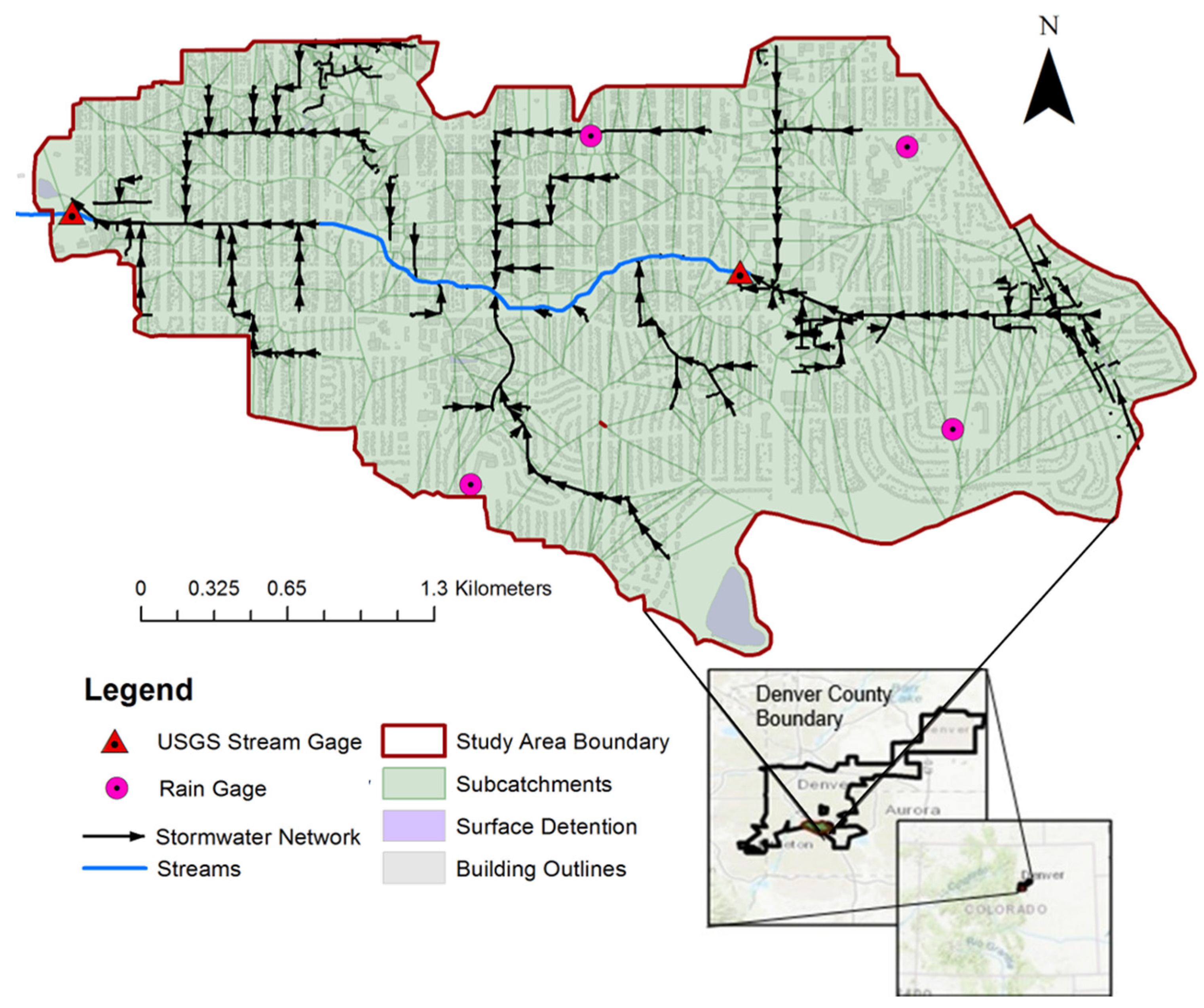
2.1. Study Area and Data Sources

The study area is a sub-basin of the Harvard Gulch watershed located in Denver, CO, USA, bordering Englewood, Colorado (Figure 1). This region of Colorado just east of the Rocky Mountains is characterized as a semi-arid climate and receives an average of 381 mm of precipitation per year [24]. Harvard Gulch was categorized as a medium to high priority basin for green infrastructure planning and improvements in a Denver Public Works report [25]. Harvard Gulch flows east to west through the watershed, with sections of naturalized open channel, concrete trapezoidal channel, and box culverts. There are two US Geological Survey (USGS) stream gages located within the study area: the upstream gage 06711570 is located at Colorado Boulevard, and the downstream gage 06711575 is located at Harvard Gulch Park near the western edge of the study area and is also referred to here as the outfall. Harvard Gulch has also been used as a study watershed for precipitation analysis [26].
In 2016, the Matrix Design group (Denver, CO, USA) produced a conceptual design report for the Harvard Gulch and Dry Gulch Major Drainageway Plan, including hydrological modeling using EPA SWMM (version 5.0.22, United States Environmental Protection Agency, Washington, DC, USA) and hydraulic modeling with HEC-RAS (version 4.1.0, United States Army Corps of Engineers, Davis, CA, USA) and FLO-2D (Flo 2D software, Inc. Nutrioso, AZ, USA) to examine the hydrologic and streamflow response to rainfall of specific return periods [27]. Information from the report was used to verify input data used to develop the stormwater model for this project, including drainage area delineations, storage curves, soil classification, flood frequency analysis, and channel geometry, as well as useful background on stormwater management in the study area. However, the previously developed model could not be directly used for the purposes of this study as it did not describe structure-scale details of the stormwater network and interactions with overland flow. Additionally, in order to isolate the runoff and stormwater network draining to the USGS gage 06711575 at Harvard Gulch Park, the study area outfall where calibration will be performed (Figure 1), the study area of this project covers a subset (43.4%) of the area assessed by Matrix Design Group in 2016. The resulting catchment area is 8.26 km2, has an average imperviousness of 36%, and an average slope of 0.44%. The directly connected impervious area (DCIA) [1] was estimated as 45% of the impervious area, or 16.2% of the catchment area, using a Denver-specific equation [28]. Harvard Gulch is considered a fully developed watershed, with mainly single and multi-family residential land use, along with some park and public spaces and commercial land use [29]. Imperviousness and land use data were collected from the City and County of Denver Open Data Catalog [29] and were most recently updated in 2016. The average slope was computed from the 3 m resolution digital elevation model (DEM) from the National Elevation Dataset. There is no soil classification by the United States Department of Agriculture (USDA) Natural Resources Conservation Survey (NRCS) Web Soil Survey available for the study area. However, the adjacent neighborhood in Englewood, Colorado, has a soil classification of type C, which was used as an approximate soil classification for the study area [30]. There are five USGS rain gages located within the study area (Figure 1), with rainfall measured at 5 min intervals.

2.2. Stormwater Model Application

In order to model the interactions between overland flow (2D system) and the subsurface stormwater network (1D system), a dual-drainage model with major and minor system domains was developed in PCSWMM (Personal Computer Stormwater Management Model, EPA Stormwater Management Model for PC, Version 7.2.2785, CHI, Guelph, Ontario, Canada) [31].

2.2.1. 1D Minor System Application

The minor system is comprised of stormwater network data acquired from the City and County of Denver Open Data Catalog (https://www.denvergov.org/opendata, accessed on 1 June 2019), including conduits, inlets, manholes, and underground storage as ArcGIS (version 10.5.1, ESRI, Vienna, VA, USA) shapefiles. The stormwater network, separate from the wastewater network, drains to Harvard Gulch at multiple outlet locations distributed along the stream channel within the study area.
The open channel of Harvard Gulch was represented as a component of the minor system using irregular and open-trapezoid cross-sections. There are 27 bridge crossings of the Harvard Gulch channel within the study area; representation of the open channel as minor system conduits made it possible to easily represent the channel passing below the bridge decks [27]. The irregular channel cross-sections were determined using the transect tool in PCSWMM with the 1 m DEM from the National Elevation Dataset (https://ned.usgs.gov, accessed on 1 December 2019), resulting in 46 transects along the irregular channel. The trapezoidal channel was considered to be uniform with a maximum depth of 2.74 m, bottom width of 2.44 m, and top width of 9.75 m [27]. Channel slopes were approximated from attributes of the conduits representing Harvard Gulch in the City and County of Denver stormwater data. Dry weather flows were computed from the streamflow recorded during the week prior to the simulation storm event on 24 June 2015, during which no precipitation was recorded at the upstream USGS gage 06711570. The average of these flows was applied as a constant inflow of 0.072 m3/s at the closest irregular channel node to the upstream gage in all simulations. The outfall of the minor system was assigned at the downstream USGS gage 06711575.
Subcatchments were delineated using the Voronoi decomposition tool in PCSWMM to create Theissen polygons based on the location of inlets in the watershed, resulting in 513 subcatchments [32]. The average slope and percent imperviousness of the subcatchments were computed from the 3 m DEM from the National Elevation Dataset to reduce local changes in elevation in the 1 m DEM, and percent imperviousness was computed using the most recent impervious area data (2016) from the City and County of Denver, respectively (Table 1). The outlet of the subcatchments was assigned to be the lowest elevation 2D node (described below) adjacent to the minor system inlet used for subcatchment delineation. The assignment of the subcatchment outlet to a 2D node is recommended for modeling overland flow entering the minor system via inlets and to represent rainfall-induced flooding. The rain gages located within the study area were assigned to subcatchments using Theissen polygons. The modified Green Ampt method was used to represent infiltration based on the soil classification of type C soil (Table 1).

2.2.2. Stormwater Network Data Completeness

Stormwater network data were gathered from the City and County of Denver. Missing data were approximated using a variety of methods, which are described in detail in Appendix A. There are only three underground storage nodes within the study area, two of which are underground detention pipes that were modeled using connected conduits and nodes. The third storage node was modeled as a rectangular detention vault with geometry determined from the area of the node feature in GIS and the depth attribute. Because of the degree of missing or incomplete data available for the geometry of surface storage facilities within the study area, it was assumed that the surface storage is best represented in the major system model by the topographical depressions in the DEM used to develop the major system model domain.

2.2.3. 2D Major System Application

The 2D major system utilizes the same SWMM5 engine as in the 1D minor system to model overland flow by creating a mesh of links and nodes representing the surface of the study area. The depth of water is measured in the nodes, and dynamic wave routing is used to allow flow in connecting links, which are represented as wall-less rectangular conduits with a width of the designated cell resolution. Input layers for the 2D major system application include road centerlines and widths, 1 m DEM, and building outlines. All data sources were acquired from the City and County of Denver Open Data Catalog, apart from the 1 m and 3 m DEM, which were acquired from the National Elevation Dataset. To produce the 2D mesh, the study area was broken into separate bounding areas for roads and surrounding areas. The total area delineated as roads were 0.70 km2 and the surrounding area was 7.56 km2. The resulting 2D major system model consists of 125,420 nodes and 313,054 conduits that delineate 126,153 2D cells. The 2016 building outline data from the City and County of Denver open data catalog was used as the obstructions layer, which excludes buildings from the 2D mesh.

2.2.4. Minor and Major System Connection

Interactions between the major and minor system domains occur primarily at catchbasin inlet and outlet nodes. There are six known types of inlets within the study area that are described in the Transportation Standards and Details from the City and County of Denver Public Works Department that fall into three general categories: curb opening, grated, and combination. Inlets can be installed as multi-inlets with multiple openings in series capturing runoff at a single location [34]. When runoff exceeds the inlet capacity, or debris reduces the inlet capacity, runoff may pond around, pass over, or, in more extreme cases, flow out of the inlet. Runoff re-enters the major system through outlets, most often conveying water into surface storage such as an extended detention basin or into a stream channel. In more extreme storm events, the interaction between the major and minor systems can also occur due to surcharged manholes where the pressure of water in the manhole is great enough to lift the manhole cover and flow out of the minor system.
In PCSWMM, nodes in the minor system that represent inlets are connected to the major system nodes via outlets, which allows for bi-directional flow. Each connecting outlet was assigned a rating curve from City and County of Denver Storm Drainage Design and Technical Criteria based on the inlet type relating elevation head above the inlet to flow. There were 397 inlets within the study of an unknown type, and these were assigned an average rating curve [35]. Minor system outlets to Harvard Gulch and surface storage facilities, as well as the open channel conduits, were connected to the major system with direct connections that co-locate the nearest major and minor system nodes.

2.3. Stormwater Simulations

The model was calibrated using the Sensitivity-based Radio Tuning Calibration (SRTC) tool in PCSWMM. The SRTC tool varies parameters based on the parameter uncertainty (Table 1) [36]. Sensitivity analysis and calibration using the SRTC tool were performed for seven parameters: impervious Manning’s roughness coefficient (n), pervious depression storage, impervious depression storage, subcatchment slope, subcatchment width, soil hydraulic conductivity, and soil moisture initial deficit fraction.
The Mile High Flood District Stormwater Manual (https://mhfd.org/resources/criteria-manual/, accessed on 1 July 2020) identifies the eightieth percentile of storms that generate runoff in Denver, or about 15 mm of total rainfall, to be the target storm event for GSI application [37]. The calibration simulation was run from 15:45 MDT to 23:45 MDT on 24 June 2015, during which a total rainfall of 20.07 mm fell using dynamic wave routing and a variable routing time-step of 0.25 s to 0.5 s. A storm of this size is between the eightieth and ninetieth percentile of runoff, causing storm events in Denver [37]. The storm event on 24 June 2015 was noted in the Matrix report for causing significant roadway flooding within Harvard Gulch [27]. At a maximum intensity of 6.8 mm in 10 min, the storm does not exceed the Mile High Flood District criterion for roadway flood warnings of 0.5 in (12.7 mm) in 10 min and would not have triggered automated warnings for roadway flooding. Nevertheless, the Matrix report described the event on 24 June 2015 as a storm that caused “heavy flow in the streets when pipe capacity was exceeded…Residents noted 2.5 to 3 feet of water in their backyards, alleys, and streets” [27]. There were seven dry days (no precipitation) recorded prior to the 24 June storm event. Outputs from the simulation were analyzed using 5 min time intervals and calibrated to the streamflow recorded at the downstream USGS gage 06711575 for the length of the simulation. The calibrated model and 24 June 2015 storm event was used for scenario simulation (discussed in the next section) and was also validated by running a simulation for a precipitation event with a total of 8.6 mm and 10-min intensity of 3.56 mm on 20 May 2014 from 15:25 MDT to 16:05 MDT, which is less than the seventieth percentile of all runoff causing storm events in Denver [37].
Model outputs with a one-minute recording interval were resampled using the maximum value of a three- to six-minute moving average at five-minute intervals to match the recording interval of observed streamflow data and reduce output noise. Statistics assessed include the coefficient of determination (R2), Nash-Sutcliffe efficiency (NSE), root mean square error standard deviation ratio (RSR), and percent bias (%BIAS) [38]. Additionally, there were 40 municipal service reports by residents to the Denver Department of Public Works between 10 August 2009 and 25 November 2019 of issues related to urban flooding and two recurring flood locations in the study area that were used to qualitatively validate the location of expected flooding in the study area due to this storm event. Although these reports do not provide specific details such as water depth on the roadway, they are useful for co-locating modeled surface flooding results with known locations of flooding.

2.4. GSI Scenario Application

The GSI scenarios were created by converting 1%, 2.5%, 3.5%, and 5% of the directly connected impervious area (DCIA) of each subcatchment to GSI. GSI units were represented by a bioretention cell with geometry and infiltration parameters (Table 2) for a streetside stormwater planter described in the City and County of Denver Ultra-Urban Green Infrastructure Guidelines (2016) [39]. The theoretical storage capacity of each bioretention is 9.9 m3, determined by quantifying the available storage volume given bioretention layer parameters (Table 2) [40]. The area draining to each bioretention cell was approximated in the City and County of Denver Ultra-Urban Green Infrastructure Guidelines (2016) as 400 m2 [39]. This area was used to determine what percentage of the DCIA (minus the area converted to GSI) that was mitigated by the GSI scenario, as well as determine the corresponding percentage of total impervious area and total watershed area mitigated in each scenario (Table 3). In the case that the area mitigated was larger than the subcatchment DCIA, the impervious area mitigated was limited to 100% of the DCIA. Because the impervious area mitigated was limited to the DCIA within each subcatchment, the area mitigated by the additional percentage of DCIA converted to GSI beyond 5% diminished significantly. Although the GSI scenarios ultimately resulted in a mitigation of a percentage of the total impervious area, the scenarios were named with the percentage of DCIA converted to GSI used to develop the scenarios (Table 3).

2.5. Traffic Performance Analysis Framework

A flooding-transportation coupling analysis framework was used to evaluate the effect of GSI on the mitigation of flooding-related traffic disruptions. The output (i.e., roadway floodwater depth) of the dual-drainage model developed in PCSWMM was used to determine the disruption status of each roadway through GIS spatial analysis. Lastly, with the modified transportation network due to flooding, traffic simulation was performed with a microscopic simulation of urban mobility (SUMO) model [41].

2.5.1. GIS Spatial Analysis

A modified form of the depth-disruption function proposed by Fereshtehpour et al. [42] was used to assess the disruption condition of individual roadways because it is applicable to roadways with various road speed limits. In the depth-disruption function, the vehicle speed decreases with floodwater depth. A floodwater depth of 0.3 m was set as the threshold for roadway closure because the height of the exhaust pipe of a vehicle is usually 0.3 m [10,11,43]. The maximum acceptable velocity v for a given floodwater depth d on the road with a speed limit of v m a x can be determined by the depth-disruption function in Equation (1):
v ( d ) = v m a x ( 1 θ ( d ) / 100 )
where θ ( d ) is the speed reduction percentage at floodwater depth d , which can be determined by Equation (2):
θ ( d ) = { 0 ,     d < 0.01   m 1121.6 d 2 + 689.84 d 8.5777 ,     0.01   m d < 0.3   m 100 ,     d 0.3   m
According to Equation (1), there is three possible disruption status for a flooded roadway: normal, open with a reduced speed limit, and fully blocked. With floodwater depth results from the flooding analysis, the disruption status of each roadway in a transportation network can be determined with the depth-disruption function and then integrated into the modified transportation network through GIS spatial analysis.

2.5.2. Traffic Analysis

In this study, traffic simulation was performed with SUMO [41], which is an open-source microscopic traffic simulation package. Because of its capability of handling large networks, SUMO has been widely used in various transportation projects, such as traffic lights evaluation, traffic forecast, and autonomous vehicle simulation. Roads and intersections in a real transportation network are represented by edges and nodes of SUMO networks, respectively. The information contained in a SUMO network includes lane number, speed limit, traffic light logics, junctions, and connections. A SUMO network can be built manually or by importing from other applications, such as OpenStreetMap databases [44], PTV VISSIM (http://vision-traffic.ptvgroup.com/en-us/products/ptv-vissim/, accessed on 1 December 2020), and OpenDRIVE (https://www.asam.net/standards/detail/opendrive/, accessed on 1 December 2020). In SUMO, the movement of each vehicle in a roadway network can be simulated with a car following model and a lane-changing model, both simulating spatially and temporally. The interaction among vehicles and between vehicles and surrounding environments can be modeled, which makes it a good option for traffic simulation of disrupted networks by hazards, such as flooding. Under flooded conditions, roadway disruptions such as road closures and vehicle speed reduction are modeled by modifying the speed limit of impacted roads in the SUMO network based on the GIS spatial analysis. Traffic analysis is then performed in SUMO based on the modified road network. The output of a traffic model (i.e., vehicle speed and travel time) will be used to evaluate the effect of different GSI implementations for reducing traffic disruptions.
The transportation network of the Harvard Gulch study area was downloaded from OpenStreetMap [44] and converted to SUMO network with the NETCONVERT tool (SUMO 1.9.2, German Aerospace Center, Cologne, Germany). There was a total of 1268 road links, with the speed limit ranging from 25 mph to 65 mph. The Origin-Destination (OD) trip table, which includes information on the number of trips between zone pairs, was provided by the Denver Regional Council of Government (DRCOG, https://drcog.org/services-and-resources/data-maps-and-modeling, accessed on 1 May 2020). Because the study time period is from 17:10 MDT to 22:30 MDT on 24 June 2015, OD data of three different periods, i.e., peak hour 1 (PM1,17:00–18:00), peak hour 2 (PM2, 18:00–19:00), and off-peak hours (OP, 19:00–23:00), are used in the traffic analysis. Compared to PM1, the hourly traffic demands of PM2 and OP are 17% and 69% less, respectively.

3. Results

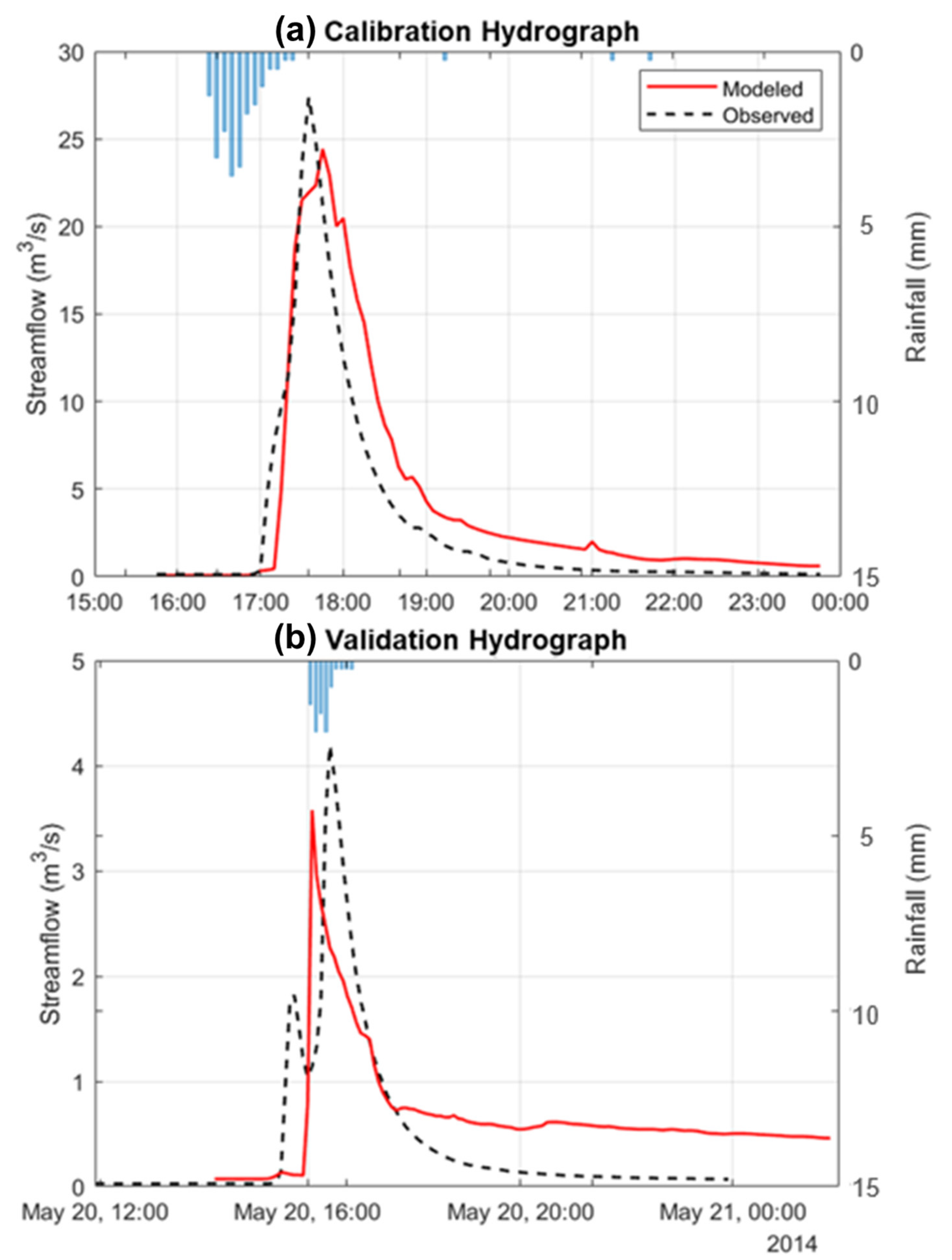
3.1. Calibration and Validation
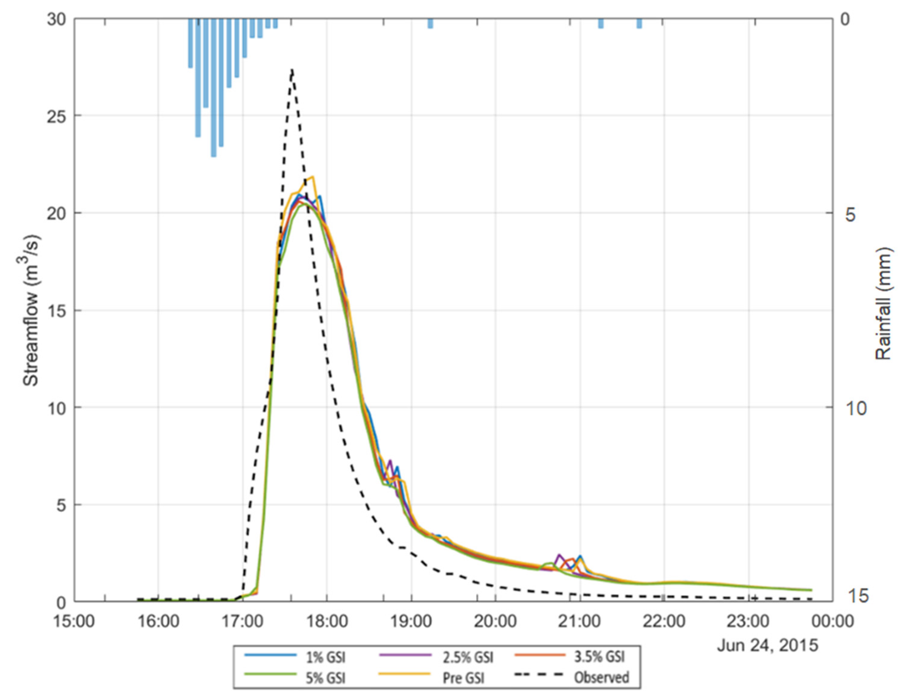
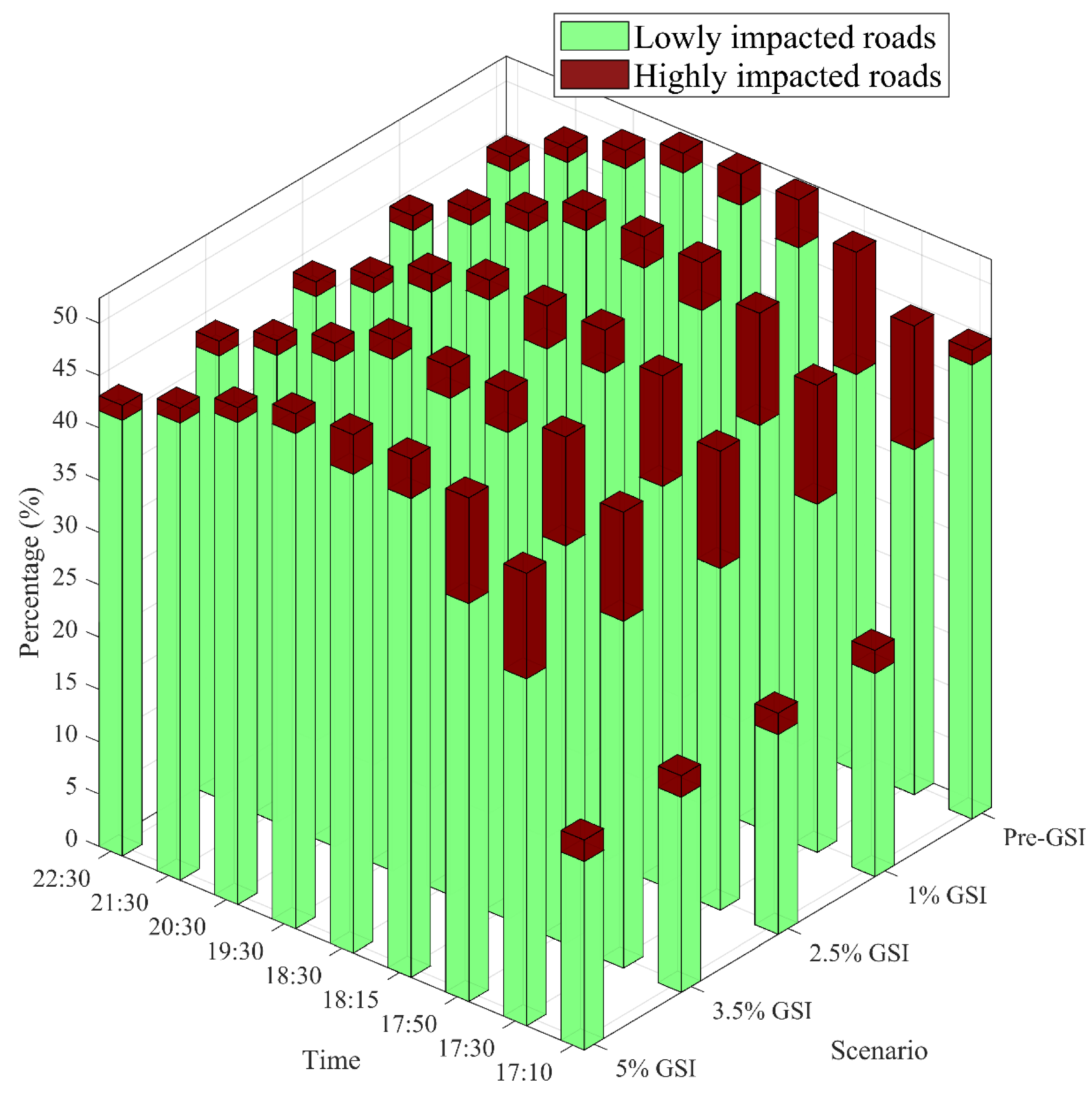
Sensitivity analysis of calibration parameters indicated that the most sensitive parameters were subcatchment slope, subcatchment width, and impervious Manning’s coefficient, while previous depression storage, hydraulic conductivity, initial deficit, and impervious depression storage were moderately sensitive parameters. The results of this sensitivity analysis were in agreement with previous studies using SWMM models [45,46]. The statistics computed comparing streamflow at the study area outfall (USGS gage 06711575) post-calibration indicates good model performance as described in [38] for all performance statistics with the exception of percent bias. The absolute value of percent bias greater than 25% indicated that the model was overpredicting streamflow for the overall storm event, although the peak streamflow was underpredicted by 5.55 m3/s (Figure 2). The validation simulation resulted in a significant reduction in model performance for prediction of streamflow at the study area outfall, suggesting that the calibrated model may not perform well for simulations of storms smaller than the calibration storm event (Table 4, Figure 2). The total volume of streamflow over the storm event was overpredicted by 36.4% for the calibration simulation and 50.2% for the validation simulation. Comparisons were made to streamflow as that is the only available quantitative data for comparison, although the model purpose was not to perfectly reproduce streamflow at the outfall but rather to represent roadway flooding within the model.
When the overall flood results (not isolating roadways) are compared with the recurring flood locations and resident reports, the reports were generally co-located with areas where flooding is modeled (Figure 3). Areas where there was either a higher frequency of larger flood depths without co-location of resident reports or vice versa were areas of concern for the general accuracy of the flood model. For example, located near where Harvard Gulch discharges into an underground rectangular conduit just upstream of the study area outfall, there was an area with depths approaching or exceeding 1 m with no occurrence of co-located citizen reports. However, as reported in the Matrix report, depths of 2.5 to 3 feet (76 to 91 cm) were observed by citizens, which indicates that modeled depths within the upper range are not necessarily due to inaccuracies [27]. The larger depths near the outfall may also be partially due to ponding of runoff at the boundary of the major system domain, as there was no 2D flow exchange across the study area boundary.

3.2. GSI Scenarios

The peak streamflow and total streamflow volume at the study area outfall were reduced for all GSI scenarios when compared to the pre-GSI scenario (Table 5). Reduction in the peak streamflow and total streamflow volume is limited at the study area outfall because the GSI scenarios drain only between 2% to 12% of the total watershed area (Table 3), which resulted in relatively smaller percent reductions in streamflow in previous studies [17]. The time of peak streamflow was not the same for all scenarios; the time of peak for the 3.5% and 5% GSI scenarios was five minutes after the 1% and 2.5% GSI scenarios, but all GSI scenarios peaked 5–10 min prior to the pre-GSI scenario. It is unexpected that the time of peak for the GSI scenarios would be less than the pre-GSI scenario, but this may be due to numerical errors in the streamflow output near the peak, as was suggested by the non-uniform shape of the output hydrograph peaks (Table 5, Figure 4).
For all GSI scenarios, the spatial extent of roadway flooding was reduced for the entirety of the storm event when compared to the baseline (pre-GSI) scenario (Figure 5). The roadway flood extent included the areas of 2D cells that overlay the roadway boundaries with water depths above the impervious depression storage depth of 0.208 cm; the flood depth was constant for the entire area of a 2D cell, and the average 2D cell area representing the roadway was approximately 0.82 km2. The roadway flood extent for all scenarios peaked at around 18:30 (Figure 5 and Figure 6), 35 min following the end of the precipitation event (16:55–18:55).
While the roadway flood extent changed similarly over time for the pre-GSI and GSI scenarios, there are slight differences in the rate at which the roadway flood extents increased to and receded from the peak extent (Figure 5). The roadway flood extent in the pre-GSI scenario increased and decreased faster than any of the GSI scenarios, at an average increased rate of 0.351 km2/hr and decreased rate of 0.0212 km2/hr. The slowest rates of increase and decrease in the GSI scenarios occurred for the 5% GSI scenario at 0.341 km2/hr and 0.0203 km2/hr, respectively. Despite having a faster rate of recession than the GSI scenarios, the pre-GSI scenario roadway flood extent was still larger than all GSI scenarios at the end of the simulation, indicating that the faster rate of recession did not overcome the increase in roadway flood extent reduction prior to the peak for the GSI scenarios. For each time shown in Figure 5, the 5% GSI scenario had the highest percent reduction in roadway flood extent, and the 1% GSI scenario had the lowest percent reduction compared to the other GSI scenarios, and for all scenarios, the largest percent reduction occurred early in the storm, prior to the peak roadway flood extent at 18:30.
The mean flood depth for all scenarios peaked at 17:30 during the peak of the precipitation event, an hour earlier than the peak roadway flood extent (Figure 5 and Figure 6). After 17:30, the mean flood depth for all scenarios decreased for the rest of the simulation, and the rate of the decrease slowed to nearly 0 cm/min as the average roadway flood depth approached 0 cm (Figure 6). Between 18:30 and 20:30, the difference in percent reduction in mean roadway depth between the smaller GSI scenarios (1% and 2.5%) and the larger scenarios (3.5% and 5%) increased notably. However, the difference in percent reduction decreased to almost zero for all scenarios by the end of the simulation, indicating that below a threshold roadway flood depth around 1 cm, an increase in the percent of DCIA converted to GSI was ineffective.
In addition to focusing on temporal variations within the storm, we also summed the difference of roadway flood extent between each GSI scenario and the pre-GSI scenario for each time shown in Figure 5 to give the total roadway flood extent reduction (km2). The total roadway flood extent reduction was largest for the 5% GSI scenario (0.35 km2 reduced) and smallest for the 1% GSI Scenario (0.066 km2 reduced). However, when the total roadway flood extent reduction was normalized by percent of DCIA converted to GSI in each scenario (i.e., the efficiency of roadway flood extent reduction), the most efficient scenario was the 2.5% GSI scenario with a total roadway flood extent reduction efficiency of 0.071 km2 reduction per percentage of DCIA converted to GSI (Figure 7a). The least efficient scenario was the 1% GSI scenario with a total roadway flood extent reduction efficiency of 0.066 km2 reduction per percentage of DCIA converted to GSI. Efficiency decreases slightly for the 3.5% and 5% GSI scenarios (Figure 7a) compared to the peak efficiency for the 2.5% GSI scenario.
This result is not replicated in the efficiency of reducing the mean roadway flood depth over the entire simulation (Figure 7b). To examine the efficiency of reducing the mean roadway flood depth, we summed the difference of mean roadway flood depth between each GSI scenario and the pre-GSI scenario for each time shown in Figure 5 to give the total mean roadway flood depth reduction (cm). The highest efficiency in reducing the mean roadway flood depth of 0.053 cm reduced per percentage of DCIA converted to GSI occurred for the 1% scenario, and the efficiency decreased as the percentage of DCIA converted increased, with the lowest efficiency of 0.028 cm per percentage of DCIA converted to GSI for the 5% GSI scenario.
The area shown in Figure 8 was of interest because of the multiple resident reports of flooding in the area and a location of recurring flooding identified by the City and County of Denver. These reports were co-located with larger flood depths that persist through 19:30 in both scenarios, indicating that the surface flood model was generally and qualitatively representing flooding patterns that would be expected for this area within the watershed. There was a clear difference in the flood extent and distribution of depths between the Pre and 5% GSI scenarios that occur at 17:30, and the difference was especially pronounced in the NW portion of the inset. Additionally, the results shown in this area support the assumption made that the influence of existing surface storages within the watershed could be approximated using the elevation difference within the 2D surface model. The cells with the largest depths were co-located with the surface detention polygon located within this area of interest (Figure 8).

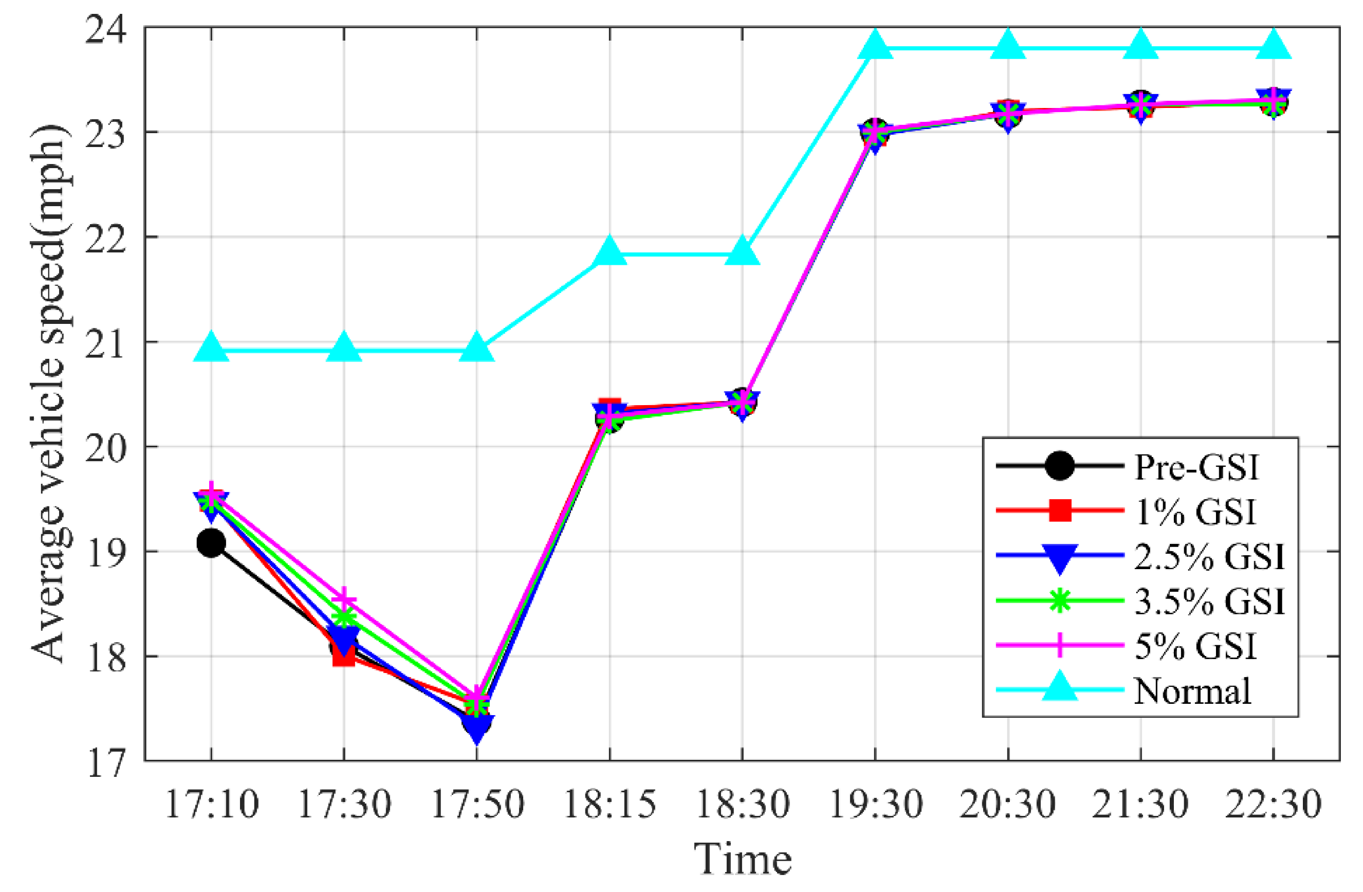
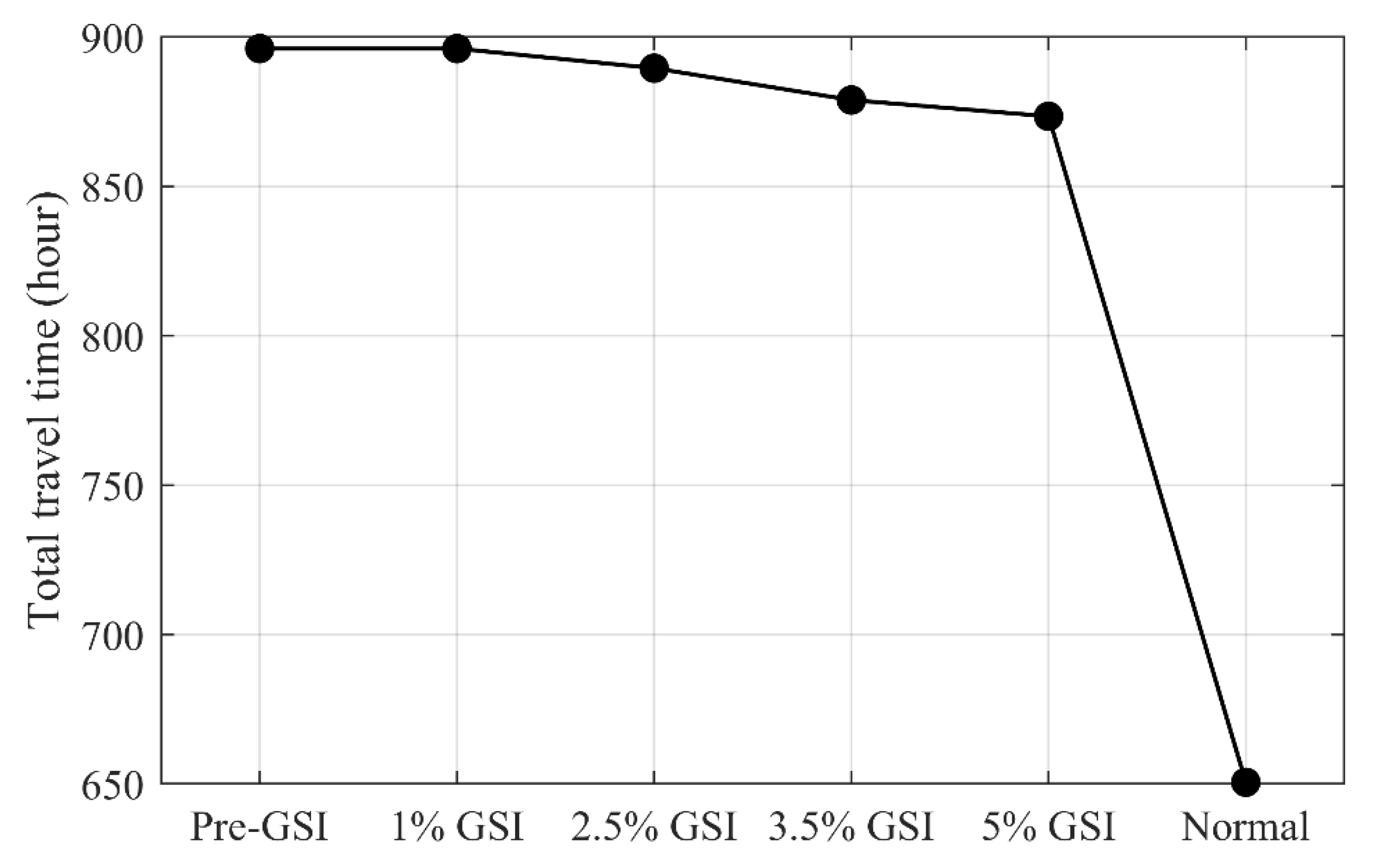
3.3. Traffic Analysis

To examine the effects of flooding on the transportation network, we simulated vehicle speed reduction in roadways in the study area. Flooded roads were classified into two types: lowly impacted roads with a maximum vehicle speed reduction of less than or equal to 25%, and highly impacted roads with a maximum vehicle speed reduction of more than 25%. Lowly impacted roads account for the majority of flooded roads in each scenario (Figure 9). Over the storm, the numbers of both lowly and highly impacted roads first increased and then decreased. The percentage of highly impacted roads reached its maximum value at 17:30, whereas that of lowly impacted roads reached its maximum value at 19:30. In the pre-GSI scenario, the maximum percentage of lowly and highly impacted roads were 50% and 12%, respectively. More GSI reduced the flood impact on both high and low impacted roads.
We also examined the average speed of all vehicles in the transportation network in five flooding scenarios (pre-GSI, 1%, 2.5%, 3.5%, and 5% GSI) and one normal (dry) weather scenario with SUMO (Figure 10). Flooding could greatly reduce traffic speed, especially seen in differences between 17:10 and 17:50 in flooded scenarios and the normal scenario. For example, compared to the normal scenario, the average vehicle speed of the pre-GSI scenario decreased by 9%, 14%, and 17% at 17:10, 17:30, and 17:50, respectively. For each of those five scenarios, the average vehicle speed started to decrease at 17:10 and reached the minimum value at 17:50. During this period, the traffic demand remains the same, so the roadway flooding was the cause of differences. The mean roadway flood depth increased with time from 17:10 and reached the maximum value at 17:30 (Figure 6). The peak value of average vehicle speed occurred 20 min later (17:50) than the minimum value of the mean roadway depth (17:30), which may be because the increase in the number of flooded roads plays a more dominant role than the mean roadway flood depth.
In the later part of the simulation (from 17:50 to 22:30), the average vehicle speed increases with time (Figure 10). There are two jumps occurring from 17:50 to 18:15 and from 18:30 to 19:30. This is because of the reduction in traffic demand, which is also reflected in traffic speed variation under normal conditions. During the period 18:15 to 18:30 and 19:30 to 22:30, the roadway flood depth decreased relatively slowly, which led to a gradual increase in the average vehicle speed. GSI can increase the average vehicle speed, especially between 17:10 and 17:50 when the vehicle speed was the lowest. In general, a higher GSI percentage leads to a larger improvement in traffic performance. For example, 5% GSI could increase the average vehicle speed by 2.5% at 17:30.
We also examined the total travel time of all vehicle trips during the simulation period under different scenarios (Figure 11). The total travel time decreased as the GSI percentage increases. For example, compared to the pre-GSI scenario, 5% GSI reduced the total travel time by around 23 h (i.e., 2.5%). This indicates that GSI could effectively improve the traffic performance of flooded transportation networks.

4. Discussion

The results described above indicated that the conversion of even 1% of the DCIA to GSI lead to the reduction in mean roadway flood depth and spatial extent, and increasing the amount of GSI added to 5% of the DCIA further reduced the mean roadway flood depth and spatial extent (Figure 5 and Figure 6). Previous studies examining impacts of GSI on urban flood depths at stormwater nodes found that the minimum percentage of DCIA converted to GSI necessary to observe an impact was between 5% and 20% converted [4,47,48]. The reduction seen in this study at 1% DCIA converted to GSI suggests that, although the other studies examined different watersheds, GSI types, storms, and modeling procedures, modeling urban flooding as a 2D surface may be more sensitive to the addition of GSI than when floods are only examined at stormwater nodes.
The difference in percent reduction in both roadway flood extent and mean depth with GSI was most pronounced in the first 20–40 min of the simulation results, smallest around the peak, and then increased slowly for the remainder of the simulation (Figure 5 and Figure 6). Increasing the percentage of DCIA converted to GSI had the largest effect during the precipitation event, but the effects were less pronounced as the flood extent and mean depth approached their peak values (Figure 5b and Figure 6b). The flood metrics of depth and extent differ in their response to the addition of GSI, although in both cases, additional GSI conversion beyond 2.5% of DCIA yielded diminishing returns (Figure 7).
All results of this study must be considered within the context of the limitations of the modeling methods used. In the models developed for this study, the GSI was not spatially represented. Instead, the effects of the GSI, specifically bioretention cells, were distributed evenly throughout the impervious area of the subcatchment. Therefore, the percent reduction in spatial extent and flood depth on the roadway cannot be attributed to the specific placement of GSI. Additional reduction in roadway flooding that may occur due to run-on from areas surrounding the GSI was not accounted for with this method of GSI representation.
Although there are methods available in PCSWMM that allow for the spatial application of GSI by creating individual subcatchments for each GSI unit, this methodology is not conducive to the addition of large numbers of GSI to the model. In this study, between 566 and 3158 GSI units were added to the 1% and 5% GSI scenarios, respectively, and to represent these spatially as individual subcatchments would require placement and parameter assignment manually. In addition to the high labor demand of implementing spatial GSI, the addition of over 500 GSI represented as small 22.3 × 10⁻⁵ km2 subcatchments, would lead to an even greater computational demand that may be time prohibitive. The impact of not modeling the specific locations of GSI on the accuracy of results of 2D surface floods has not been assessed by the current body of research but has been noted as a limitation in previous studies [22].
For a more detailed understanding of how GSI placement affects roadway flooding, the ability to automate placement and parameter assignment for representative GSI subcatchments within PCSWMM as an input data file would greatly improve the efficiency of modeling spatially representative GSI units. Additionally, there is a discrepancy in the studies that have examined theoretical GSI network effects on urban flooding [9,15,19] and the study of how realistic GSI network scenarios based on municipality future plans affect urban flooding. However, before embarking on the further development of complex dual-drainage models, the fundamental challenge of complete and accurate input data, including stormwater network data, soil data, and precipitation data, is necessary.
A primary challenge influencing the reliability and uncertainty of the simulation results is the short (single event) calibration simulation and the lack of data available to calibrate the 2D surface flooding component of the model. The only available data for calibration within the study area is streamflow at the USGS outlet gage, therefore to develop a model that could be calibrated using USGS streamflow data at the watershed outlet, the study area had to include all area that would drain via surface runoff and the stormwater network to the stream channel at the USGS gage. Often, stormwater models are calibrated using long-term simulations with multiple storm events of varying characteristics, including the interaction between antecedent conditions of successive storm events with runoff. However, because of the long simulation times and computational demand of the model used in this study, calibration simulation run times for a limited number of parameters (Table 1) for a single storm event exceeded 60 h. In order to calibrate for a continuous precipitation record containing multiple storms, a larger computational capacity would be required. The model calibration for streamflow resulted in calibration statistics that are characteristic of a “good” model [38] (Table 4). When the model was tested for a validation storm that has a total rainfall that is 12.1 mm smaller than the storm used as the calibration event, the quality of the modeled streamflow compared to observed data deteriorated considerably (Table 4). This indicates that although the model was adequately calibrated for the single storm event used to simulate all scenarios, the transferability of the model to other storm events was poor. In order to improve the accuracy of this type of model for the full range of storm event sizes, a larger computational capacity would be needed to calibrate the model for a continuous, longer-term precipitation record.
In addition to challenges calibrating the dual-drainage model with available streamflow data, the complete absence of quantitative roadway flood depth data does not allow for a test of the reliability of modeled roadway flooding depth results. The method used to model flooding in this study results in detailed local flood extent and depth results (Figure 8), but without accurate observations of flooding, localized variations cannot be verified. A potential solution to the lack of urban flood observation data is the utilization of resident (311) reports of flooding and known recurring flood locations defined by the City and County of Denver. These reports rarely contain quantitative information on the depth or distribution of flooding, and therefore, their utility for validation is limited to co-location with modeled flooding (Figure 3 and Figure 8). Additionally, the number, distribution, and range of flood depths of reports pertaining to a single storm event were not large enough to validate flood data within an entire watershed. Crowdsourced science and/or resident reports to municipalities have the potential to increase the number of observations of urban flooding [23].

5. Conclusions

Modeling stormwater structure-scale interaction between green stormwater infrastructure (GSI), surface runoff, and stormwater networks to examine the extent, depth, and distribution of 2D roadway flooding within a watershed is critical for expanding the understanding of how GSI impact urban systems such as transportation networks. With a detailed dual-drainage model of Harvard Gulch, Denver, Colorado, and five GSI scenarios applied as a percentage of the directly-connected impervious area (DCIA) converted to bioretention cells; it was shown that even at 1% of the DCIA converted to GSI, there was a decrease in the extent and mean depth of roadway flooding, as well as localized changes to flood extent and distribution of depths. Using the SUMO traffic model, we saw that this reduction in roadway flooding with GSI led to decreases in total vehicle travel time and increases in vehicle speed, especially during the most flooded part of the storm. This study provides an example of a watershed-scale, detailed dual-drainage model and identifies challenges that can be used to direct future work on the structure-scale interaction between GSI, stormwater structures, 2D surface runoff, and traffic.
  • How can 1D–2D dual-drainage modeling help determine the effect of GSI networks on the depth, flooded extent, and spatial distribution of roadway flooding?
    • The modeled streamflow results showed that for this specific storm event, the dual-drainage model could provide realistic streamflow outputs (Figure 2), which for a model without a 2D flood domain would indicate acceptable model performance (Table 4).
    • With an understanding of the reliability of results, the major system flood model was able to show that the conversion of only 1% DCIA to GSI reduced the spatial extent (Figure 5) and mean depth (Figure 6) of roadway flooding, particularly during the beginning and end of the storm response.
    • Conversion of increasing percentages of DCIA to GSI (1%, 2.5%, 3.5%, and 5%) further reduced the flood spatial extent and flood mean depth (Figure 5 and Figure 6), although with diminishing returns (Figure 7).
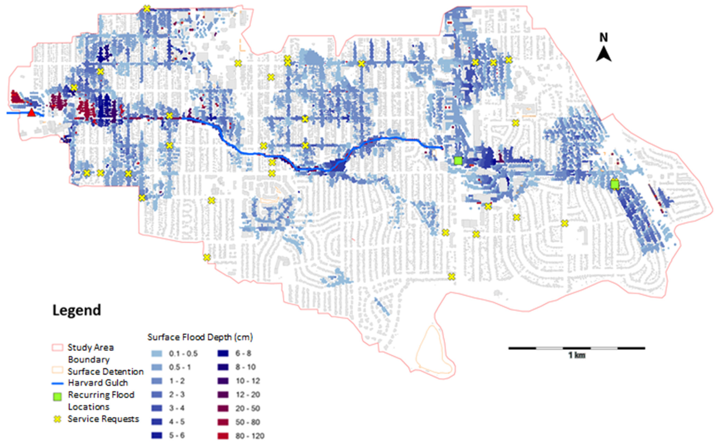
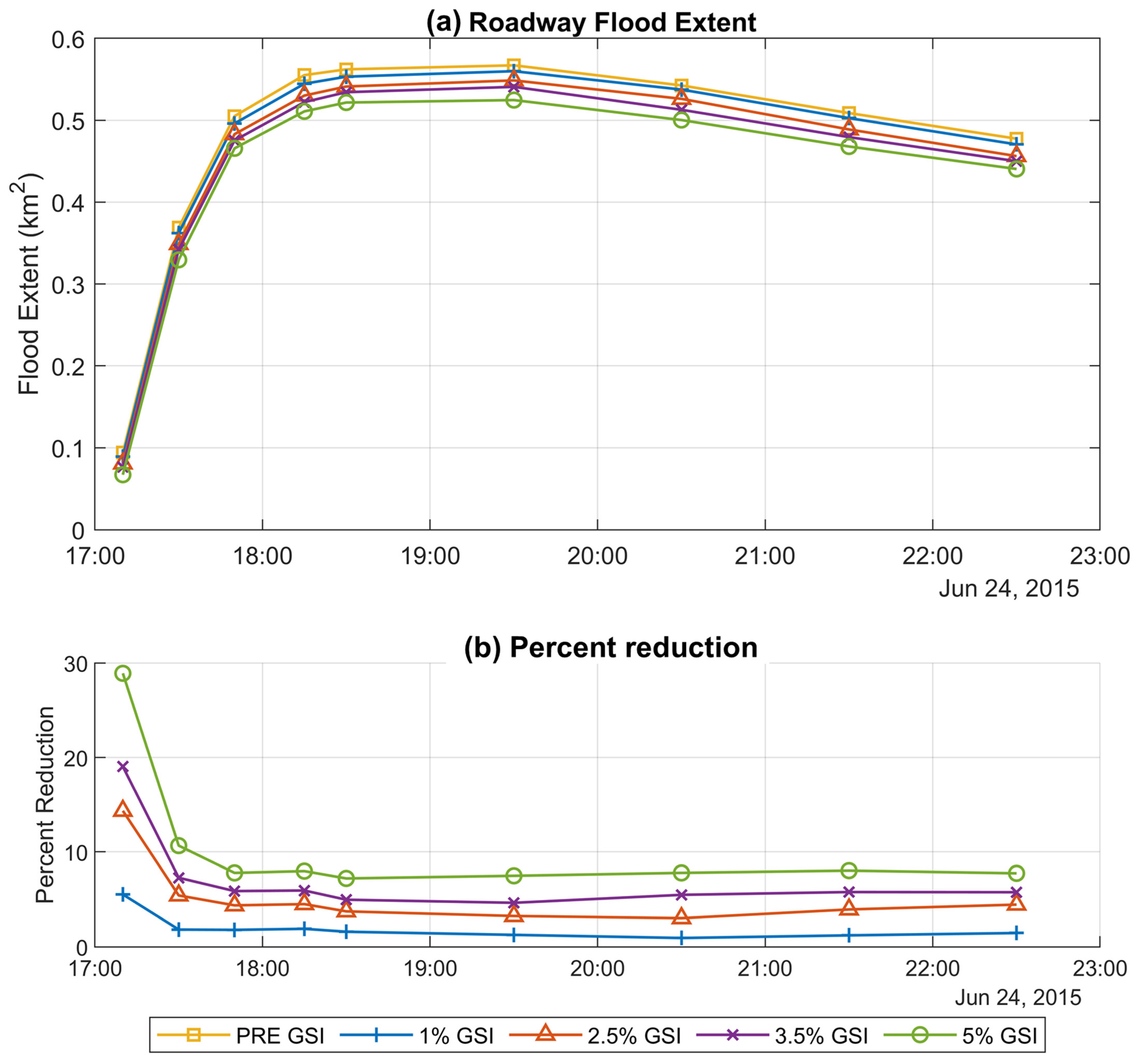
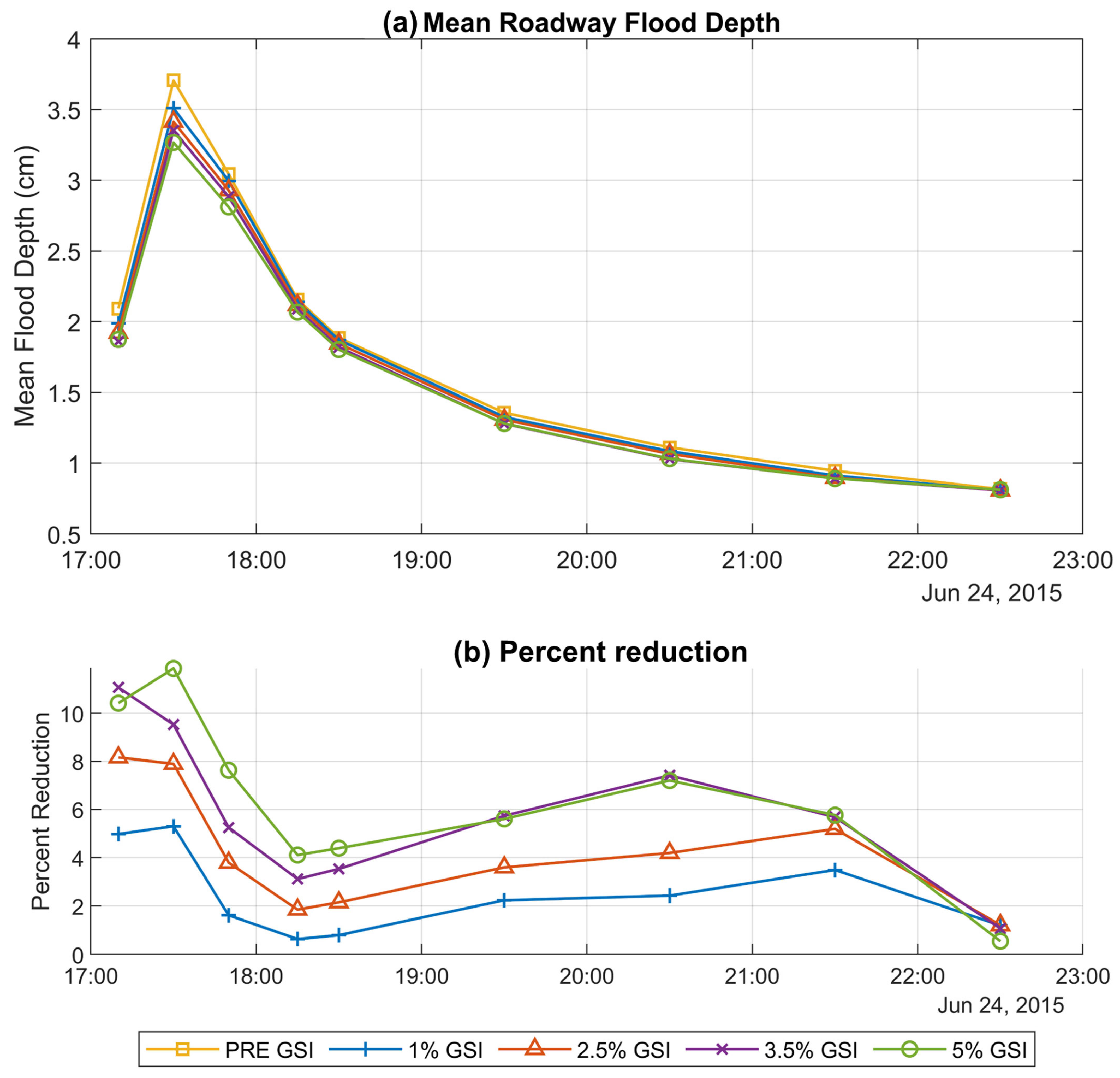
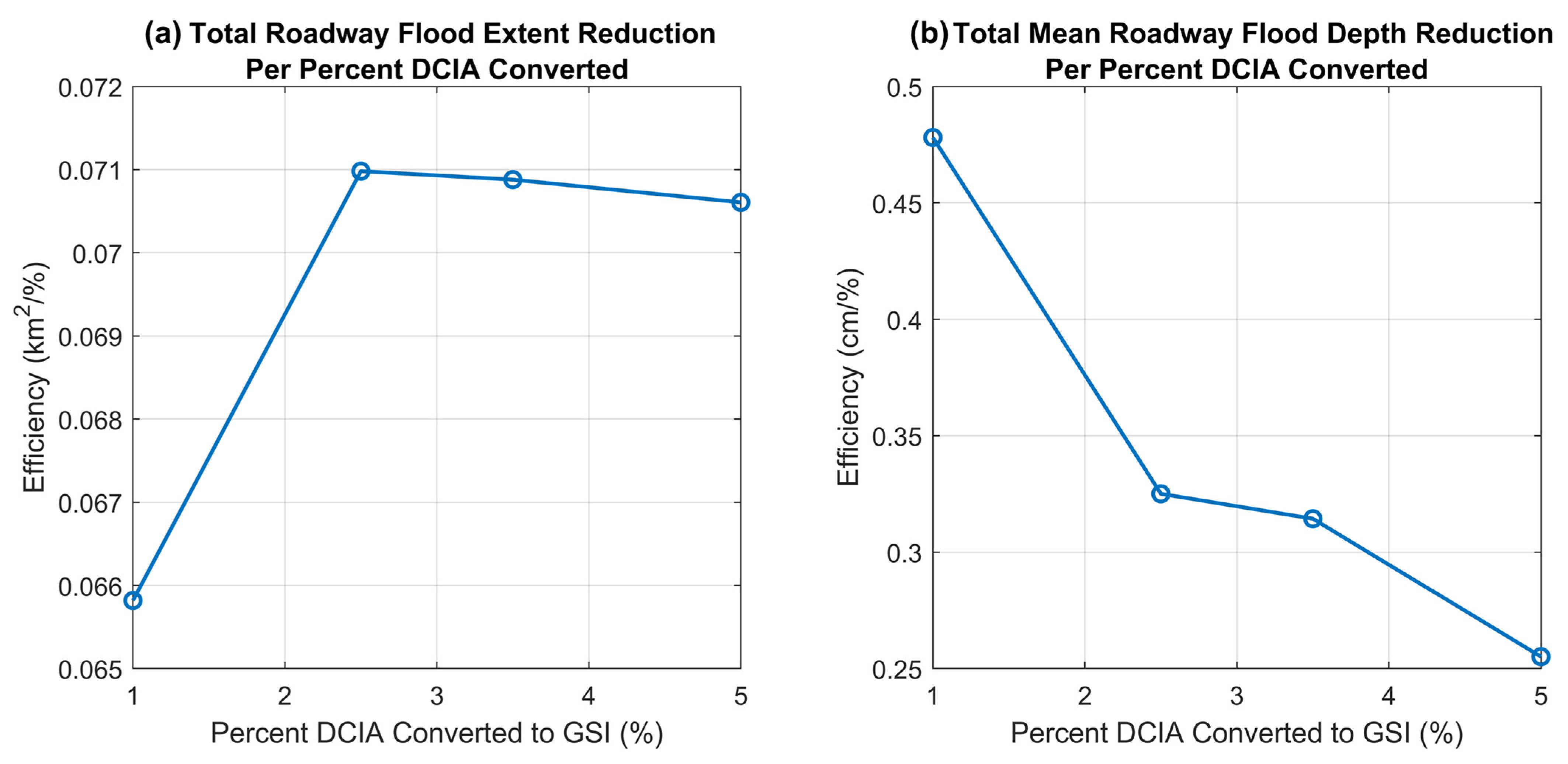
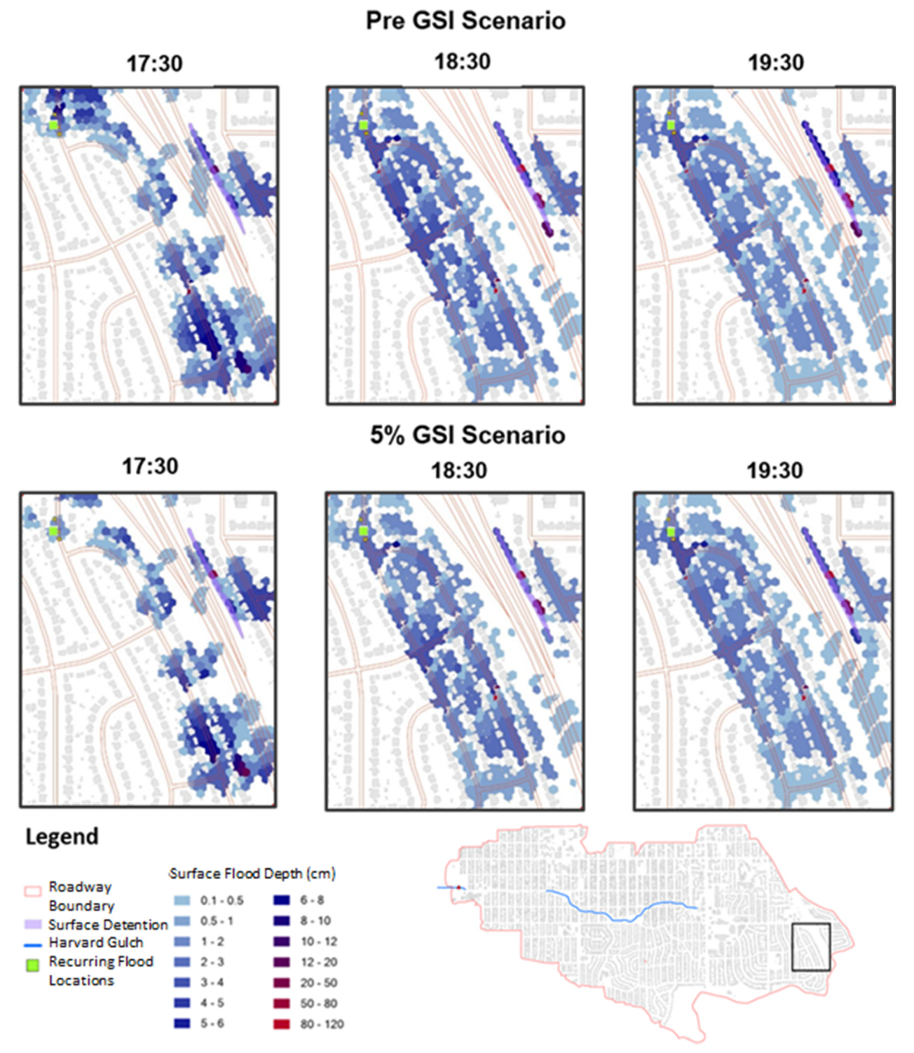
    • Results of the major system flood model showed localized variation in flooding that indicates the value of a dual-drainage model in understanding the structure-scale interactions between GSI, stormwater structures, and runoff, given that these results could be verified by observation of urban flooding (Figure 3 and Figure 8).
  • How do GSI networks affect the performance of the traffic system during a storm event?
    • Reduced roadway flooding led to increased average vehicle speeds (Figure 10) and a decrease in the percentage of roads impacted by flooding (Figure 9) and total travel time (i.e., 23 h of 2.5% for the 5% GSI scenario) (Figure 11).
  • What are the limitations of dual-drainage 1D–2D modeling for characterizing the effects of GSI networks on roadway flooding?
    • The model developed lacks spatially-specific GSI network implementation as the model methods to represent GSIs in space were not scalable to large watersheds. Future work to improve the incorporation of spatially-specific GSIs efficiently into stormwater models will clarify the importance of this challenge.
    • Although we knew that the specific storm event modeled produced roadway flooding, there was not spatially distributed data on the depth and timing of roadway flooding that could be used to compare to modeled roadway flooding model results. Crowdsourced science and resident reporting have the potential to provide critically needed calibration data for urban flooding, but a significant increase in the quantity and distribution of these reports is needed.
    • Additional computational capacity is needed to calibrate a 1D–2D dual-drainage model of this size and complexity using a continuous long-term precipitation and streamflow record.
There is the potential that, with the continued improvement of modeling techniques and technology as well as efforts to improve input and calibration data, the development of detailed watershed-scale dual-drainage models can address gaps in the understanding of structure-scale interactions over the entirety of a study watershed.

Author Contributions

Conceptualization, K.L.K., A.S.B., and S.C.; Investigation, K.L.K. and G.H.; writing—original draft preparation, K.L.K. and G.H.; writing—review and editing, K.L.K., G.H., A.S.B., and S.C.; visualization, K.L.K. and G.H.; supervision, A.S.B. and S.C.; project administration, A.S.B.; funding acquisition, A.S.B. and S.C. All authors have read and agreed to the published version of the manuscript.

Funding

This work was partly supported by the Mountain-Plains Consortium, a University Transportation Center funded by the U.S. Department of Transportation, the Colorado Water Center, and NSF award 1805340.

Institutional Review Board Statement

Not applicable.

Informed Consent Statement

Not applicable.

Data Availability Statement

The data presented in this study are openly available in CUAHSI HydroShare at https://doi.org/10.4211/hs.6d6216f4973c45b6be80b3ce5e3e6764 or were obtained from the Denver Regional County of Governments and the City and County of Denver and are available from these third parties.

Acknowledgments

We acknowledge S. Kampf and M. Arabi for their valuable input and perspective and C. Williams for assistance in compiling observational datasets. We also acknowledge Computation Hydraulics International for their support through technology grants and access to PCSWMM software and the Matrix Design group for providing valuable background information and stormwater modeling that supported this project.

Conflicts of Interest

The authors declare no conflict of interest.

Appendix A

Data Gap Filling Approach

Even after consulting available as-built drawings, there was a large proportion of stormwater structures with incomplete or missing structure details that required the development of a process to fill or correct structure details using the most relevant known information about the individual and surrounding structures. Of the stormwater data available from the City and County of Denver for the study area, 78% of inlets, 28% of manholes, 6.6% of conduits, and 85% of the surface and underground storage facilities were missing one or more important structure details. The goal of this process was to maximize the accuracy of structure-specific input data for the stormwater network. Along with the process for filling and correcting structure details, assumptions made in determining input values are described below:
1.
If a junction is missing attribute data, the value may be recorded in one of the connected conduits;
2.
If a junction is missing invert details:
a
If connected conduits have invert data, use the lowest connected conduit invert;
b
If connected conduits do not have invert data:
i
Use length and slope attributes from connected conduits and known junction invert to compute;
ii
If connected conduits have missing slope attribute:
  • For inlets:
    (1)
    If inlet type is known, use default inlet depth based on inlet type from the city and county of Denver standard specifications;
    (2)
    If the inlet type is unknown, use the default connected conduit slope of 2% (based on Denver standard specification).
  • For manholes, assume the nearest known slope is continuous and extrapolate from the nearest known junction attribute:
    (1)
    Some junctions in the stormwater network data represent a pipe-to-pipe connection. The invert of these is interpolated from the nearest known junction invert using the conduit slope.
3.
If the ground elevation of an inlet or manhole is unknown, use the 1 m DEM elevation;
4.
Conduit offsets were computed from the difference between known conduit inverts and junction inverts:
  • If only the upstream or downstream conduit invert was known, the missing invert was computed using the slope and length, and then the offset was computed;
  • If neither upstream or downstream conduit inverts, or the slope were known, the offset was assumed to be zero;
  • If a zero offset resulted in a negative conduit slope, the slope was assumed to be the same as a neighboring in-line conduit, and the offset was recomputed.
5.
If conduit geometry is unknown, it was assumed to be the same as the nearest known conduit geometry.
To complete the minor system, the stormwater network was audited using tools available in PCSWMM. Orphans, stormwater structures that are not connected to any other structure, were removed. In some cases, the approximations of invert or offset values described above resulted in a negative or zero slope, indicating an overestimation of the unknown value. There are tools available in PCSWMM to automatically modify conduit slopes, but the over-utilization of these tools would have overridden much of the known invert and slope values, negating the value of the tool’s efficiency. Instead, the invert approximations that caused negative or zeros slopes were manually adjusted to preserve neighboring data. The decision-making framework could not be applied to areas in the stormwater network with clusters of structures with unknown details. These clusters were removed, and it was assumed that the runoff generated from the surrounding area would enter the minor system at the nearest known downstream inlet. Though simplifying the network may have led to localized errors in the overland flow, the overall inputs to the minor system were not expected to be significantly altered. The contributing areas to the simplified network are relatively small and typically isolated on private property, such as the Denver University campus, where roadway flooding was not a concern for this study.

References

  1. Shuster, W.D.; Bonta, J.; Thurston, H.; Warnemuende, E.; Smith, D.R. Impacts of Impervious Surface on Watershed Hydrology: A Review. Urban Water J. 2005, 2, 263–275. [Google Scholar] [CrossRef]
  2. Lee, J.G.; Selvakumar, A.; Alvi, K.; Riverson, J.; Zhen, J.X.; Shoemaker, L.; Lai, F. A Watershed-Scale Design Optimization Model for Stormwater Best Management Practices. Environ. Model. Softw. 2012, 37, 6–18. [Google Scholar] [CrossRef]
  3. Perez-Pedini, C.; Limbrunner, J.; Vogel, R. Optimal Location of Infiltration-Based Best Management Practices for Storm Water Management. J. Water Resour. Plan. Manag. 2005, 131, 441–448. [Google Scholar] [CrossRef]
  4. Zellner, M.; Massey, D.; Minor, E.; Gonzalez-Meler, M. Exploring the Effects of Green Infrastructure Placement on Neighborhood-Level Flooding via Spatially Explicit Simulations. Comput. Environ. Urban Syst. 2016, 59, 116–128. [Google Scholar] [CrossRef] [Green Version]
  5. Field, C.B.; Barros, T.F.V.; Stocker, D.; Qin, D.J.; Dokken, K.L.; Ebi, M.D.; Mastrandrea, K.J.; Mach, G.-K.; Plattner, S.K.; Allen, M.; et al. (Eds.) Managing the Risks of Extreme Events and Disasters to Advance Climate Change Adaptation: Special Report of the Intergovernmental Panel on Climate Change; Cambridge University Press: Cambridge, UK, 2012; ISBN 978-1-139-17724-5. [Google Scholar]
  6. Galloway, G.E.; Reilly, A.; Ryoo, S.; Riley, A.; Haslam, M.; Brody, S.; Highfield, W.; Gunn, J.; Rainey, J.; Parker, S. The Growing Threat of Urban Flooding: A National Challenge; University of Maryland: College Park, MD, USA; Texas A&M University: College Station, TX, USA, 2018. [Google Scholar]
  7. Schmitt, T.; Thomas, M.; Ettrich, N. Analysis and Modeling of Flooding in Urban Drainage Systems. J. Hydrol. 2004, 299, 300–311. [Google Scholar] [CrossRef]
  8. Jacobs, J.M.; Cattaneo, L.R.; Sweet, W.; Mansfield, T. Recent and Future Outlooks for Nuisance Flooding Impacts on Roadways on the U.S. East Coast. Transp. Res. Rec. J. Transp. Res. Board 2018, 2672, 1–10. [Google Scholar] [CrossRef]
  9. Pregnolato, M.; Ford, A.; Dawson, R. Disruption and Adaptation of Urban Transport Networks from Flooding. E3s Web Conf. 2016, 7, 07006. [Google Scholar] [CrossRef] [Green Version]
  10. Pyatkova, K.; Chen, A.S.; Butler, D.; Vojinović, Z.; Djordjević, S. Assessing the Knock-on Effects of Flooding on Road Transportation. J. Environ. Manag. 2019, 244, 48–60. [Google Scholar] [CrossRef] [PubMed]
  11. Pregnolato, M.; Ford, A.; Glenis, V.; Wilkinson, S.; Dawson, R. Impact of Climate Change on Disruption to Urban Transport Networks from Pluvial Flooding. J. Infrastruct. Syst. 2017, 23, 04017015. [Google Scholar] [CrossRef] [Green Version]
  12. Yin, J.; Yu, D.; Yin, Z.; Liu, M.; He, Q. Evaluating the Impact and Risk of Pluvial Flash Flood on Intra-Urban Road Network: A Case Study in the City Center of Shanghai, China. J. Hydrol. 2016, 537, 138–145. [Google Scholar] [CrossRef] [Green Version]
  13. Hou, G.; Chen, S.; Zhou, Y.; Wu, J. Framework of Microscopic Traffic Flow Simulation on Highway Infrastructure System under Hazardous Driving Conditions. Sustain. Resilient Infrastruct. 2017, 2, 136–152. [Google Scholar] [CrossRef]
  14. Askarizadeh, A.; Rippy, M.A.; Fletcher, T.D.; Feldman, D.; Peng, J.; Bowler, P.; Mehring, A.; Winfrey, B.; Vrugt, J.; AghaKouchak, A.; et al. From Rain Tanks to Catchments: Use of Low-Impact Development to Address Hydrologic Symptoms of the Urban Stream Syndrome. Environ. Sci. Technol. 2015. [Google Scholar] [CrossRef] [PubMed] [Green Version]
  15. Qin, H.; Li, Z.; Fu, G. The Effects of Low Impact Development on Urban Flooding under Different Rainfall Characteristics. J. Environ. Manag. 2013, 129, 577–585. [Google Scholar] [CrossRef] [PubMed] [Green Version]
  16. Jefferson, A.J.; Bhaskar, A.S.; Hopkins, K.G.; Fanelli, R.; Avellaneda, P.M.; McMillan, S.K. Stormwater Management Network Effectiveness and Implications for Urban Watershed Function: A Critical Review. Hydrol. Process. 2017, 31, 4056–4080. [Google Scholar] [CrossRef]
  17. Bell, C.D.; Wolfand, J.M.; Panos, C.L.; Bhaskar, A.S.; Gilliom, R.L.; Hogue, T.S.; Hopkins, K.G.; Jefferson, A.J. Stormwater Control Impacts on Runoff Volume and Peak Flow: A Meta-Analysis of Watershed Modeling Studies. Hydrol. Process. 2020, 34, 3134–3152. [Google Scholar] [CrossRef]
  18. Rossman, L.; Huber, W. Storm Water Management Model Reference Manual: Volume I—Hydrology (Revised); US Environmental Protection Agency: Cincinnati, OH, USA, 2016. [Google Scholar]
  19. Zhu, Z.; Chen, X. Evaluating the Effects of Low Impact Development Practices on Urban Flooding under Different Rainfall Intensities. Water 2017, 9, 548. [Google Scholar] [CrossRef]
  20. Liwanag, F.; Mostrales, D.S.; Ignacio, M.T.T.; Orejudos, J.N. Flood Modeling Using GIS and PCSWMM. Eng. J. 2018, 22, 279–289. [Google Scholar] [CrossRef]
  21. Djordjević, S.; Prodanović, D.; Maksimović, Č. An Approach to Simulation of Dual Drainage. Water Sci. Technol. 1999, 39, 95–103. [Google Scholar] [CrossRef]
  22. Elliott, A.H.; Trowsdale, S.A. A Review of Models for Low Impact Urban Stormwater Drainage. Environ. Model. Softw. 2007, 22, 394–405. [Google Scholar] [CrossRef]
  23. Smith, B.K.; Rodriguez, S. Spatial Analysis of High-Resolution Radar Rainfall and Citizen-Reported Flash Flood Data in Ultra-Urban New York City. Water 2017, 9, 736. [Google Scholar] [CrossRef] [Green Version]
  24. NOAA Climate at a Glance|National Centers for Environmental Information (NCEI). Available online: https://www.ncdc.noaa.gov/cag/county/mapping/5/pcp/201911/12/value (accessed on 19 June 2020).
  25. City and County of Denver Green Infrastructure Implementation Strategy. Available online: https://www.denvergov.org/content/denvergov/en/wastewater-management/stormwater-quality/green-infrastructure/implementation.html (accessed on 19 June 2020).
  26. MacKenzie, K.; Urbonas, B.; Jansekok, M.; Guo, J.C.Y. Effect of Raingage Density on Runoff Simulation Modeling. In World Environmental and Water Resources Congress 2007: Restoring Our Natural Habitat; American Society of Civil Engineers: Reston, VA, USA, 2007; pp. 1–11. [Google Scholar] [CrossRef]
  27. Matrix Design Group. Harvard Gulch and Dry Gulch Major Drainageway Plan: Conceptual Design Report; Matrix Design Group: Denver, CO, USA, 2016. [Google Scholar]
  28. Alley, W.M.; Veenhuis, J.E. Effective Impervious Area in Urban Runoff Modeling. J. Hydraul. Eng. 1983, 109, 313–319. [Google Scholar] [CrossRef]
  29. City and County of Denver Denver Open Data Catalog. Available online: https://www.denvergov.org/opendata/ (accessed on 19 June 2020).
  30. NRCS, Natural Resources Conservation Service, United States Department of Agriculture Web Soil Survey. Available online: https://websoilsurvey.sc.egov.usda.gov/App/HomePage.htm (accessed on 18 December 2020).
  31. CHI Water Computational Hydraulics International (CHI). Available online: https://www.chiwater.com/Home (accessed on 19 June 2020).
  32. McCuen, R. Hydrologic Analysis and Design, 4th ed.; Pearson: Boston, MA, USA, 2016; ISBN 978-0-13-431312-2. [Google Scholar]
  33. Rawls, W.J.; Brakensiek, D.L.; Miller, N. Green-ampt Infiltration Parameters from Soils Data. J. Hydraul. Eng. 1983, 109, 62–70. [Google Scholar] [CrossRef] [Green Version]
  34. City and County of Denver Department of Public Works. Transportation Standards and Details for the Engineering Division; City and County of Denver Department of Public Works: Denver, CO, USA, 2017. [Google Scholar]
  35. City and County of Denver Department of Public Works. City and County of Denver Storm Drainage Design and Technical Criteria; City and County of Denver Department of Public Works: Denver, CO, USA, 2013. [Google Scholar]
  36. James, W. Rules for Responsible Modeling; CHI: Guelph, ON, Canada, 2003; ISBN 978-0-9683681-5-2. [Google Scholar]
  37. Mile High Flood District Criteria Manual Volume 3. Available online: https://mhfd.org/resources/criteria-manual-volume-3/ (accessed on 7 July 2020).
  38. Moriasi, D.N.; Arnold, J.G.; van Liew, M.W.; Bingner, R.L.; Harmel, R.D.; Veith, T.L. Model Evaluation Guidelines for Systematic Quantification of Accuracy in Watershed Simulations. Trans. Asabe 2007, 50, 885–900. [Google Scholar] [CrossRef]
  39. City and County of Denver Ultra-Urban Green Infrastructure Guidelines. Available online: https://www.denvergov.org/content/denvergov/en/wastewater-management/stormwater-quality/ultra-urban-green-infrastructure.html (accessed on 19 June 2020).
  40. Zhao, H.; Zou, C.; Zhao, J.; Li, X. Role of Low-Impact Development in Generation and Control of Urban Diffuse Pollution in a Pilot Sponge City: A Paired-Catchment Study. Water 2018, 10, 852. [Google Scholar] [CrossRef] [Green Version]
  41. Lopez, P.A.; Behrisch, M.; Bieker-Walz, L.; Erdmann, J.; Flötteröd, Y.-P.; Hilbrich, R.; Lücken, L.; Rummel, J.; Wagner, P.; WieBner, E. Microscopic Traffic Simulation Using Sumo. In Proceedings of the 2018 21st International Conference on Intelligent Transportation Systems (ITSC), Maui, HI, USA, 4–7 November 2018; pp. 2575–2582. [Google Scholar]
  42. Fereshtehpour, M.; Burian, S.J.; Karamouz, M. Flood Risk Assessments of Transportation Networks Utilizing Depth-Disruption Function. In World Environmental and Water Resources Congress 2018: Water, Wastewater, and Stormwater; Urban Watershed Management; Municipal Water Infrastructure; and Desalination and Water Reuse; American Society of Civil Engineers: Reston, VA, USA, 2018; pp. 134–142. [Google Scholar] [CrossRef]
  43. Yang, Y.; Ng, S.T.; Zhou, S.; Xu, F.J.; Li, H. A Physics-Based Framework for Analyzing the Resilience of Interdependent Civil Infrastructure Systems: A Climatic Extreme Event Case in Hong Kong. Sustain. Cities Soc. 2019, 47, 101485. [Google Scholar] [CrossRef]
  44. OpenStreetMap. Available online: https://www.openstreetmap.org/ (accessed on 20 December 2020).
  45. Panos, P.C.; Hogue, T.S.; Gilliom, R.; McCray, J. High-Resolution Modeling of Infill Development Impact on Stormwater Dynamics in Denver, Colorado. J. Sustain. Water Built Environ. 2018, 4, 04018009. [Google Scholar] [CrossRef]
  46. Rosa, D.J.; Clausen, J.C.; Dietz, M.E. Calibration and Verification of SWMM for Low Impact Development. J. Am. Water Resour. Assoc 2015, 51, 746–757. [Google Scholar] [CrossRef]
  47. Palla, A.; Gnecco, I. Hydrologic Modeling of Low Impact Development Systems at the Urban Catchment Scale. J. Hydrol. 2015, 528, 361–368. [Google Scholar] [CrossRef]
  48. Walsh, T.C.; Pomeroy, C.A.; Burian, S.J. Hydrologic Modeling Analysis of a Passive, Residential Rainwater Harvesting Program in an Urbanized, Semi-Arid Watershed. J. Hydrol. 2014, 508, 240–253. [Google Scholar] [CrossRef]
Figure 1. Study area including the location of the study area outfall USGS stream gage 06711575 (left), USGS stream gage 06711570, and rain gages. The fifth rain gage is co-located at USGS stream gage 06711575.
Water 13 01563 g001
Figure 2. (a) Modeled and observed streamflow at the study area outfall for the calibration simulation, and (b) modeled and observed streamflow at the study area outfall for the validation simulation. All data are reported at 5 min intervals.
Water 13 01563 g002
Figure 3. Overall flood extent and distribution of depths for the pre-GSI scenario during the peak flood extent at 18:30 MDT on 24 June 2015, with flood-related resident reports (service requests) from 10 August 2009 to 25 November 2019 made to the City and County of Denver Department of Public Works and DPW-identified recurring flood locations.
Water 13 01563 g003
Figure 4. Observed, calibrated (pre-GSI), and modeled GSI scenario (1%, 2.5%, 3.5%, and 5%) streamflow at study area outfall with precipitation observed at USGS gage 393947104555101 at 5 min time intervals.
Water 13 01563 g004
Figure 5. (a) Roadway flood extent (km2) at select times throughout the simulation period; (b) Percent reduction in roadway flood extent for GSI scenarios compared to the pre-GSI scenario.
Water 13 01563 g005
Figure 6. (a) Mean roadway flood depth (cm) at select times throughout the simulation period; (b) Percent reduction in mean roadway flood depth for GSI scenarios compared to the pre-GSI scenario.
Water 13 01563 g006
Figure 7. (a) Total roadway flood extent reduction over the duration of the simulation (km2) normalized by the percentage of DCIA converted to GSI vs. percent DCIA converted to GSI; (b) Total mean roadway flood depth reduction over the duration of the simulation (cm) normalized by percentage of DCIA converted to GSI vs. percent DCIA converted to GSI.
Water 13 01563 g007
Figure 8. The surface flood extent and depth for a small portion (0.02 km2) of the watershed at select times for the pre and 5% GSI scenarios.
Water 13 01563 g008
Figure 9. Percentage of roadways with high (>25% reduction in maximum vehicle speed) and low (≤25% reduction in maximum vehicle speed) impacts caused by flooding.
Water 13 01563 g009
Figure 10. Average vehicle speed of Normal (no weather effects), pre-GSI, and GSI scenarios over the simulation time.
Water 13 01563 g010
Figure 11. Total travel time (h, y-axis) of all vehicle trips in the normal, pre-GSI, and GSI scenarios (x-axis).
Water 13 01563 g011
Table 1. Initial and calibrated PCSWMM parameters. Ranges are given for parameters that varied across subcatchments.
ParameterInitial Value(s)Calibration UncertaintyCalibrated Value(s)Data Source
Subcatchment area (km2)2.0 × 10⁻⁴–0.22NANo changeGIS area
Subcatchment slope (%)0.04–1.8225%0.043–2.143 m DEM
Subcatchment width (m)1.02–1030.35200%1.28–2041.64PCSWMM calculation
Impervious (%)3.59–100NANo changeCity and County of Denver
N-Impervious Roughness0.01220%0.011PCSWMM documentation
N-Pervious Roughness0.15NANo changePCSWMM documentation
Depression storage—Impervious (mm)1.920%2.08PCSWMM documentation
Depression storage—Pervious (mm)3.8150%3.12PCSWMM documentation
% Zero Depression storage Impervious25NANo changePCSWMM default
% Routed to Pervious6–97.5NANo changeAlley and Veenhuis [28]
Suction head (cm)22NANo changeSSURGO web soil survey [30]
Conductivity (mm/hr)3.8150%1.35SSURGO web soil survey [30]
Initial Deficit (fract.)0.26225%0.237Rawls et al. [33]
Table 2. PCSWMM input parameters for a bioretention cell representing a streetside stormwater planter (GSI unit) from the City and County of Denver Ultra-Urban Green Infrastructure Guidelines (2016).
LayerParameterInput Value
SurfaceBerm height (cm)20.32
Surface roughness0.1
Surface slope (%)1.0
Surface area (m2)22.3
SoilSoil thickness (cm)50.8
Porosity (volume fraction)0.453
Field Capacity (volume fraction)0.19
Wilting point0.085
Conductivity (cm/hr)1.1
Suction head (cm)11
StorageThickness (cm)25.4
Void ratio (voids/solids)0.75
Seepage rate (cm/hr)0.25
Clogging factor0.1
UnderdrainDrain Coefficient (cm/hr)222.5
Drain exponent0.5
Drain offset height (cm)0
Table 3. Values of the total study area converted to GSI, percent of impervious area converted to GSI, a representative number of GSI units, percent of DCIA area mitigated (draining to a GSI), and percent of total impervious area mitigated for the four GSI scenarios.
GSI Scenario (DCIA Converted)Total Study Area Converted (km2)Impervious Area Converted (%)GSI UnitsDCIA Mitigated (%)Total Impervious Area Mitigated (%)Total Watershed Area Mitigated (%)
1%0.0140.4756613.15.92.1
2.5%0.0341.14157236.916.66.0
3.5%0.0481.61221352.223.58.5
5%0.0682.29317873.833.212.0
Table 4. Performance statistics (coefficient of determination (R2), Nash–Sutcliffe efficiency (NSE), root mean square error standard deviation ratio (RSR), and percent bias (%BIAS) for calibration and validation simulations of streamflow at the outfall for each 5 min time interval over the storm event.
StatisticCalibrationValidation
R20.8480.52
RSR0.0460.063
NSE0.800.45
%BIAS−36.5%−48.6%
Table 5. Peak streamflow reduction (from pre-GSI), peak streamflow timing, and total streamflow volume reduction for the four GSI scenarios in comparison to the pre-GSI scenario.
ScenarioPeak (m3/s)Peak Percent Reduction (%)Time of PeakTotal
Volume (m3)
Volume
Percent
Reduction (%)
Pre-GSI21.86NA17:50391.33NA
1% GSI20.944.2817:40385.621.46
2.5% GSI20.585.8517:40377.073.64
3.5% GSI20.496.2717:45375.504.05
5% GSI20.476.3617:45363.037.23
Publisher’s Note: MDPI stays neutral with regard to jurisdictional claims in published maps and institutional affiliations.

