A Sewer Dynamic Model for Simulating Reaction Rates of Different Compounds in Urban Sewer Pipe

Abstract

A sewer dynamic model (SDM), an innovative use of combined models, was established to describe the reactions of compounds in a pilot sewer pipe. The set of ordinary differential equations in the SDM was solved simultaneously using the fourth-order Runge–Kutta algorithm. The SDM was validated by calculating the consistency between the simulation and observation values. After the SDM was validated, the reaction rate was analyzed. For heterotrophs in the water phase and biofilm, their growth rates were greater than the organism decay rate. For ammonia, the supply rate was greater than the consumption rate at the initial time, but the supply rate was smaller than the consumption rate from the 3rd hour. The supply rate was smaller than the consumption rate for the other six compounds. The supply rate of oxygen was smaller than the consumption rate before the 4th hour because of the microorganism activities, and, subsequently, the supply rate was greater than the consumption rate after the 4th hour because of reaeration. The results of this study provide an insight into the reaction rates of different compounds in urban sewer pipes and an urban water network modeling reference for policymaking and regulation.

1. Introduction and Background

Massive amounts of people live in cities. People in urban areas utilize energy, environmental resources and develop the land to suit their living conditions. This affects the type of land utilization, hydrology, and landscape. Meanwhile, pollutants are discharged into the environment, and, consequently, environmental resource patterns will be changed. For various uses in household, commercial, and industrial sectors of city life, water resources are indispensable. However, uninterrupted household, commercial, and industrial sewage effluents result in serious pollution of urban water environments [1]. Therefore, for the purpose of water resource protection in a city, it is essential to establish an urban sewer pipe (USP) network that can convey urban sewage from households, commercial districts, or industries to sewage treatment plants (STPs) [2,3]. Urban sewage always contains complex compounds, especially organic compounds. The major categories of organic compounds are lipids (including fats and oils), carbohydrates, and proteins, respectively. After undergoing hydrolysis and microorganisms’ reactions, these large molecular compounds are transformed into smaller ones including carbon, nitrogen, phosphorus, and even sulfide with different oxidized states [4,5,6,7,8,9,10,11,12,13,14]. Problems of odor and micropollutants in sewage have also caused wide public concern in recent years [15]. Due to the large amount of urban sewage with a high concentration of complicated compounds that flows into the USP network, studying the physical, chemical, and biological reactions in the USP network is necessary.

During conveyance, the sewage quality in the USP network undergoes major changes due to microorganisms’ reactions [16]. The water level in the USP is usually shallow, and biofilm always grows on the bottom of the USP. The particulate and soluble compounds undergo reactions in the biofilm and water phase, respectively. The urban sewage quality undergoes either aerobic or anaerobic conditions, which depend on the dissolved oxygen (DO) levels. These microorganisms’ reactions in urban sewage and in biomass have been investigated and quantified in previous studies [4,5,6,7,8,9,10,11,12,13,14]. Researchers have established several numerical models in which the kinetics of the Activated Sludge Model (ASM) [5], General Dynamic Model (GDM) [17], and other models [11,12,13,14] were adopted to describe the reactions in urban sewage.

Hvitved-Jacobsen et al. [12] proposed a conceptual model of the microbial system in the USP network in terms of wastewater organic matter transformations. The conceptual model of the microbial system was established basically according to ASM [5].

Jiang et al. [2] developed a comprehensive biofilm model to predict pollutant transformation and biofilm growth in sewer biofilms. The results showed that multiple types of biomass evolution and competition occurred in heterogenic biofilms in sewers, including organic oxidation, denitrification, nitrification, sulfate reduction, and sulfide oxidation.

Previous studies have explored microorganisms’ reactions with different compounds in the USP network, but reaction rates (RRs) of compounds in the USP network have received little attention. The RRs of compounds in the USP network are still unclear, but a better understanding of the RRs of compounds may lead to good maintenance of the USP network and STP operation. Therefore, the RRs of compounds in the USP network are a profitable and necessary topic. In this context, it is better to clearly identify the RR of compounds in the USP network, and the modeling method is a good tool to accomplish this goal.

2. Objectives

Since the compounds’ RRs have been seldom mentioned in previous studies, the objectives of this study are described as follows: (1) To propose a sewer dynamic model (SDM) mainly according to the kinetics of GDM and other models for calculating the RRs of compounds in the water phase and biofilm of USP. Since the kinetics of GDM have only been used in the simulation of activated sludge process for a long time, this paper represents the first report of the innovative use of combined models for the simulation of reaction rates of different compounds in the USP network. (2) To validate the established model by determining the consistency between the simulation values (SV) and observation values (OV) for all types of compounds. The established SDM can be validated when a high consistency is reported. (3) To anatomize the RRs of different compounds in the USP using the established SDM.

3. Methodology

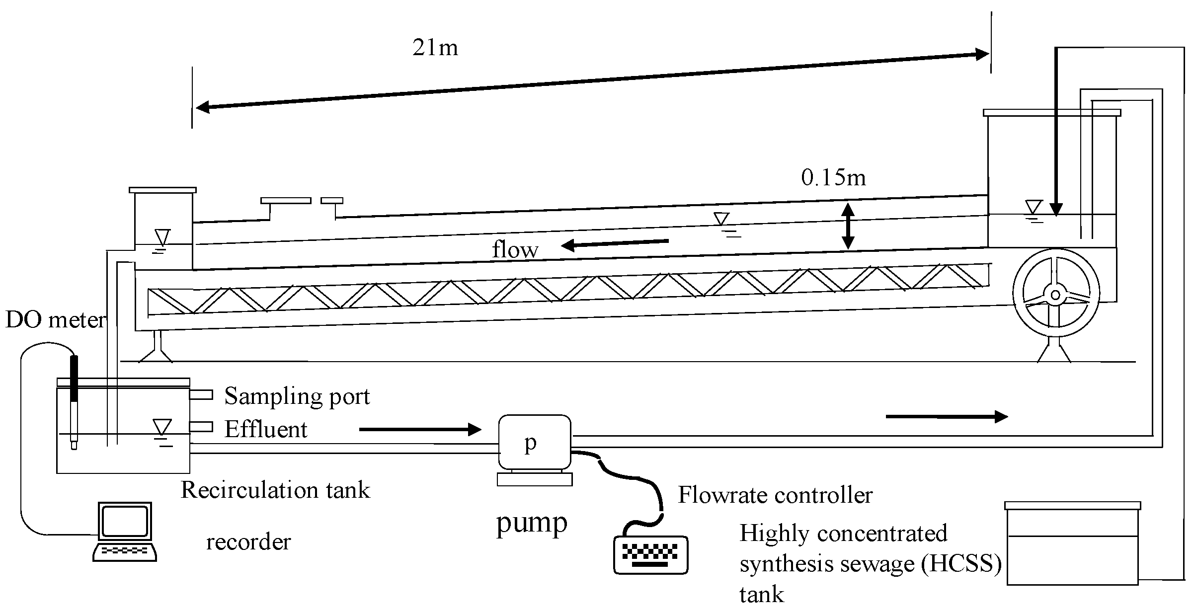
3.1. Pilot Sewer Pipe

A plastic pilot sewer pipe (PSP) 21 m long and 0.15 m in diameter was used for the experiments, as shown in Figure 1. The synthetic sewage flowrate and sewer pipe slope could be controlled. The synthetic sewage temperature in the PSP was controlled at 28 centigrade. The synthetic sewage in the tail tank could be conveyed to the head tank using a pump between these two water tanks. The DO concentration in the recirculation tank was monitored using a DO meter. All units including the pipe, highly concentrated synthesis sewage (HCSS) tank, head tank, recirculate tank, and tail tank were sealed to ensure the recirculated sewage was not being oxygenated.

3.2. Experiment Procedures

The HCSS was synthesized using milk powder, sucrose, acetates, and other reagents. For neutralization, a NaOH solution was adopted to control the pH of HCSS at 7–7.5.

Table 1. The compositions of highly concentrated synthetic sewage (HCSS).

Constituents *	Dosage (mg)
Full-fat dry milk powder	163.2
NH4Cl	40.0
Acetates	37.6
Urea	30.0
Sucrose	16.2
KH2PO4	15.0
FeCl3	0.1
NaOH	For neutralizing

* The constituents were dissolved in 1 L distilled water for synthetizing HCSS.

shows the major HCSS compositions. The HCSS was periodically added into the PSP at certain quantities to be mixed with the synthetic sewage in the PSP.

A certain amount of activated sludge was added into the PSP at a fixed influent flowrate. This demonstrated that the biofilm remained in a stable condition if the effluent concentration from the PSP revealed a constant value, i.e., the biofilm grew stably on the PSP bottom. When the batch experiment was finished, the biofilm was acclimated under a steady condition again. The steady flow velocity and the pH were controlled at 0.6 m s⁻¹ and 6.0–7.2, respectively. In the experiment, synthetic sewage of 500 mL was taken from the sampling port every 1 h and the concentrations of total chemical oxygen demand (COD), ammonia, nitrate, and DO were analyzed.

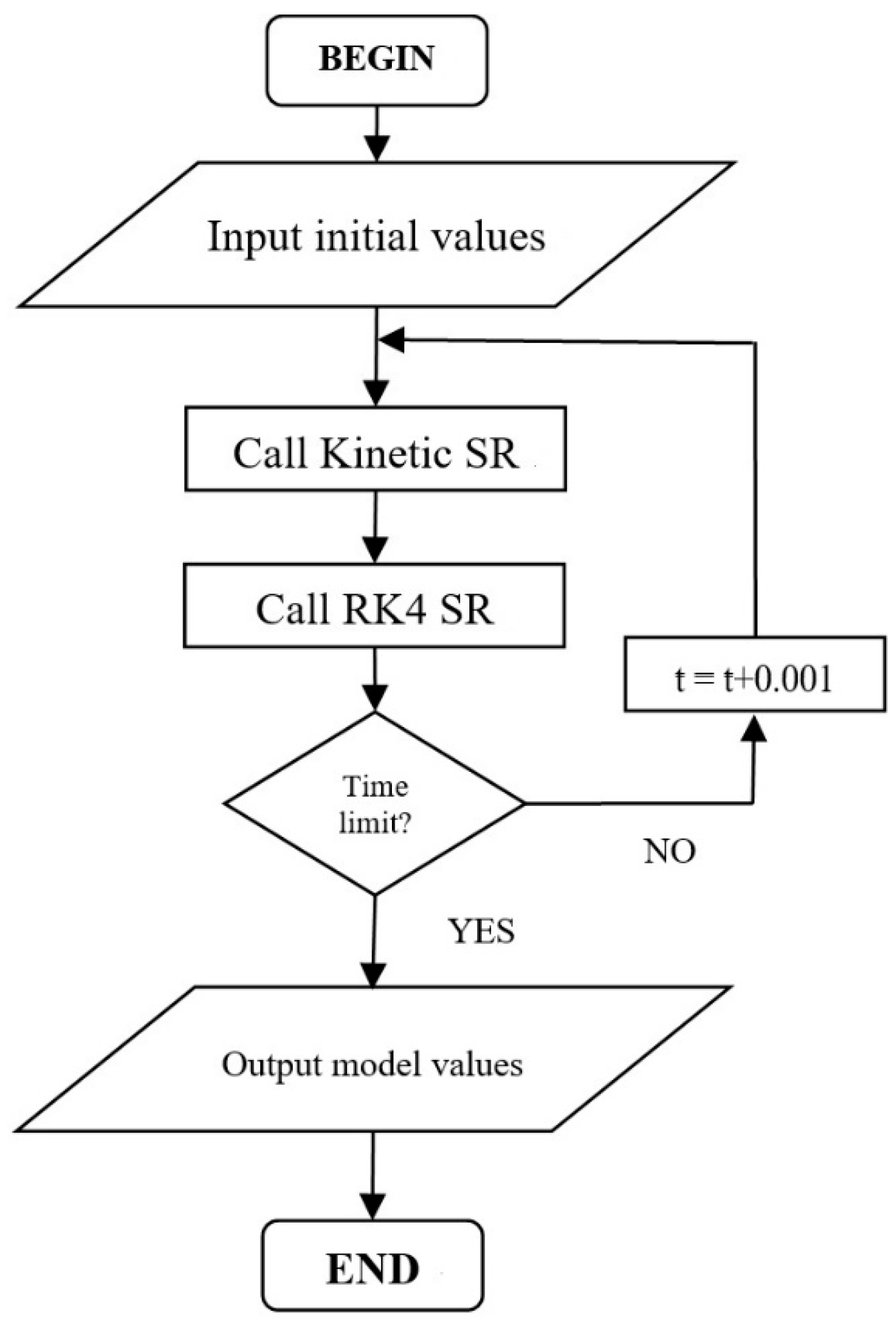
3.3. Establishment of SDM

When establishing the SDM, several kinetic reaction rate equations (RREs) from previous models were incorporated into GDM [5,6,7,11,12,13,14,18,19,20,21]. The GDM kinetics were only used in the simulation of the activated sludge process. In this study, the hydraulic condition was gravity flow in an open channel, neither completely mixing flow nor plug flow in the reactor. The active heterotrophic and autotrophic biomass was separated into two phases, i.e., the water phase and biofilm phase, in the open channel. Furthermore, the reaeration of oxygen in gravity flow was considered. Therefore, this study represents the first report of this innovative use of combined models to simulate the RRs of different compounds in the USP network. The stoichiometric constants and kinetic constants from previous models were also adopted [5,6,7,11,12,13,14,18,19,20,21].

Table 2. The definitions of compounds.

	Compounds and Definition	Unit
ZHW	Active heterotrophic biomass in the water phase	g COD m−3
ZHF	Active heterotrophic biomass in the biofilm	g COD m−3
ZAW	Active autotrophic biomass in the water phase	g COD m−3
ZAF	Active autotrophic biomass in the biofilm	g COD m−3
ZE	Endogenous mass	g COD m−3
SENM	Enmeshed slowly biodegradable substrates	g COD m−3
SBCS	Readily biodegradable “complex” substrate	g COD m−3
NBP	Particulate biodegradable organic nitrogen	g OrgN m−3
NBS	Soluble biodegradable organic nitrogen	g OrgN m−3
NH3	Ammonia-nitrogen	g NH3 m−3
NO3	Nitrate and nitrite nitrogen	g NO2− + NO3− m−3
SO2	Oxygen	g O2 m−3

shows the definitions of compounds in the established SDM. The RREs are shown in

Table 3. Symbols and definitions for reaction rate equations.

No.	Reaction	Equations
r1	Aerobic growth of ZHW in the water phase	μZHSBCS/(KS,ZH + SBCS)SO2/(KO,ZH + SO2)ZHWθW(T−20)
r2	Aerobic growth of ZHF in the biofilm	μZHSBCS/(KS,ZH + SBCS)SO2/(KO,ZH + SO2)εZHFθF(T−20)
r3	Anoxic growth of ZHW in the water phase	ηGROμZHSBCS/(KS,ZH + SBCS)KO,ZH/(KO,ZH + SO2)NO3/(KNO3 + NO3)ZHWθW(T−20)
r4	Anoxic growth of ZHF in the biofilm	ηGROμZHSBCS/(KS,ZH + SBCS)KO,ZH/(KO,ZH + SO2)NO3/(KNO3 + NO3)εZHFθF(T−20)
r5	Aerobic growth of ZAW in the water phase	μZANH3/(KNH3 + NH3)SO2/(KO,ZA + SO2)ZAWθW(T−20)
r6	Aerobic growth of ZAF in the biofilm	μZANH3/(KNH3 + NH3)SO2/(KO,ZA + SO2)εZAFθF(T−20)
r7	Organism decay of ZHW in the water phase	bZHZHWθW(T−20)
r8	Organism decay of ZHF in the biofilm	bZHZHFθF(T−20)
r9	Organism decay of ZAW in the water phase	bZAZAWθW(T−20)
r10	Organism decay of ZAF in the biofilm	bZAZAFθF(T−20)
r11	Ammonification of NBS	KRNBS(ZHWθW(T−20) + ZHFθF(T−20))
r12	Hydrolysis of SENM	KHSENM/(ZHWθW(T−20) + ZHFθF(T−20))/(KX + SENM/(ZHWθW(T−20) + ZHFθF(T−20)))(SO2/(KO,ZH + SO2)‡ + ηhKO,ZH/(KO,ZH + SO2)NO3/(KNO3 + NO3)) (ZHWθW(T−20) + ZHFθF(T−20))
r13	Hydrolysis of NBP	KHNBP/(ZHWθW(T−20) + ZHFθF(T−20))/(KX + SENM/(ZHWθW(T−20) + ZHFθF(T−20)))(SO2/(KO,ZH + SO2)‡ + ηhKO,ZH/(KO,ZH + SO2)NO3/(KNO3 + NO3))(ZHWθW(T−20) + ZHFθF(T−20))
r14	Reaeration of oxygen	KLa(SO2,SAT − SO2) where KLa = 0.96(1 + 0.2FR2)(SLOP·VM)3/8DH−1θR(T−20)

.

By combining the related constants and RREs in Table 3, the complete SDM for all types of compounds can be listed as follows:

$$\frac{d{Z}_{HW}}{dt}=r_1+r_3-r_7$$

(1)

$$\frac{d{Z}_{HF}}{dt}=r_2+r_4-r_8$$

(2)

$$\frac{d{Z}_{AW}}{dt}=r_5-r_9$$

(3)

$$\frac{d{Z}_{AF}}{dt}=r_6-r_{10}$$

(4)

$$\frac{d{Z}_E}{dt}=f_{ZE}\cdot r_7+f_{ZE}\cdot r_8+f_{ZE}\cdot r_9+f_{ZE}\cdot r_{10}$$

(5)

$$\frac{d{S}_{ENM}}{dt}=(1-f_{ZE})\cdot r_7+(1-f_{ZE})\cdot r_8+(1-f_{ZE})\cdot r_9+(1-f_{ZE})\cdot r_{10}-r_{12}$$

(6)

$$\frac{d{S}_{BCS}}{dt}=-\frac{1}{Y_{ZH}}\cdot r_1-\frac{1}{Y_{ZH}}\cdot r_2-\frac{1}{Y_{ZH}}\cdot r-\frac{1}{Y_{ZH}}\cdot r_4+r_{12}$$

(7)

$$\frac{d{N}_{H3}}{dt}=-f_{ZN}\cdot r_1-f_{ZN}\cdot r_2-f_{ZN}\cdot r_3-f_{ZN}\cdot r_4-(f_{ZN}+\frac{1}{Y_{ZA}})\cdot r_5-(f_{ZN}+\frac{1}{Y_{ZA}})\cdot r_6+r_{11}$$

(8)

$$\frac{d{N}_{O3}}{dt}=-\frac{1-Y_{ZH}}{2.86Y_{ZH}}\cdot r_3-\frac{1-Y_{ZH}}{2.86Y_{ZH}}\cdot r_4+\frac{1}{Y_{ZA}}\cdot r_5+\frac{1}{Y_{ZA}}\cdot r_6$$

(9)

$$\frac{d{N}_{BP}}{dt}=(f_{ZN}-f_{ZE}\cdot f_{ZNE})\cdot r_7+(f_{ZN}-f_{ZE}\cdot f_{ZNE})\cdot r_8+(f_{ZN}-f_{ZE}\cdot f_{ZNE})\cdot r_9+(f_{ZN}-f_{ZE}\cdot f_{ZNE})\cdot r_{10}-r_{13}$$

(10)

$$\frac{d{N}_{BS}}{dt}=-r_{11}+r_{13}$$

(11)

$$\frac{d{S}_{O2}}{dt}=-\frac{1-Y_{ZH}}{Y_{ZH}}\cdot r_1-\frac{1-Y_{ZH}}{Y_{ZH}}\cdot r_2-\frac{4.57-Y_{ZA}}{Y_{ZA}}\cdot r_5-\frac{4.57-Y_{ZA}}{Y_{ZA}}\cdot r_6+r_{14}$$

(12)

The values of relative constants for the established SDM are shown in

Table 4. Constant values.

Symbol	Definition	Value	Unit
μZH	Maximum specific growth rate for heterotrophs	6	day−1
bZH	Organism decay rate for heterotrophs	0.62	day−1
YZH	Yield for heterotrophs	0.67	g COD g−1 COD
KO,ZH	DO half-saturation constant for heterotrophs	0.2	g O2 m−3
KS,ZH	Half-saturation constant for heterotrophic growth	20	g COD m−3
KNO3	Nitrate half-saturation constant for denitrifying heterotrophs	0.5	g NO3-N m−3
ηGRO	Anoxic growth factor for μZH	0.8
μZA	Maximum specific growth rate for autotrophs	0.8	day−1
bZA	Organism decay rate for autotrophs	0.5	day−1
YZA	Yield for autotrophs	0.24	g COD g−1 COD
KO,ZA	DO half-saturation constant for autotrophs	0.4	g O2 m−3
KNH3	Half-saturation constant for autotrophic growth	1.0	g NH3-N m−3
KH	Maximum specific hydrolysis rate	3	day−1
KX	Half-Saturation constant for hydrolysis	0.03	g COD m−3
ηh	Anoxic factor for hydrolysis	0.4
KR	Ammonification rate	0.08	day−1
fZN	Nitrogen content of active mass	0.086
fZNE	Nitrogen content of endogenous mass	0.06
fZE	Fraction of active mass remaining as endogenous residue	0.08
ε	Efficiency constant in the biofilm	0.6
θW	Temperature constant in the water phase	1.07
θF	Temperature constant in the biofilm	1.03

. The flow conditions and reaeration effects are shown in

Table 5. Flow conditions and reaeration effect.

Symbol	Definition	Value	Unit
DH	Hydraulic mean depth	0.15	m
FR	Froude number = VM(g DH)−0.5	Calculated	--
KLa	Overall oxygen transfer constant	Calculated	day−1
g	Gravity acceleration	9.81	m s−2
SO2,SAT	Oxygen saturation concentration at T °C		g O2 m−3
SLOP	Slope of sewer pipe	0.01	mm−1
T	Temperature	20	°C
VM	Mean flow velocity	0.6	m s−1
θR	Temperature constant for reaeration	1.024	--

. The equation set from Equation (1) to Equation (12) formed an ordinary differential equation (ODE) system. The set of ODEs was then solved simultaneously using the subroutine (SB) of the fourth-order Runge–Kutta algorithm (RK4) [22]. The flow chart for the computer program is shown in Figure 2.

3.4. OURBE to Calculate Sensitive Constants and Initial Biomass

In the model, there were many kinetic constants. The oxygen uptake rate batch experiments (OURBE) adopted from our previous studies [23,24,25,26,27] were used to measure the sensitive kinetic constants including maximum specific growth rate for heterotrophs, organism decay rate for heterotrophs, maximum specific growth rate for autotrophs, organism decay rate for autotrophs, and initial biomass of heterotrophs (Z_H) and autotrophs (Z_A).

The OURBE equipment consisted of several tanks of fixed height and volume and magnetic stirrers for agitation and aeration. Highly stable oxygen meters connected to the data processer were adopted to measure DO. Since the OURBE equipment was sealed and airtight, the actual respiration rate of microorganisms at any time did not depend on oxygen input into OURBE. The actual oxygen uptake rate (OUR) values could be measured using the DO values. A certain amount of biofilm was sampled from the PSP and added into the OURBE equipment. Substrates containing glucose, NH₄SO₄, and KH₂PO₄ were added, resulting in a total volume of 1000 mL in the OURBE equipment, in which the pH value was controlled at 7. The OURBE equipment was periodically aerated to measure OUR. Furthermore, the kinetic constants and initial biomass of Z_H and Z_A could be measured [23,24,25,26,27].

For those constants that are nearly fixed values in domestic sewage, the default values from GDM and previous studies were used, as shown in Table 4 and Table 5 [5,6,11,12,13,14].

4. Results and Discussions

4.1. Experimental Results

In the PSP experiment, the volatile suspended solids (VSS) in the water phase were nearly 1.0 mg L⁻¹, so the Z_HW concentration was considered to be 1.0 mg L⁻¹. The autotrophs’ biomass could not be easily measured using OURBE because of their low concentration, so Z_AW was considered to be 0.0 mg L⁻¹. The values of Z_HF and Z_AF were approximately 400.0 and 0.1 mg L⁻¹ in accordance with OURBE. These values were close to those in our previous in situ survey [28]. The Standard Methods [29] were adopted to measure the concentrations of other compounds. Nitrogen compound concentrations (N_BP, N_SP, N_H3, and N_O3) ranged from 2.0 to 30.1 mg L⁻¹. According to the PSP experiments, the initial OVs for Z_HW, Z_HF, Z_AW, Z_AF, Z_E, S_ENM, S_BCS, N_BP, N_BS, N_H3, N_O3, and S_O2 were 1.0, 400.0, 0.0, 0.1, 1.0, 134.0, 281.0, 8.0, 30.1, 25.4, 2.0, and 6.2 mg L⁻¹, respectively. The OVs of different compounds at various flowing times are shown in Figure 3.

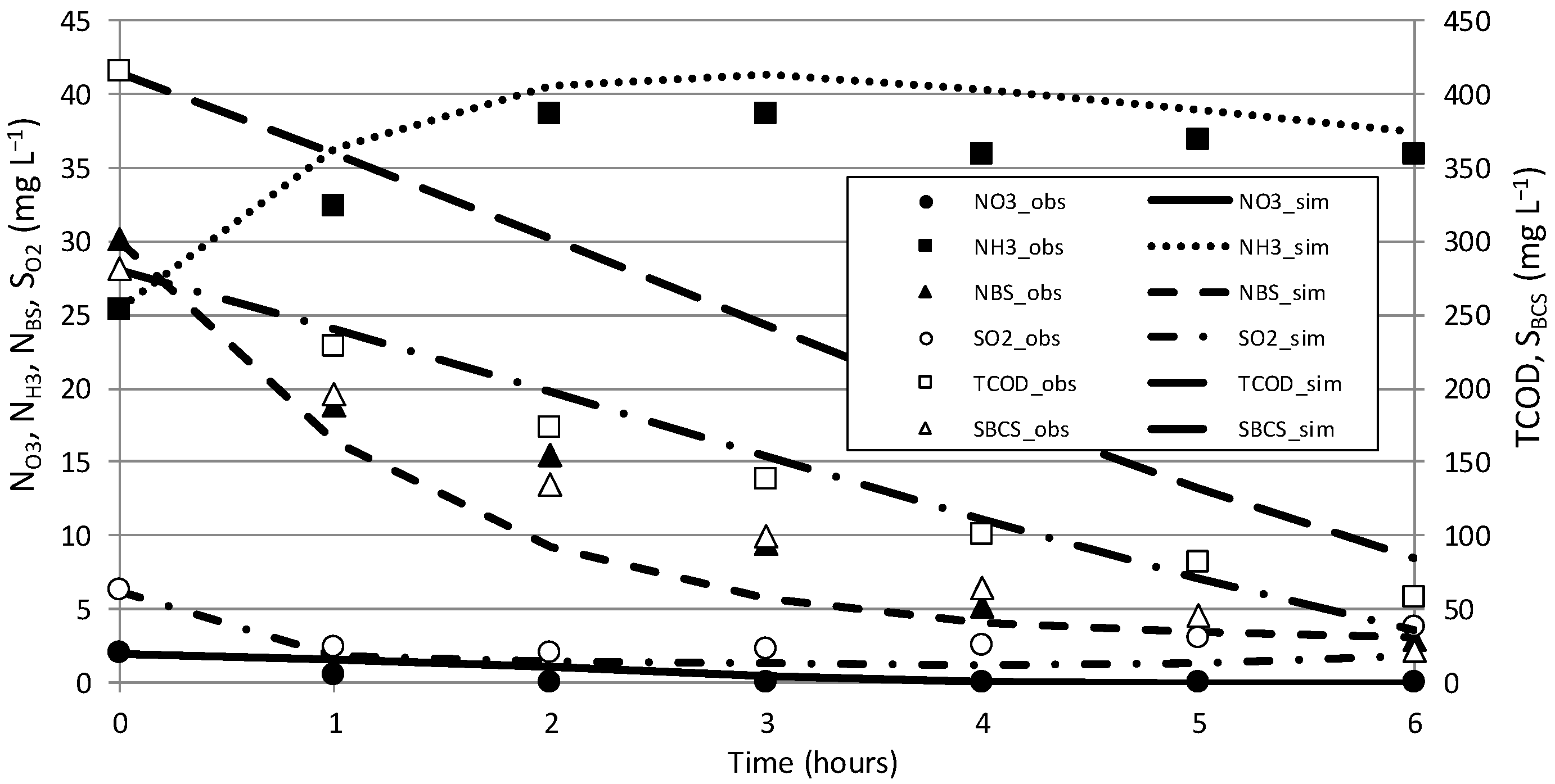
4.2. Model Validation

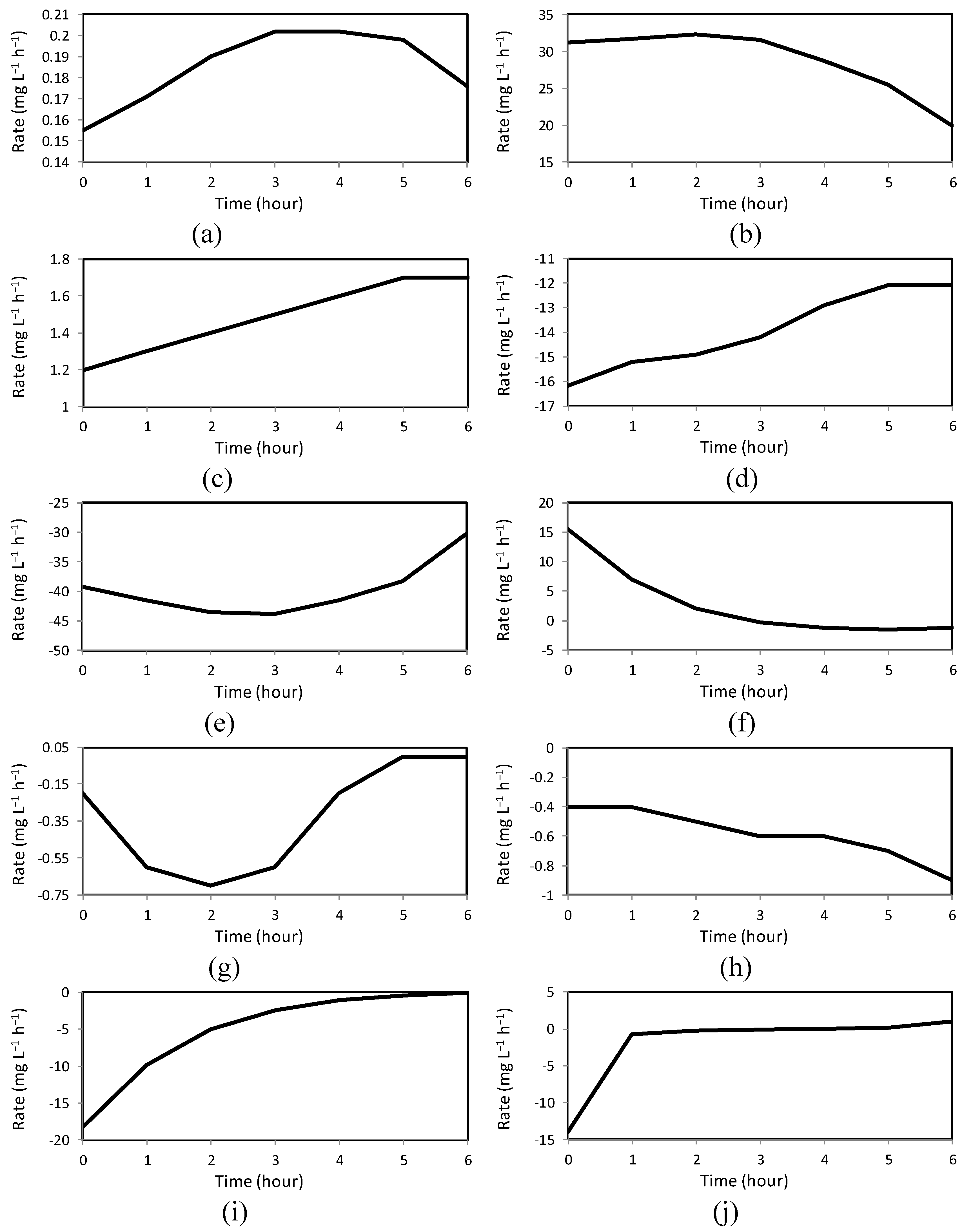
To verify the consistency between the SVs and OVs of different compounds in the water phase, the coefficient of determination (R²) and correlation coefficient (R) were used as follows [30]:

$$R^2=\frac{{\displaystyle \sum _{i=1}^n{\left(s{v}_i-\overline{ov}\right)}^2}}{{\displaystyle \sum _{i=1}^n{\left(s{v}_i-o{v}_i\right)}^2}+{\displaystyle \sum _{i=1}^n{\left(s{v}_i-\overline{ov}\right)}^2}}$$

(13)

$$R=\frac{{\displaystyle \sum _{i=1}^n(s{v}_i-\overline{sv})(o{v}_i-\overline{ov})}}{\sqrt{{{\displaystyle \sum _{i=1}^n(s{v}_i-\overline{sv})}}^2{{\displaystyle \sum _{i=1}^n(o{v}_i-\overline{ov})}}^2}}$$

(14)

where R² is the coefficient of determination, R is the correlation coefficient, sv is the SV, $\overline{sv}$ is the mean SV, ov is the OV, $\overline{ov}$ is the mean OV, and n is the number of concentrations. R² is used to explain how differences in OV can be explained by the difference in SV. It is represented as a value between 0.0 and 1.0. If the R² value is higher than 0.7, this value is generally considered as having a strong effect [30]. R is used to calculate the strength of the linear relationship between SV and OV. A value of R between 0.7 and 1.0 indicates a highly positive linear relationship. In this study, R² and R were used to justify whether SV and OV were consistent or not, providing a measure of how well OVs were replicated by the SDM model.

Figure 2 also shows the consistency between the SVs and OVs of selected compounds in the water phase. The R² values between SVs and OVs for S_BCS, N_O3, N_H3, N_SP, and S_O2 were 0.83, 0.70, 0.87, 0.91, and 0.73, respectively. The R values for those were 0.97, 0.81, 0.91, 0.97, and 0.93, respectively. These R² and R were greater than 0.7 and 0.81, respectively. According to the study proposed by Moore et al. [30], the SVs and OVs of the selected compounds were highly consistent.

4.3. RR of Z_HW

Since the established model was validated, the RRs of different compounds at different flowing times could be calculated. Figure 4 shows the calculated RRs within 6 h.

According to Equation (1), Z_HW would grow because of r₁ (aerobic growth of Z_HW in the water phase) and r₃ (anoxic growth of Z_HW in the water phase), and decay because of r₇ (organism decay of Z_HW in the water phase). In the simulation proposed by Tanaka and Hvitved-Jacobsen [31], Z_HW would grow from 32.0 to 35.0 mg L⁻¹ within the initial 4 h, revealing positive RRs.

In Figure 4a, the RR for Z_HW was 0.155 mg L⁻¹ h⁻¹ at the initial time, began to increase before the 3rd hour, and reached its highest value of 0.202 mg L⁻¹ h⁻¹ at the 3rd–4th hour, afterward the RR decreased gradually to a value of 0.176 mg L⁻¹ h⁻¹ at the 6th hour.

Before the 3rd hour, the r₁ (aerobic growth of Z_HW in the water phase) and r₃ (anoxic growth of Z_HW in the water phase) with positive signs were high because of high S_BCS as shown in Figure 3. Therefore, the sum for the growth rate of Z_HW (r₁ +r₃) was greater than r₇ (organism decay of Z_HW in the water phase) and the RRs began to increase before the 3rd hour. After the 4th hour, the sum for the growth rate of Z_HW (r₁ +r₃) was less than r₇ because the sum for the growth rate of Z_HW became lower. Therefore, the RRs revealed a decreasing trend after the 4th hour.

4.4. RR of Z_HF

According to Equation (2), Z_HF would grow because of r₂ (aerobic growth of Z_HF in the biofilm) and r₄ (anoxic growth of Z_HF in the biofilm), and decay because of r₈ (organism decay of Z_HF in the biofilm). According to a study by Nielsen et al. [32], the biofilms grew linearly at an average rate of 0.2 mm day⁻¹ thickness during a series of experiments, revealing positive RRs.

In Figure 4b, the rates of Z_HF were 31.2 mg L⁻¹ h⁻¹ at the initial time, began to increase before the 2nd hour, and reached the highest value of 32.3 mg L⁻¹ h⁻¹ at the 2nd hour, afterward, the RR decreased gradually to a value of 19.9 mg L⁻¹ h⁻¹ at the 6th hour.

Before the 2nd hour, the r₂ (aerobic growth of Z_HF in the biofilm) and r₄ (anoxic growth of Z_HF in the biofilm) with positive signs were high because of high S_BCS as shown in Figure 3. Therefore, the sum for the growth rate of Z_HF (r₂ + r₄) was greater than r₈ (organism decay of Z_HF in the biofilm) and the RRs began to increase before the 2nd hour. After the 2nd hour, the sum for the growth rate of Z_HF (r₂ + r₄) was less than r₈ because the sum for the growth rate of Z_HF became lower. Thus, the RRs revealed a decreasing trend after the 2nd hour.

4.5. RRs of Z_AW and Z_AF

According to Equation (3), Z_AW would grow because of r₅ (aerobic growth of Z_AW in the water phase) and decay because of r₉ (organism decay of Z_AW in the water phase). According to Equation (4), Z_AF would grow because of r₆ (aerobic growth of Z_AF in the biofilm) and decay because of r₁₀. In the experiment, the organism biomass of the autotrophs in the water phase was ignored. The value of Z_AF was about 0.1 mg L⁻¹ according to OURBE. The calculation indicated that the RRs of Z_AW and Z_AF were almost zero.

4.6. RR of Z_E

According to Equation (5), Z_E would increase because of r₇ (organism decay of Z_HW in the water phase), r₈ (organism decay of Z_HF in the biofilm), r₉ (organism decay of Z_AW in the water phase), and r₁₀ (organism decay of Z_AF in the biofilm).

In Figure 4c, the RR of Z_E was 1.2 mg L⁻¹ h⁻¹ at the initial time, began to increase, and reached the highest value of 1.7 mg L⁻¹ h⁻¹ at the 5th hour, afterward, the RR remained fixed at the value 1.7 mg L⁻¹ h⁻¹ at the 6th hour.

Before the 5th hour, the biomass of Z_HW, Z_HF, Z_AW, and Z_AF in r₇ (organism decay of Z_HW in the water phase), r₈ (organism decay of Z_HF in the biofilm), r₉ (organism decay of Z_AW in the water phase), and r₁₀ (organism decay of Z_AF in the biofilm) increased continuously. Thus, the RR of Z_E continuously increased before the 5th hour. After the 5th hour, the biomass for the organisms was more stable, so the RR remained fixed at the value of 1.7 mg L⁻¹ h⁻¹ at the 6th hour.

4.7. RR of S_ENM

According to Equation (6), S_ENM would be supplied because of r₇ (organism decay of Z_HW in the water phase), r₈ (organism decay of Z_HF in the biofilm), r₉ (organism decay of Z_AW in the water phase), and r₁₀ (organism decay of Z_AF in the biofilm), and consumed because of r₁₂ (hydrolysis of S_ENM). According to the simulation carried out by Vollertsen et al. [33], in which the maximum specific hydrolysis rate for S_ENM was 4.0 day⁻¹, the S_ENM was 40 mg L⁻¹ at the 0th km and 28 mg L⁻¹ at the 20th km, revealing significant biodegradation and negative RRs.

In Figure 4d, the RR of S_ENM was −16.2 mg L⁻¹ h⁻¹ at the initial time and increased gradually to a value of −12.1 mg L⁻¹ h⁻¹ at the 6th hour. During the whole experimental time of 6 h, the r₇ (organism decay of Z_HW in the water phase), r₈ (organism decay of Z_HF in the biofilm), r₉ (organism decay of Z_AW in the water phase), and r₁₀ (organism decay of Z_AF in the biofilm) with positive signs were low, but r₁₂ (hydrolysis of S_ENM) with a negative sign was relatively high. However, r₁₂ became lower because of decreasing S_ENM, so the RR of S_ENM increased gradually. It indicated that the supply rate of S_ENM was lower than the consumption rate in the experiment.

4.8. RR of S_BCS

According to Equation (7), S_BCS would be consumed because of r₁ (aerobic growth of Z_HW in the water phase), r₂ (aerobic growth of Z_HF in the biofilm), r₃ (anoxic growth of Z_HW in the water phase), and r₄ (anoxic growth of Z_HF in the biofilm), and supplied because of r₁₂ (hydrolysis of S_ENM). According to previous studies reported by Raunkjær et al. [34], the removal rate of S_BCS (acetate) was 4.13 g m⁻² h⁻¹ and 1.98 g m⁻² h⁻¹ under low-loaded and high-loaded conditions, respectively, revealing significant biodegradation. In the simulation proposed by Vollertsen et al. [33], the S_BCS was 30 mg L⁻¹ at the 0th km and 3 mg L⁻¹ at the 20th km, revealing significant biodegradation and negative RRs.

In Figure 4e, the RR of S_BCS was −39.2 mg L⁻¹ h⁻¹ at the initial time, began to decrease before the 3rd hour and reached the lowest value of −43.9 mg L⁻¹ h⁻¹ at the 3rd hour, afterward the RR increased gradually to a value of −30.2 mg L⁻¹ h⁻¹ at the 6th hour.

Before the 3rd hour, the r₁ (aerobic growth of Z_HW in the water phase), r₂ (aerobic growth of Z_HF in the biofilm), r₃ (anoxic growth of Z_HW in the water phase), and r₄ (anoxic growth of Z_HF in the biofilm) with negative signs were high because of high S_BCS, but r₁₂ (hydrolysis of S_ENM) with a positive sign was relatively low. After the 3rd hour, the sum for consumption rate of S_BCS (r₁ + r₂ + r₃ + r₄) became lower because of low S_BCS. So the RRs revealed an increasing trend after the 3rd hour. The RR of S_BCS was highly negative at the initial time and final time. It indicated that the supply rate of S_BCS was lower than the consumption rate in the experiment.

4.9. RR of N_H3

According to Equation (8), N_H3 would be consumed because of r₁ (aerobic growth of Z_HW in the water phase), r₂ (aerobic growth of Z_HF in the biofilm), r₃ (anoxic growth of Z_HW in the water phase), r₄ (anoxic growth of Z_HF in the biofilm), r₅ (aerobic growth of Z_AW in the water phase), and r₆ (aerobic growth of Z_AF in the biofilm), and supplied because of r₁₁ (ammonification of N_BS). In a study by Marjaka et al. [35], the removal of dissolved organic carbon and nitrogen in a USP with a fabricated porous ceramic bed was investigated. When N_H3 was used as the nitrogen source, and air was supplied through the aerator, 56% of the initial N_H3 was removed within 180 min. On the other hand, the value was about 38% when aeration was not applied. In their nitrification test, the RR of N_H3 was negative. But in our study, the RR of N_H3 was positive because of the hydrolysis of organic nitrogen.

In Figure 4f, the RR of N_H3 was 15.5 mg L⁻¹ h⁻¹ at the initial time, began to decrease before the 5th hour and reached the lowest value of −1.6 mg L⁻¹ h⁻¹ at the 5th hour, afterward, the RR increased slightly to a value of −1.2 mg L⁻¹ h⁻¹ at the 6th hour.

Before the 5th hour, the r₁ (aerobic growth of Z_HW in the water phase), r₂ (aerobic growth of Z_HF in the biofilm), r₃ (anoxic growth of Z_HW in the water phase), r₄ (anoxic growth of Z_HF in the biofilm), r₅ (aerobic growth of Z_AW in the water phase), and r₆ (aerobic growth of Z_AF in the biofilm) with negative signs decreased highly because of high N_H3, but r₁₁ (ammonification of N_BS) with a positive sign increased slightly. Thus, N_H3 decreased before the 5th hour.

It indicated that the supply rate of N_H3 was greater than the consumption rate at the initial time, but the supply rate was smaller than the consumption rate from 3rd hour in the experiment. The RR of N_H3 could be also regarded as the nitrification rate. Since the supply rate of N_H3 was greater than the consumption rate, the nitrification rate was not obvious. This is consistent with the results proposed by Shoji et al. [36], Liang et al. [37], and our previous in-situ study [28].

4.10. RR of N_O3

According to Equation (9), N_O3 would be consumed because of r₃ (anoxic growth of Z_HW in the water phase) and r₄ (anoxic growth of Z_HF in the biofilm), and supplied because of r₅ (aerobic growth of Z_AW in the water phase) and r₆ (aerobic growth of Z_AH in the biofilm). In the study proposed by Marjaka et al. [35], nitrite and nitrate concentrations in the nitrification test were low, indicating that the conversion of nitrite and nitrate to nitrogen gas by denitrification might undergo; therefore, the RR of N_O3 was negative. In the experiments carried out by Æsøy et al. [38], the denitrification rate of 3.5–4.3 g NO₃-N m⁻² day⁻¹ was observed in the PSP. This indicated the RR of N_O3 was negative in the PSP.

In Figure 4g, the RR of N_O3 was −0.2 mg L⁻¹ h⁻¹ at the initial time, began to decrease before the 2nd hour, reached the lowest value of −0.7 mg L⁻¹ h⁻¹ at the 2nd hour, afterward the RR increased gradually to a value of 0.0 mg L⁻¹ h⁻¹ at the 6th hour.

Before the 2nd hour, the r₃ (anoxic growth of Z_HW in the water phase) and r₄ (anoxic growth of Z_HF in the biofilm) with negative signs decreased highly, but r₅ (aerobic growth of Z_AW in the water phase) and r₆ (aerobic growth of Z_AH in the biofilm) with positive signs increased slightly. Thus, the RR of N_O3 decreased before the 2nd hour. After the 2nd hour, r₃ and r₄ became lower because of low N_O3. Therefore, the RRs revealed an increasing trend after the 2nd hour.

This indicated that the supply rate was smaller than the consumption rate in the experiment. The RR of N_O3 could be also be regarded as the denitrification rate. Denitrification did not occur obviously because of the low initial concentration and poor denitrification activity. This is consistent with the results proposed by Shoji et al. [36].

4.11. RR of N_BP

According to Equation (10), N_BP would be supplied because of r₇ (organism decay of Z_HW in the water phase), r₈ (organism decay of Z_HF in the biofilm), r₉ (organism decay of Z_AW in the water phase), and r₁₀ (organism decay of Z_AF in the biofilm), and consumed because of r₁₃ (hydrolysis of N_BP).

In Figure 4h, the RR of N_BP was −0.4 mg L⁻¹ h⁻¹ at the initial time and decreased gradually to a value of −0.9 mg L⁻¹ h⁻¹ at the 6th hour.

During the whole experimental time of 6 h, the r₇ (organism decay of Z_HW in the water phase), r₈ (organism decay of Z_HF in the biofilm), r₉ (organism decay of Z_AW in the water phase), and r₁₀ (organism decay of Z_AF in the biofilm) with positive signs were low, but r₁₃ (hydrolysis of N_BP) with a negative sign was relatively high. Therefore, the RR of N_BP decreased gradually to a value of −0.9 mg L⁻¹ h⁻¹ at the 6th hour. This indicated that the supply rate of N_BP was smaller than the consumption rate in the experiment.

4.12. RR of N_BS

According to Equation (11), N_BS would be consumed because of r₁₁ (ammonification of N_BS) and supplied because of r₁₃ (hydrolysis of N_BP).

In Figure 4i, the RR of N_BS was −18.3 mg L⁻¹ h⁻¹ at the initial time and increased gradually to a value of −0.1 mg L⁻¹ h⁻¹ at the 6th hour. During the whole experimental time of 6 h, the r₁₁ (ammonification of N_BS) with a negative sign was greater than r₁₃ (hydrolysis of N_BP) with a positive sign. Thus, the RR of N_BS increased gradually. It indicated that the supply rate was smaller than the consumption rate in the experiment.

4.13. RR of S_O2

According to Equation (12), S_O2 would be consumed because of r₁ (aerobic growth of Z_HW in the water phase), r₂ (aerobic growth of Z_HF in the biofilm), r₅ (aerobic growth of Z_AW in the water phase), and r₆ (aerobic growth of Z_AF in the biofilm), and supplied because of r₁₄ (reaeration of oxygen) [39]. In a study by Marjaka et al. [35], the S_O2 value was decreased to 2.0 mg L⁻¹ within the first 15 min, and then increased gradually to 6.0 mg L⁻¹ when organic carbon was almost completely consumed. When no aeration was applied, the S_O2 concentration decreased to 0.0 mg L⁻¹ within 30.0 min and an anaerobic condition was maintained until 120.0 min. Then S_O2 concentration gradually increased to 4.0 mg L⁻¹ during the rest period.

In Figure 4j, the RR of S_O2 was −14.0 mg L⁻¹ h⁻¹ at the initial time, 0.0 mg L⁻¹ h⁻¹ at the 4th hour, and 1.0 mg L⁻¹ h⁻¹ at the 6th hour, respectively.

According to Figure 3, S_O2 was 6.23 mg L⁻¹ at the initial time, began to decrease to the lowest value of 1.98 mg L⁻¹ at the 2nd hour, and then increased gradually to 3.76 mg L⁻¹ at the 6th hour. Therefore, the r₁ (aerobic growth of Z_HW in the water phase), r₂ (aerobic growth of Z_HF in the biofilm), r₅ (aerobic growth of Z_AW in the water phase), and r₆ (aerobic growth of Z_AF in the biofilm) with negative signs were greater than r₁₄ (reaeration of oxygen) with a positive sign before the 2nd hour. After the 2nd hour, r₁₄ (reaeration of oxygen) was greater than the sum of r₁, r₂, r₅, and r₆. Thus, the RR of S_O2 increased gradually to a value of 1.0 mg L⁻¹ h⁻¹ at the 6th hour.

This indicated that the supply rate was smaller than the consumption rate before the 4th hour because of significant organism activity, and, subsequently, the supply rate was greater than the consumption rate after the 4th hour because of reaeration.

5. Conclusions

The SDM, an innovative use of combined models, was established to describe the reaction of several compounds in the PSP. The established model was validated by calculating the consistency between the SVs and OVs of different compounds. R² and R were greater than 0.7 and 0.81, respectively, revealing that the SVs and OVs of selected compounds were highly consistent. Therefore, the RRs of compounds in the PSP were calculated using the SDM.

For Z_HW and Z_HF, their growth rates were greater than the organism decay rates in the experiment. For Z_E, S_ENM, S_BCS, N_O3, N_BP, and N_BS, their supply rate was smaller than the consumption rate in the experiment. For N_H3, the supply rate was greater than the consumption rate at the initial time, but the supply rate was smaller than the consumption rate from 3rd hour in the experiment. The supply rate of S_O2 was smaller than the consumption rate before the 4th hour because of significant microorganism activity, and, subsequently, the supply rate was greater than the consumption rate after the 4th hour because of reaeration. The kinetic constants and RREs in the SDM could be applied to predict the real-world situation.

6. Recommendations for Future Research

The results of this study not only provide an insight into the reaction rates of different compounds in the USP and an urban water network modeling reference for policymaking and regulation but also valuable data to help designers create more reasonable USP planning. However, in situ experiments in the USP are suggested to further explore the SDM in the future.

References

1. Tung, Y.T.; Pai, T.Y. Water management for agriculture, energy and social security in Taiwan. Clean (Weinh) 2015, 43, 627–632. [Google Scholar] [CrossRef]
2. Jiang, F.; Leung, D.H.; Li, S.; Chen, G.-H.; Okabe, S.; van Loosdrecht, M.C.M. A biofilm model for prediction of pollutant transformation in sewers. Water Res. 2009, 43, 3187–3198. [Google Scholar] [CrossRef]
3. Gao, J.; Li, J.; Jiang, G.; Shypanski, A.H.; Nieradzik, L.M.; Yuan, Z.; Mueller, J.F.; Ort, C.; Thai, P.K. Systematic evaluation of biomarker stability in pilot scale sewer pipes. Water Res. 2019, 151, 447–455. [Google Scholar] [CrossRef] [Green Version]
4. Nielsen, A.H.; Vollertsen, J. Model parameters for aerobic biological sulfide oxidation in sewer wastewater. Water 2021, 13, 981. [Google Scholar] [CrossRef]
5. Pai, T.Y.; Shyu, G.S.; Chen, L.; Lo, H.M.; Chang, D.H.; Lai, W.J.; Yang, P.Y.; Chen, C.Y.; Liao, Y.C.; Tseng, S.C. Modelling transportation and transformation of nitrogen compounds at different influent concentrations in sewer pipe. Appl. Math. Model. 2013, 37, 1553–1563. [Google Scholar] [CrossRef]
6. Pai, T.Y.; Wang, S.C.; Lo, H.M.; Chen, L.; Wan, T.J.; Lin, M.R.; Lin, C.Y.; Yang, P.Y.; Lai, W.J.; Wang, Y.H.; et al. A simulation of sewer biodeterioration by analysis of different components with a model approach. Int. Biodeterior. Biodegrad. 2017, 125, 37–44. [Google Scholar] [CrossRef]
7. Butler, D.; Friedler, E.; Gatt, K. Characterising the quantity and quality of domestic wastewater inflows. Water Sci. Technol. 1995, 31, 13–24. [Google Scholar] [CrossRef]
8. Short, M.D.; Peirson, W.L.; Peters, G.M.; Cox, R.J. Managing adaptation of urban water systems in a changing climate. Water Resour. Manag. 2012, 26, 1953–1981. [Google Scholar] [CrossRef]
9. Short, M.D.; Daikeler, A.; Peters, G.M.; Mann, K.; Ashbolt, N.J.; Stuetz, R.M.; Peirson, W.L. Municipal gravity sewers: An unrecognised source of nitrous oxide. Sci. Total Environ. 2014, 468–469, 211–218. [Google Scholar] [CrossRef]
10. Van de Walle, J.L.; Goetz, G.W.; Huse, S.M.; Morrison, H.G.; Sogin, M.L.; Hoffmann, R.G.; Yan, K.; McLellan, S.L. Acinetobacter, Aeromonas and Trichococcus populations dominate the microbial community within urban sewer infrastructure. Environ. Microbiol. 2012, 14, 2538–2552. [Google Scholar] [CrossRef] [PubMed]
11. Henze, M.; Gujer, W.; Mino, T.; van Loosdrecht, M.C.M. Activated Sludge Models: ASM1, ASM2, ASM2d and ASM3; International Water Association: London, UK, 2000. [Google Scholar]
12. Hvitved-Jacobsen, T.; Vollertsen, J.; Nielsen, P.H. A process and model concept for microbial wastewater transformations in gravity sewers. Water Sci. Technol. 1998, 37, 233–241. [Google Scholar] [CrossRef]
13. Hvitved-Jacobsen, T.; Vollertsen, J.; Tanaka, N. Wastewater quality changes during transport in sewers-an integrated aerobic and anaerobic model concept for carbon and sulfur microbial transformations. Water Sci. Technol. 1998, 38, 257–264. [Google Scholar] [CrossRef]
14. Vollertsen, J.; Hvitved-Jacobsen, T. Aerobic microbial transformations of resuspended sediments in combined sewers–a conceptual model. Water Sci. Technol. 1998, 37, 69–76. [Google Scholar] [CrossRef]
15. Dittmer, U.; Bachmann-Machnik, A.; Launay, M.A. Impact of combined sewer systems on the quality of urban streams: Frequency and duration of elevated micropollutant concentrations. Water 2020, 12, 850. [Google Scholar] [CrossRef] [Green Version]
16. Langeveld, J.; van Daal, P.; Schilperoort, R.; Nopens, I.; Flameling, T.; Weijers, S. Empirical sewer water quality model for generating influent data for WWTP modelling. Water 2017, 9, 491. [Google Scholar] [CrossRef] [Green Version]
17. Pai, T.Y.; Chuang, S.H.; Tsai, Y.P.; Ouyang, C.F. Modelling a combined anaerobic/anoxic oxide and rotating biological contactors process under dissolved oxygen variation by using an activated sludge-biofilm hybrid model. J. Environ. Eng. 2004, 130, 1433–1441. [Google Scholar] [CrossRef]
18. Pai, T.Y.; Ouyang, C.F.; Su, J.L.; Leu, H.G. Modelling the steady-state effluent characteristics of the TNCU process under different return mixed liquid. Appl. Math. Model. 2001, 25, 1025–1038. [Google Scholar] [CrossRef]
19. Pai, T.Y.; Tsai, Y.P.; Chou, Y.J.; Chang, H.Y.; Leu, H.G.; Ouyang, C.F. Microbial kinetic analysis of three different types of EBNR process. Chemosphere 2004, 55, 109–118. [Google Scholar] [CrossRef] [PubMed]
20. Pai, T.Y. Modeling nitrite and nitrate variations in A2O process under different return oxic mixed liquid using an extended model. Process. Biochem. 2007, 42, 978–987. [Google Scholar] [CrossRef]
21. Pai, T.Y.; Chang, H.Y.; Wan, T.J.; Chuang, S.H.; Tsai, Y.P. Using an extended activated sludge model to simulate nitrite and nitrate variations in TNCU2 process. Appl. Math. Model. 2009, 33, 4259–4268. [Google Scholar] [CrossRef]
22. Gerald, C.F.; Wheatley, P.O. Applied Numerical Analysis, 4th ed.; Addison-Wesley Publishing Company Inc.: New York, NY, USA, 1989. [Google Scholar]
23. Pai, T.Y.; Wang, S.C.; Lo, H.M.; Chiang, C.F.; Liu, M.H.; Chiou, R.J.; Chen, W.Y.; Hung, P.S.; Liao, W.C.; Leu, H.G. Novel modeling concept for evaluating the effects of cadmium and copper on heterotrophic growth and lysis rates in activated sludge process. J. Hazard. Mater. 2009, 166, 200–206. [Google Scholar] [CrossRef] [PubMed]
24. Pai, T.Y.; Wang, S.C.; Lin, C.Y.; Liao, W.C.; Chu, H.H.; Lin, T.S.; Liu, C.C.; Lin, S.W. Two types of organophosphate pesticides and their combined effects on heterotrophic growth rates in activated sludge process. J. Chem. Technol. Biotechnol. 2009, 84, 1773–1779. [Google Scholar] [CrossRef]
25. Pai, T.Y.; Wan, T.J.; Tsai, Y.P.; Tzeng, C.J.; Chu, H.H.; Tsai, Y.S.; Lin, C.Y. Effect of sludge retention time on nitrifiers’ biomass and kinetics in an anaerobic/oxic process. Clean 2010, 38, 167–172. [Google Scholar] [CrossRef]
26. Pai, T.Y.; Chiou, R.J.; Tzeng, C.J.; Lin, T.S.; Yeh, S.C.; Sung, P.J.; Tseng, C.H.; Tsai, C.H.; Tsai, Y.S.; Hsu, W.J.; et al. Variation of biomass and kinetic parameter for nitrifying species in TNCU3 process at different aerobic hydraulic retention time. World J. Microbiol. Biotechnol. 2010, 26, 589–597. [Google Scholar] [CrossRef]
27. Pai, T.Y.; Lo, H.M.; Wan, T.J.; Wang, S.C.; Yang, P.Y.; Huang, Y.T. Behaviors of biomass and kinetic parameter for nitrifying species in A2O process at different sludge retention time. Appl. Biochem. Biotechnol. 2014, 174, 2875–2885. [Google Scholar] [CrossRef] [PubMed]
28. Pai, T.Y.; Chen, C.L.; Chung, H.; Ho, H.H.; Shiu, T.W. Monitoring and assessing variation of sewage quality and microbial functional groups in a trunk sewer line. Environ. Monit. Assess. 2010, 171, 551–560. [Google Scholar] [CrossRef]
29. APHA; AWWA; WEF. Standard Methods for the Examination of Water and Wastewater, 20th ed.; American Public Health Association, American Water Works Association and Water Environment Federation: Washington, DC, USA, 1998. [Google Scholar]
30. Moore, D.S.; Notz, W.I.; Flinger, M.A. The Basic Practice of Statistics, 6th ed.; W.H. Freeman and Company: New York, NY, USA, 2013. [Google Scholar]
31. Tanaka, N.; Hvitved-Jacobsen, T. Transformations of wastewater organic matter in sewers under changing aerobic/anaerobic conditions. Water Sci. Technol. 1998, 37, 105–113. [Google Scholar] [CrossRef]
32. Nielsen, A.H.; Hvitved-Jacobsen, T.; Vollertsen, J. Kinetics and stoichiometry of sulfide oxidation by sewer biofilms. Water Res. 2005, 39, 4119–4125. [Google Scholar] [CrossRef] [PubMed]
33. Vollertsen, J.; Hvitved-Jacobsen, T.; McGregor, I.; Ashley, R. Aerobic microbial transformations of pipe and silt trap sediments from combined sewers. Water Sci. Technol. 1999, 39, 233–249. [Google Scholar] [CrossRef]
34. Raunkjær, K.; Nielsen, P.H.; Hvitved-Jacobsen, T. Acetate removal in sewer biofilms under aerobic conditions. Water Res. 1997, 31, 2727–2736. [Google Scholar] [CrossRef]
35. Marjaka, I.W.; Miyanaga, K.; Hori, K.; Tanji, Y.; Unno, H. Augmentation of self-purification capacity of sewer pipe by immobilizing microbes on the pipe surface. Biochem. Eng. J. 2003, 15, 69–75. [Google Scholar] [CrossRef] [Green Version]
36. Shoji, T.; Matsubara, Y.; Tamaki, S.; Matsuzaka, K.; Satoh, H.; Mino, T. In-sewer treatment system of enhancing self-purification: Performance and oxygen balance in pilot tests. J. Water Environ. Technol. 2015, 13, 427–439. [Google Scholar] [CrossRef]
37. Liang, Z.S.; Zhang, L.; Wu, D.; Chen, G.H.; Jiang, F. Systematic evaluation of a dynamic sewer process model for prediction of odor formation and mitigation in large-scale pressurized sewers in Hong Kong. Water Res. 2019, 154, 94–103. [Google Scholar] [CrossRef] [PubMed]
38. Æsøy, A.; Storfjell, M.; Mellgren, L.; Helness, H.; Thorvaldsen, G.; Ødegaard, H.; Bentzen, G. A comparison of biofilm growth and water quality changes in sewers with anoxic and anaerobic (septic) conditions. Water Sci. Technol. 1997, 36, 303–310. [Google Scholar] [CrossRef]
39. Pai, T.Y.; Ouyang, C.F.; Liao, Y.C.; Leu, H.G. Oxygen transfer in gravity flow sewer. Water Sci. Technol. 2000, 42, 417–422. [Google Scholar] [CrossRef] [Green Version]
Figure 1. Pilot sewer pipe.
Water 13 01580 g001
Figure 2. Computer program flow chart.
Water 13 01580 g002
Figure 3. The OVs of different compounds.
Water 13 01580 g003
Figure 4. The RRs of different compounds at different flowing times. (a) ZHW, (b) ZHF, (c) ZE, (d) SENM, (e) SBCS, (f) NH3, (g) NO3, (h) NBP, (i) NBS, and (j) SO2.
Water 13 01580 g004