Modelling Freshwater Eutrophication with Limited Limnological Data Using Artificial Neural Networks

Abstract

Artificial Neural Networks (ANNs) have wide applications in aquatic ecology and specifically in modelling water quality and biotic responses to environmental predictors. However, data scarcity is a common problem that raises the need to optimize modelling approaches to overcome data limitations. With this paper, we investigate the optimal k-fold cross validation in building an ANN using a small water-quality data set. The ANN was created to model the chlorophyll-a levels of a shallow eutrophic lake (Mikri Prespa) located in N. Greece. The typical water quality parameters serving as the ANN’s inputs are pH, dissolved oxygen, water temperature, phosphorus, nitrogen, electric conductivity, and Secchi disk depth. The available data set was small, containing only 89 data samples. For that reason, k-fold cross validation was used for training the ANN. To find the optimal k value for the k-fold cross validation, several values of k were tested (ranging from 3 to 30). Additionally, the leave-one-out (LOO) cross validation, which is an extreme case of the k-fold cross validation, was also applied. The ANN’s performance indices showed a clear trend to be improved as the k number was increased, while the best results were calculated for the LOO cross validation as expected. The computational times were calculated for each k value, where it was found the computational time is relatively low when applying the more expensive LOO cross validation; therefore, the LOO is recommended. Finally, a sensitivity analysis was examined using the ANN to investigate the interactions of the input parameters with the Chlorophyll-a, and hence examining the potential use of the ANN as a water management tool for nutrient control.

1. Introduction

Data-driven models are systematically used in the field of water resources management because they are less demanding in terms of data acquisition and quantity than the empirical and the physical-based hydrological models [1]. Artificial Neural Networks (ANNs) are such data-driven models with a wide application in water resources and aquatic sciences [2]. In particular, ANNs are used for modelling several domains of aquatic ecology such as benthic macroinvertebrates, planktonic communities, fish assemblages, and biomanipulation assessment [3]. During the last two decades, several ANN water quality modelling studies were performed with very good modelling results [4,5,6]. Their main advantages include their ability to model complex and nonlinear processes and the fact that they do not require assumptions about the distribution of the data or the relationships between input and output variables [2]. In addition, they offer the user the flexibility to successfully model environmental relationships with limited knowledge of the problem [7]. Thus, ANNs are considered ideal for modelling aquatic ecosystems, which are characterized by complex dynamics and nonlinear analytics [3].

Water quality monitoring programmes in particular produce a large amount of data with complex structures [8]. Unfortunately, there are also many cases where insufficient data quantity and quality can be a problem in ecological quality assessment and management [9]. Several factors such as bad weather conditions during monitoring, lack of funding, and problematic sensors are responsible for the lack of data. Data scarcity of water resources is an issue highlighted in the study of Cigizoglu and Kisi [10]; the authors address this issue successfully by applying k-fold cross validation into the ANN’s training data set. Generally, the phenomenon of data scarcity/small data sets when modelling with ANNs is an issue found in many scientific fields and the method of k-fold cross validation is widely used [11]. The problem of having a small data set when applying k-fold cross validation is discussed in a water quality modelling study of Goethals et al. [5], where it is stated that lower k-values may produce more robust ANN models, but with lower performance, and therefore a high k-value is recommended.

In this article, we address the issue of training an ANN with a small dataset of water quality parameters collected from a eutrophic lake in Greece. Eutrophication is one of the most significant problems today that is responsible for the degradation of water quality in many freshwater, coastal, and marine ecosystems worldwide [12,13]. Because freshwater lakes are major providers of ecosystem services (e.g., water supply for potable use and irrigation), eutrophication has severe socioeconomic implications that threaten human well-being, particularly in areas of the world where water is scarce. Therefore, scientists are developing new tools and methods for efficient and improved monitoring of water quality. In addition, they employ advanced modelling techniques and algorithms for creating novel forecasting schemes of eutrophication, since a lake’s ecosystem is very complex and sensitive and even a mild external pressure (such as tourist activity) with small inflows of biogenic elements can promote eutrophication [14]. Not surprisingly, ANNs have been used before in modelling eutrophication processes in lakes [15]. Linear regression methods and decision tree methods are some alternative methodologies used for eutrophication modelling. These methodologies have the merits of needing few parameters to adjust and being simple; however, they might not perform well when the data sample is small or does not follow certain assumptions about linear or Gaussian distributions [16]. In contrast, ANN models are not affected by the non-linearity effect, which is often observed between the environmental parameters associated with eutrophication [17].

The purpose of this modelling study is two-fold. First, we trained an ANN by implementing an approach of k-fold cross validation. Then, we compared the obtained modelling results between models built with different k values. Additionally, the factor of the needed computational time was also taken into consideration as a criterion for choosing the optimal model, with respect to the ANN performance and complexity in terms of computation time. Second, we examined the explanatory power of the optimal model to identify whether it can act as a water management tool. We show that the ANN managed to predict the chlorophyll-a levels of Lake Mikri Prespa with high accuracy. Based on this model, the contribution of each environmental parameter was evaluated with the use of a sensitivity analysis algorithm. The results of the sensitivity analysis produced useful conclusions about the role of each parameter with emphasis on the role of nutrients levels changes on the trophic status of the lake.

2. Materials and Methods

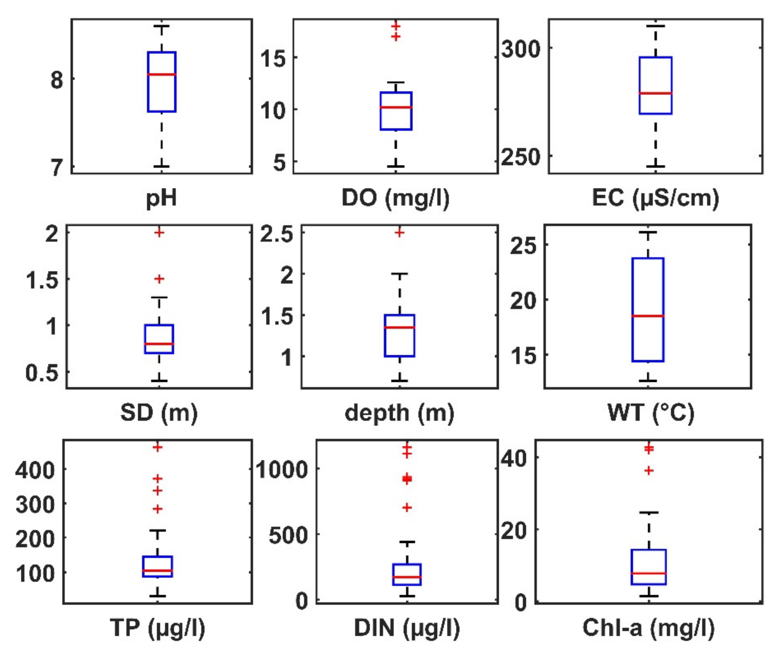
2.1. Study Area and Data Collection

The used dataset contains environmental variables obtained from Lake Mikri Prespa, a shallow eutrophic lake located in northwestern Greece. The lake is an ecosystem of great ecological importance as it belongs to the Prespa National park, is a Ramsar wetland site, an important bird area, and a Natura 2000 site [18]. The lake lies at an elevation of 853 m above sea level [19] and is located in the wider transboundary Prespa area shared by Greece, Albania, and North Macedonia (Figure 1). The climate of the area is characterized as sub-Mediterranean with continental influences, with frequent snowfall in the winter and summer rain drops [20]. The lake is characterized as a shallow lake, with approximately 48 km² of surface area, a maximum water depth of 8 m [21] and mean depth of 4.1 m [19]. The trophic status of the lake is characterized as eutrophic. As a result, prolonged cyanobacterial blooms have been recorded, which may start in spring and persist until December [22].

Chlorophyll-a concentration and environmental data were collected from fifteen sampling sites on a seasonal basis from 2006 to 2008 (see Hadjisolomou et al. [19]). We used the following environmental parameters as predictors of chlorophyll-a (Chl-a): pH, surface dissolved oxygen concentration (DO), electrical conductivity (EC), Secchi disk depth (SD), water depth (WD), surface water temperature (WT), total phosphorus concentration (TP) and dissolved inorganic nitrogen concentration (DIN).

The basic statistical properties of the environmental parameters are shown with the use of box plots in Figure 2.

2.2. Preliminaries on ANN and Model Construction

ANNs mimic the way biological neurons learn and make logical conclusions. A very popular ANN is the multi-layer feedforward (MLF) network trained by the backpropagation algorithm [23]. Feedforward networks are considered suitable for function approximation problems. The MLF networks are divided into at least three layers and each layer consists of neurons. The first layer is the input layer, followed by at least one intermediate hidden layer and the output layer that produces the final output. Each neuron of a layer relates to all the neurons of the next layer using synaptic weights. Every neuron performs aggregation on its weighted inputs and yields an output through an activation function. The most commonly used activation functions are the linear, the logistic and the hyperbolic tangent activation function [24]. The output value of the $j$-th neuron ($o_j$) is given by the equations as described by Dedecker et al. [25]:

$$o_j=f\left(u_j\right)$$

(1)

$$u_j={\displaystyle \sum }_{\forall i}{w}_{ij}{x}_i+z_j$$

(2)

where $f$ is the activation function, $x_i$ is the input from $i$-th neuron belonging to the immediate previous layer, $w_{ij}$ is the synaptic weight that connects $x_i$ with the $j$-th neuron and $z_j$ a bias term. The output of each neuron is computed and propagated through the next layer until the last layer, producing a network output that compares with the given output [26]. The learning procedure is repeated several times with the use of a training algorithm and each time the synaptic weights are adjusted until they minimize an error function, usually taken as the mean square difference between the predicted and the given output [27]. The Levenberg–Marquardt (LM) algorithm has the fastest convergence among the existing variations of backpropagation algorithms when it comes to ANNs with up to a few hundred parameters [23].

The topology of an ANN that determines the number of hidden layers and the number of neurons in each layer can be determined after a trial and error procedure [28,29]. The topology of a 3-layer ANN can be presented as L1-H1-L2 where L1 is the number of neurons in the input layer, H1 the number of neurons in the hidden layer and L2 the number of neurons in the output layer. In order to avoid overfitting, the maximum number of the hidden layer neurons can be computed according to the following the rule of thumb proposed by Maier et al. [30]:

$$N^H\le 2N^I+1$$

(3)

$$N^H\le 2N^{TR}/\left(N^I+1\right)$$

(4)

where $N^H$ is the number of hidden layer neurons, $N^I$ the number of inputs, and $N^{TR}$ the number of training samples. The maximum $N^H$ must be the smallest number found by those two rules.

Data normalization is a common procedure since the ANN’s performance is improved [25,31] and after network training the data is set back to its initial form. Dimensionality reduction of the measured variables is also recommended in order to achieve a reduced size of the original data set of variables [32]. The variable/parameter’s dimension reduction is performed not only because it reduces the model computational complexity, but also eliminates the possibility for model’s misconvergence and poor accuracy [4]. ANNs are evaluated based on several performance indices for their test set [33]. The Root Mean Square Error (RMSE) and Mean Absolute Error (MAE) are some commonly used performance indices and have the following mathematical formulas, respectively [34,35]:

$$RMSE=\sqrt{\frac{{{\displaystyle \sum }}_{i=1}^n{\left(o_i-s_i\right)}^2}{n}}$$

(5)

$$MAE=\frac{1}{n}{\displaystyle \sum }_{i=1}^n\left|o_i-s_i\right|$$

(6)

where for the above set of equations the parameter $o_i$ is the observed value, $s_i$ the simulated/predicted value, and $n$ the number of observations.

The sensitivity analysis is performed based on the ‘Perturb’ method. The ‘Perturb’ method is a sensitivity analysis methodology, which is computing the perturbation effect of the input variables regarding the output variable. The ‘Perturb’ method is examining the effect that a small change of an input variable has on the ANN’s output, therefore the input variables can be classified by an order of importance [36]. The mathematical formula that describes the ‘Perturb’ method of sensitivity analysis is explained by Lee et al. [37] as follows:

$$\mathrm{Sensitivity} \left(\%\right)=\frac{1}{n}{\displaystyle \sum }_{i=1}^n{\left(\frac{\mathrm{change} \mathrm{in} \mathrm{output} \left(\%\right)}{\mathrm{change} \mathrm{in} \mathrm{input} \left(\%\right)}\right)}_i\times 100$$

(7)

where $n$ represents the number of observations.

The k-fold cross validation method is used in order to avoid overfitting and the data set is divided into k equally sized folds/subsamples [38]. For each k-fold of the data set, an ANN model is trained on the other k − 1 folds of the data set and validated for the k-th fold. The cross-validation procedure is repeated k times (hence, each fold is used exactly once as the validation data set) and finally the average of the k calculated validation performance indices is computed [39,40]. According to Goethals et al. [5], the optimal k-value is found based on an evaluation procedure, where the robustness and reliability of the developed ANN models is assessed. A high value of k is recommended when the dataset is small and has very few observations. An extreme case of the k-fold cross validation method is the case of leave-one-out (LOO) cross validation, when the arithmetic value of k equals the number of measured samples (n) in the dataset.

3. Results

The monitored variables (pH, DO, EC, SD, depth, WT, TP, DIN, and Chl-a) were analyzed for collinearity by calculating the Pearson correlation coefficient (r). As stated by Gebler et al. [41], the deletion of the collinear parameters helps the ANN to avoid unnecessary/superfluous information and simplifies the model’s structure. The results of the correlation analysis (

Table 1. Results of the Pearson correlation coefficient (r) for the monitored environmental parameters.

	pH	DO	EC	SD	Depth	WT	TP	DIN	Chl-a
pH	1.000
DO	0.089	1.000
EC	0.260	−0.169	1.000
SD	−0.385	−0.229	0.094	1.000
depth	−0.153	−0.186	0.051	0.722	1.000
WT	0.442	−0.077	0.602	−0.278	−0.006	1.000
TP	−0.106	−0.164	0.048	0.299	0.216	−0.066	1.000
DIN	−0.131	0.251	0.097	0.059	−0.093	−0.179	0.198	1.000
Chl-a	0.234	−0.101	0.267	−0.124	−0.163	0.362	−0.014	−0.172	1.000

DO (dissolved oxygen, mg/L); EC (electric conductivity μS/cm); SD (Secchi disk, m) depth; depth (water depth, m); WT (water temperature, °C); TP (total phosphorus, μg/L); DIN (dissolved inorganic nitrogen, μg/L); Chl-a (Chlorophyll-a, mg/L). For strong correlations (r > 0.7), the associated value is shown with bold characters.

) revealed a strong correlation between the parameters SD depth and water depth ($r=0.722$). Therefore, the parameter water depth is eliminated from the ANN’s inputs. The Matlab (R2018b) software was used for data analysis and ANNs’ development for the needs of this study.

Several topologies were examined using a typical trial-and-error methodology, as recommended by Ozesmi et al. [29] and Palani et al. [42]; while a more analytical procedure for finding the ANN’s optimal topology is described in the study of Tuhtan et al. [43]. The 7-8-1 topology was found to be the optimal based on the calculated performance indices, which in our case are the Root Mean Square Error (RMSE) and the Mean Absolute Error (MAE). The k-fold cross validation method is applied in this modeling study, since the data sample for the ANN learning and training is small (n = 89, corresponding to sample points without any missing values). The optimal k-value was calculated among a candidate set for k values ranging between [3,30] and the LOO cross validation case (where k = 89). For each k-value, k ANNs (with the same topology 7-8-1) were created and their performance indices for the test sets were averaged (see Figure 3 and Figure 4). Based on RMSE and MAE results for each k-value, it was calculated that the optimal k-value was k = 89 since it produced the lowest RMSE and MAE. The calculated RMSE and MAE values for k = 89 are always equal because there is only one observation ($n=1$) per test data set (recall Equations (5) and (6)). It must also be noted that k = 89 exhibits the maximum number of outliers when calculating the RMSE and MAE performance indices. However, the ratio of outlier number per k-fold number (when k = 89) is lower than the calculated ratio for the majority of k = 3:30.

The computational time needed to train and test each ANN model for the different given k values was recorded (Figure 5). Based on the different time values that are needed for each k-fold, the comparison for the needed time and the ANN’s performance for the given k values is enabled (by observing Figure 3, Figure 4 and Figure 5). The LOO case had the highest computational time (t = 314 s), as expected. Even though the LOO case had the highest computational time, this time value is relatively low because the data set is small and consists of only 89 samples. The RMSE and MAE values are following a clear pattern, where they decrease as the k number increases. For the k = 89 case, the RMSE and MAE are equal to 0.36; however, for k = 30 the RMSE = 2.33 and MAE = 1.42. Therefore, for the k = 89 value there is a significant improvement of the ANN’s modelling performance compared with that of k = 30 with low computational overhead. So, by considering both the computational times and the performance indices, it is decided that the k = 89 (LOO) is the best value for the modelling needs of this study.

The associated results for predicting Lake’s Mikri Prespa Chl-a production are based on the averaged values for the LOO case. The ANN model’s sensitivity analysis is also expressed based on these averaged values.

The created ANN model managed to predict with good accuracy the Chl-a levels, as it was demonstrated from the RMSE and MAE indices. The measured values of the Chl-a parameter are plotted against those predicted by the ANN (Figure 6) for both the test dataset and the averaged predicted values of the entire dataset. It can be observed that these three graphical plots are almost identical. Therefore, the ANN model can be characterized as a reliable predictor for the Chl-a parameter. The biggest differences between the real and the averaged predicted data are observed for some elevated values of the Chl-a parameter. However, the ANN typically produces output results that match/describe the lake’s tendency towards a eutrophic or hypereutrophic status for these elevated values of Chl-a input data. Additionally, the test data points also match the real data points closely, with the exception of a few instances.

The ANN’s sensitivity analysis algorithm allowed the calculation of each input environmental parameter’s impact on the Chl-a parameter. The input parameters were perturbated by −10%; −5%; +5%; and +10% for each of the 89 inputs and the average results are presented in Figure 7. These input’s fluctuations correspond to different modelling scenarios that examine the Chl-a level’s changes in regard with the perturbation of the ANN’s inputs.

The pH parameter perturbations between −10% and +5% produced no clear results about the interactions between pH and Chl-a. However, for increased pH values (+10% change) a significant change of Chl-a levels is observed (+99.08%).

The DO parameter perturbations seem to follow a pattern, where the Chl-a levels are increased when the DO parameter is increased and vice versa. EC had the greatest contribution to the Chl-a production (600.9% when the EC is increased by 10% and 198.2% when decreased by 10%). Interestingly, smaller increases or decreases of EC lead to smaller increases to Chl-a.

Regarding SD parameter’s negative or positive fluctuations, the ANN also did not reveal a clear pattern. Although algal production is not the only mechanism affecting the SD, lower water transparency (−10%) was related with an increase of Chl-a by approximately 44%.

The WT fluctuations were associated with increase in Chl-a levels. However, in the cases of WT increases, the Chl-a increased drastically, showing the strong impact of WT on Chl-a. Both TP and DIN are related to the Chl-a parameter. It is clearly shown that Chl-a changes follow the changes in TP and DIN.

4. Discussion

Data scarcity is a computational issue which lake modelers must address very often. As it is highlighted by Jeong et al. [45], the unavailability of suitable/enough freshwater quality data is a problem found when applying machine learning techniques. Generally, ANNs must be trained with a big enough data number in order to produce good results. When more data are available during the training process, more accurate results are given by the ANNs [46]. As mentioned by Kavzoglu [47], a small sample size might result in poor performance of the ANN. Under these conditions, k-fold cross validation is considered a good option [48]. 10-fold cross validation is widely used in ANN water quality modelling studies (e.g., [39,49]), while 5-fold cross validation (e.g., [50]) is also used. In some cases, researchers are using less commonly used k values. For example, in a water quality modelling study by Chang et al. [51], the created ANN was verified with the use of 14-fold cross validation.

In our case, since the available data set was very small (n = 89), the k-fold cross validation method was applied and investigated. The k number was ranged for values between [3,30] and LOO cross validation was also investigated. It was clearly observed that the bigger values of k produced better outputs. In the case of LOO cross validation, the predicted outputs were highly reliable, since they were evaluated based on a very low RMSE = 0.3605. Additionally, the graphical plots of the real data and the predicted data demonstrate an almost perfect match, except for a few instances related with very high values of Chl-a concentrations (eutrophic/hypertrophic values). However, even in that case, the ANN managed to capture the Lake’s Mikri Prespa tendency for eutrophic conditions and the predicted outputs were characterized as eutrophic instances/values.

LOO cross validation was not only chosen for the needs of this ANN modelling study because it calculated the best outputs, but the computational time factor was also taken into consideration. The computational time for k = 89 (LOO), was higher than the time needed for smaller k values. However, the computational time needed for k = 89 is still relatively low (t = 314 s) and is considered practical. Hence, choosing the LOO cross validation for the ANN modelling is not a limitation based on computational time terms. Therefore, even though the k = 1:30 values can produce faster computations, the ANN’s good performance calculated with the use of LOO cross validation prevailed.

Besides the development of a reliable model based on ANN techniques adjusted for the needs of Lake Mikri Prespa, another objective of this study was the extraction of information related with the role/impact of the measured water quality parameters to algal production. The sensitivity analysis had a crucial role for investigating a parameter’s contribution. The negative or positive fluctuations of the input parameters, and specifically nutrient perturbations, allowed us to create various modelling scenarios. Based on the application of sensitivity analysis, useful results about Mikri Prespa Lake algal production can be extracted and the constructed ANN can serve as a lake restoration management tool [52]. The impact of the environmental parameters on the Chl-a can be directly measured/quantified based on sensitivity analysis algorithm. ANN-based modelling studies (e.g., [17,53]) dealing with eutrophication control are of great environmental significance. ANNs are ideal for ecological modeling, since they can model phenomena with non-linear and complex data [52]. Furthermore, ANNs require no a priori assumptions about the model or the data distribution [54] and are considered advanced modelling techniques, because they can be used on a heterogeneous data set. ANNs are successfully addressing these modelling issues, which other modelling methods might fail to overcome. Therefore, the development of ANNs for limnological studies is considered a good modelling practice. Modelling scenarios based on ANNs can aid management authorities with the implementation of measures for lake water quality improvement and ecosystem restoration. For example, quantifying the ecosystem response to a simulated decrease of one or both nutrients (phosphorus and nitrogen) can provide useful insight whether managers should target only phosphorus or both phosphorus and nitrogen. With this study we showed a strong connection between Chl-a and nutrients, which corroborates many limnological studies [55,56,57].

Concerning the other parameters (i.e., EC, SD and WT), the ANN did not produce a clear pattern. However, as stated by Hadjislomou et al. [19], the modelling of limnological parameters is a very case-sensitive task and the underlying mechanisms controlling limnological parameters are complex and usually their interactions are not easily correlated/examined. ANNs are data-driven models and the relationships/interactions among the associated parameters are not always easy to be understood, since ANNs require no a priori assumptions about the model or the data distribution [54]. Additionally, even if the created ANN is a good predictor for the Chl-a parameter, there are many other factors that might play an important role in explaining the observed patterns of Chl-a. As stated by Napiórkowska-Krzebietke et al. [58], the dynamics and the accumulation of cyanobacterial blooms in lakes are controlled by many factors, such as wind strength, while wind-driven sediment resuspension is a common feature in shallow lakes. Additionally, other special characteristics of the lake (e.g., location) must be taken into consideration when examining algal production. For example, the extended duration of cyanobacterial blooms in Lake Mikri Prespa is favored by the warm Mediterranean climate throughout the year [22]. Regarding the WT, the results of the sensitivity analysis are in agreement with a relevant modeling study of Lake Mikri Prespa [19], where the interactions among the environmental variables with the help of an unsupervised ANN were examined. It was concluded that the data from Lake Mikri Prespa are primarily associated with the WT. Temperature has a crucial role for the Mikri Prespa lake’s functioning, and because it is a shallow lake, it is affected by the seasonality effect. The results of our modeling study agree with these findings, since in our case the WT is calculated to be the second most influencing parameter.

Another interesting finding derived from the sensitivity analysis results is the relatively small increase of Chl-a, which is observed for negative changes of the WT parameter and corresponds to temperatures of less hot months, might be attributed to other meteorological conditions/factors, which exist during spring and autumn. For example, wind mixing is more intense during these seasons and can lead to the release of phosphorus and nitrogen from the sediments, a process which favors eutrophication [59]. In addition, based on the sensitivity analysis results, it is concluded that the EC parameter role is not easy to be understood, since it is associated with complex processes such as wind mixing and inorganic dissolved matter inflow from the lake’s catchment, e.g., surface runoff and river inflow [60]. Nevertheless, the ANN managed to associate the increased levels of EC with elevated algal production, which possibly shows the effect of increased nutrients on the algal productivity.

According to the ANN’s results, the reduction of TP is associated with a reduction of Chl-a levels and vice versa. This modelling scenario, which is related to TP perturbations, is supported by the fact that strong relationships between increased phosphorus loadings and eutrophication have been shown in freshwater ecosystems [61]. The second scenario, which is related with DIN perturbations, also showed a reduction to Chl-a levels when the DIN parameter decreased. The DIN parameter has similar behavior with the TP parameter; therefore, any increase of nitrogen levels is associated with increased algal productivity [62]. The linkage between nutrient loading and eutrophication is often non-linear, because of the complex mechanisms by which hydrological and meteorological conditions interfere with the nutrients [63]. Based on this statement, the non-proportional increase/decrease for Chl-a levels in regard to the associated nutrient perturbations that were observed during the sensitivity analysis can be justified.

Based on the ANN sensitivity analysis results, the TP parameter has greater impact on algal production than the DIN parameter. The stronger impact of TP compared to the DIN parameter is more noticeable when TP concentration increases. Nevertheless, DIN’s role should not be underestimated in eutrophication management/control, since it is observed that high DIN levels are related with continued serious eutrophication problems caused by cyanobacterial blooms [64]. Even though the role of nitrogen as a limiting factor is debated, it has an important role in shallow polymictic eutrophic lakes [65]. The ANN simulation scenarios regarding the DIN parameter clearly showed that DIN additions into the lake are promoting algal production, while DIN level decrease is related with Chl-a level decrease. Therefore, it is recommended that the lake’s nutrient management should not only be focused on phosphorus, but on nitrogen as well. Additionally, it is documented that the simultaneous decrease of both nutrients has a bigger reduction of Chl-a levels and is related with the synergistic effect of DIN and TP parameters [17]. In the case of synergistic/combined perturbations of nutrients, a similar behavior with the case of only one nutrient fluctuation/perturbation is observed. Yet, the combined reduction of DIN and TP leads to even lower levels of Chl-a than the single reduction of DIN or TP concentration. According to several studies eutrophication levels in lakes are linked with both nutrients (nitrogen and phosphorus) and high levels of nutrients results in high levels of Chl-a [13].

Even a small reduction of phosphorus and nitrogen concentration into Lake Mikri Prespa has a beneficial effect on lake trophic status, while adding nutrients into the Lake promotes eutrophication. A recent study by Verstijnen et al. [66] stated that Lake Mikri Prespa is very sensitive to nutrient increase, and that even small additions of nutrients derived from waterbirds are associated with cyanobacterial blooms. The ANN clearly captured this relationship for both nutrients (DIN and TP) and how prone Mikri Prespa Lake is to eutrophication. In conclusion, the created ANN is a reliable predictor for Chl-a levels and can successfully investigate different management scenarios related with nutrient control. However, since the data set is small, the generalization ability of the ANN might not be sufficient for new data related with abnormal/unusual conditions (e.g., huge increase of a nutrient). Based on this limitation, the created management scenarios were restricted to parameter’s fluctuations up to ± 10. Therefore, the re-calibration of the model when more data is available is recommended in order to extend its capabilities as a management tool.

Generally, the LOO cross validation method is considered to be the best option for modelling small datasets with the use of ANNs. However, some concerns related with the effect of overtraining might exist. The LOO cross validation provides the benefit of having more data available for training, but at the same time the data set that is used for validation becomes smaller and the evaluation becomes less reliable and robust. This issue is compensated by the fact that more training and validations are applied. Of course, the LOO cross validation should not be limited to ANN-based applications, but it can be used for modelling with other machine learning methods such as linear regression and random forests.

5. Conclusions

Data scarcity is a very common issue observed when modelling limnological data sets with the use of ANNs. In the case of Lake Mikri Prespa, a relatively small number of observations (n = 89) was used to develop an ANN and model the trophic status of the Lake with the use of k-fold cross validation. For that purpose, several k values were examined. The LOO cross validation produced the better outputs, while the computational time that was needed was relatively low. Therefore, LOO cross validation is recommended for the needs of this eutrophication-related modelling study. Additionally, the created ANN was a good Chl-a parameter predictor and can serve as a water management tool. Based on sensitivity analysis, the ANN examined the scenarios when the nutrients (phosphorus and nitrogen) levels into the lake increased or decreased. In the case of nutrient increase, the model clearly showed that Lake Mikri Prespa’s water quality declines even more. On the other hand, when the nutrient levels are decreased the ANN model clearly showed that algal production reduced.

References

1. Adnan, R.M.; Zounemat-Kermani, M.; Kuriqi, A.; Kisi, O. Machine Learning Method in Prediction Streamflow Considering Periodicity Component. In Springer Transactions in Civil and Environmental Engineering; Springer: Singapore, 2020; pp. 383–403. [Google Scholar]
2. Oyebode, O.; Stretch, D. Neural network modeling of hydrological systems: A review of implementation techniques. Nat. Resour. Model. 2019, 32, e12189. [Google Scholar] [CrossRef] [Green Version]
3. Kim, D.-K.; Park, K.; Jo, H.; Kwak, I.-S. Comparison of Water Sampling between Environmental {DNA} Metabarcoding and Conventional Microscopic Identification: A Case Study in Gwangyang Bay, South Korea. Appl. Sci. 2019, 9, 3272. [Google Scholar] [CrossRef] [Green Version]
4. Muttil, N.; Chau, K.W. Neural network and genetic programming for modelling coastal algal blooms. Int. J. Environ. Pollut. 2006, 28, 223. [Google Scholar] [CrossRef] [Green Version]
5. Goethals, P.L.M.; Dedecker, A.P.; Gabriels, W.; Lek, S.; De Pauw, N. Applications of artificial neural networks predicting macroinvertebrates in freshwaters. Aquat. Ecol. 2007, 41, 491–508. [Google Scholar] [CrossRef] [Green Version]
6. Zounemat-Kermani, M. Principal Component Analysis (PCA) for estimating Chlorophyll concentration using forward and generalized regression neural networks. Appl. Artif. Intell. 2014, 28, 16–29. [Google Scholar] [CrossRef]
7. Bennett, C.; Stewart, R.A.; Beal, C.D. ANN-based residential water end-use demand forecasting model. Expert Syst. Appl. 2013, 40, 1014–1023. [Google Scholar] [CrossRef] [Green Version]
8. Yotova, G.; Lazarova, S.; Kudłak, B.; Zlateva, B.; Mihaylova, V.; Wieczerzak, M.; Venelinov, T.; Tsakovski, S. Assessment of the Bulgarian Wastewater Treatment Plants’ Impact on the Receiving Water Bodies. Molecules 2019, 24, 2274. [Google Scholar] [CrossRef] [Green Version]
9. Moustaka-Gouni, M.; Sommer, U.; Economou-Amilli, A.; Arhonditsis, G.B.; Katsiapi, M.; Papastergiadou, E.; Kormas, K.A.; Vardaka, E.; Karayanni, H.; Papadimitriou, T. Implementation of the Water Framework Directive: Lessons Learned and Future Perspectives for an Ecologically Meaningful Classification Based on Phytoplankton of the Status of Greek Lakes, Mediterranean Region. Environ. Manag. 2019, 64, 675–688. [Google Scholar] [CrossRef]
10. Cigizoglu, H.K.; Kisi, Ö. Flow prediction by three back propagation techniques using k-fold partitioning of neural network training data. Hydrol. Res. 2005, 36, 49–64. [Google Scholar] [CrossRef]
11. Cunningham, P.; Carney, J.; Jacob, S. Stability problems with artificial neural networks and the ensemble solution. Artif. Intell. Med. 2000, 20, 217–225. [Google Scholar] [CrossRef] [Green Version]
12. Smith, V.H.; Joye, S.B.; Howarth, R.W. Eutrophication of freshwater and marine ecosystems. Limnol. Oceanogr. 2006, 51, 351–355. [Google Scholar] [CrossRef] [Green Version]
13. Smith, V.H.; Tilman, G.D.; Nekola, J.C. Eutrophication: Impacts of excess nutrient inputs on freshwater, marine, and terrestrial ecosystems. Environ. Pollut. 1999, 100, 179–196. [Google Scholar] [CrossRef]
14. Dynowski, P.; Senetra, A.; Źróbek-Sokolnik, A.; Kozłowski, J. The Impact of Recreational Activities on Aquatic Vegetation in Alpine Lakes. Water 2019, 11, 173. [Google Scholar] [CrossRef] [Green Version]
15. Hadjisolomou, E.; Stefanidis, K.; Papatheodorou, G.; Papastergiadou, E. Evaluating the contributing environmental parameters associated with eutrophication in a shallow lake by applying artificial neural networks techniques. Fresenius Environ. Bull. 2017, 26, 3200–3208. [Google Scholar]
16. Brown, M.G.L.; Skakun, S.; He, T.; Liang, S. Intercomparison of Machine-Learning Methods for Estimating Surface Shortwave and Photosynthetically Active Radiation. Remote Sens. 2020, 12, 372. [Google Scholar] [CrossRef] [Green Version]
17. Hadjisolomou, E.; Stefanidis, K.; Papatheodorou, G.; Papastergiadou, E. Assessing the contribution of the environmental parameters to eutrophication with the use of the “PaD” and “PaD2” methods in a hypereutrophic lake. Int. J. Environ. Res. Public Health 2016, 13, 764. [Google Scholar] [CrossRef] [PubMed] [Green Version]
18. Stefanidis, K.; Sarika, M.; Papastegiadou, E. Exploring environmental predictors of aquatic macrophytes in water-dependent Natura 2000 sites of high conservation value: Results from a long-term study of macrophytes in Greek lakes. Aquat. Conserv. Mar. Freshw. Ecosyst. 2019, 29, 1133–1148. [Google Scholar] [CrossRef]
19. Hadjisolomou, E.; Stefanidis, K.; Papatheodorou, G.; Papastergiadou, E. Assessment of the eutrophication-related environmental parameters in two mediterranean lakes by integrating statistical techniques and self-organizing maps. Int. J. Environ. Res. Public Health 2018, 15, 547. [Google Scholar] [CrossRef] [Green Version]
20. Panagiotopoulos, K.; Aufgebauer, A.; Schäbitz, F.; Wagner, B. Vegetation and climate history of the Lake Prespa region since the Lateglacial. Quat. Int. 2013, 293, 157–169. [Google Scholar] [CrossRef]
21. Stefanidis, K.; Papastergiadou, E. Linkages between Macrophyte Functional Traits and Water Quality: Insights from a Study in Freshwater Lakes of Greece. Water 2019, 11, 1047. [Google Scholar] [CrossRef] [Green Version]
22. Vardaka, E.; Moustaka-Gouni, M.; Cook, C.M.; Lanaras, T. Cyanobacterial blooms and water quality in Greek waterbodies. J. Appl. Phycol. 2005, 17, 391–401. [Google Scholar] [CrossRef]
23. Hagan, M.T.; Demuth, H.B.; Beale, M.H.; De Jesús, O. Neural Network Design, 2nd ed.; Martin Hagan: Stillwater, OK, USA, 2014. [Google Scholar]
24. Chen, J.-C.; Wang, Y.-M. Comparing Activation Functions in Modeling Shoreline Variation Using Multilayer Perceptron Neural Network. Water 2020, 12, 1281. [Google Scholar] [CrossRef]
25. Dedecker, A.P.; Goethals, P.L.M.; Gabriels, W.; De Pauw, N. Optimization of Artificial Neural Network ({ANN}) model design for prediction of macroinvertebrates in the Zwalm river basin (Flanders, Belgium). Ecol. Model. 2004, 174, 161–173. [Google Scholar] [CrossRef]
26. Ghalkhani, H.; Golian, S.; Saghafian, B.; Farokhnia, A.; Shamseldin, A. Application of surrogate artificial intelligent models for real-time flood routing. Water Environ. J. 2012, 27, 535–548. [Google Scholar] [CrossRef]
27. Vilas, L.G.; Spyrakos, E.; Palenzuela, J.M.T. Neural network estimation of chlorophyll a from MERIS full resolution data for the coastal waters of Galician rias (NW Spain). Remote Sens. Environ. 2011, 115, 524–535. [Google Scholar] [CrossRef]
28. Heddam, S.; Ptak, M.; Zhu, S. Modelling of daily lake surface water temperature from air temperature: Extremely randomized trees (ERT) versus Air2Water, MARS, M5Tree, RF and MLPNN. J. Hydrol. 2020, 588, 125130. [Google Scholar] [CrossRef]
29. Özesmi, S.L.; Tan, C.O.; Özesmi, U. Methodological issues in building, training, and testing artificial neural networks in ecological applications. Ecol. Model. 2006, 195, 83–93. [Google Scholar] [CrossRef] [Green Version]
30. Maier, H.R.; Dandy, G.C.; Burch, M.D. Use of artificial neural networks for modelling cyanobacteria Anabaena spp. in the River Murray, South Australia. Ecol. Model. 1998, 105, 257–272. [Google Scholar] [CrossRef]
31. Scardi, M.; Harding, L.W. Developing an empirical model of phytoplankton primary production: A neural network case study. Ecol. Model. 1999, 120, 213–223. [Google Scholar] [CrossRef]
32. Herodotou, H.; Aslam, S.; Holm, H.; Theodossiou, S. Big Maritime Data Management. In Maritime Informatics, Progress in IS; Lind, M., Michaelides, M., Ward, R.T., Watson, R., Eds.; Springer International Publishing: Cham, Switzerland, 2021; pp. 313–334. [Google Scholar]
33. Karamoutsou, L.; Psilovikos, A. The Use of Artificial Neural Network in Water Quality Prediction in Lake Kastoria, Greece. In Proceedings of the 14th Conference of the Hellenic Hydrotechnical Association, Volos, Greece, 16–17 May 2019; pp. 882–889. [Google Scholar]
34. Gebler, D.; Kolada, A.; Pasztaleniec, A.; Szoszkiewicz, K. Modelling of ecological status of Polish lakes using deep learning techniques. Environ. Sci. Pollut. Res. 2020, 28, 5383–5397. [Google Scholar] [CrossRef]
35. Melesse, A.M.; Khosravi, K.; Tiefenbacher, J.P.; Heddam, S.; Kim, S.; Mosavi, A.; Pham, B.T. River Water Salinity Prediction Using Hybrid Machine Learning Models. Water 2020, 12, 2951. [Google Scholar] [CrossRef]
36. Gevrey, M.; Dimopoulos, I.; Lek, S. Review and comparison of methods to study the contribution of variables in artificial neural network models. Ecol. Model. 2003, 160, 249–264. [Google Scholar] [CrossRef]
37. Lee, J.H.W.; Huang, Y.; Dickman, M.; Jayawardena, A.W. Neural network modelling of coastal algal blooms. Ecol. Model. 2003, 159, 179–201. [Google Scholar] [CrossRef]
38. Zhou, T.; Wang, F.; Yang, Z. Comparative Analysis of ANN and SVM Models Combined with Wavelet Preprocess for Groundwater Depth Prediction. Water 2017, 9, 781. [Google Scholar] [CrossRef] [Green Version]
39. Olden, J.; Lawler, J.; Poff, N.L. Machine Learning Methods Without Tears: A Primer for Ecologists. Q. Rev. Biol. 2008, 83, 171–193. [Google Scholar] [CrossRef] [Green Version]
40. Mamun, M.; Kim, J.-J.; Alam, M.A.; An, K.-G. Prediction of Algal Chlorophyll-a and Water Clarity in Monsoon-Region Reservoir Using Machine Learning Approaches. Water 2019, 12, 30. [Google Scholar] [CrossRef] [Green Version]
41. Gebler, D.; Szoszkiewicz, K.; Pietruczuk, K. Modeling of the river ecological status with macrophytes using artificial neural networks. Limnologica 2017, 65, 46–54. [Google Scholar] [CrossRef]
42. Palani, S.; Liong, S.-Y.; Tkalich, P. An ANN application for water quality forecasting. Mar. Pollut. Bull. 2008, 56, 1586–1597. [Google Scholar] [CrossRef]
43. Tuhtan, J.A.; Fuentes-Perez, J.F.; Toming, G.; Kruusmaa, M. Flow velocity estimation using a fish-shaped lateral line probe with product-moment correlation features and a neural network. Flow Meas. Instrum. 2017, 54, 1–8. [Google Scholar] [CrossRef]
44. Organisation for Economic Co-operation and Development. Eutrophication of Waters: Monitoring, Assessment and Control; Organisation for Economic Co-operation and Development: Paris, France, 1982; ISBN 9264122982. [Google Scholar]
45. Jeong, K.-S.; Kim, D.-K.; Chon, T.-S.; Joo, G.-J. Machine Learning Application to the Korean Freshwater Ecosystems. Korean J. Ecol. 2005, 28, 405–415. [Google Scholar] [CrossRef] [Green Version]
46. Aria, S.H.; Asadollahfardi, G.; Heidarzadeh, N. Eutrophication modelling of Amirkabir Reservoir (Iran) using an artificial neural network approach. Lakes Reserv. Res. Manag. 2019, 24, 48–58. [Google Scholar] [CrossRef] [Green Version]
47. Kavzoglu, T. Increasing the accuracy of neural network classification using refined training data. Environ. Model. Softw. 2009, 24, 850–858. [Google Scholar] [CrossRef]
48. Solomatine, D.P.; Ostfeld, A. Data-driven modelling: Some past experiences and new approaches. J. Hydroinform. 2008, 10, 3–22. [Google Scholar] [CrossRef] [Green Version]
49. Olomukoro, J.O.; Odigie, J.O. Ecological modelling using artificial neural network for macroinvertebrate prediction in a tropical rainforest river. Int. J. Environ. Waste Manag. 2020, 26, 325–348. [Google Scholar] [CrossRef] [Green Version]
50. Deng, T.; Chau, K.-W.; Duan, H.-F. Machine learning based marine water quality prediction for coastal hydro-environment management. J. Environ. Manag. 2021, 284, 112051. [Google Scholar] [CrossRef]
51. Chang, F.-J.; Tsai, Y.-H.; Chen, P.-A.; Coynel, A.; Vachaud, G. Modeling water quality in an urban river using hydrological factors—Data driven approaches. J. Environ. Manag. 2015, 151, 87–96. [Google Scholar] [CrossRef] [PubMed]
52. Lek, S.; Guégan, J.F. Artificial neural networks as a tool in ecological modelling, an introduction. Ecol. Model. 1999, 120, 65–73. [Google Scholar] [CrossRef]
53. Yotova, G.; Varbanov, M.; Tcherkezova, E.; Tsakovski, S. Water quality assessment of a river catchment by the composite water quality index and self-organizing maps. Ecol. Indic. 2021, 120, 106872. [Google Scholar] [CrossRef]
54. Teles, L.O.; Vasconcelos, V.; Teles, L.O.; Pereira, E.; Saker, M.; Vasconcelos, V. Time Series Forecasting of Cyanobacteria Blooms in the Crestuma Reservoir (Douro River, Portugal) Using Artificial Neural Networks. Environ. Manag. 2006, 38, 227–237. [Google Scholar] [CrossRef]
55. Atoui, A.; Hafez, H.; Slim, K. Occurrence of toxic cyanobacterial blooms for the first time in Lake Karaoun, Lebanon. Water Environ. J. 2012, 27, 42–49. [Google Scholar] [CrossRef]
56. Jeppesen, E.; Pekcan-Hekim, Z.; Lauridsen, T.L.; Sondergaard, M.; Jensen, J.P. Habitat distribution of fish in late summer: Changes along a nutrient gradient in Danish lakes. Ecol. Freshw. Fish 2006, 15, 180–190. [Google Scholar] [CrossRef]
57. Søndergaard, M.; Larsen, S.E.; Jørgensen, T.B.; Jeppesen, E. Using chlorophyll a and cyanobacteria in the ecological classification of lakes. Ecol. Indic. 2011, 11, 1403–1412. [Google Scholar] [CrossRef]
58. Napiórkowska-Krzebietke, A.; Kalinowska, K.; Bogacka-Kapusta, E.; Stawecki, K.; Traczuk, P. Cyanobacterial Blooms and Zooplankton Structure in Lake Ecosystem under Limited Human Impact. Water 2020, 12, 1252. [Google Scholar] [CrossRef]
59. Liu, X.; Zhang, G.; Sun, G.; Wu, Y.; Chen, Y. Assessment of Lake Water Quality and Eutrophication Risk in an Agricultural Irrigation Area: A Case Study of the Chagan Lake in Northeast China. Water 2019, 11, 2380. [Google Scholar] [CrossRef] [Green Version]
60. Borowiak, M.; Borowiak, D.; Nowiński, K. Spatial Differentiation and Multiannual Dynamics of Water Conductivity in Lakes of the Suwałki Landscape Park. Water 2020, 12, 1277. [Google Scholar] [CrossRef]
61. Heisler, J.; Glibert, P.M.; Burkholder, J.M.; Anderson, D.M.; Cochlan, W.; Dennison, W.C.; Dortch, Q.; Gobler, C.J.; Heil, C.A.; Humphries, E.; et al. Eutrophication and harmful algal blooms: A scientific consensus. Harmful Algae 2008, 8, 3–13. [Google Scholar] [CrossRef] [PubMed] [Green Version]
62. Akagha, S.C.; Nwankwo, D.I.; Yin, K. Dynamics of nutrient and phytoplankton in Epe Lagoon, Nigeria: Possible causes and consequences of reoccurring cyanobacterial blooms. Appl. Water Sci. 2020, 10, 1–16. [Google Scholar] [CrossRef] [Green Version]
63. Paerl, H.W. Assessing and managing nutrient-enhanced eutrophication in estuarine and coastal waters: Interactive effects of human and climatic perturbations. Ecol. Eng. 2006, 26, 40–54. [Google Scholar] [CrossRef]
64. Paerl, H.W.; Xu, H.; McCarthy, M.J.; Zhu, G.; Qin, B.; Li, Y.; Gardner, W.S. Controlling harmful cyanobacterial blooms in a hyper-eutrophic lake (Lake Taihu, China): The need for a dual nutrient (N&P) management strategy. Water Res. 2011, 45, 1973–1983. [Google Scholar] [CrossRef]
65. Jeppesen, E.; Søndergaard, M.; Meerhoff, M.; Lauridsen, T.L.; Jensen, J.P. Shallow lake restoration by nutrient loading reduction—some recent findings and challenges ahead. Hydrobiologia 2007, 584, 239–252. [Google Scholar] [CrossRef]
66. Verstijnen, Y.J.M.; Maliaka, V.; Catsadorakis, G.; Lürling, M.; Smolders, A.J.P. Colonial nesting waterbirds as vectors of nutrients to Lake Lesser Prespa (Greece). Inland Waters 2021, 1–17. [Google Scholar] [CrossRef]
Figure 1. Map of the transboundary Mikri Prespa Lake located in northwestern Greece.
Water 13 01590 g001
Figure 2. Box plot of the monitored environmental parameters (red horizontal line: median value; box: 25–75% percentile; whiskers: valid range; red marks: extreme values referred as “outliers”).
Water 13 01590 g002
Figure 3. Comparison of the ANN’s Root Mean Square Error (RMSE) performance index for k = 3:30 and k = 89 (leave-one-out case) values. k = 89 achieves the lowest RMSE = 0.3605. Red marks are extreme values referred as “outliers”.
Water 13 01590 g003
Figure 4. Comparison of the ANN’s Mean Absolute Error (MAE) performance index for k = 3:30 and k = 89 (leave-one-out case) values. k = 89 achieves the lowest MAE = 0.3605. Red marks are extreme values referred as “outliers”.
Water 13 01590 g004
Figure 5. Comparison of the ANN’s computational times for k = 3:30 and k = 89 (leave-one-out case) values.
Water 13 01590 g005
Figure 6. Graphical representation of the monitored (real) chlorophyll-a (Chl-a) values against the averaged predicted values and the test data. The green and red dotted horizontal lines show the Chl-a limits for when a lake becomes eutrophic and hypereutrophic [44], respectively.
Water 13 01590 g006
Figure 7. The sensitivity analysis calculating parameter contribution (%) after a change. Where ANN’s input parameters: pH; dissolved oxygen (DO); electric conductivity (EC); Secchi disk (SD) depth; water temperature (WT); total phosphorus (TP); and dissolved inorganic nitrogen (DIN).
Water 13 01590 g007