
Flood Stage Forecasting Using Machine-Learning Methods: A Case Study on the Parma River (Italy)


Department of Engineering and Architecture, University of Parma, Viale Parco Area delle Scienze 181/A, 43124 Parma, Italy
*
Author to whom correspondence should be addressed.
Water 2021, 13(12), 1612; https://doi.org/10.3390/w13121612
Submission received: 20 April 2021
/
Revised: 17 May 2021
/
Accepted: 7 June 2021
/
Published: 8 June 2021
(This article belongs to the Special Issue The Application of Artificial Intelligence in Hydrology)
Abstract
:Real-time river flood forecasting models can be useful for issuing flood alerts and reducing or preventing inundations. To this end, machine-learning (ML) methods are becoming increasingly popular thanks to their low computational requirements and to their reliance on observed data only. This work aimed to evaluate the ML models’ capability of predicting flood stages at a critical gauge station, using mainly upstream stage observations, though downstream levels should also be included to consider backwater, if present. The case study selected for this analysis was the lower stretch of the Parma River (Italy), and the forecast horizon was extended up to 9 h. The performances of three ML algorithms, namely Support Vector Regression (SVR), MultiLayer Perceptron (MLP), and Long Short-term Memory (LSTM), were compared herein in terms of accuracy and computational time. Up to 6 h ahead, all models provided sufficiently accurate predictions for practical purposes (e.g., Root Mean Square Error < 15 cm, and Nash-Sutcliffe Efficiency coefficient > 0.99), while peak levels were poorly predicted for longer lead times. Moreover, the results suggest that the LSTM model, despite requiring the longest training time, is the most robust and accurate in predicting peak values, and it should be preferred for setting up an operational forecasting system.
1. Introduction
Floods are natural disasters that severely impact on the communities in terms of economic damages and casualties all over the world [1]. Flood risk management is therefore a crucial task for preventing and/or mitigating the adverse impacts of floods, and it should include both structural and nonstructural measures. Early-warning systems [2] and the real-time forecasting of river stages are certainly among the most important nonstructural measures that can contribute to implement efficient emergency strategies in the case of severe floods, such as alerting (and possibly evacuating) the population, protecting goods, and placing flood barriers and sandbags at critical sections.
Available tools for forecasting hydrological variables can be divided into conceptual models, physically based models, and “black-box” models [3]. The first two categories require some knowledge on the underlying physics of the problem, which can be described by means of either simplified relations or partial differential equations in one or two dimensions (solvable using several numerical techniques). Moreover, the application of these kinds of models to predict rainfall/runoff processes and/or river routing also requires a lot of information on topography, land use, etc., which may not be available. Besides, real-time forecasting obtained from physically based models is often prevented by the long computational times that characterize this approach, especially when two-dimensional models are required. On the other hand, “black-box” models, sometimes called “data-driven” models [4] or machine learning (ML) models, are only based on historical observed data, and completely disregard the physical background of the process, thanks to their capability of capturing the complex (possibly unknown) nonlinear relationships between predictor (input) and predictand (output) variables. Another advantage of these flexible models is their relatively high computational efficiency, which has enhanced their popularity over the past two decades, also thanks to the increasing advances in computational power. Commonly used ML algorithms were summarized by Mosavi et al. [4], and they include Artificial Neural Networks (ANN) and MultiLayer Perceptron (MLP) [5], Adaptive Neuro-Fuzzy Inference System (ANFIS) [6], Wavelet Neural Networks (WNN) [7], Support Vector Machine (SVM) [8], Decision Tree (DT) [9], and hybrid models [10,11]. More recently, advanced methods such as deep learning (e.g., Convolutional Neural Networks (CNN) [12,13]), Extreme Machine Learning (EML) [14], dynamic or recurrent neural networks (e.g., Nonlinear Autoregressive network with exogenous inputs (NARX) [15,16], and Long Short-Term Memory (LSTM) [17]) are also gaining popularity in the hydrological field.
Examples of applications of ML models for water-related problems are listed in recent comprehensive reviews on the subject [3,4,18]. Focusing on flood forecasting, ML models are widely applied for predicting rainfall-runoff [5,19,20,21,22], flash floods [23,24], discharge routing [25,26], and, more recently, even inundation maps [13,27,28]. In river flood forecasting, the predictand variable (i.e., output of the ML model) is often the discharge [17,20,29,30,31], even if the river stage at a given station is actually more easily measurable and more suited for operational flood warning [32]. The forecast horizon highly depends on the catchment concentration time and/or on the length of the river: it can vary between less than one hour [33] up to a few hours [11,12,19,30,34], and up to a few days for large rivers [35]. Regarding the predictor variables (i.e., input to the ML model), these often include rainfall observations in the upstream catchment and stages measured at the target station in the preceding time interval [11,12,19,36,37], though sometimes observed stages at upstream river stations are also considered [32]; for small tributaries in flat areas, the importance of including, among the input variables, the levels measured on the main river downstream is also acknowledged [38]. Previous works on flood stage predictions based only on observed levels at river stations are very limited [39,40]. Leahy et al. [39] presented an ANN for the 5 h-ahead prediction of river levels in an Irish catchment, but the work was more focused on the network optimization than on the operational forecast. Panda et al. [40] compared the performance of an ANN model and a hydrodynamic model (MIKE11) in simulating river stages in an Indian river branch: the ANN provides results that are closer to observations than MIKE11, also on peak levels, but the analysis is limited to 1 h-ahead predictions. The adoption of an ML algorithm for flood stage forecasting based on upstream level observations has not been thoroughly analyzed for longer lead times.
In this work, we aimed to explore the capabilities of ML techniques of predicting flood stages at a river station, using stage measurements in an upstream station as predictors and considering lead times up to a few hours. We focused on the case study of the Parma River (Italy), where an operational forecasting system could be very useful for issuing flood warnings for the river station of Colorno, which is a critical section. The performances of three ML models, namely Support Vector Regression (SVR), MLP, and LSTM, were compared, considering the accuracy of the prediction (including the peak level) and computational times. An example of an application for a real event was also presented.
The paper is structured as follows. The case study is presented in Section 2, while the ML models considered in this work are briefly recalled in Section 3, which also describes the data used in this study and the models’ setup. Section 4 is dedicated to the presentation and discussion of the main results, while conclusions are drawn in Section 5.
2. Case Study and Problem Statement
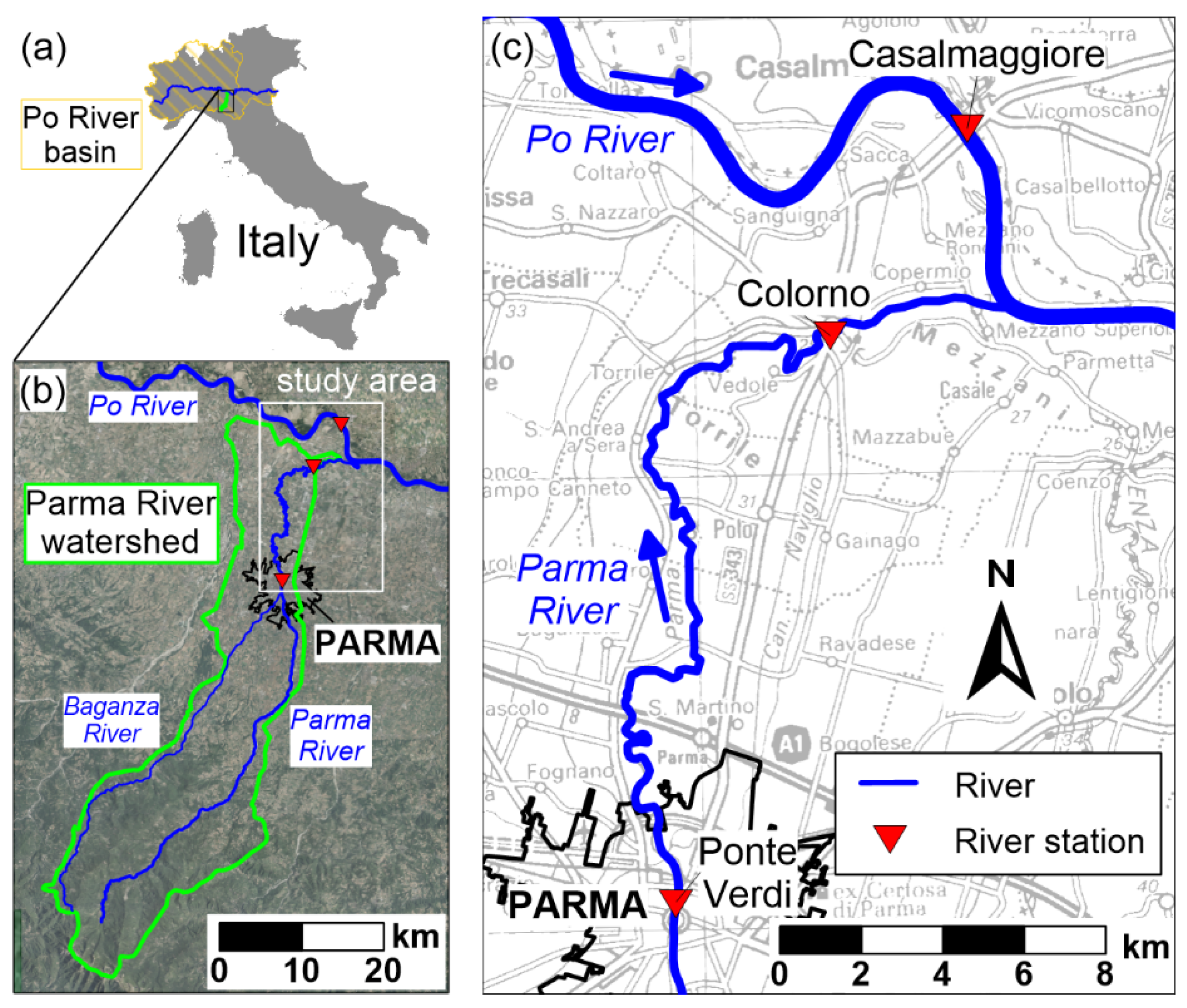
The Parma River (Italy, see Figure 1a) is roughly 92 km long from the headwaters to the confluence with the Po River (Figure 1b), but, in this work, we focused only on the lower stretch (32 km long) between the gauge stations of Ponte Verdi and Colorno (Figure 1c), which is fully bounded by artificial embankments that protect the surrounding lowlands. The most critical section of the river is inside the urban area of Colorno, where the condition of almost-zero freeboard was observed in the past during severe flood events, and where overtopping was experienced in 2017 with the subsequent flooding of a portion of the town. However, critical spots are very limited and well known by hydraulic authorities; hence, local overflows can be reduced or avoided by placing sandbags and flood barriers, provided that flood warnings are issued with adequate notice. Therefore, a reliable flood stage forecasting system can be particularly useful for supporting decision-makers about if/when to organize these emergency operations and to alert the population. For this specific case study, a few hours (6–9 h) can be considered sufficient to protect the vulnerable spots of the levee, also thanks to the activation of the town’s well-structured civil protection plan in case the weather forecasts indicate the possibility of an upcoming flood event.
In this study, we tested the performance of machine-learning methods in forecasting the flood stages in Colorno up to 9 h ahead, by exploiting the stage observations at the upstream station of Ponte Verdi. In fact, the catchment area between the two stations is negligible compared to the upstream basin, closed at the section of Ponte Verdi (approximately 600 km2); hence, the flood waves simply propagate without significant additional contributions along the river.
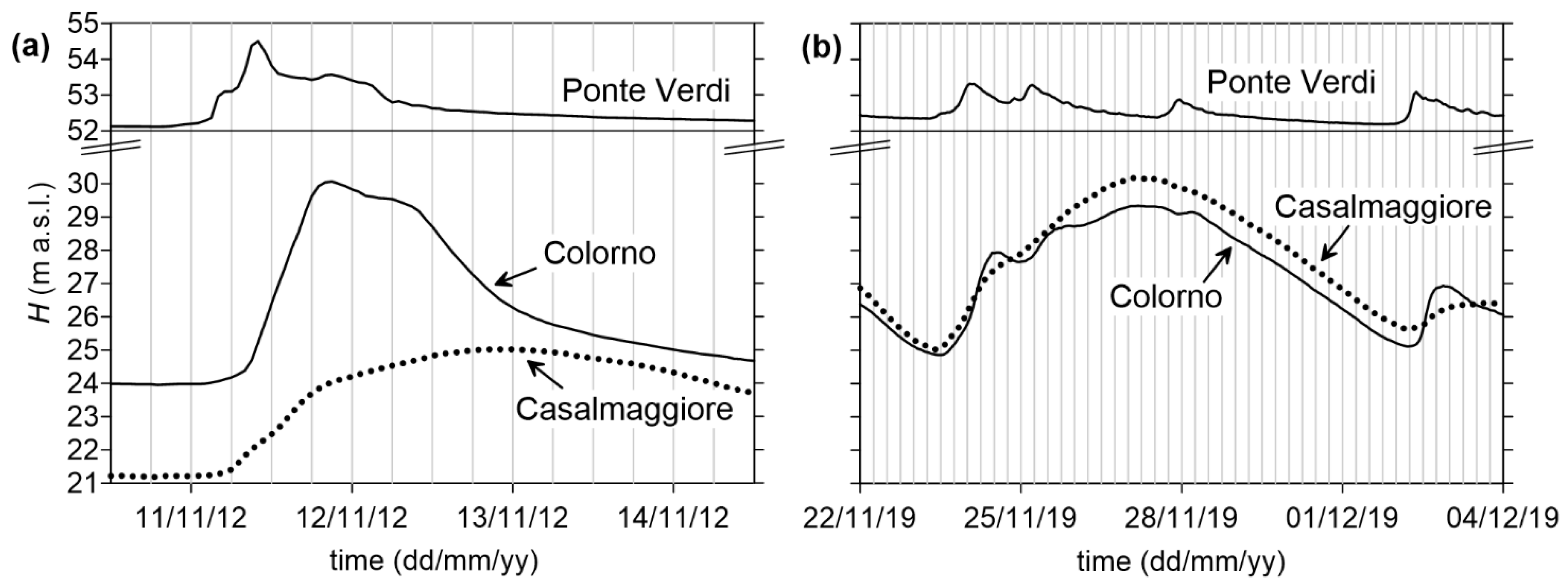
On the other hand, the water levels in Colorno can also increase due to backwater during flood events on the Po River, whose confluence is only 7 km downstream. For this reason, stage observations at the nearby station of Casalmaggiore (located on the Po River, roughly 5 km upstream of the confluence, see Figure 1c) are also considered when setting up the forecast model, as also suggested by Sung et al. [38] for tributaries. Indeed, the Po River is much larger than the Parma River: its catchment area, closed at the section of Casalmaggiore, is around 54,000 km2 (the full basin is 71,000 km2, see Figure 1a). While its low/moderate flows do not generate any backwater along the tributaries, its flood events, characterized by long durations and large water level excursions, often affect the downstream stretch of the tributaries for a few kilometers, also thanks to the low terrain slopes. As a qualitative example, Figure 2 reports the level time series at the three gauging stations for two flood events: the first is a flood event on the Parma River, while the second one is on the Po River. In the latter example, the high correlation of flood stages on the Po River (Casalmaggiore) and in Colorno is evident (a full correlation analysis including many flood events is presented in Section 3.3.1). The longer duration (and more gradual level variation) of Po River floods makes these events less critical for issuing alerts in Colorno, as the available modelling chain of the Po River basin can provide timely predictions of upcoming levels along this watercourse. However, even if this work aimed mainly at forecasting levels for the more “sudden” and short-lasting Parma River floods, considering stage observations in Casalmaggiore and Po River floods in the analysis is important to include the possibility of “combined” events.
Finally, we need to point out that rainfall data from the upstream catchment area of the Parma River cannot be easily used for real-time predictions in this case study. In fact, the presence of a flood control reservoir (a few kilometers upstream of the city of Parma), which is regulated on-line during flood events, can modify the response to rainfall in the downstream stretch of the river. Unfortunately, historical recordings of the gate regulations are currently not available; hence, we could not build a reliable forecast model based on all the relevant watershed data.
3. Materials and Methods
3.1. Machine Learning (ML) Models
3.1.1. Support Vector Regression (SVR)
SVR is an extension of the SVM method, based on the principle of structural risk minimization and originally developed for classification problems, to the case of regression problems. Here, the algorithm is very briefly recalled, while more details can be found, for example, in [41,42].
The key idea is to find a regression function f(x) that can approximate the target output y with an error tolerance ε. For nonlinear problems, the input vector x is previously mapped into a feature space by means of a nonlinear function ϕ(x), so the regression function becomes:
where w is the vector of weights, and b is a bias. The Vapnik’s ε-insensitive loss function is used to determine the penalized losses Lε as follows:
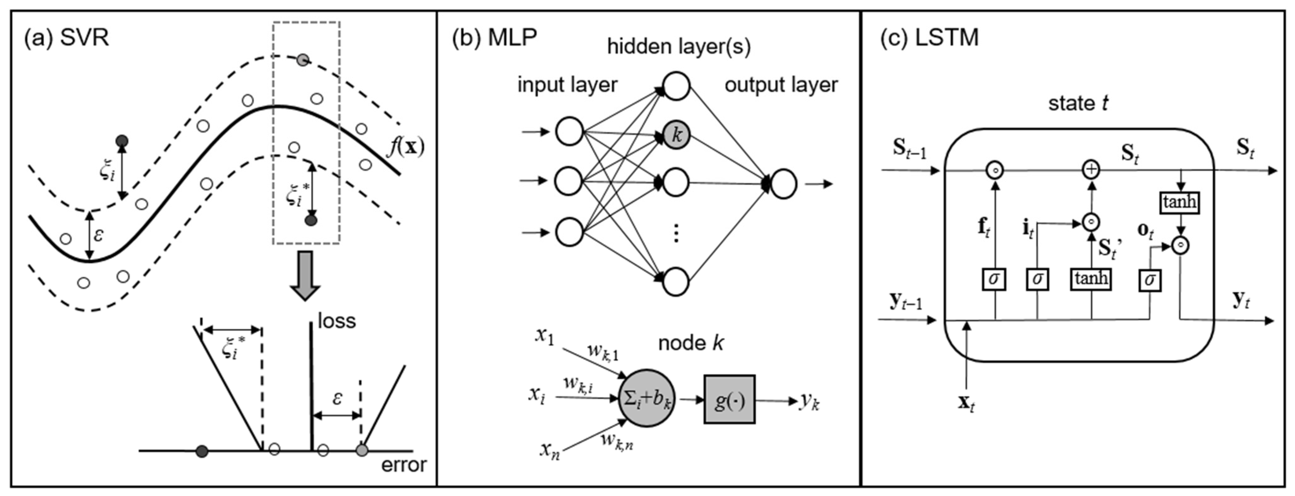
which indicates that only deviations larger than ε (i.e., values lying outside the ε-tube in Figure 3a) are unacceptable. The optimization problem aims to reduce these deviations while keeping the function as flat as possible, and it can be formulated as follows:
where ξi and ξi* are slack variables that express the upper and lower errors above the tolerance (Figure 3a), respectively, which are penalized via the positive constant C. The optimization problem in Equation (3) is then solved by introducing a dual set of Lagrangian multipliers αi and αi*, and it can be re-formulated as:
where is a kernel function that avoids the necessity of computing dot products in the feature space. Finally, the regression function can be rewritten as:
The main parameters for SVR are the error tolerance ε, which influences the generalization ability of the model, and the regulation constant C, which controls the smoothness of the regression function. Moreover, the kernel function may include additional parameters. For example, the radial basis function is frequently used as the kernel, and it requires the definition of the parameter γ (γ > 0):
3.1.2. MultiLayer Perceptron (MLP)
ANNs [41] are ML tools that were inspired by the ability of the human brain to learn from experience thanks to the biological neurons, which are connected and activated based on the input signals. In ANNs, neurons are actually computational units that receive input data, process them, and deliver an output signal. Among the ANN architectures, one of the most widely used is MLP, where neurons are arranged in three types of layers: one input and one output layer, and one or more hidden layers in between (see Figure 3b). These layers are usually fully connected, i.e., each neuron is linked to all neurons in the adjacent layers. The input layer has a number of nodes equal to the number of input features, which are read and passed on to the hidden layer, where the actual computations take place; finally, the output nodes deliver the final outcome. This type of network, characterized by a one-directional flow of data, is called a “feed-forward” network. Overall, the MLP model can be represented in compact form as a function that maps an input vector x into an output y (which may be either a single value or a vector):
This expression actually encompasses the computations performed in several nodes. In fact, each neuron k in the hidden layers (see inset in Figure 3b) performs a weighted sum (with weights wk,1,…, wk,n) of the n inputs from the previous layer (x1,…, xn), plus a bias bk, and gives an output yk through an activation function g:
The activation function is introduced to capture nonlinearity. If the MLP architecture is fixed, the optimization process (known as “training”) of the network consists of adjusting the weights and biases of all neurons in order to minimize the loss function between the output of the model in Equation (7) and the target output. The training of ANNs is commonly performed using the back-propagation algorithm (for more details, see [41]).
The most important parameters of the MLP model are its architecture (i.e., the number of neurons and hidden layers), and the activation function g. Commonly used activation functions are the sigmoid or logistic function (σ), the hyperbolic tangent function (tanh), and the Rectified Linear Unit (ReLU) function:
3.1.3. Long Short-Term Memory (LSTM)
The class of neural networks that include loops in the inter-neural connections are called Recurrent Neural Networks (RNN), as opposed to feed-forward networks. RNNs were introduced to allow learning temporal sequences, even if long-term dependencies could not be handled due to the vanishing gradient problem. To overcome this drawback, Hochreiter and Schmidhuber [43] presented a special type of RNNs, called LSTM.
In between the input and output layers, LSTM networks are composed of one or more memory cells (Figure 3c) with structures called “gates,” namely the input (i), forget (f), and output (o) gates, whose function is to control the cell state. The forget and input gates control the information to be removed or added to the cell state, while the output gate determines the output in a selective way. At each time step t, the gates are fed with both the input xt and the output yt−1 from the memory cell at the previous time step t − 1. The following operations are performed:
where ft, it, and ot, are the states of forget, input, and output gates at time t, respectively; St and St−1 are the cell states at times t and t − 1, respectively; σ and tanh are the activation functions in Equations (9) and (10), respectively; Wf, Wi, Wo, WS, and bf, bi, bo, bS, are the weights and biases of the forget, input, and output gates and candidate state variable St′, respectively; finally, the symbol ◦ indicates the element-wise multiplication. Similar to other neural networks, once its architecture (number of unit cells) is defined, the LSTM network is trained to adjust the weights and biases by means of algorithms trying to minimize the loss function between target output and model output, which can be expressed in compact form as:
3.1.4. Metrics for Model Evaluation
The evaluation of the forecasting abilities of the ML models in this study is based on the root-mean-square error (RMSE), the mean absolute error (MAE), the coefficient of correlation (CC), and the Nash–Sutcliffe efficiency coefficient (NSE). These goodness-of-fit metrics are defined as follows:
where N is the number of samples in the dataset, and yi,obs and yi,pred are the observed and predicted stages, respectively, while and are the mean values of observations and predictions, respectively. RMSE and MAE have the same units as the original variables (meters in this case), while CC and NSE are non-dimensional measures. A perfect match between observations and predictions is characterized by RMSE and MAE equal to 0, and CC and NSE equal to 1. For the evaluation of the models based on these metrics, we refer to the criteria suggested by [44], where a performance rating of “very good” is assigned to models providing NSE ≥ 0.9 and RMSE ≤ 0.31∙SD, where SD is the standard deviation of observations; when NSE ≥ 0.8 and RMSE ≤ 0.45∙SD, the model is classified as “good,” while values of NSE ≥ 0.65 and RMSE ≤ 0.83∙SD identify an “acceptable” performance; otherwise, the model rating is “unsatisfactory.”
Additionally, the models’ performance in forecasting the peak level for each flood event was considered. To this aim, the predicted peak of each event was extracted from the dataset, and the errors were quantified using the RMSE, the NSE, and the mean absolute percentage error (MAPE):
where Nev is the number of events, and the percentage error is relative to the peak water depth di,obs.
3.2. Availability of Data
The recorded water stages at the stations of Colorno, Ponte Verdi, and Casalmaggiore are available from 2012 to 2020, at time intervals of 10 min. The original data were down-sampled to hourly values.
Data for 47 flood events were extracted from this time series. Actually, among these, only 25 events were characterized by a peak level exceeding the first “alert threshold” at Colorno (i.e., 27.7 m a.s.l.), but smaller floods (with peaks up to 1 m below this alert level) were additionally included in order to enlarge the dataset. All events were categorized in four groups (see Table 1): large, medium, and small floods on the Parma River, and Po River floods causing backwater in Colorno. Large floods were identified as those with a peak level that exceeds the highest alert threshold (i.e., 30.7 m a.s.l.). All events with backwater from the Po River were included in the same group, regardless of the peak level. Please notice that the values of the above-mentioned alert thresholds are those officially defined by the hydraulic authorities. The complete list of events is reported in Table S1 in Supplementary Materials.
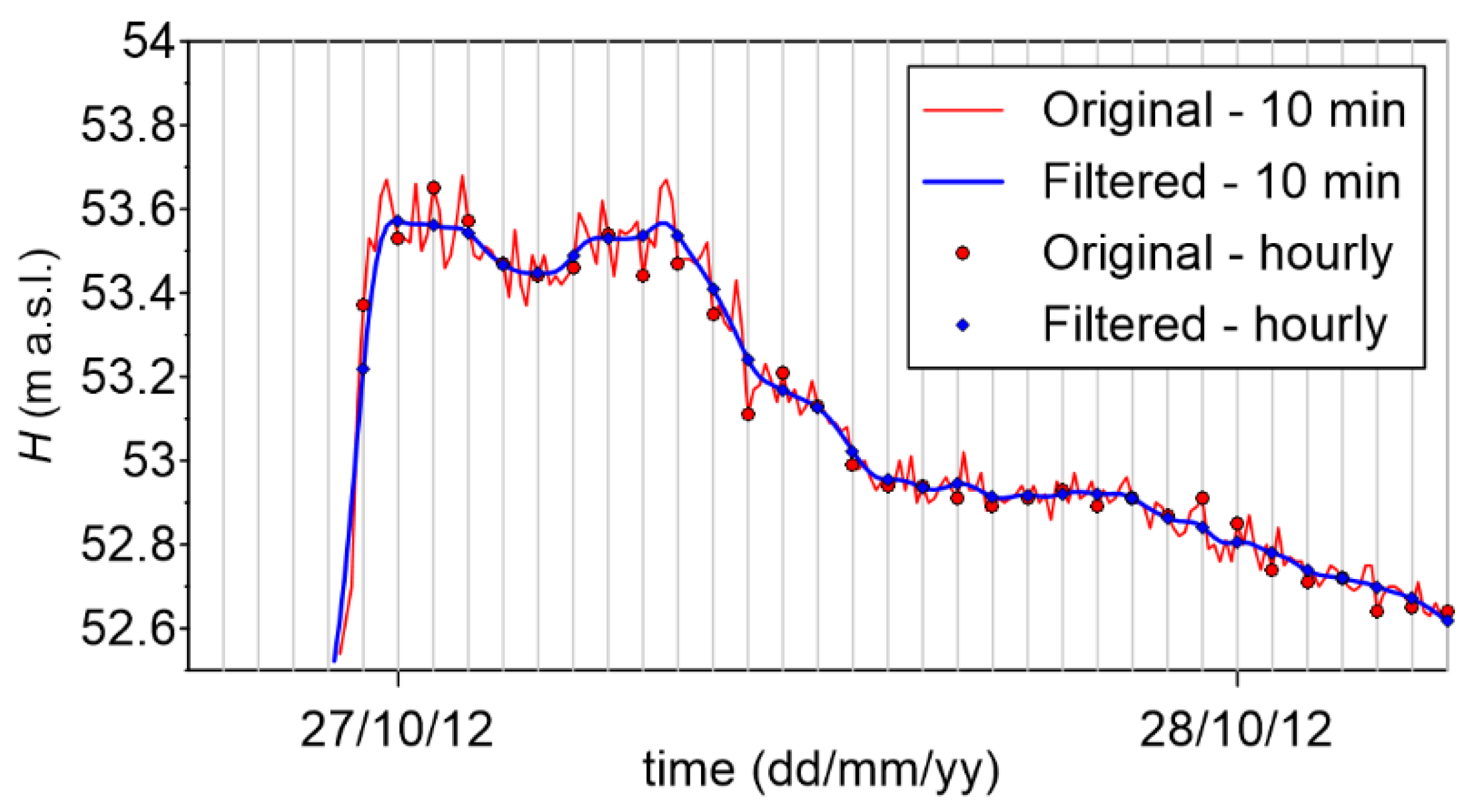
The original recorded water levels at Ponte Verdi station were characterized by small unphysical oscillations (5–10 cm), attributable to the instrumentation. Despite the down-sampling to hourly data, preliminary tests showed that these fluctuations may influence the predictions of ML models, especially for the longer lags (6–9 h ahead). Therefore, the original water level time series at Ponte Verdi (at 10 min intervals) was filtered and only later down-sampled to hourly values. An example of original and processed data is shown in Figure 4. We used a smoothed particle hydrodynamics [45] interpolation of the original data:
where is the filtered water stage at the i-th time step, Δt is the original time interval (10 min), n is the number of time steps in the smoothing window (I − L, I + L) (with L = 40 min in this case), and ωij is the cubic spline kernel [46].
3.3. Model Setup
All ML models were built in Python 3.8 using Tensorflow (version 2.2) and scikit-learn (version 0.23) libraries. In the following, the main steps for setting up the models are detailed.
3.3.1. Input Selection
The aim of each ML model was to forecast the water stage in Colorno at time t + X (where X varies between 1 and 9 h). Input variables for the ML model included the stage observations at Ponte Verdi and Casalmaggiore at times t − T,…, t (where T is the size of the past time window of relevant observations), but the stage observations at Colorno at previous time steps were also considered, given their high correlation with the output value.
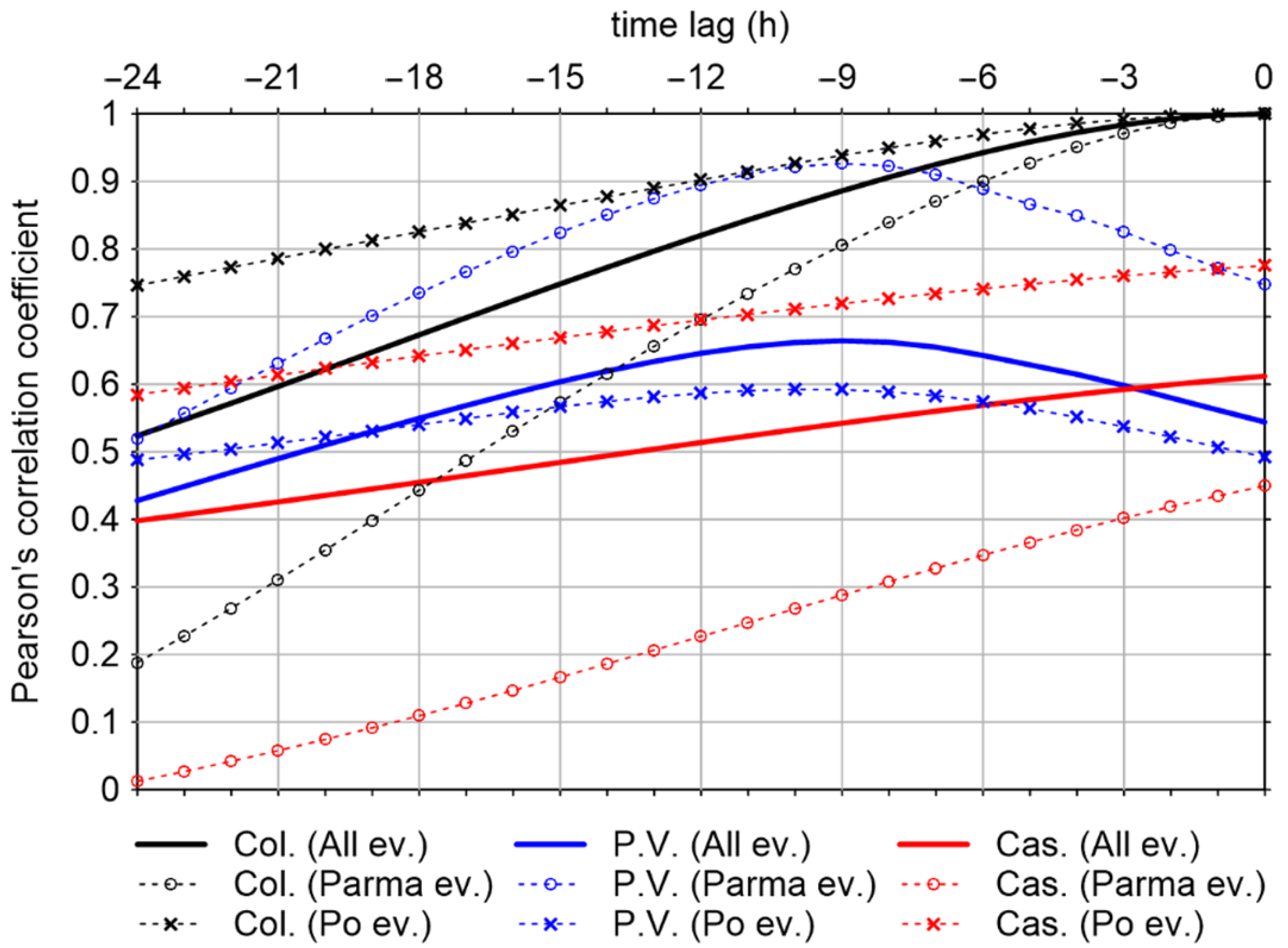
A correlation analysis was performed in order to identify the correct size of the past time window (i.e., T). We indicate the water stages with H, and the subscripts “P.V.”, “Cas.”, and “Col.” are used to identify the river stations of Ponte Verdi, Casalmaggiore, and Colorno, respectively. The coefficient of correlation between the values HCol.(t) and each candidate input variable (HP.V.(t − i), HCas.(t − i), and HCol.(t − i), with i = 1,…, 24) was calculated. Results are reported in Figure 5. If we consider data from all events (thick lines), the correlation with the stage in Ponte Verdi has a maximum (CC = 0.66) at −9 h, which is approximately the flood travel time between the two stations along the river. However, if we limit the analysis only to flood events on the Parma River, the correlation is much higher (maximum CC = 0.93, still at −9 h), and the CC remains larger than 0.9 up to −12 h; in this case, the stage in Casalmaggiore does not show a significant correlation with the stage in Colorno (CC < 0.5). Conversely, if we only analyze data from the Po River flood events, the CC related to the stage in Casalmaggiore is in the range 0.7–0.8 between −12 and −1 h, showing a larger correlation. Finally, past observations in Colorno have a significant correlation with the current stage (CC > 0.8 up to −12 h if we consider all events), which confirms that these data should be included among the input variables. Overall, as the objective was to set-up a model able to predict stages in Colorno for all types of events (Parma and Po River floods, and possibly “combined” events), a time lag of 12 h was selected for data from all stations. In addition, the correlation analysis supports the choice of the maximum time lag for future predictions as Xmax = 9 h.
In summary, the output of the ML model was only one, i.e., HCol.(t + X), while the following 36 input variables were used:
- HP.V.(t − 11),…, HP.V.(t − 1), HP.V.(t);
- HCas.(t − 11),…, HCas.(t − 1), HCas.(t);
- HCol.(t − 11),…, HCol.(t − 1), HCol.(t).
As we are interested in multiple predictions (X = 1,…, 9 h), 9 models were defined for each ML method. It is worth mentioning that, while SVR only allows one output, both ANN and LSTM can provide multiple outputs, and only one model could have been set-up to provide the full prediction (with outputs HCol.(t + 1),…, HCol.(t + 9)). However, we decided to set-up separate models for each time lag to ensure a fair comparison between the three ML approaches herein adopted. In fact, Campolo et al. [19] showed that predictions at the same time lag using single- or multiple-output models are different, as the loss function to be minimized during training is not the same.
3.3.2. Training Process
Overall, 9484 hourly data are available for X = 1 h, while for the longer time lags, this value slightly decreases due to few missing values at the end of each event (e.g., 9108 data for X = 9 h).
In order to align stage observations (expressed in m a.s.l.) from different stations, all data were normalized to the interval (0, 1), where the minimum and maximum values were selected according to the gauged river cross-sections. In particular, for each station, the minimum allowable value was set equal to the bed elevation, while the maximum was set equal to the local levee crown elevation, incremented by 50 cm to consider possible overtopping. Regarding Colorno station, the highest recorded level (during a severe flood that occurred in 2017) corresponds to the normalized value of 0.95. After training the model and making predictions, forecasted data were scaled back to their original units to perform comparisons with the observed values and compute error metrics.
Data from the 47 flood events considered in this work were divided into sets for training (32 events), validation (7 events), and testing (8 events). The splitting was performed randomly, but we ensured that the mean and standard deviation of data from different sets were comparable, and that different types of events were represented in each dataset, according to the partition reported in Table 2. The percentage of data included in each dataset slightly depends on the duration of the events (selected randomly), but, on average, 65% of data belong to the training set, 16% to the validation set, and 19% to the testing set. The training set was used to fit the models’ internal parameters (weights, biases, etc.), while the validation set was used here to tune the models’ hyperparameters and prevent overfitting. Finally, the testing set was used to evaluate the models’ performance on unseen data.
Usual strategies reported in the literature were adopted to avoid overfitting. The SVR model was trained using 5-fold cross-validation to prevent overfitting, while, for the MLP and LSTM models, overfitting was avoided by implementing an early stopping procedure, which interrupts the training when the loss function for the validation dataset no longer improves or starts to increase. These latter models were trained using the efficient Adam optimizer and selecting the mean squared error as the loss function.
Moreover, both the MLP and LSTM are known to provide unreproducible results, due the random initialization of weights. Berkhahn et al. [28] tested an ensemble approach to capture this uncertainty, i.e., the training of the MLP model was repeated Nens times, and the mean prediction of the Nens realizations for each data sample was used as final prediction. In this work, the same approach was adopted for both the MLP and LSTM models, with Nens = 10.
3.3.3. Model Structure Definition
For all models, some important hyperparameters need to be optimized. Three random train/validation/test splits were considered in order to select the “best” configuration for each model as that providing the lowest RMSE on average. In order to reduce the computational burden, only the models with lag times equal to 3, 6, and 9 h were optimized. However, for all models, we observed that the best set of hyperparameters was almost insensitive to the time lag, so the same set was finally adopted for all time lags.
The SVR model requires the optimization of hyperparameters C and ε (see Section 3.1.1), and the additional parameter γ for the kernel function used for this application, i.e., the radial basis function (Equation (6)), which is widely used for regression problems [32]. The best hyperparameters were determined using a grid-search procedure, which ultimately provided the following set: C = 20, ε = 0.005, and γ = 0.1.
The MPL model requires the definition of the best architecture for the network (number of hidden layers and neurons). The Rectified Linear Unit (ReLU) activation function was adopted in this work. A trial-and-error optimization was performed, by increasing the network complexity until additional neurons and layers did not further improve the results. The best configuration is characterized by only one hidden layer with 16 neurons.
Similarly, the LSTM model requires the definition of the number of units. By trial-and-error, we selected the configuration with 10 units: increasing the number of units did not improve the results significantly.
4. Results and Discussion
4.1. Comparison of Models’ Performance
Table 3 summarizes the performance metrics (RMSE, MAE, CC, and NSE) of the different ML models for three time lags, namely 3, 6, and 9 h ahead. Depending on the random splitting of flood events into training, validation, and testing sets, the metrics chosen to evaluate the models’ performance can have slightly variable values. For this reason, the comparison here was based on the average measures obtained from 20 different splits (see Table S2 in Supplementary Materials).
The training and validation results were slightly better than those concerning the testing dataset, as expected. In general, the predictive performance of all models (testing dataset) was quite good, as we obtained a 3 h-ahead forecast with an RMSE of the order of 7–9 cm, which increased to 13–15 cm (25–26 cm) for the time lag of 6 h (9 h). For the purpose of forecasting, these errors are totally acceptable. In this case study, the SD of water level observations in Colorno was equal to 1.37 m (full dataset); hence, the RMSE and MAE were in the range 0.05–0.19 and 0.03–0.11 times the SD, respectively: these results indicate an overall “very good” performance for all models and time lags, based on the classification reported by [44]. Moreover, the CC and NSE were very close to 1: the NSE was higher than 0.98 for all models and time lags (NSE > 0.99 for 3–6 h), while the CC was below that threshold only for the longest time lag (still, it remained higher than 0.96). This confirms the “very good” model performance according to [44], as NSE ≥ 0.9. Incidentally, the study of Leahy et al. [39], who also exploited water level observations for flood forecasting with an ANN model, reported CC and NSE values around 0.98–0.99 for a 5 h-ahead prediction, which is in line with our findings for the 3–6 h forecasts, despite some differences between the two case studies.
Even if all models ensure a good prediction accuracy, when the performances of different models are compared, we can observe that SVR and LSTM provided lower errors (in terms of both RMSE and MAE) compared to MLP, which performed consistently worse for all time lags, although the differences were less significant for the time lag of 9 h. Overall, the best performance was provided by the SVR model, which was characterized by a slightly lower RMSE than the LSTM model; moreover, the MAE was always lower, even when the RMSE, CC, and NSE values were very close (e.g., time lag of 9 h).
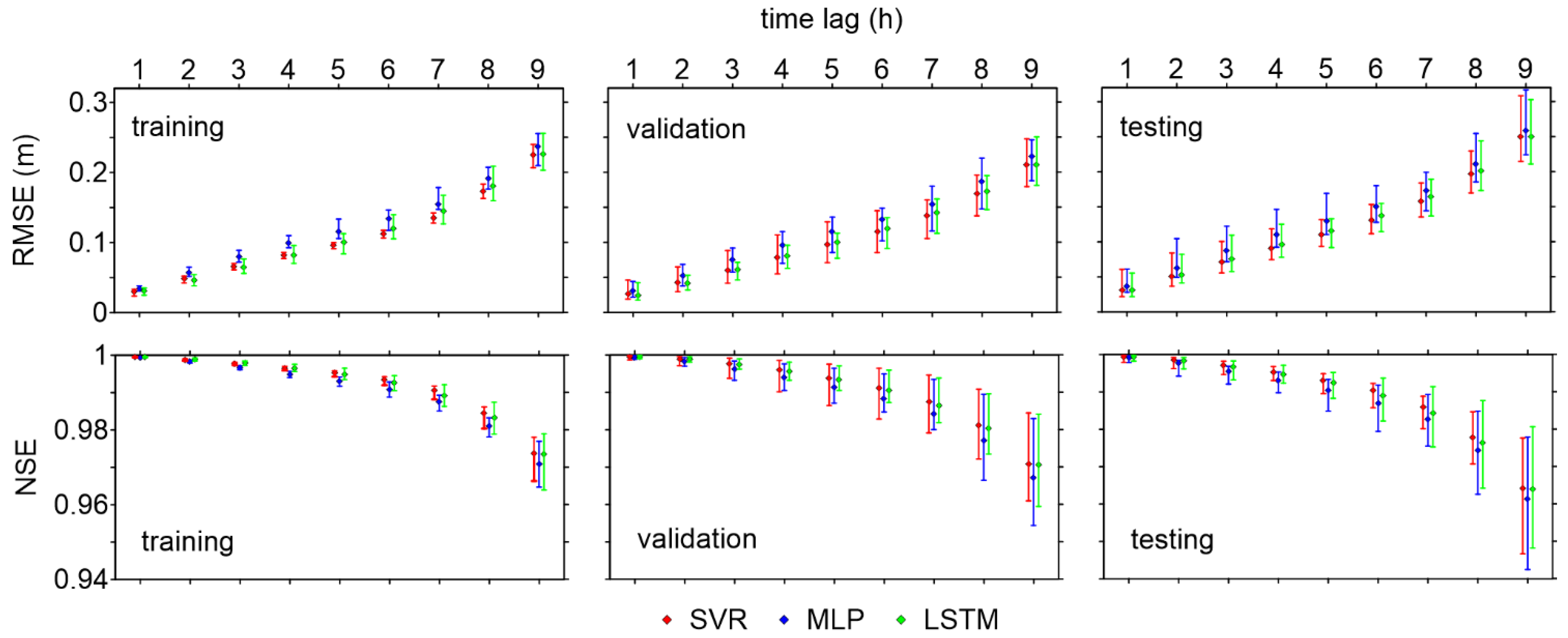
As anticipated from Table 3, the adherence of predictions to observations decreased with the time lag. This finding was expected, as it was observed in a number of previous studies about flood forecasting [19,32]. Figure 6 shows the trend of two goodness-of-fit measures (RMSE and NSE) as the forecast horizon grows. Similar trends could be observed for MAE and CC (not shown here, for brevity). The RMSE was of the order of 3 cm for the 1 h-ahead prediction and grew almost linearly up to 7 h ahead (15–17 cm for the testing dataset): for longer time lags, the error seemed to grow more quickly with the forecast horizon. The NSE also dropped below 0.98 for the 8 and 9 h-ahead predictions. Overall, the SVR and LSTM models performed comparably for all time lags, while the MLP consistently provided slightly worse metrics. Moreover, the vertical bars in Figure 6 indicate the range of variability of the error metrics for the 20 different train/validation/test splits. Compared to the training dataset, the variabilities of RMSE and NSE for the validation and testing datasets were more pronounced, as (i) the ML models are fit based on the training dataset, and (ii) the larger size of the training dataset can “mask” a few inaccurate predictions. The range of variability was larger for the longest time lags. Indeed, it remained roughly below 5 cm up to 7 h ahead for all models regarding the testing dataset, and then increased up to 9 cm for the 9 h-ahead prediction—in this case, the RMSE could be larger than 30 cm.
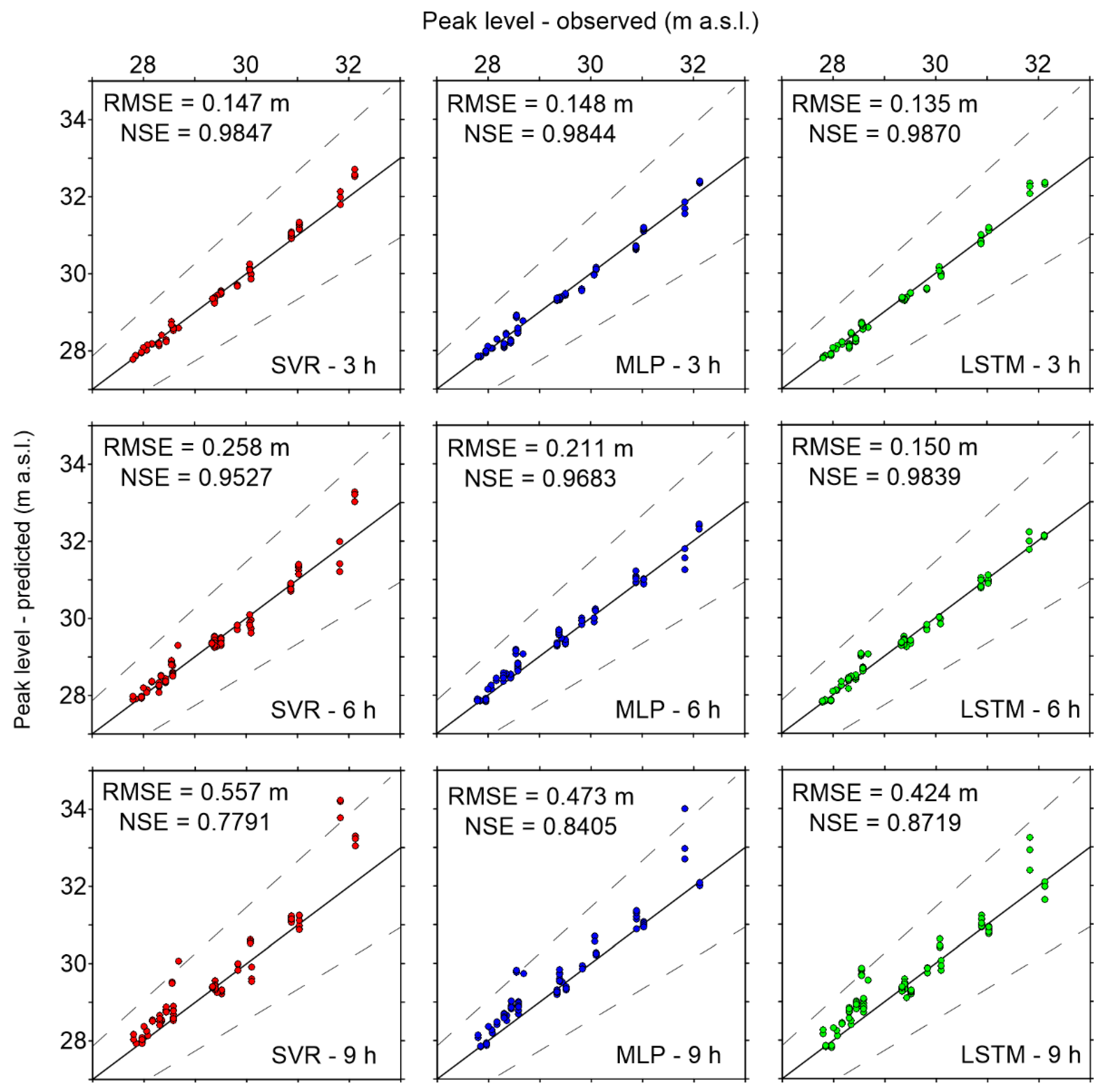
The errors on the peak levels are also of great interest to evaluate the flood forecasting performance of the ML models. We limited the analysis to flood events with an observed peak level higher than the first alert threshold. The SD of these peak values was equal to 1.25 m. Table 4 reports the RMSE, NSE, and MAPE of predicted peaks (obtained from 20 random train/validation/test datasets) for three time lags (3, 6, and 9 h). As expected, these results confirm that the errors evaluated for the training dataset were lower than those for validation and testing also for the peak levels, and that the errors grew with the forecast horizon. Focusing on peak levels obtained from the testing datasets, the best performing model was undoubtedly LSTM, which provided a lower RMSE and a higher NSE for all time lags, compared to the other models. SVR and MLP had a similar performance for the 3 h-ahead prediction, while for the longer time lags, the SVR model provided a higher NSE and lower RMSE (though the MAPE of the MLP model remained slightly larger than that of SVR). More in detail, Figure 7 shows the scatter diagrams of the observed and predicted peak levels for SVR, MLP, and LSTM for the same three time lags, limited to the testing sets (for training and validation, similar plots are reported in Figures S1 and S2 in Supplementary Materials). These plots confirm that SVR was the worst performing model, especially for the longer forecast horizons, where the largest peaks were systematically overestimated, with errors higher than 20% of the observed peak water depth for 9 h-ahead predictions. The MLP predictions were closer to the observations than those of SVR for the time lags of 6 and 9 h. On the other hand, LSTM forecasted the peak levels with errors below 50 cm for the time lags of 3 and 6 h (with RMSEs of the order of 13–15 cm, and NSE > 0.98). Similar to the other ML models, however, its predictions became less accurate for the forecast horizon of 9 h. According to the model evaluation criteria [44], all models provided a “very good” performance for the time lags of 3 and 6 h, while only MLP and LSTM could still be classified as “good” models (NSE > 0.8, and RMSE < 0.45∙SD) for the time lag of 9 h. Actually, all models seemed to predict the peak levels 9 h ahead quite inaccurately, with RMSEs of the order of 40–50 cm, which may be too large an error for a reliable forecast. Besides, a common tendency to overestimation of the peaks around 28–29 m a.s.l. could be identified. Most of these peaks correspond to Po River flood events (this behavior is briefly discussed in the next section).
4.2. Predictive Validity
In this section, some examples of forecasts of flood levels are reported. In this case, we focus on the results obtained from two selected train/validation/test splits. Full details on the data splitting and on the performance metrics for these two examples are reported in Tables S3 and S4 in Supplementary Materials.
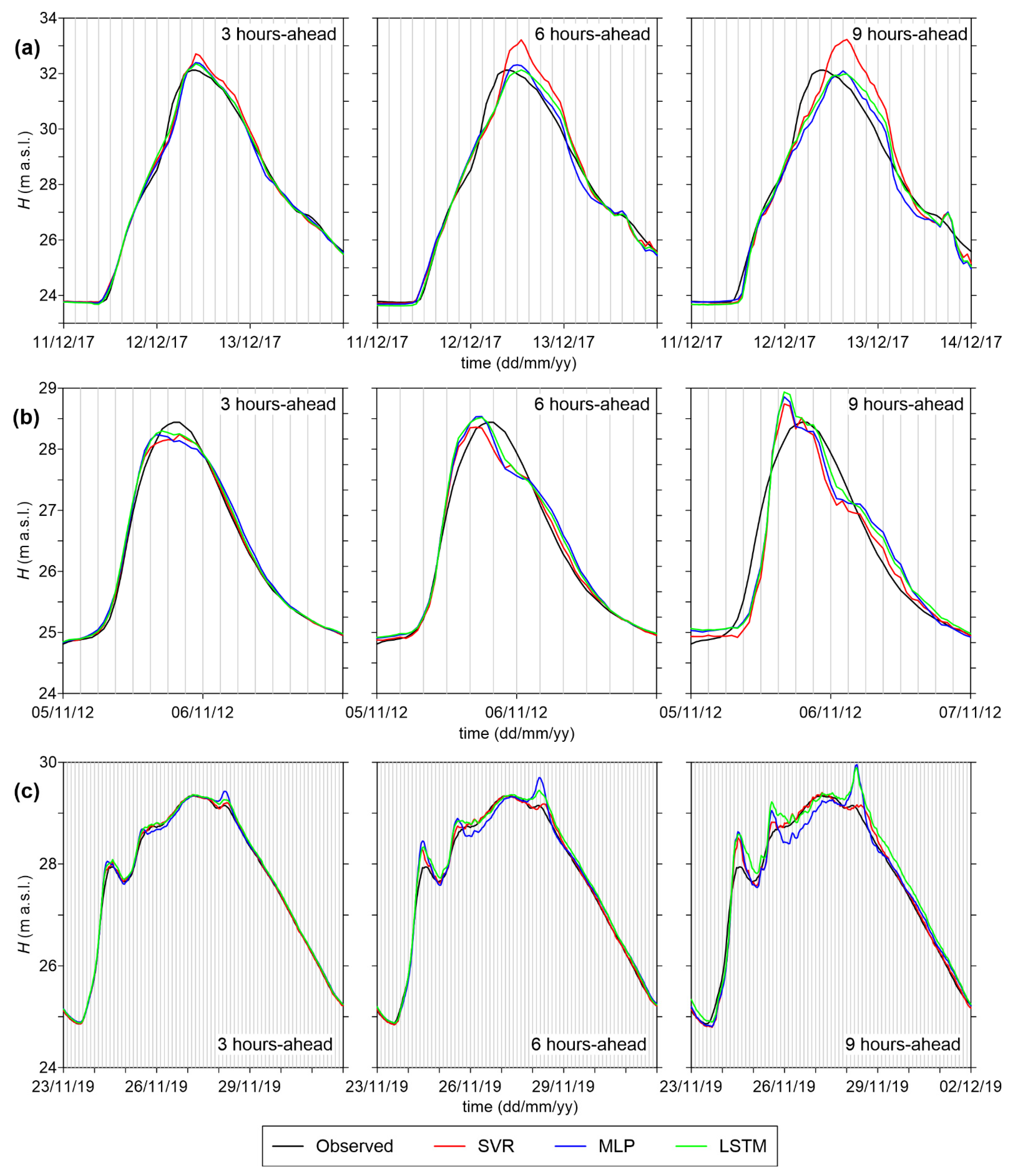
The first example is taken from a split characterized by error metrics (Table S3) below the average values previously reported in Table 3 for all ML models. The testing dataset includes the flood event that occurred in March 2015, which is characterized by the third largest peak ever recorded in Colorno (31.03 m a.s.l.), while the influence of the Po River levels is negligible. Figure 8a compares the forecasted levels 3, 6, and 9 h ahead with the observed values for this event. In these plots, the series of levels obtained from SVR, MLP, and LSTM models simply consist of the sequence of single predictions at different times. All models provided excellent level forecasts for the time lag of 3 h; moreover, the 6 h-ahead prediction was still very good for MLP and LSTM, while SVR overestimated the peak (roughly 30 cm); finally, the 9 h-ahead forecasts were less accurate for all models, though still acceptable. Overall, SVR seemed to predict the beginning of the falling limb of the flood event with a few hours’ delay for the longer time lags.
In Figure 8b,c, two additional events from the testing set of this split are shown. Figure 8b refers to the October 2012 flood event (“medium” Parma River flood): all ML models provided similar level forecasts, with a slight tendency to underestimate the peak for the shorter time lag (3 h), and to overestimate it for the longer time lag (9 h). Figure 8c shows observed and predicted levels for the flood event of February 2014 on the Po River; while, overall, the 3 h-ahead forecasts were good for all models, peak overestimations can be observed for the longer time lags (with MLP performing the worst for this event). This inaccuracy was due to the high correlation of levels in Colorno with the simultaneous levels in Casalmaggiore for Po River floods (see Section 3.3.1): the stage in Colorno increased almost “in phase” with the levels downstream during this type of flood; hence, forecasts with long time lags are not expected to be very accurate for these events. Conversely, for Parma River floods, the relatively long travel time of the flood wave from Ponte Verdi to Colorno (roughly 9 h) ensures that ML models are capable of providing acceptably accurate forecasts up to a few hours ahead for these events.
We also analyzed the ML models’ forecast for a split where the event with the largest peak ever recorded in Colorno was included in the testing set, with the aim of verifying the ability of the models to predict flood levels exceeding the largest values seen during training. For this split, the overall error metrics (Table S4) were close to the average values of Table 3 for MLP and LSTM, and slightly higher for SVR. Observations and forecasts for the most severe flood event of Colorno (occurred in December 2017 and characterized by a peak level equal to 32.12 m a.s.l.) are compared in Figure 9a. While all models were capable of predicting the flood stages well with a time lag of 3 h, for the longer time lags, the peak was reached with some delay (about 3 h for 6 h-ahead forecasts, and 6 h for 9 h-ahead ones), and SVR largely overestimated the peak levels. Forecasted levels for two additional events from this testing set were also plotted, namely the events of November 2012 (Figure 9b) and November 2019 (Figure 9c). The first one is a “medium” Parma River flood, and ML models performed similarly to the case of the previous split (Figure 8b), even if the peak overestimation for the 9 h-ahead prediction was more pronounced. The second event is a Po River flood: in this case, the forecasted levels were quite good even for the longer time lags, probably thanks to the very slow and gradual level variation. The SVR model performed particularly well in predicting flood stages for this event.
4.3. Example of Application
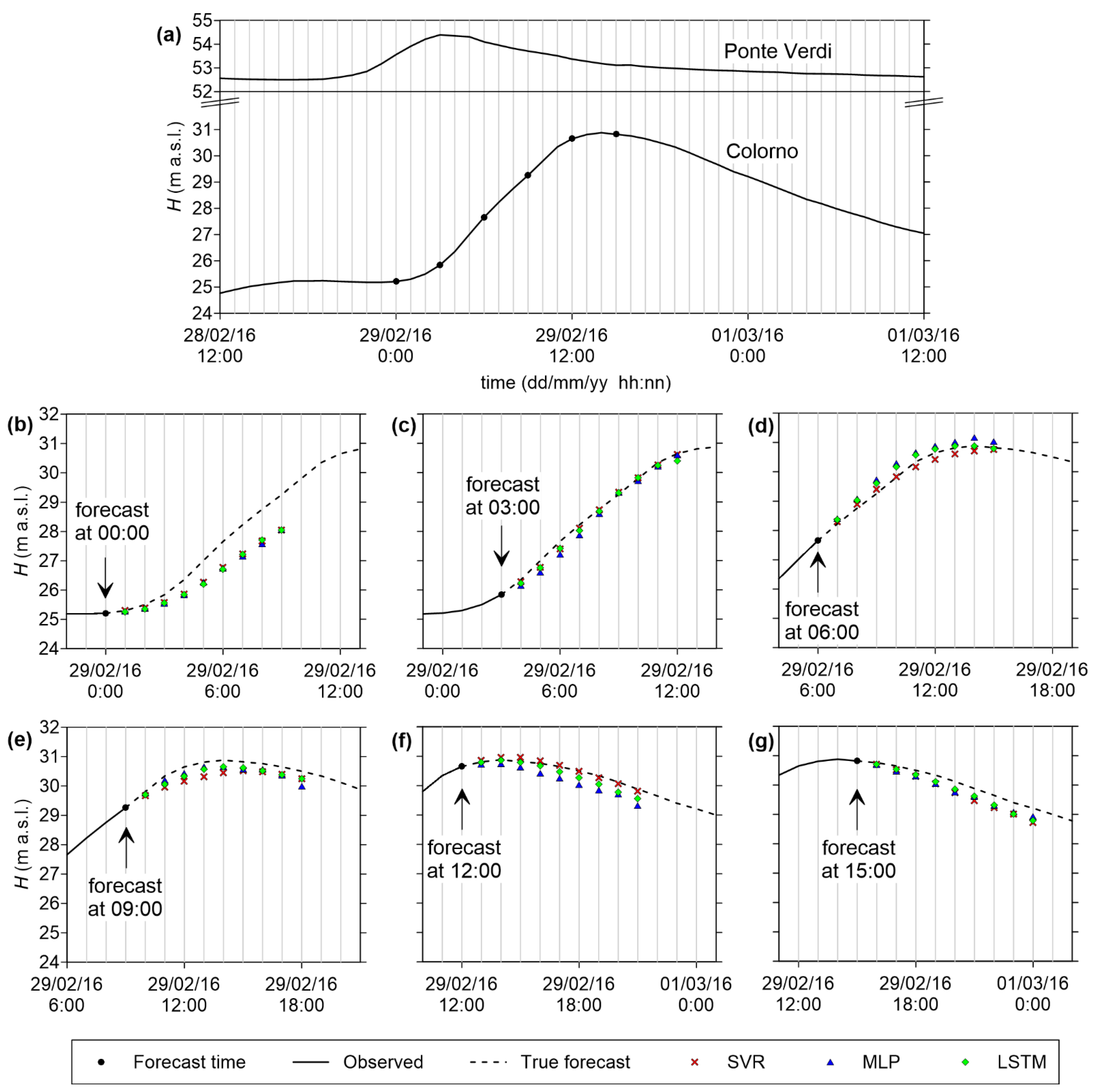
In this section, an example of an application of ML models for flood forecasting is presented. We selected the flood event of 28 February–1 March 2016, whose peak level (30.88 m a.s.l.) was the fourth largest peak ever recorded at Colorno station. For this event, the influence of levels downstream (Casalmaggiore) was not significant; hence, Figure 10a only reports the recorded levels at the river stations of Ponte Verdi and Colorno. The ML models’ forecasts (1 to 9 h ahead) are shown in Figure 10b–g at selected times.
In all phases of the flood, the trend of water levels in Colorno (rising, falling, peak) was correctly identified by all models. The early stages were underestimated (Figure 10b), probably due to the very gradual initial increase in levels at Ponte Verdi station. The rising limb was very well predicted for all time lags (Figure 10c), while the ML models provided slightly more variable results close to the peak, which, however, deviated from the actual observations less than 30 cm even for the 8–9 h-ahead prediction (Figure 10d,e). In the falling limb of the hydrograph (Figure 10f,g), there was a tendency to underestimate the water stages for the longer time lags. Overall, all ML models appeared suitable to provide real-time forecasts for this large flood event in Colorno.
4.4. Computational Times
The ML models were also compared regarding the computational time required for training (including pre- and post-processing data). An average value was obtained from multiple runs of training (>100), including different train/validation/test splits and different forecast horizons. Table 5 reports the average times for SVR, MLP, and LSTM. For the two latter models, both the computational times required for training a single model and for training an ensemble of 10 models were reported. The training time increased with the model’s complexity; hence, MLP took roughly three times more than SVR to be trained, and LSTM five times more than MLP. Obviously, the training time for an ensemble of 10 models (for MLP and LSTM) could be largely reduced by running computations on parallel cores.
However, the longer training times of MLP and LSTM may not be an issue for practical purposes, as the trained models can be saved and later used for forecasting. For this reason, Table 5 also reports the average time necessary for providing the full prediction (1 to 9 h ahead) with data pre- and post-processing. Again, MLP and LSTM required slightly longer prediction times than SVR did due to the choice of adopting an ensemble of 10 models. In any case, all models only took a few seconds (up to one minute) to deliver their forecasts, thus confirming the suitability of ML models for real-time applications.
5. Conclusions
In this work, we selected the case study of the Parma River (Italy) to evaluate the applicability of machine-learning algorithms to set-up a real-time flood forecasting model that is only based on observed water stages. This kind of “data-driven” approach has the advantage of avoiding the setup and calibration of physically based rainfall-runoff and/or flood routing models, and of being characterized by much lower execution times compared to these latter models. This work is particularly focused on the prediction of flood stages at a critical river station (Colorno) based on upstream stage observations (Ponte Verdi), though downstream stages (Casalmaggiore) were also included in order to consider possible level increases due to backwater from the Po River. The forecast horizon for this specific case study was limited to 9 h, which is the approximate flood travel time between Ponte Verdi and Colorno. Accurate stage predictions with a lead time of a few hours can be particularly useful for issuing flood warnings and taking timely actions to prevent local levee overtopping (e.g., placing sandbags and flood barriers at some well-known critical spots along the levee).
We compared three different ML models, namely SVR, MLP, and LSTM. Our results showed the following:
- In general, all models are able to provide sufficiently accurate stage forecasts up to 6 h ahead (RMSE < 15 cm, and NSE > 0.99), while prediction errors increase for longer lead times. The error on the peak levels also becomes very large for 9 h-ahead forecasts;
- SVR is characterized by the best RMSE values, and also by the shortest computational time. However, its accuracy on the peak levels is lower than those of the other models, especially for intermediate (6 h) and long (9 h) lead times;
- MLP presents the largest errors among the three models considered here, but the analysis of its predictive validity shows that it can still be considered suitable for practical purposes;
- LSTM performs similarly to SVR regarding the goodness-of-fit measures for the testing dataset, but it appears much more accurate in predicting the peak levels. Hence, despite the longer computational times required for the training phase, this ML model can be considered the best candidate for setting up a robust operational model for real-time flood forecasting.
Supplementary Materials
The following are available online at https://www.mdpi.com/article/10.3390/w13121612/s1. Table S1: List of flood events considered in this work (ordered by descending peak level for each type of event), Table S2: Random splitting of flood events into train/validation/test for each of the 20 runs (t = training; v = validation; x = testing), Table S3: Split #3 (example of Figure 8): comparison of ML models’ performance for training, validation, and testing dataset, Table S4: Split #20 (example of Figure 9): comparison of ML models’ performance for training, validation, and testing dataset, Figure S1: Comparison of observed and forecasted peak levels in Colorno (training dataset) for time lags of 3, 6, and 9 h, Figure S2: Comparison of observed and forecasted peak levels in Colorno (validation dataset) for time lags of 3, 6, and 9 h.
Author Contributions
Conceptualization, P.M. and R.V.; methodology, S.D., R.V. and P.M.; formal analysis, S.D.; data curation, S.D.; writing—original draft preparation, S.D.; writing—review and editing, S.D., R.V. and P.M.; supervision, P.M. and R.V. All authors have read and agreed to the published version of the manuscript.
Funding
This research received no external funding.
Institutional Review Board Statement
Not applicable.
Informed Consent Statement
Not applicable.
Data Availability Statement
The river stage data used in this work can be downloaded from the Dext3r portal (https://simc.arpae.it/dext3r/) of the Regional Agency for the Protection of the Environment of Emilia-Romagna (Agenzia Regionale per la Prevenzione, l’Ambiente e l’Energia dell’Emilia-Romagna-ARPAE).
Acknowledgments
This research benefits from the HPC facility of the University of Parma. The authors are grateful to the anonymous reviewers for their valuable suggestions.
Conflicts of Interest
The authors declare no conflict of interest.
References
- Jongman, B.; Ward, P.J.; Aerts, J.C.J.H. Global exposure to river and coastal flooding: Long term trends and changes. Glob. Environ. Chang. 2012, 22, 823–835. [Google Scholar] [CrossRef]
- Liu, C.; Guo, L.; Ye, L.; Zhang, S.; Zhao, Y.; Song, T. A review of advances in China’s flash flood early-warning system. Nat. Hazards 2018, 92, 619–634. [Google Scholar] [CrossRef] [Green Version]
- Zounemat-Kermani, M.; Matta, E.; Cominola, A.; Xia, X.; Zhang, Q.; Liang, Q.; Hinkelmann, R. Neurocomputing in surface water hydrology and hydraulics: A review of two decades retrospective, current status and future prospects. J. Hydrol. 2020, 588, 125085. [Google Scholar] [CrossRef]
- Mosavi, A.; Ozturk, P.; Chau, K.-W. Flood prediction using machine learning models: Literature review. Water 2018, 10, 1536. [Google Scholar] [CrossRef] [Green Version]
- Dawson, C.; Wilby, R.L. Hydrological modelling using artificial neural networks. Prog. Phys. Geogr. Earth Environ. 2001, 25, 80–108. [Google Scholar] [CrossRef]
- Talei, A.; Chua, L.H. Influence of lag time on event-based rainfall-runoff modeling using the data driven approach. J. Hydrol. 2012, 438-439, 223–233. [Google Scholar] [CrossRef]
- Kasiviswanathan, K.; He, J.; Sudheer, K.; Tay, J.-H. Potential application of wavelet neural network ensemble to forecast streamflow for flood management. J. Hydrol. 2016, 536, 161–173. [Google Scholar] [CrossRef]
- Granata, F.; Gargano, R.; De Marinis, G. Support vector regression for rainfall-runoff modeling in urban drainage: A comparison with the EPA’s storm water management model. Water 2016, 8, 69. [Google Scholar] [CrossRef]
- Choi, C.; Kim, J.; Han, H.; Han, D.; Kim, H.S. Development of water level prediction models using machine learning in wetlands: A case study of Upo Wetland in South Korea. Water 2019, 12, 93. [Google Scholar] [CrossRef] [Green Version]
- Nourani, V.; Kisi, Ö.; Komasi, M. Two hybrid artificial intelligence approaches for modeling rainfall-runoff process. J. Hydrol. 2011, 402, 41–59. [Google Scholar] [CrossRef]
- Chidthong, Y.; Tanaka, H.; Supharatid, S. Developing a hybrid multi-model for peak flood forecasting. Hydrol. Process. 2009, 23, 1725–1738. [Google Scholar] [CrossRef]
- Wang, J.-H.; Lin, G.-F.; Chang, M.-J.; Huang, I.-H.; Chen, Y.-R. Real-time water-level forecasting using dilated causal convolutional neural networks. Water Resour. Manag. 2019, 33, 3759–3780. [Google Scholar] [CrossRef]
- Kabir, S.; Patidar, S.; Xia, X.; Liang, Q.; Neal, J.; Pender, G. A deep convolutional neural network model for rapid prediction of fluvial flood inundation. J. Hydrol. 2020, 590, 125481. [Google Scholar] [CrossRef]
- Yaseen, Z.M.; Sulaiman, S.O.; Deo, R.C.; Chau, K.-W. An enhanced extreme learning machine model for river flow forecasting: State-of-the-art, practical applications in water resource engineering area and future research direction. J. Hydrol. 2019, 569, 387–408. [Google Scholar] [CrossRef]
- Lee, W.-K.; Resdi, T.A.T. Simultaneous hydrological prediction at multiple gauging stations using the NARX network for Kemaman catchment, Terengganu, Malaysia. Hydrol. Sci. J. 2016, 61, 2930–2945. [Google Scholar] [CrossRef] [Green Version]
- Lee, Y.H.; Kim, H.I.; Han, K.Y.; Hong, W.H. Flood evacuation routes based on spatiotemporal inundation risk assessment. Water 2020, 12, 2271. [Google Scholar] [CrossRef]
- Song, T.; Ding, W.; Wu, J.; Liu, H.; Zhou, H.; Chu, J. Flash flood forecasting based on long short-term memory networks. Water 2020, 12, 109. [Google Scholar] [CrossRef] [Green Version]
- Fahimi, F.; Yaseen, Z.; El-Shafie, A. Application of soft computing based hybrid models in hydrological variables modeling: A comprehensive review. Theor. Appl. Clim. 2016, 128, 875–903. [Google Scholar] [CrossRef]
- Campolo, M.; Andreussi, P.; Soldati, A. River flood forecasting with a neural network model. Water Resour. Res. 1999, 35, 1191–1197. [Google Scholar] [CrossRef]
- Kia, M.B.; Pirasteh, S.; Pradhan, B.; Mahmud, A.R.; Sulaiman, W.N.A.; Moradi, A. An artificial neural network model for flood simulation using GIS: Johor River basin, Malaysia. Environ. Earth Sci. 2012, 67, 251–264. [Google Scholar] [CrossRef]
- Hu, C.; Wu, Q.; Li, H.; Jian, S.; Li, N.; Lou, Z. Deep learning with a long short-term memory networks approach for rainfall-runoff simulation. Water 2018, 10, 1543. [Google Scholar] [CrossRef] [Green Version]
- Kourgialas, N.N.; Dokou, Z.; Karatzas, G.P. Statistical analysis and ANN modeling for predicting hydrological extremes under climate change scenarios: The example of a small Mediterranean agro-watershed. J. Environ. Manag. 2015, 154, 86–101. [Google Scholar] [CrossRef] [PubMed]
- Wu, J.; Liu, H.; Wei, G.; Song, T.; Zhang, C.; Zhou, H. Flash flood forecasting using support vector regression model in a small mountainous catchment. Water 2019, 11, 1327. [Google Scholar] [CrossRef] [Green Version]
- Darras, T.; Estupina, V.B.; Kong-A-Siou, L.; Vayssade, B.; Johannet, A.; Pistre, S. Identification of spatial and temporal contributions of rainfalls to flash floods using neural network modelling: Case study on the Lez Basin (southern France). Hydrol. Earth Syst. Sci. 2015, 19, 4397–4410. [Google Scholar] [CrossRef] [Green Version]
- Khatibi, R.; Ghorbani, M.A.; Kashani, M.H.; Kisi, O. Comparison of three artificial intelligence techniques for discharge routing. J. Hydrol. 2011, 403, 201–212. [Google Scholar] [CrossRef]
- Tayfur, G.; Singh, V.P.; Moramarco, T.; Barbetta, S. Flood hydrograph prediction using machine learning methods. Water 2018, 10, 968. [Google Scholar] [CrossRef] [Green Version]
- Bermúdez, M.; Cea, L.; Puertas, J. A rapid flood inundation model for hazard mapping based on least squares support vector machine regression. J. Flood Risk Manag. 2019, 12, 12522. [Google Scholar] [CrossRef] [Green Version]
- Berkhahn, S.; Fuchs, L.; Neuweiler, I. An ensemble neural network model for real-time prediction of urban floods. J. Hydrol. 2019, 575, 743–754. [Google Scholar] [CrossRef]
- Chang, F.-J.; Liang, J.-M.; Chen, Y.-C. Flood forecasting using radial basis function neural networks. IEEE Trans. Syst. Man Cybern. Part. C Appl. Rev 2001, 31, 530–535. [Google Scholar] [CrossRef]
- Kao, I.F.; Zhou, Y.; Chang, L.C.; Chang, F.J. Exploring a long short-term memory based encoder-decoder framework for multi-step-ahead flood forecasting. J. Hydrol. 2020, 583, 124631. [Google Scholar] [CrossRef]
- Yilmaz, A.G.; Muttil, N. Runoff estimation by machine learning methods and application to the Euphrates Basin in Turkey. J. Hydrol. Eng. 2014, 19, 1015–1025. [Google Scholar] [CrossRef]
- Yu, P.-S.; Chen, S.-T.; Chang, I.-F. Support vector regression for real-time flood stage forecasting. J. Hydrol. 2006, 328, 704–716. [Google Scholar] [CrossRef]
- Chang, F.-J.; Chen, P.-A.; Lu, Y.-R.; Huang, E.; Chang, K.-Y. Real-time multi-step-ahead water level forecasting by recurrent neural networks for urban flood control. J. Hydrol. 2014, 517, 836–846. [Google Scholar] [CrossRef]
- Nayak, P.C.; Sudheer, K.P.; Rangan, D.M.; Ramasastri, K.S. Short-term flood forecasting with a neurofuzzy model. Water Resour. Res. 2005, 41. [Google Scholar] [CrossRef] [Green Version]
- Le, X.H.; Ho, H.V.; Lee, G.; Jung, S. Application of Long Short-Term Memory (LSTM) neural network for flood forecasting. Water 2019, 11, 1387. [Google Scholar] [CrossRef] [Green Version]
- See, L.; Openshaw, S. Applying soft computing approaches to river level forecasting. Hydrol. Sci. J. 1999, 44, 763–778. [Google Scholar] [CrossRef] [Green Version]
- Hsu, M.-H.; Lin, S.-H.; Fu, J.-C.; Chung, S.-F.; Chen, A.S. Longitudinal stage profiles forecasting in rivers for flash floods. J. Hydrol. 2010, 388, 426–437. [Google Scholar] [CrossRef] [Green Version]
- Sung, J.Y.; Lee, J.; Chung, I.-M.; Heo, J.-H. Hourly water level forecasting at tributary affected by main river condition. Water 2017, 9, 644. [Google Scholar] [CrossRef] [Green Version]
- Leahy, P.; Kiely, G.; Corcoran, G. Structural optimisation and input selection of an artificial neural network for river level prediction. J. Hydrol. 2008, 355, 192–201. [Google Scholar] [CrossRef]
- Panda, R.K.; Pramanik, N.; Bala, B. Simulation of river stage using artificial neural network and MIKE 11 hydrodynamic model. Comput. Geosci. 2010, 36, 735–745. [Google Scholar] [CrossRef]
- Haykin, S.O. Neural Networks and Learning Machines, 3rd ed.; Pearson: Upper Saddle River, NJ, USA, 2009. [Google Scholar]
- Smola, A.J.; Schölkopf, B. A tutorial on support vector regression. Stat. Comput. 2004, 14, 199–222. [Google Scholar] [CrossRef] [Green Version]
- Hochreiter, S.; Schmidhuber, J. Long short-term memory. Neural Comput. 1997, 9, 1735–1780. [Google Scholar] [CrossRef] [PubMed]
- Ritter, A.; Muñoz-Carpena, R. Performance evaluation of hydrological models: Statistical significance for reducing subjectivity in goodness-of-fit assessments. J. Hydrol. 2013, 480, 33–45. [Google Scholar] [CrossRef]
- Monaghan, J. Smoothed particle hydrodynamics and its diverse applications. Annu. Rev. Fluid Mech. 2012, 44, 323–346. [Google Scholar] [CrossRef]
- Liu, G.R.; Liu, M.B. Smoothed Particle Hydrodynamics—A Meshfree Particle Method; World Scientific Publishing: Singapore, 2003. [Google Scholar]
Figure 1.
Overview of the study area: (a) locations of the Po and Parma basins in Italy; (b) location of the study area (white) in the Parma River watershed (green), with identification of the rivers (blue) and of the town of Parma (black); (c) sketch of the study area and of the river stations considered in this work.

Figure 2.
Qualitative examples of types of flood events in Colorno: (a) Parma River flood; (b) Po River flood.
Figure 2.
Qualitative examples of types of flood events in Colorno: (a) Parma River flood; (b) Po River flood.

Figure 3.
Sketches of the ML algorithms: (a) SVR (regression function and penalized loss); (b) MLP (network architecture and neuron sketch); (c) LSTM (sketch of a memory cell).
Figure 3.
Sketches of the ML algorithms: (a) SVR (regression function and penalized loss); (b) MLP (network architecture and neuron sketch); (c) LSTM (sketch of a memory cell).

Figure 4.
Example of filtering of recorded levels at Ponte Verdi.

Figure 5.
Correlation coefficients between the current water stage at Colorno and the preceding water stage at Ponte Verdi, Casalmaggiore, and Colorno stations.
Figure 5.
Correlation coefficients between the current water stage at Colorno and the preceding water stage at Ponte Verdi, Casalmaggiore, and Colorno stations.

Figure 6.
Examples of error metrics (RMSE and NSE) for all forecast horizons (1–9 h). Vertical bars indicate the range of variability of the error metrics for 20 different train/validation/test splits. Symbols corresponding to different models (SVR, MLP, and LSTM) are slightly unaligned to improve readability.

Figure 7.
Comparison of observed and forecasted peak levels in Colorno (testing dataset) for time lags of 3, 6, and 9 h. Dashed lines indicate a ±20% error (relative to the peak level above the river bed, i.e., peak water depth).
Figure 7.
Comparison of observed and forecasted peak levels in Colorno (testing dataset) for time lags of 3, 6, and 9 h. Dashed lines indicate a ±20% error (relative to the peak level above the river bed, i.e., peak water depth).

Figure 8.
Comparison of observed water levels in Colorno with the forecasted values by SVR, MLP, and LSTM models for the time lags of 3, 6, and 9 h: (a) event of 25–28 March 2015 (large Parma River flood); (b) event of 26–29 October 2012 (medium Parma River flood); (c) event of 7–13 February 2014 (Po River flood). In all plots, vertical grid lines are spaced every 3 h, and the time axis is limited in order to improve readability.

Figure 9.
Comparison of observed water levels in Colorno with the forecasted values by SVR, MLP, and LSTM models for the time lags of 3, 6, and 9 h: (a) event of 11–14 December 2017 (large Parma River flood); (b) event of 5–7 November 2012 (medium Parma River flood); (c) event of 23 November–2 December 2019 (Po River flood). In all plots, vertical grid lines are spaced every 3 h, and the time axis is limited in order to improve readability.

Figure 10.
Example of application for real-time forecasting of flood stages in Colorno: (a) observed levels for the event of 28 February–1 March 2016 (large Parma River flood) at Colorno and Ponte Verdi stations; (b–g) 1 to 9 h-ahead forecasted levels by SVR, MLP, and LSTM. In all plots, vertical grid lines are hourly spaced.


Table 1.
Groups of flood events considered in this work.
| Type of Event | N° Events | Duration (Days) | Peak Level (m a.s.l.) | Criteria for Selection |
|---|---|---|---|---|
| Group 1: Large floods on the Parma River | 4 | 6–7 | 30.88–32.12 | Peak above the highest alert threshold (30.7 m a.s.l.) |
| Group 2: Po River floods | 16 | 6–29 | 26.99–30.10 | Events with backwater from the Po River |
| Group 3: Medium floods on the Parma River | 12 | 4–20 | 27.80–30.07 | Peak above the first alert threshold (27.7 m a.s.l.) |
| Group 4: Small floods on the Parma River | 15 | 4–11 | 26.73–27.68 | Peak above 26.7 m a.s.l. (i.e., 1 m below the first alert threshold) |
Table 2.
Number of events in training, validation, and testing sets for each type of flood event.
| Type of Event | Training Events | Validation Events | Testing Events |
|---|---|---|---|
| Group 1 | 3 | 0 | 1 |
| Group 2 | 10 | 3 | 3 |
| Group 3 | 8 | 2 | 2 |
| Group 4 | 11 | 2 | 2 |
| Total | 32 | 7 | 8 |
Table 3.
Comparison of ML models’ performance for training, validation, and testing dataset. The units of RMSE and MAE are (m).
Table 3.
Comparison of ML models’ performance for training, validation, and testing dataset. The units of RMSE and MAE are (m).
| Time Lag | Model | Training | Validation | Testing | |||||||||
|---|---|---|---|---|---|---|---|---|---|---|---|---|---|
| RMSE | MAE | CC | NSE | RMSE | MAE | CC | NSE | RMSE | MAE | CC | NSE | ||
| 3 h | SVR | 0.066 | 0.031 | 0.9978 | 0.9989 | 0.060 | 0.033 | 0.9976 | 0.9988 | 0.072 | 0.036 | 0.9971 | 0.9986 |
| MLP | 0.080 | 0.044 | 0.9967 | 0.9984 | 0.075 | 0.043 | 0.9963 | 0.9982 | 0.088 | 0.047 | 0.9956 | 0.9979 | |
| LSTM | 0.065 | 0.036 | 0.9979 | 0.9990 | 0.061 | 0.035 | 0.9976 | 0.9988 | 0.075 | 0.039 | 0.9967 | 0.9984 | |
| 6 h | SVR | 0.112 | 0.058 | 0.9935 | 0.9968 | 0.115 | 0.066 | 0.9912 | 0.9957 | 0.131 | 0.070 | 0.9904 | 0.9953 |
| MLP | 0.134 | 0.081 | 0.9907 | 0.9954 | 0.133 | 0.083 | 0.9884 | 0.9942 | 0.151 | 0.089 | 0.9870 | 0.9937 | |
| LSTM | 0.120 | 0.072 | 0.9926 | 0.9964 | 0.120 | 0.073 | 0.9905 | 0.9953 | 0.138 | 0.080 | 0.9891 | 0.9948 | |
| 9 h | SVR | 0.225 | 0.108 | 0.9737 | 0.9870 | 0.211 | 0.117 | 0.9707 | 0.9859 | 0.250 | 0.126 | 0.9642 | 0.9827 |
| MLP | 0.238 | 0.135 | 0.9709 | 0.9855 | 0.223 | 0.139 | 0.9672 | 0.9836 | 0.259 | 0.149 | 0.9613 | 0.9809 | |
| LSTM | 0.226 | 0.129 | 0.9735 | 0.9869 | 0.211 | 0.129 | 0.9707 | 0.9854 | 0.250 | 0.144 | 0.9640 | 0.9826 | |
Table 4.
Comparison of ML models’ performance in predicting peak levels for training, validation, and testing dataset.
Table 4.
Comparison of ML models’ performance in predicting peak levels for training, validation, and testing dataset.
| Time Lag | Model | Training | Validation | Testing | ||||||
|---|---|---|---|---|---|---|---|---|---|---|
| RMSE (m) | NSE | MAPE | RMSE (m) | NSE | MAPE | RMSE (m) | NSE | MAPE | ||
| 3 h | SVR | 0.084 | 0.9958 | 0.98% | 0.101 | 0.9805 | 1.28% | 0.147 | 0.9847 | 1.46% |
| MLP | 0.132 | 0.9898 | 1.55% | 0.141 | 0.9619 | 1.63% | 0.148 | 0.9844 | 1.69% | |
| LSTM | 0.103 | 0.9938 | 1.15% | 0.115 | 0.9744 | 1.40% | 0.135 | 0.9870 | 1.48% | |
| 6 h | SVR | 0.121 | 0.9914 | 1.51% | 0.145 | 0.9596 | 1.65% | 0.258 | 0.9527 | 2.11% |
| MLP | 0.187 | 0.9793 | 2.32% | 0.229 | 0.8994 | 2.67% | 0.211 | 0.9683 | 2.45% | |
| LSTM | 0.153 | 0.9861 | 1.74% | 0.173 | 0.9424 | 1.76% | 0.150 | 0.9839 | 1.64% | |
| 9 h | SVR | 0.437 | 0.8874 | 4.27% | 0.395 | 0.6994 | 4.40% | 0.557 | 0.7791 | 4.74% |
| MLP | 0.425 | 0.8938 | 4.88% | 0.461 | 0.5911 | 5.23% | 0.473 | 0.8405 | 4.91% | |
| LSTM | 0.385 | 0.9128 | 4.47% | 0.427 | 0.6497 | 4.53% | 0.424 | 0.8719 | 4.66% | |
Table 5.
Average computational times (expressed in seconds) for training and prediction.
| Model | Training Time (s) (Single Model) | Training Time (s) (Ensemble 10 Models) | Prediction Time (s) |
|---|---|---|---|
| SVR | 7.8 | - | 1.1 |
| MLP | 23.8 | 245.7 | 11.5 |
| LSTM | 120.7 | 1230.8 | 67.1 |
Publisher’s Note: MDPI stays neutral with regard to jurisdictional claims in published maps and institutional affiliations. |
© 2021 by the authors. Licensee MDPI, Basel, Switzerland. This article is an open access article distributed under the terms and conditions of the Creative Commons Attribution (CC BY) license (https://creativecommons.org/licenses/by/4.0/).
Share and Cite
MDPI and ACS Style
Dazzi, S.; Vacondio, R.; Mignosa, P. Flood Stage Forecasting Using Machine-Learning Methods: A Case Study on the Parma River (Italy). Water 2021, 13, 1612. https://doi.org/10.3390/w13121612
AMA Style
Dazzi S, Vacondio R, Mignosa P. Flood Stage Forecasting Using Machine-Learning Methods: A Case Study on the Parma River (Italy). Water. 2021; 13(12):1612. https://doi.org/10.3390/w13121612
Chicago/Turabian StyleDazzi, Susanna, Renato Vacondio, and Paolo Mignosa. 2021. "Flood Stage Forecasting Using Machine-Learning Methods: A Case Study on the Parma River (Italy)" Water 13, no. 12: 1612. https://doi.org/10.3390/w13121612
Note that from the first issue of 2016, this journal uses article numbers instead of page numbers. See further details here.