
CO2 and CH4 Emissions from an Arid Fluvial Network on the Chinese Loess Plateau


1
Department of Geography, The University of Hong Kong, Hong Kong, China
2
School of Ecology and Environment, Inner Mongolia University, Hohhot 010021, China
3
Shenzhen Institute of Research and Innovation, The University of Hong Kong, Shenzhen 518000, China
*
Author to whom correspondence should be addressed.
†
Chun Ngai Chan and Hongyan Shi contributed equally to this paper.
Water 2021, 13(12), 1614; https://doi.org/10.3390/w13121614
Submission received: 7 May 2021
/
Revised: 4 June 2021
/
Accepted: 5 June 2021
/
Published: 8 June 2021
(This article belongs to the Special Issue The Impact of Environmental Stressors on Carbon Dynamics in the Aquatic System)
Abstract
:The emissions of greenhouse gases (GHGs) from inland waters are an important component of the global carbon (C) cycle. However, the current understanding of GHGs emissions from arid river systems remains largely unknown. To shed light on GHGs emissions from inland waters in arid regions, high-resolution carbon dioxide (CO2) and methane (CH4) emission measurements were carried out in the arid Kuye River Basin (KRB) on the Chinese Loess Plateau to examine their spatio-temporal variability. Our results show that all streams and rivers were net C sources, but some of the reservoirs in the KRB became carbon sinks at certain times. The CO2 flux (FCO2) recorded in the rivers (91.0 mmol m−2 d−1) was higher than that of the reservoirs (10.0 mmol m−2 d−1), while CH4 flux (FCH4) in rivers (0.35 mmol m−2 d−1) was lower than that of the reservoirs (0.78 mmol m−2 d−1). The best model developed from a number of environmental parameters was able to explain almost 40% of the variability in partial pressure of CO2 (pCO2) for rivers and reservoirs, respectively. For CH4 emissions, at least 70% of the flux occurred in the form of ebullition. The emissions of CH4 in summer were more than threefold higher than in spring and autumn, with water temperature being the key environmental variable affecting emission rates. Since the construction of reservoirs can alter the morphology of existing fluvial systems and consequently the characteristics of CO2 and CH4 emissions, we conclude that future sampling efforts conducted at the basin scale need to cover both rivers and reservoirs concurrently.
1. Introduction
Inland water systems, including rivers, streams, lakes, and reservoirs, are important hubs that connect ocean and terrestrial carbon (C) inventory. Recent studies indicate thin rivers are not just the conduits of transporting terrestrial C to the ocean but are capable of intercepting C that might be subsequently buried or mineralized to greenhouse gases (GHGs) [1,2,3]. It was calculated that global inland waters emit carbon dioxide (CO2) of a total of 2.1 Pg C per year into the atmosphere, which is in the same order of magnitude as the annual terrestrial C sink amounting to 2.6 Pg C per year [4], illustrating the importance of taking into account inland waters when quantifying the global C budget. CO2 and methane (CH4) are the two major GHGs responsible for contemporary climate change, and their concentration has been increasing since the last century, posing considerable threats to human development.
Gaseous CO2 is one of the important products produced by inland water systems and delivered from terrestrial ecosystems, and it can account for a significant portion of the total C flux. For instance, a recent study in Sweden found that CO2 emissions from a stream network accounted for about 53% of the total lateral and vertical C flux [3]. The partial pressure of the CO2 (pCO2) and flux of CO2 (FCO2) across the water-air interface are affected by a combination of abiotic and biotic processes [5,6,7]. For example, a study conducted in the Amazon River found that the magnitude of pCO2 is mainly constrained by groundwater input and the respiration of macrophytes in water [8], while the rate of respiration is a function of temperature [9]. In addition, some studies demonstrated that the dynamics of pCO2 and FCO2 were mainly controlled by hydrological factors such as surface runoff, and geographical factors such as latitude, while the contribution of respiration was not significant in a study conducted in the Yukon River basin [7]. This reflects that the CO2 dynamics can change considerably with different environments. It has been argued that a greater portion of CO2 in low-order streams arises from the surrounding terrestrial environment, while the C dynamics in higher-order streams are more susceptible to in-situ metabolism [10]. In addition, FCO2 also exhibits significant spatio-temporal variability due to changes in pCO2 as well as the changes in wind speed and flow velocity, which affect the gas transfer velocity (k) in lentic and lotic systems, respectively [11,12,13]. Traditionally, a rise in flow velocity in lotic systems or wind speed in lentic systems can increase the turbulence at the water surface and thus facilitate the gas transfer across the air-water interface. Therefore, both pCO2 and FCO2 can display significant spatio-temporal variabilities, and studies of CO2 exchange can have significant implications for a deeper understanding of the global C cycle.
CH4 is another long-lived GHG that plays a pivotal role in the climate system because around 20% of the observed atmospheric radiative forcing since 1750 has been attributed to CH4 [14]. A recent study conducted in the Yukon River Basin indicated the CH4 only accounted for 0.7% of the C mass emitted but contributed to 6.4% of the total radiative forcing because CH4 is significantly more radiatively active [7]. Previous studies conducted in both lentic and lotic systems with varying sizes indicated their CH4 emission can be quite significant, and the CH4 dynamics are also subject to large spatio-temporal variability owing to the changes in a number of abiotic and biotic factors, such as the availability of substrates, rate of sediment accumulation, and temperature [7,14,15,16]. The CH4 production in inland waters is the consequence of decomposition of organic C in sediments under anaerobic conditions, and when CH4 escapes oxidation in the water column, it would lead to CH4 emission into the atmosphere [15,16]. Unlike CO2, in which the flux is predominantly diffusive, the FCH4 is composed of diffusive and ebullitive components [16,17], and ebullitive FCH4 is a predominant CH4 pathway in some inland waters [18], comprising up to 80% of the total FCH4 [19].
The middle reaches of the Yellow River (YR) drain through the arid Chinese Loess Plateau region and are strongly influenced by both physical erosion and chemical weathering, which result in large amounts of organic and inorganic C export to the river water [20]. As an important source of coarse sediment in the middle reaches of the YR, the study of CO2- and CH4-exchange flux changes in the Kuye River Basin (KRB) is crucial in understanding the C transport and budget at the regional scale [1]. In this paper, we examined the spatio-temporal variability of pCO2, FCO2, diffusive and ebullitive FCH4, and the potential environmental factors that regulated their variability through high-resolution field measurements. The objectives of this study were to (1) examine the spatio-temporal variations in CO2 and CH4 characteristics in the arid KRB, (2) account for the differences in the CO2 and CH4 characteristics between rivers and reservoirs of the basin, and (3) explore the environmental controls on the production and emissions of GHGs in arid river systems.
2. Materials and Methods
2.1. Study Site
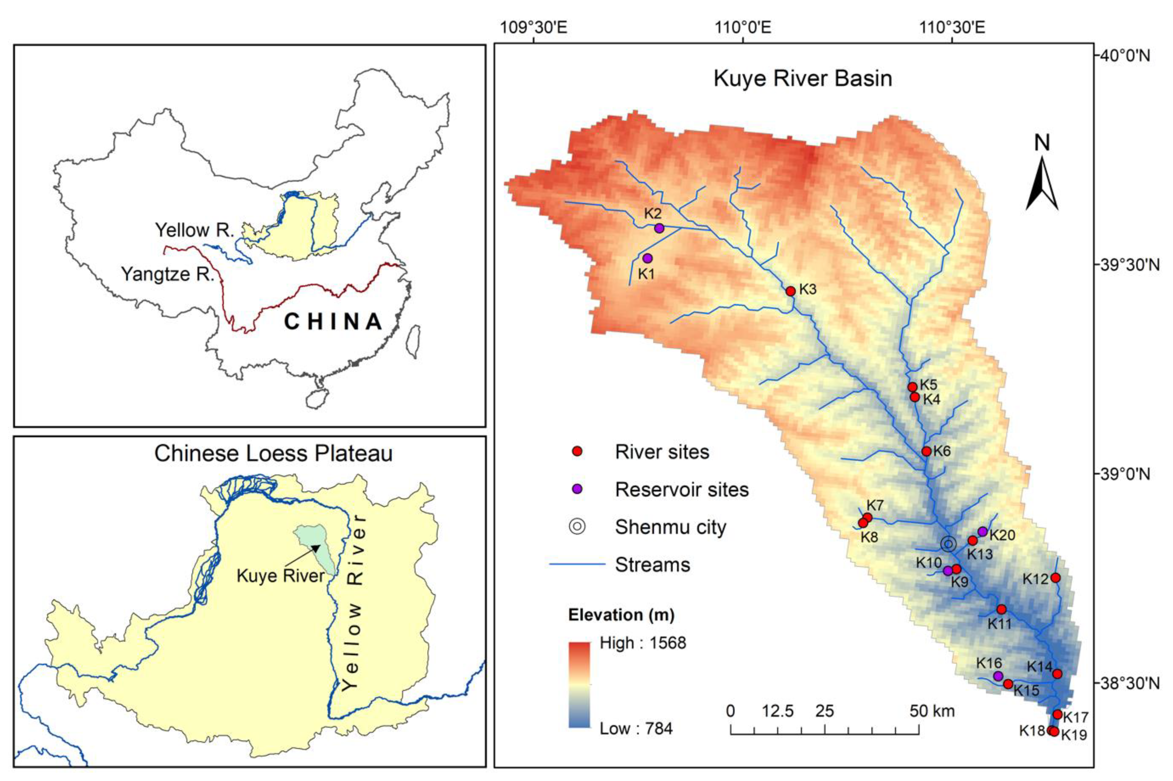
The Kuye River basin (KRB, 38.37–39.87° N, 109.43–110.81° E) is a medium-sized basin in the arid northern Chinese Loess Plateau and a major tributary of the YR (Figure 1). The mainstream length is 242 km, and the basin area is 8706 km2 with elevation ranging from 784 to 1568 m. The section from the headwater to Shenmu City is located in the upper reaches of the basin (Figure 1), where the main soil type is sandy soil. The middle-lower reaches of the basin are located southeast of Shenmu City and are predominantly covered with loess soils rich in carbonate. The long-term average annual precipitation in the KRB is 368.2 mm, with ~60% of the precipitation recorded between July and September. Consequently, the flow discharge varies significantly between the dry (October–May) and wet (June–September) seasons. The river basin has a freezing period of up to two months (from mid-December to the end of February). In recent years, there has been a noticeable increase in vegetation in the KRB due to ongoing afforestation, which have alleviated the long-standing soil erosion problem [21].
2.2. Field Measurement of Water-Quality Parameters and CO2 and CH4 Emissions
Field measurements were conducted in July (summer high-flow period), October (autumn) 2018, late March (spring), and June (summer low-flow period) 2019 in KRB. There were a total of 20 sampling sites, including 15 river sites and 5 reservoir sites (Figure 1). Sampling sites were located as far upstream as possible from urban and pollution sources so that the measurement results reflected the natural conditions to the greatest extent possible. The reservoir sites covered both the upper and lower reaches of the river basin, and the storage ranges between 1 × 10⁵ and 1 × 10⁶ m3. The age of the upstream reservoirs is 6–10 years, with a depth of 5–8 m and a surface area of 1.3–3.3 km2. The downstream reservoirs (5–12 m deep) are older than the upstream reservoirs, with an age of 10–20 years, and the water surface area varies from 0.01 to 0.05 km2.
All containers used for water sampling were sterilized prior to the field campaign, and they were rinsed three times before the water samples were collected. A total of 2 L of water at approximately 5 cm below the water surface was extracted at each sampling site and was stored in a refrigerator at 4 °C until analysis (within 1 week after sampling). Surface water quality variables, including pH, water temperature, and salinity, were measured using a Multi-3630 portable water-quality meter (WTW, Weilheim, Germany). The water-quality meter was calibrated with three pH buffer solutions (pH = 4.01, 7.00, and 10.01) before the beginning of each field campaign to ensure the accuracy of the pH measurement. The collected water samples were filtered through a 0.7 μm filter paper (Whatman GF/F), and total alkalinity was determined in the field through titration using 0.1 M HCl. The titration was repeated twice to ensure the error was within 5%. Since bicarbonate (HCO3−) ions in the YR can account for >96% of the total alkalinity [20], while the dissolved inorganic carbon (DIC) is mainly composed of HCO3−, total alkalinity was used in this study in lieu of DIC for analysis. Wind speed and air temperature were measured using Kestrel 2000 anemometer (Kestrel, Boothwyn, PA, USA). For the measurement of the dissolved organic carbon (DOC) concentration, 40 mL of the filtered water samples were acidified with phosphoric acid to pH < 2. An Elementar vario total organic carbon (TOC) analyzer (Elementar, Langenselbold, Germany) was used to determine DOC with an error of <5%. Apart from the rivers in the summer high-flow period, an additional 500 mL of water samples were collected, with magnesium carbonate suspension added for chlorophyll-a (Chl-a) measurements. Chl-a was first extracted by using 10 mL 10% acetone solution and then measured with a UV-2600 spectrophotometer (Shimadzu, Kyoto, Japan) with an accuracy of ±0.01 μg L−1.
We deployed freely drifting floating chambers to measure the FCO2 [22]. The floating chamber has a volume of 10.77 L and a surface area of 0.10 m². The surface of the floating chamber was wrapped in aluminum foil to minimize the effect of solar radiation, and a thermometer was installed to record the temperature change in the floating chamber during the deployment. During the deployment, the floating chamber was connected to the Licor-7000 CO2 analyzer (LI-COR, Lincoln, NE, USA) through two rubber tubes to form a closed loop. When the air pressure in the floating chamber was equilibrated with the atmospheric pressure, the floating chamber was then put on the water surface and we initiated the recording of the CO2 concentration inside the chamber using the CO2 analyzer. Each measurement lasted for 10–15 min, and duplicate measurements were performed at each site to enhance the reliability of the results.
For the measurement of diffusive FCH4, the same chamber was placed on the water surface, and a three-way stopcock was used to allow the floating chamber to be isolated from the ambient air during the measurement. A syringe was connected to another three-way stopcock, and the air accumulated in the floating chamber was collected with 12-mL Exetainer® vials (Labco, Lampeter, UK) every 5 min for 15 min (four samples in total at each site). The concentration of CH4 was determined using a Nexis GC-2030 gas chromatograph (GC-FID/ECD, Shimadzu, Kyoto, Japan). The GC system was calibrated using a standard gas (20.7 ppm), and the precision based on duplicate samples was ±4%.
The surface water pCO2 was also measured using the headspace equilibrium method. The headspace bottle has a volume of 630 mL and was rinsed at least three times before the pCO2 measurement in the field. A 400 mL water sample was collected afterward so that the ratio of water to headspace was 1.74:1. The bottle was then shaken vigorously for about 2 min to equilibrate the CO2 between water and air before connecting it to the Licor-7000 CO2 analyzer. The measurements of pCO2 were done in triplicate to ensure that the error was within 5%. Finally, the actual pCO2 was computed based on the CO2 solubility constant, headspace ratio, and the change in pH of the water before and after headspace equilibration [23].
2.3. Calculation of CO2- and CH4-Emission Flux
The diffusive GHG-exchange flux (F), including CO2 (FCO2, in mmol m−2 d−1) and CH4 (FCH4, in µmol m−2 d−1) at the water-air interface, was determined by changes in the GHG concentration in the floating chamber
where represents the slope of pCO2 (μatm s−1) or pCH4 (natm s−1) in the floating chamber, V is the volume of the floating chamber (m3), R is the gas constant (m3 atm K−1 mol−1), T is the temperature in the floating chamber (K), and S is the area of water in contact with the floating chamber (m²).
The calculation of k (cm h−1) was achieved based on the GHGs concentration differences between water and the ambient air, in addition to the F value obtained during the floating chamber deployment:
where and denote the GHGs concentrations in water and the ambient air, respectively. The value of k was then normalized to k600 for a Schmidt number (Sc) of 600 when the temperature is 20 °C for the purpose of facilitating the comparison of results with different publications,
where Sc is the temperature-dependent Sc of CO2 and CH4 at a given temperature calculated by Equations (4) and (5), respectively. The coefficient n was determined by the wind speed, which was either −1/2 or −2/3, when the wind speed was higher than 3.6 m s−1 or lower than 3.6 m s−1, respectively.
To determine the ebullitive CH4 flux, we employed the method developed by Campeau et al. (2014) [24]. Briefly, it assumed that all FCO2 were diffusive, while ebullitive FCO2 was non-existent. Based on , , and kCO2, the k for CH4 and the theoretical diffusive flux of CH4 was computed, and the divergence between FTCH4 and FCH4 was ascribed to the ebullitive FCH4.
2.4. Statistical Analyses
The statistical analyses were performed by IBM SPSS Statistics (Version 27). The two-sample independent t-test was conducted to test for the differences in the mean of variables between the upper reaches and the middle-lower reaches and between the rivers and reservoirs. One-way ANOVA followed by Tukey’s post-hoc test was performed for examining the differences in mean among seasons. In search of the best model to explain the variation of pCO2 and CH4 emissions at the rivers and reservoirs, the potential explanatory environmental variables, including pH, DOC, DIC, dissolved oxygen (DO), water temperature, Chl-a, wind speed, season, and flow velocity (rivers only), were utilized during the model development process. A model was created separately for rivers and reservoirs. The best model was selected by the Akaike Information Criterion (AIC). The threshold of the p-value to be deemed as statistically significant for all statistical analyses was 0.05.
3. Results
3.1. Environmental and Water-Quality Factors
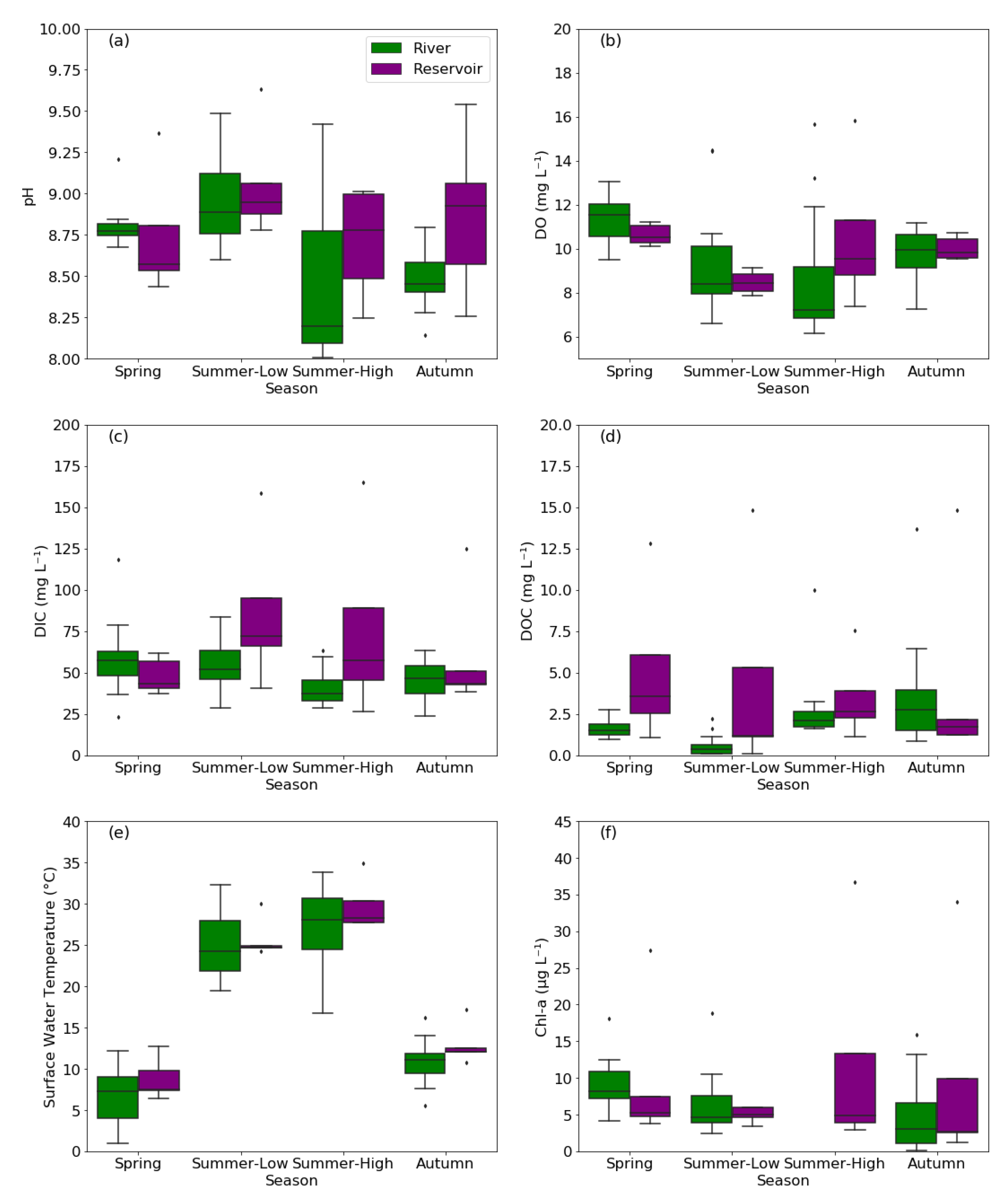
The major water-quality parameters of the KRB are summarized in Figure 2. The rivers were weakly alkaline, with the pH ranging from 8.0 to 9.5 (mean: 8.7, Figure 2a). The mean pH of rivers was the lowest in the summer high-flow period (8.4) and highest in the summer low-flow period (9.0). The water temperature varied significantly across the four sampling seasons (Figure 2e) and was significantly higher in summer (16.7–33.8 °C) than in autumn (5.5–16.2 °C) and spring (1.0–12.2 °C). The wind speed ranged from 0.1 to 2.0 m s−1, and there were no significant differences in flow velocity among seasons. The mean Chl-a concentration was 6.7 µg L−1 (Figure 2f) and exhibited obvious seasonal variation in the order: spring (9.1 µg L−1) > summer (6.2 µg L−1) > autumn (4.7 µg L−1). DOC concentration ranged from 0.1 to 13.7 mg L−1, with a mean value of 2.0 mg L−1. The mean DIC concentration was 53.9 mg L−1, with a range of 23.0 to 118.1 mg L−1 (Figure 2c). There were no significant differences in DOC and Chl-a concentration between the upper reaches and middle-lower reaches (p > 0.05, two-sample t-test).
For reservoirs, the pH was slightly higher than that of rivers (8.2–9.3, mean: 8.8, Figure 2a). The trends of water temperature and wind speed were consistent with those of the rivers. The DIC concentrations were slightly higher than those of the rivers, ranging from 26.5 to 101.4 mg L−1, with an overall mean value of 67.3 mg L−1 and higher concentrations in summer than in spring and autumn (Figure 2e). There were only significant differences between seasons for water temperature (p < 0.05, one-way ANOVA), while the pH, Chl-a concentration, DOC, DIC, and DO were not statistically different between seasons (p > 0.05, one-way ANOVA). The mean values of both DOC and DIC concentration in reservoirs (4.4 mg L−1 and 67.3 mg L−1, respectively, Figure 2d) were higher than that of the rivers (2.0 mg L−1 and 49.8 mg L−1, respectively, Figure 2c), and the differences were statistically significant (p < 0.05, Two-sample t-test). The annual mean reservoir Chl-a concentration was approximately 23% higher than that of the rivers. Notwithstanding, there was no significant difference of Chl-a between reservoirs and rivers after excluding the Chl-a data in summer high-flow period (t = 1.28, p = 0.21, two-sample t-test).
3.2. pCO2 and FCO2 in Rivers and Reservoirs
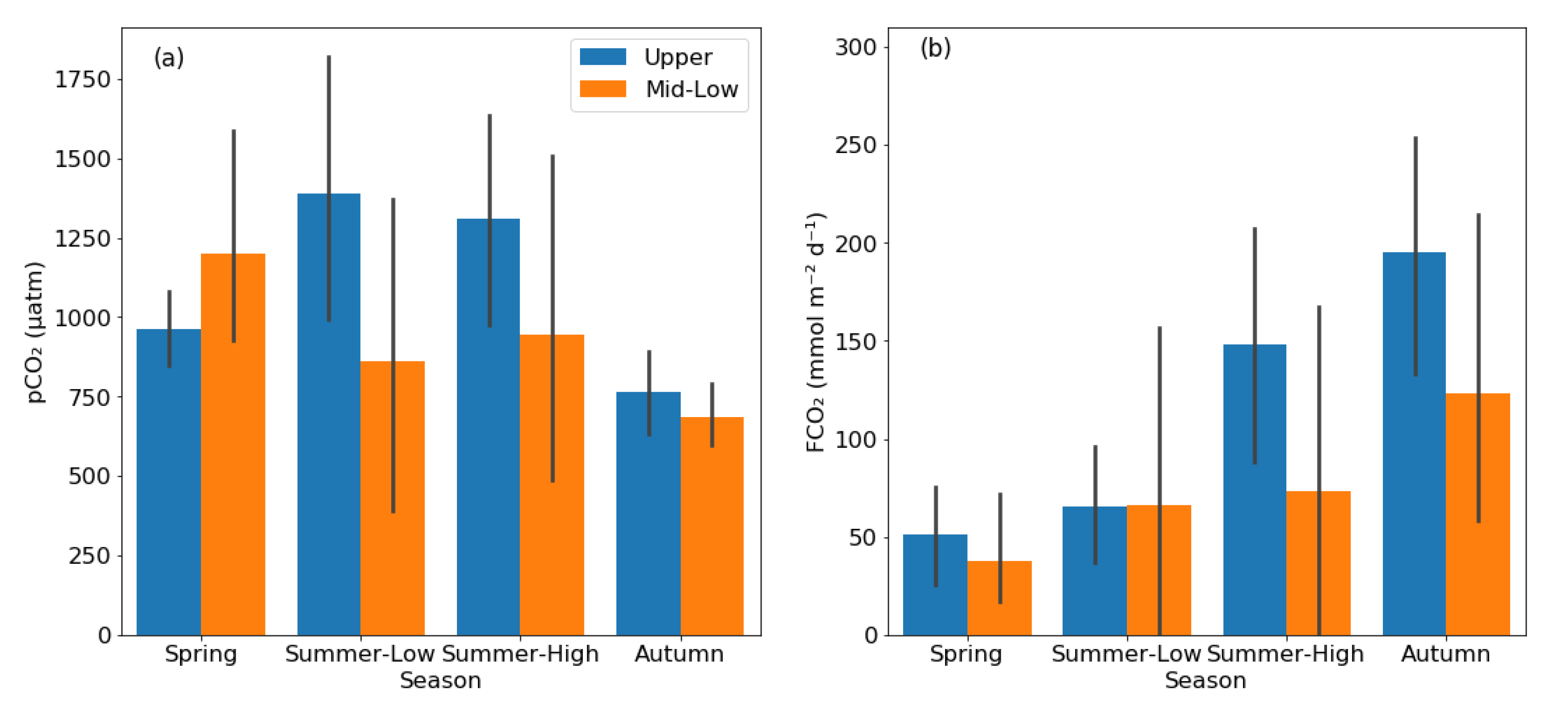
The rivers in the KRB were generally supersaturated with CO2. The stream water pCO2 varied from 43–2603 μatm, and the mean pCO2 was 1105 ± 426 μatm, 1074 ± 767 μatm, 1090 ± 707 μatm, and 716 ± 165 μatm in spring, summer low-flow period, summer high-flow period, and autumn, respectively (Figure 3a). Although there were no significant seasonal differences in pCO2 among seasons (p > 0.05; one-way ANOVA), the stream water pCO2 in autumn was more than 30% lower than that in the other three campaigns. The mean stream FCO2 was 43.0 ± 40.8, 66.1 ± 101.2, 103.1 ± 122.7, and 152.0 ± 122.4 mmol m−2 d−1 during spring, summer low-flow period, summer high-flow period, and autumn, respectively (Figure 3b). The FCO2 had statistically significant seasonal differences (p < 0.05, one-way ANOVA), and the post-hoc Tukey’s test indicated the FCO2 in autumn was significantly higher than spring. The overall mean stream FCO2 was 91.0 ± 108 mmol m−2 d−1.
pCO2 and FCO2 also showed significant differences between reaches (Figure 3a,b), mainly in the summer high-flow period and autumn. During the two seasons, although pCO2 was only about 30% higher in upper reaches (1036 ± 431 μatm) than in middle-lower reaches (815 ± 596 μatm), mean FCO2 (171.4 ± 83.7 mmol m−2 d−1) in upper reaches was higher than in middle-lower reaches (98.3 ± 137.8 mmol m−2 d−1) by about 70%. Considering the year-long measurement, pCO2 was higher in the upper reaches (1105 ± 441 μatm) than in middle-lower reaches (923 ± 650 μatm), and FCO2 was also higher in the upper reaches (114.8 ± 86.0 mmol m−2 d−1) than in the middle and lower reaches (75.2 ± 119.1 mmol m−2 d−1).
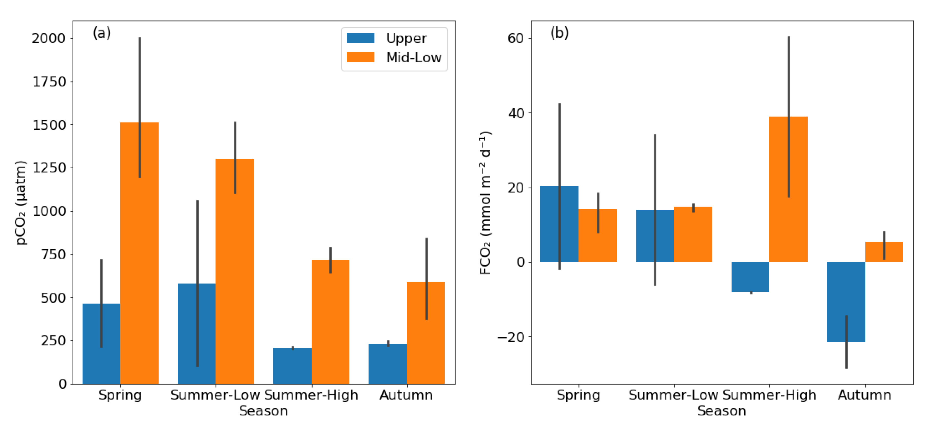
Compared to rivers, reservoirs exhibited different patterns in pCO2 and FCO2 (Figure 4). The pCO2 ranged from 104–2001 μatm, with a mean value of 1092 ± 672 μatm, 1010 ± 537 μatm, 461 ± 300 μatm, and 447 ± 255 μatm during spring, summer low-flow period, summer high-flow period, and autumn, respectively. The reservoir pCO2 in the upper reaches (371 ± 332 μatm) were 65% lower than those in the middle-lower reaches (1056 ± 474 μatm), and the differences were statistically significant (p < 0.05, two-sample t-test). The FCO2 ranged from −28.2–60.3 mmol m−2 d−1, with mean value of 16.6 ± 16.4 mmol m−2 d−1, 14.4 ± 14.2 mmol m−2 d−1, 15.5 ± 32.3 mmol m−2 d−1, and −5.4 ± 15.7 mmol m−2 d−1 during spring, summer low-flow period, summer high-flow period, and autumn, respectively. The overall mean FCO2 was 10.0 ± 20.6 mmol m−2 d−1. Unlike rivers, which act as a carbon source throughout the year, the reservoirs acted as C sinks with negative mean FCO2 during autumn. The reservoirs located in the upper reaches had lower FCO2 values (1.2 ± 24.3 mmol m−2 d−1) than those located in the middle-lower reaches (16.4 ± 15.5 mmol m−2 d−1), although the differences between the two landscape types were not statistically significant (p = 0.11, two-sample t-test).
3.3. Diffusive and Ebullitive FCH4 in Rivers and Reservoirs
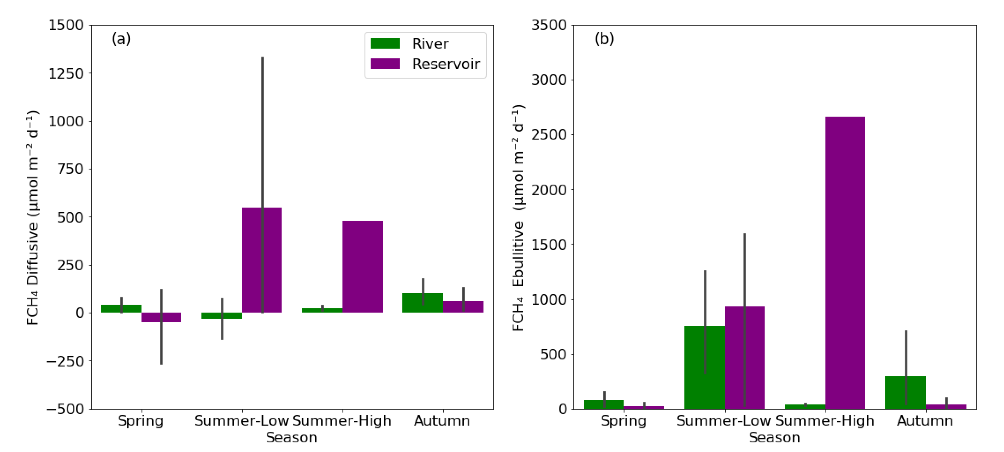
The average diffusive FCH4 in rivers and reservoirs were 29 ± 123 and 215 ± 439 µmol m−2 d−1, respectively (Figure 5a). The average ebullitive FCH4 in rivers and reservoirs were 323 ± 571 and 564 ± 934 µmol m−2 d−1, respectively (Figure 5b). The total FCH4 (sum of diffusive and ebullitive FCH4) were 352 ± 605 and 779 ± 1278 µmol m−2 d−1 in rivers and reservoirs, respectively.
The diffusive FCH4 did not exhibit significant seasonal differences for both reservoir (p = 0.36, one-way ANOVA) and rivers (p = 0.19, one-way ANOVA). However, both rivers and reservoirs occasionally had negative diffusive CH4 values in spring and the summer low-flow period. For rivers, the diffusive FCH4 did not exhibit statistically significant differences among seasons, while statistically significant differences were found (p < 0.05, one-way ANOVA). The Tukey’s post-hoc test further demonstrated that the ebullitive FCH4 during the summer low-flow period was significantly higher than that of spring and the summer high-flow period in rivers. For the reservoirs, the diffusive and ebullitive FCH4 during the summer-high were excluded for comparing seasonal trends, and both diffusive and ebullitive FCH4 did not have statistically significant differences. The mean ebullitive FCH4 in rivers was 82 ± 108, 756 ± 794, 38 ± 15, and 295 ± 533 µmol m−2 d−1 during spring, summer low-flow period, summer high-flow period, and autumn, respectively. Furthermore, the ebullitive FCH4 during the summer high-flow period (mean: 2660 µmol m−2 d−1) and summer low-flow period (mean: 934 ± 812 µmol m−2 d−1) was much higher than that of spring (19 ± 32 µmol m−2 d−1) and autumn (41 ± 51 µmol m−2 d−1) in reservoirs. Considering rivers and reservoirs together, the percentage of ebullitive FCH4 to total FCH4 was 77%, 89%, 82%, and 71% in spring, summer low-flow period, summer high-flow period, and autumn, respectively.
3.4. Estimates of pCO2 and FCH4 in Multiple Linear Regression Models
The selection processes of the multiple linear regression models suggested that the stream water pCO2 in the KRB was best explained by pH, DIC, and DO. pH and DO were negatively correlated while DIC was positively correlated with pCO2 (Table 1). A model including the three aforementioned variables explained 37% of the observed pCO2 variability. Regarding the reservoirs, the best model including wind speed and Chl-a as predictors explained 40% of the observed pCO2 variability. Both parameters were negatively associated with pCO2 (Table 1). For the total FCH4 variability, water temperature alone could explain 64% of the variability in reservoirs (Table 2). On the other hand, the environmental factors of pH, Chl-a, and wind speed can explain 40% of the variability of FCH4 in rivers (Table 2).
4. Discussion
4.1. Seasonal Differences of CO2 and CH4 Characteristics
Our works revealed that the stream water pCO2 during autumn was more than 300 ppm lower than that in the other seasons, while the pCO2 in the other three periods was relatively stable when considering mean values of upper and mid-lower reaches (Figure 3a). The largely equivalent pCO2 in the summer low-flow and high-flow periods implied that the potential dilution effect triggered by heavy rainfall events was likely to be insignificant in the KRB. In addition, the pCO2 values in spring were similar to those of summer despite the likely slower mineralization of organic C and CO2 production by microorganisms during spring when the temperature is lower [9]. We argue this might be due to the presence of a freezing period in the KRB, in which the ice cover might have effectively barred CO2 from being evaded across the air-water boundary during winter and led to the accumulation of large amounts of dissolved CO2 due to the decomposition and oxidation of organic matter in the water column under the ice [3,5]. In addition, the greater contribution of groundwater-derived CO2 in river water when precipitation is low in spring might also help explain this pattern [25]. As the temperature rose in spring and the ice cover gradually melted, an enormous amount of CO2 accumulated under the ice may be mobilized and delivered into the fluvial networks, translating into a significantly higher pCO2 during spring [26]. Alternatively, the significantly lower temperature in spring comparing to summer could have facilitated the dissolution of gases in water, which might have offset the effect of metabolism on pCO2 due to the lower temperatures. The higher pCO2 in summer than in autumn was proposed to be related to the higher flow discharge in summer and thus stronger terrestrial organic C inputs and mineralization of organic C [27]. Because the dilution effect on pCO2 is rather weak in this river basin, the above-mentioned factors may explain the higher pCO2 in river waters in summer than in autumn.
For the reservoirs, the relatively high pCO2 values during spring could be explained by the presence of ice cover during winter, as in the case of the rivers. A study covering 13 lakes and a reservoir in Québec, Canada showed that CO2 is usually accumulated and concentrated at the bottom [28]. When the ice melted, the previously accumulated CO2 at the reservoir bottom was released into the water column, resulting in the high pCO2 [26]. The lower value of pCO2 during the summer high-flow period and autumn was potentially driven by the stronger primary productivity caused by the autotrophs. The FCO2 and pCO2 had a statistically significant relationship in reservoirs (r = 0.46, p < 0.05) and rivers (r = 0.39, p < 0.05), indicating pCO2 can explain a considerable portion of variabilities in FCO2. It should be highlighted, however, that although the reservoir pCO2 during the summer low-flow period was approximately double that of during the summer high-flow period, the FCO2 during the two periods were highly similar (Figure 4). We argue this was likely attributed to the low wind speed during the summer low-flow period since the mean wind speed was only 0.3 m s−1, the lowest wind speed among the four periods. The diverging trend in pCO2 and FCO2 from summer to autumn might also be attributed to change in wind speed since the average wind speed during autumn was 107% higher than summer. Wind provides the energy to generate waves and is the main source of near-surface turbulence for lentic systems [29,30]. Hence, weak surface turbulence in the reservoirs would generally result in low k values that impact the magnitude of FCO2, which was consistent with previous studies that illustrated the importance of wind speed in governing the CO2 emission rates [30,31].
As for the seasonal variations of CH4 emissions, our data showed that the magnitude of ebullitive FCH4 and percentage of ebullitive FCH4 to total FCH4 was much higher during summer than spring and autumn, although it was the dominant pathway in all seasons. It was likely attributable to the exponential relationship between ebullitive FCH4 and water temperature. It has been reported that a threshold temperature of 25 °C exists for the methanogenesis in sediments and soils to have an exponential relationship with temperature [32]. A recent study in Swedish lakes suggested that the average CH4 formation rate with an increase of 10 °C in temperature was also several times higher when the temperature is 20–30 °C compared to 4–10 °C, suggesting much greater temperature sensitivity of CH4 formation under high-temperature environment [33]. Furthermore, a recent incubation experiment based on lake sediments also indicated that an increase of temperature by 2 °C could result in an increase of CH4 emission by 47–183% because methanogenesis is more sensitive to temperature than methanotrophy [34]. As the water temperature in most reservoirs and rivers in the KRB was well above 30 °C in summer, the CH4 production from the anoxic deep sediments and littoral sediments of these systems would likely be high [35], thus producing a disproportionate effect on CH4 emissions. The relatively higher percentage of ebullitive FCH4 to total FCH4 during summer was also consistent with the studies in ponds and lakes as well as subtropical rivers [36,37], which suggested that the ecosystem productivity is disproportionately more temperature-dependent for ebullition relative to diffusion. The formation of CH4 bubbles requires CH4 supersaturation in benthic sediments when the methanogenesis rate in sediments was greater than the rate of CH4 diffusing out of sediment [36]. Higher temperatures added to the differences between these two pathways, and accordingly, more CH4 would be emitted via the ebullition pathway.
4.2. Environmental Drivers of CO2 and CH4 Emissions
Our modelling found that the pH, DIC, and DO were the three environmental variables that could best elucidate the variability of stream water pCO2, while wind speed and Chl-a were the two most useful variables to account for the variability of pCO2 in reservoirs. It was no surprise that DO was a predictor in stream water pCO2 variability since respiration of aquatic organisms and the decomposition of terrestrially derived C will result in the consumption of oxygen and the release of CO2 into the water. Conversely, the primary productivity of autotrophs in water could potentially increase DO and decrease the value of pCO2 and thus the FCO2. This was in accordance with previous studies which indicated the intense community respiration in aquatic ecosystems could result in an elevated level of pCO2 and decreased DO [38,39].
In addition, pH was also a predictor of pCO2 in both rivers and reservoirs. Previous studies reported that when the surface water pH is above 7, the dissolved CO2 will be ionized into HCO3− and carbonate (CO32−) ions, thereby influencing the pCO2 through the buffering effect [40,41]. In contrast, the increase in pCO2 could favor the dissolution of carbonic acid, resulting a drop in pH. Our modeling at KRB is consistent with this general trend, as higher pH will lead to a decrease in pCO2. Although our model also shows a generally positive relationship between DIC and stream water pCO2, implying that the increase in pCO2 (a component of DIC) would lead to an increase in the overall DIC concentration, the very high pH may also lead to a relatively strong carbonate buffering effect, resulting in the decoupling of the relationship between the two variables in some individual cases. Taking the river site K15 (Figure 1) as an example, the pH was 9.4 during the summer low-flow period. Although its DIC concentration was remarkedly higher than the mean value of the rivers in the same period, the pCO2 was only 150 μatm. This result signified that most DIC might exist as HCO3− and CO32− ions, which is consistent with the theoretical carbonate system at high pH, i.e., enrichment of HCO3− and CO32− ions and depletion of dissolved CO2. Furthermore, it has been suggested the chemical enhancement of CO2 exchange in alkaline environments might have the possibility to elevate the FCO2, and a more accurate assessment of carbon fluxes might be achieved if it is taken into account [42].
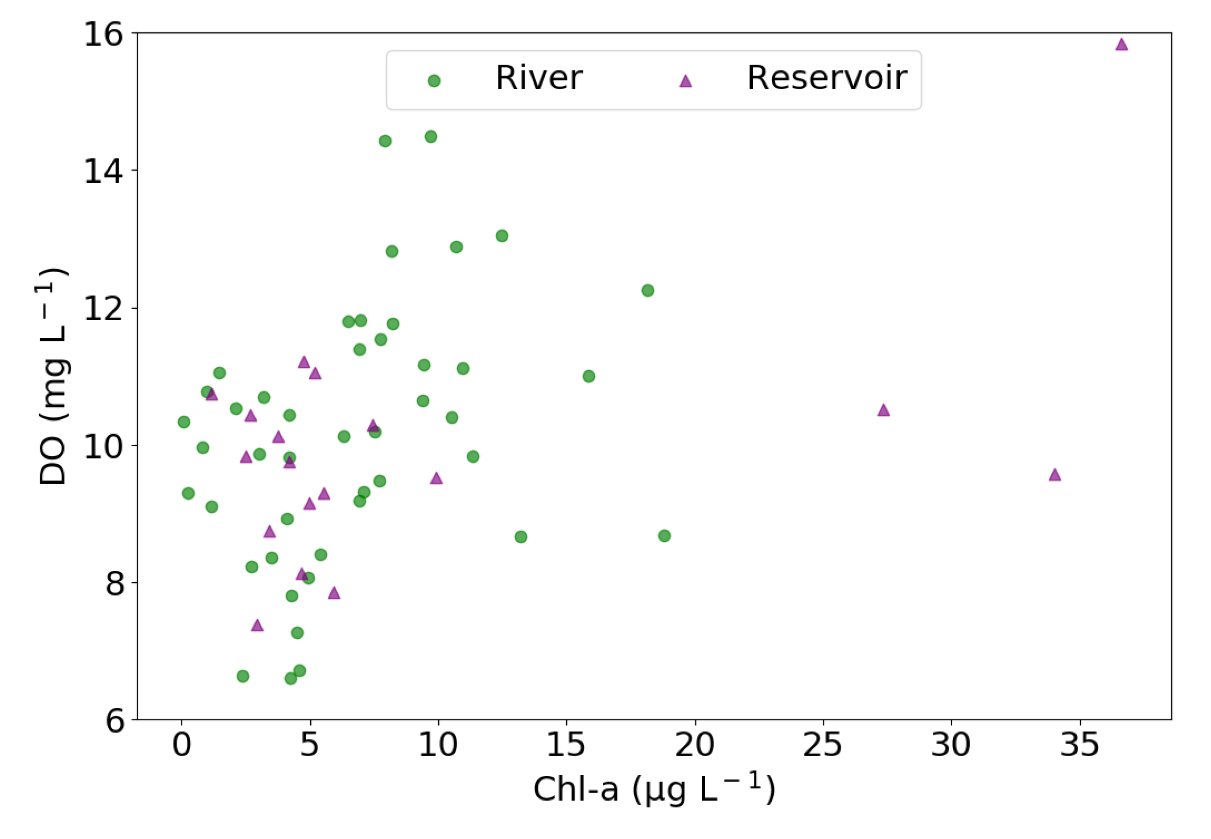
The inclusion of Chl-a as a predictor in the model for reservoir pCO2 reflected the importance of the primary productivity in controlling the CO2 dynamics in the KRB, since autotrophs can utilize vast quantities of CO2 through photosynthetic activities [43]. Accordingly, there was a negative connection between pCO2 with Chl-a. This argument was further corroborated by the statistically significant positive relationship between DO and Chl-a concentration at both reservoir (r = 0.55, p < 0.05, Figure 6) and rivers (r = 0.35, p < 0.05, Figure 6), implying that the elevated DO level was probably driven by strong primary productivity. Intense primary productivity of autotrophs in aquatic systems can result in the undersaturation of pCO2 relative to the atmospheric level [44], as observed here during summer and autumn (Figure 4a). Additionally, the model indicated an inverse relationship between reservoir pCO2 and wind speed. This inverse relationship is likely because the higher wind speed promoted higher k values in lentic waters, which in turn enhanced the outgassing of CO2 into the atmosphere and ultimately lowered the pCO2 in reservoirs when the reservoirs were supersaturated with pCO2, which is the majority of cases [45].
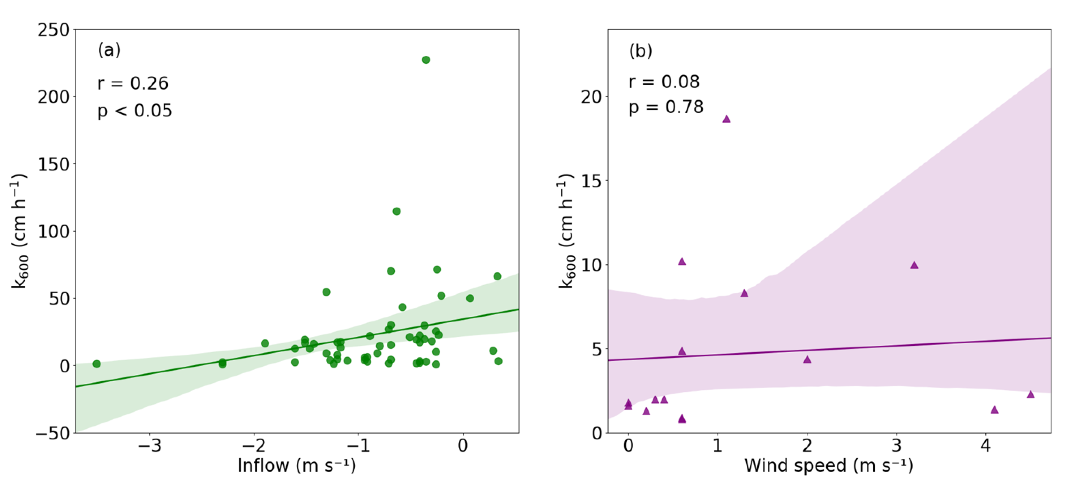
Our field results indicated a statistically significant positive correlation between k600 and the natural log-transformed flow velocity at the rivers (r = 0.26, p < 0.05, Figure 7a), suggesting that an increase in flow velocity caused higher k values, which in turn increased the magnitude of FCO2 and FCH4. This result was consistent with previous studies conducted in streams and rivers that indicated that flow velocity is an important factor regulating gas-transfer velocities [12,46]. For streams, the main source of turbulence comes from the shear stress triggered by the friction generated between the flowing water with the rough surface at the bottom [12,47,48]. As the flow velocity increases, there would be intensified stress generated from the streambed, thus translating the shear stress to the increased turbulence at the air-water boundary and facilitating gas diffusion [48,49]. Furthermore, there was no statistically significant positive correlation between k600 and the wind speed at the rivers (r = 0.01, p = 0.94), which was also in conformity with earlier studies that suggested that the near-surface turbulence in streams is relatively insensitive to wind [49].
There was a positive relationship between k600 and wind speed, although the relationship was not statistically significant (r = 0.08, p = 0.78, Figure 7b). This concurred with previous measurement and modeling results that postulated a positive association between wind speed and k600, because higher wind speeds can promote gas exchange through the transmission of energy from wind to waves [11,13,47,50]. However, prior studies have shown that other meteorological factors such as precipitation can also exert kinetic energy on the water surface and are capable of generating turbulence [31,50,51]. When the wind speed is low and hence the effect of wind stress not significant, precipitation may become the dominant factor in determining the k value. As the wind speeds recorded at the reservoirs were also low with a mean value of only 1.3 m s−1, the possibility that other meteorological variables such as precipitation in regulating the k600 values in reservoir waters could not be ruled out, thus attenuating the relationship between k600 and wind speed.
Regarding CH4 emissions, water temperature was clearly a determinant of the magnitude of the CH4 emitted to the atmosphere in reservoirs because of the exponential relationship of water temperature with ebullitive FCH4. The further inclusion of DOC as a predictor in the model will only increase the explanatory power (r2) slightly from 0.64 to 0.65 but will increase the model’s AIC and thus make it a less desirable model for predicting the FCH4. Although it has been reported that DOC is the substrate for the production of CH4 and hence the two parameters were likely to have a positive association [52], we found that in our study area, periods with high temperature were also the time when torrential rain occurred more frequently to enrich the DOC content in the water. Thus, we argue that the high degree of overlapping of the two parameters is the cause of a relatively low relative importance of DOC compared to temperature. This is consistent with previous studies that showed the absence of correlation between CH4 and DOC [32]. Although our model indicated the water temperature is the most important determinant of CH4 emissions, other factors, such as the increased rainfall and existence of anoxia environment in benthic sediment, might also favor the production of CH4 in some ecosystems [53]. Therefore, these parameters can also be considered and included in similar models in future studies.
Compared to reservoirs, the available data on environmental parameters were less capable of explaining the CH4 variation at the rivers since three parameters (pH, Chl-a, and wind speed) could only explain 40% of the FCH4 variability. pH was a perceivable factor affecting the magnitude of FCH4 because the activities of methanogens were sensitive to pH [54]. The depth of the river water column was significantly shallower than that of reservoirs, so we consider that wind-generated turbulence enhanced water reaeration [55], which increased DO concentrations and made it more difficult to develop and sustain an anaerobic environment at the bottom of the stream, ultimately leading to a negative correlation between wind speed and FCH4. Regarding the Chl-a, we postulate the observed positive relationship occurred since some oxygen-tolerant methanogens may exploit the substrate released by autotrophs to generate methane via hydrogenotrophic methanogenesis [32,56]. The fact that the water temperature was not a parameter included in the model for rivers was quite remarkable, and this signifies that the potential differences in CH4 controls between riverine and lacustrine sites warrant more in-depth investigations.
4.3. Comparison of C Emissions with Other Regions and Its Implications
The riverine FCO2 values in the arid KRB were comparable to the results observed in streams situated in boreal regions and China [57,58,59] while lower than that of stream networks in a number of subtropical and tropical regions [8,38,60] (Table 3). The FCO2 recorded in the reservoirs of the KRB was also in a similar magnitude to a number of lakes and reservoirs located in temperate and boreal North America and Europe as well as subtropical India [17,31,61] and fell within the range of FCO2 reported in subtropical lakes in China [59] but was comparatively lower than that of the studies focused on the reservoirs and lakes in the subtropical and tropical regions [62,63,64] (Table 3).
As for CH4 emissions, the rivers in the arid KRB had the same order of magnitude of FCH4 in a boreal stream network [15], while the magnitude of FCH4 in streams in Québec and major rivers in China was a few times higher than that obtained in this study [58,59] (Table 3). Concerning the reservoir FCH4 of the KRB, its magnitude was similar to the Three Gorges Dam, the average value of global temperate reservoirs, and subtropical lakes in China [59,62,65] (Table 3) but lower than that of tropical and subtropical reservoirs [62,64] (Table 3). These differences might be due to differences in the timing of sampling or the environment of the sampling sites or perhaps the techniques used in quantifying GHG fluxes [62]. In addition, ebullitive flux was realized to be a major component of FCH4 in numerous inland water systems, but the appearance of bubbles on the water surface is episodic and stochastic, which renders tremendous difficulties in the accurate determination of FCH4 [66,67]. Thus, continuous monitoring of GHG emissions at more sampling sites across different climate zones and dedicated monitoring of ebullitive FCH4 emissions is warranted.
Overall, the riverine FCO2 in the arid KRB was higher than that in the reservoirs, and the FCH4 accounts for a bigger share of the total C flux in reservoirs, in line with the overall tendency drawn from previous surveys (Table 3). This difference is due to the generally stronger turbulence of the river, which inhibits the development of an anaerobic environment conducive for CH4 emission [59]. By considering the differential global warming potential (GWP) between CO2 and CH4, i.e., 34 for CH4 and 1 for CO2 over a 100-year period, the mean GHG (CO2 and CH4 combined) emission rate in the reservoirs and rivers were 0.86 g CO2-eq m−2 d−1 and 4.20 g CO2-eq m−2 d−1, respectively, with CH4 accounting for 49% and 4.5% of the total CO2-eq of the two gases, respectively, indicating a higher percentage of GHGs released in the form of CH4 in reservoirs. This finding is also consistent with a study covering multiple Chinese reservoirs under different climate conditions, where it found that CH4 accounted for 79% of the total CO2-eq [68].
In order to cope with the increasing demand for electricity and water stemming from economic development, a growing number of reservoirs and impoundments have been built on rivers [69], significantly altering the geomorphology and thus riverine C cycle processes. Reservoirs might have the potential to emit more CO2 than natural lakes because the inundated terrestrial environment may have a stronger metabolism than natural lake sediments, while DOC released from ecosystems such as forests may be more labile [28,70]. Our study also found that the construction and operation of reservoirs are likely to change the physicochemical characteristics of river-water bodies. For instance, the importance of flow velocity to the C emission of the whole catchment is likely to decrease after an increasing number of river sections were turned into impoundments, rendering the potential to modulate the C exchange rate or even the flux direction of the entire basin. The contribution of CH4 emissions from reservoirs has been determined to be greater than that from rivers, and it has also been suggested that the CO2 emissions will progressively decrease after a reservoir is built, but the CH4 emissions will gradually increase over time [71]. Therefore, an expansion in the number of reservoirs may modulate the relative importance of different greenhouse gases to the Earth’s climate system for a given basin. This illustrates that, when assessing the regional-scale C budget, considering only the C exchange in fluvial systems while neglecting lacustrine systems will likely result in high uncertainty in the overall C evasion flux estimation. Hence, future studies on regional C balance must consider the differential C exchange rates and discrepancies in the GHG composition for both fluvial and lacustrine systems.
5. Conclusions
This study involved high-frequency measurements of GHG dynamics in the arid KRB. The riverine FCO2 was characterized by significant seasonal variability due to changes in the water-quality parameters, such as DO and pH, as well as hydrological variables such as flow velocity. For reservoirs, the FCO2 exhibited a different seasonal pattern than that of rivers, as the highest and lowest FCO2 was registered during spring and autumn, respectively, and several reservoirs can sometimes act as a C sinks. The best models derived from several environmental variables, e.g., the carbonate system, DO, DOC, and Chl-a, were capable of accounting for up to almost 40% of the variability in pCO2 in rivers and reservoirs. Flow velocity was found to be affecting the magnitude of k in rivers, while the effect of wind speed on k was insignificant. The best model explained more than 60% and almost 40% of the variability in FCH4 in reservoirs and rivers, respectively, in the studied basin. CH4 emissions were also much higher in summer likely because of the established exponential relationship between CH4 emission and temperature. A majority of FCH4 existed in the form of ebullition, accounting for >70% of the total CH4 flux in each season. Our field campaigns also demonstrated the significance of reservoirs in the CH4 emissions, accounting for almost half of the combined CO2-eq of CO2 and CH4. In order to accurately quantify the C budget at the basin scale, the differences in C dynamics between rivers and reservoirs need to be recognized, and both types of water bodies need to be covered during the sampling procedures. The construction of new impoundments can affect the C dynamics within a basin and the characteristics of reservoirs, such as age and the type of ecosystem inundated, might also affect the magnitude of GHG emitted.
Author Contributions
Conceptualization, H.S. and L.R.; data acquisition, H.S., B.L. and L.R.; data analysis and visualization, C.-N.C. and H.S.; writing, C.-N.C. and H.S.; supervision and funding acquisition, L.R. All authors have read and agreed to the published version of the manuscript.
Funding
This study was financially supported by the National Natural Science Foundation of China (Grant: 41807318), the Research Grants Council of Hong Kong (Grants: 17300619 and 27300118), and the Hui Oi-Chow Trust Fund (Grants: 201801172006).
Institutional Review Board Statement
Not applicable.
Informed Consent Statement
Not applicable.
Data Availability Statement
The data in this study are available from the corresponding authors upon request.
Acknowledgments
The publication fee was paid by the Grant 41807318.
Conflicts of Interest
The authors declare no conflict of interest.
References
- Cole, J.J.; Prairie, Y.T.; Caraco, N.F.; McDowell, W.H.; Tranvik, L.J.; Striegl, R.G.; Duarte, C.M.; Kortelainen, P.; Downing, J.A.; Middelburg, J.J.; et al. Plumbing the Global Carbon Cycle: Integrating Inland Waters into the Terrestrial Carbon Budget. Ecosystems 2007, 10, 172–185. [Google Scholar] [CrossRef] [Green Version]
- Battin, T.J.; Luyssaert, S.; Kaplan, L.A.; Aufdenkampe, A.K.; Richter, A.; Tranvik, L.J. The boundless carbon cycle. Nat. Geosci. 2009, 2, 598–600. [Google Scholar] [CrossRef]
- Wallin, M.B.; Grabs, T.; Buffam, I.; Laudon, H.; Ågren, A.; Öquist, M.G.; Bishop, K. Evasion of CO2 from streams–The dominant component of the carbon export through the aquatic conduit in a boreal landscape. Glob. Chang. Biol. 2013, 19, 785–797. [Google Scholar] [CrossRef] [PubMed]
- Raymond, P.A.; Hartmann, J.; Lauerwald, R.; Sobek, S.; McDonald, C.; Hoover, M.; Butman, D.; Striegl, R.; Mayorga, E.; Humborg, C.; et al. Global carbon dioxide emissions from inland waters. Nature 2013, 503, 355–359. [Google Scholar] [CrossRef] [Green Version]
- Teodoru, C.R.; del Giorgio, P.A.; Prairie, Y.T.; Camire, M. Patterns in pCO2 in boreal streams and rivers of northern Quebec, Canada. Glob. Biogeochem. Cycles 2009, 23. [Google Scholar] [CrossRef]
- Reiman, J.H.; Xu, Y.J. Diel Variability of pCO2 and CO2 Outgassing from the Lower Mississippi River: Implications for Riverine CO2 Outgassing Estimation. Water 2019, 11. [Google Scholar] [CrossRef] [Green Version]
- Striegl, R.G.; Dornblaser, M.M.; McDonald, C.P.; Rover, J.R.; Stets, E.G. Carbon dioxide and methane emissions from the Yukon River system. Glob. Biogeochem. Cycles 2012, 26. [Google Scholar] [CrossRef]
- Richey, J.E.; Melack, J.M.; Aufdenkampe, A.K.; Ballester, V.M.; Hess, L.L. Outgassing from Amazonian rivers and wetlands as a large tropical source of atmospheric CO2. Nature 2002, 416, 617–620. [Google Scholar] [CrossRef] [PubMed]
- AcuÑA, V.; Wolf, A.; Uehlinger, U.; Tockner, K. Temperature dependence of stream benthic respiration in an Alpine river network under global warming. Freshw. Biol. 2008, 53, 2076–2088. [Google Scholar] [CrossRef]
- Marx, A.; Dusek, J.; Jankovec, J.; Sanda, M.; Vogel, T.; van Geldern, R.; Hartmann, J.; Barth, J.A.C. A review of CO2 and associated carbon dynamics in headwater streams: A global perspective. Rev. Geophys. 2017, 55, 560–585. [Google Scholar] [CrossRef]
- Wanninkhof, R. Relationship between wind speed and gas exchange over the ocean. J. Geophys. Res. Ocean. 1992, 97, 7373–7382. [Google Scholar] [CrossRef]
- Raymond, P.A.; Zappa, C.J.; Butman, D.; Bott, T.L.; Potter, J.; Mulholland, P.; Laursen, A.E.; McDowell, W.H.; Newbold, D. Scaling the gas transfer velocity and hydraulic geometry in streams and small rivers. Limnol. Oceanogr. Fluids Environ. 2012, 2, 41–53. [Google Scholar] [CrossRef]
- Wanninkhof, R. Relationship between wind speed and gas exchange over the ocean revisited. Limnol. Oceanogr. Methods 2014, 12, 351–362. [Google Scholar] [CrossRef]
- Beaulieu, J.J.; DelSontro, T.; Downing, J.A. Eutrophication will increase methane emissions from lakes and impoundments during the 21st century. Nat. Commun. 2019, 10. [Google Scholar] [CrossRef] [Green Version]
- Crawford, J.T.; Striegl, R.G.; Wickland, K.P.; Dornblaser, M.M.; Stanley, E.H. Emissions of carbon dioxide and methane from a headwater stream network of interior Alaska. J. Geophys. Res. Biogeosci. 2013, 118, 482–494. [Google Scholar] [CrossRef]
- Maeck, A.; DelSontro, T.; McGinnis, D.F.; Fischer, H.; Flury, S.; Schmidt, M.; Fietzek, P.; Lorke, A. Sediment Trapping by Dams Creates Methane Emission Hot Spots. Environ. Sci. Technol. 2013, 47, 8130–8137. [Google Scholar] [CrossRef]
- Sobek, S.; DelSontro, T.; Wongfun, N.; Wehrli, B. Extreme organic carbon burial fuels intense methane bubbling in a temperate reservoir. Geophys. Res. Lett. 2012, 39. [Google Scholar] [CrossRef] [Green Version]
- DelSontro, T.; Beaulieu, J.J.; Downing, J.A. Greenhouse gas emissions from lakes and impoundments: Upscaling in the face of global change. Limnol. Oceanogr. Lett. 2018, 3, 64–75. [Google Scholar] [CrossRef] [PubMed]
- Spawn, S.A.; Dunn, S.T.; Fiske, G.J.; Natali, S.M.; Schade, J.D.; Zimov, N.S. Summer methane ebullition from a headwater catchment in Northeastern Siberia. Inland Waters 2015, 5, 224–230. [Google Scholar] [CrossRef]
- Ran, L.; Lu, X.X.; Yang, H.; Li, L.; Yu, R.; Sun, H.; Han, J. CO2 outgassing from the Yellow River network and its implications for riverine carbon cycle. J. Geophys. Res. Biogeosci. 2015, 120, 1334–1347. [Google Scholar] [CrossRef]
- Fu, B.; Wang, S.; Liu, Y.; Liu, J.; Liang, W.; Miao, C. Hydrogeomorphic Ecosystem Responses to Natural and Anthropogenic Changes in the Loess Plateau of China. Annu. Rev. Earth Planet. Sci. 2017, 45, 223–243. [Google Scholar] [CrossRef]
- Ran, L.; Li, L.; Tian, M.; Yang, X.; Yu, R.; Zhao, J.; Wang, L.; Lu, X.X. Riverine CO2 emissions in the Wuding River catchment on the Loess Plateau: Environmental controls and dam impoundment impact. J. Geophys. Res. Biogeosci. 2017, 122, 1439–1455. [Google Scholar] [CrossRef]
- Müller, D.; Warneke, T.; Rixen, T.; Müller, M.; Jamahari, S.; Denis, N.; Mujahid, A.; Notholt, J. Lateral carbon fluxes and CO2 outgassing from a tropical peat-draining river. Biogeosci. 2015, 12, 5967–5979. [Google Scholar] [CrossRef] [Green Version]
- Campeau, A.; Lapierre, J.-F.; Vachon, D.; del Giorgio, P.A. Regional contribution of CO2 and CH4 fluxes from the fluvial network in a lowland boreal landscape of Québec. Glob. Biogeochem. Cycles 2014, 28, 57–69. [Google Scholar] [CrossRef] [Green Version]
- Hotchkiss, E.R.; Hall Jr, R.O.; Sponseller, R.A.; Butman, D.; Klaminder, J.; Laudon, H.; Rosvall, M.; Karlsson, J. Sources of and processes controlling CO2 emissions change with the size of streams and rivers. Nat. Geosci. 2015, 8, 696–699. [Google Scholar] [CrossRef]
- Denfeld, B.A.; Wallin, M.B.; Sahlée, E.; Sobek, S.; Kokic, J.; Chmiel, H.E.; Weyhenmeyer, G.A. Temporal and spatial carbon dioxide concentration patterns in a small boreal lake in relation to ice-cover dynamics. Boreal Environ. Res. 2015, 20, 679–692. [Google Scholar]
- Paquay, F.S.; Mackenzie, F.T.; Borges, A.V. Carbon dioxide dynamics in rivers and coastal waters of the “big island” of Hawaii, USA, during baseline and heavy rain conditions. Aquat. Geochem. 2007, 13, 1–18. [Google Scholar] [CrossRef]
- Brothers, S.M.; Prairie, Y.T.; del Giorgio, P.A. Benthic and pelagic sources of carbon dioxide in boreal lakes and a young reservoir (Eastmain-1) in eastern Canada. Glob. Biogeochem. Cycles 2012, 26. [Google Scholar] [CrossRef]
- Read, J.S.; Hamilton, D.P.; Desai, A.R.; Rose, K.C.; MacIntyre, S.; Lenters, J.D.; Smyth, R.L.; Hanson, P.C.; Cole, J.J.; Staehr, P.A.; et al. Lake-size dependency of wind shear and convection as controls on gas exchange. Geophys. Res. Lett. 2012, 39. [Google Scholar] [CrossRef] [Green Version]
- Gålfalk, M.; Bastviken, D.; Fredriksson, S.; Arneborg, L. Determination of the piston velocity for water-air interfaces using flux chambers, acoustic Doppler velocimetry, and IR imaging of the water surface. J. Geophys. Res. Biogeosci. 2013, 118, 770–782. [Google Scholar] [CrossRef] [Green Version]
- Cole, J.J.; Caraco, N.F. Atmospheric exchange of carbon dioxide in a low-wind oligotrophic lake measured by the addition of SF6. Limnol. Oceanogr. 1998, 43, 647–656. [Google Scholar] [CrossRef] [Green Version]
- Xing, Y.; Xie, P.; Yang, H.; Ni, L.; Wang, Y.; Rong, K. Methane and carbon dioxide fluxes from a shallow hypereutrophic subtropical Lake in China. Atmos. Environ. 2005, 39, 5532–5540. [Google Scholar] [CrossRef]
- Duc, N.T.; Crill, P.; Bastviken, D. Implications of temperature and sediment characteristics on methane formation and oxidation in lake sediments. Biogeochemistry 2010, 100, 185–196. [Google Scholar] [CrossRef]
- Sepulveda-Jauregui, A.; Hoyos-Santillan, J.; Martinez-Cruz, K.; Walter Anthony, K.M.; Casper, P.; Belmonte-Izquierdo, Y.; Thalasso, F. Eutrophication exacerbates the impact of climate warming on lake methane emission. Sci. Total Environ. 2018, 636, 411–419. [Google Scholar] [CrossRef] [PubMed]
- Bastviken, D.; Cole, J.J.; Pace, M.L.; Van de Bogert, M.C. Fates of methane from different lake habitats: Connecting whole-lake budgets and CH4 emissions. J. Geophys. Res. Biogeosci. 2008, 113. [Google Scholar] [CrossRef]
- DelSontro, T.; Boutet, L.; St-Pierre, A.; del Giorgio, P.A.; Prairie, Y.T. Methane ebullition and diffusion from northern ponds and lakes regulated by the interaction between temperature and system productivity. Limnol. Oceanogr. 2016, 61, S62–S77. [Google Scholar] [CrossRef]
- Wu, S.; Li, S.; Zou, Z.; Hu, T.; Hu, Z.; Liu, S.; Zou, J. High Methane Emissions Largely Attributed to Ebullitive Fluxes from a Subtropical River Draining a Rice Paddy Watershed in China. Environ. Sci. Technol. 2019, 53, 3499–3507. [Google Scholar] [CrossRef]
- Wang, X.; He, Y.; Yuan, X.; Chen, H.; Peng, C.; Zhu, Q.; Yue, J.; Ren, H.; Deng, W.; Liu, H. pCO2 and CO2 fluxes of the metropolitan river network in relation to the urbanization of Chongqing, China. J. Geophys. Res. Biogeosci. 2017, 122, 470–486. [Google Scholar] [CrossRef]
- Zhai, W.; Dai, M.; Cai, W.-J.; Wang, Y.; Wang, Z. High partial pressure of CO2 and its maintaining mechanism in a subtropical estuary: The Pearl River estuary, China. Mar. Chem. 2005, 93, 21–32. [Google Scholar] [CrossRef]
- Duvert, C.; Bossa, M.; Tyler, K.J.; Wynn, J.G.; Munksgaard, N.C.; Bird, M.I.; Setterfield, S.A.; Hutley, L.B. Groundwater-Derived DIC and Carbonate Buffering Enhance Fluvial CO2 Evasion in Two Australian Tropical Rivers. J. Geophys. Res. Biogeosci. 2019, 124, 312–327. [Google Scholar] [CrossRef]
- Stets, E.G.; Butman, D.; McDonald, C.P.; Stackpoole, S.M.; DeGrandpre, M.D.; Striegl, R.G. Carbonate buffering and metabolic controls on carbon dioxide in rivers. Glob. Biogeochem. Cycles 2017, 31, 663–677. [Google Scholar] [CrossRef]
- Finlay, K.; Vogt, R.J.; Bogard, M.J.; Wissel, B.; Tutolo, B.M.; Simpson, G.L.; Leavitt, P.R. Decrease in CO2 efflux from northern hardwater lakes with increasing atmospheric warming. Nature 2015, 519, 215–218. [Google Scholar] [CrossRef]
- Zang, C.; Huang, S.; Wu, M.; Du, S.; Scholz, M.; Gao, F.; Lin, C.; Guo, Y.; Dong, Y. Comparison of Relationships Between pH, Dissolved Oxygen and Chlorophyll a for Aquaculture and Non-aquaculture Waters. WaterAirSoil Pollut. 2011, 219, 157–174. [Google Scholar] [CrossRef]
- Crawford, J.T.; Loken, L.C.; Stanley, E.H.; Stets, E.G.; Dornblaser, M.M.; Striegl, R.G. Basin scale controls on CO2 and CH4 emissions from the Upper Mississippi River. Geophys. Res. Lett. 2016, 43, 1973–1979. [Google Scholar] [CrossRef] [Green Version]
- Morales-Pineda, M.; Cózar, A.; Laiz, I.; Úbeda, B.; Gálvez, J.Á. Daily, biweekly, and seasonal temporal scales of pCO2 variability in two stratified Mediterranean reservoirs. J. Geophys. Res. Biogeosci. 2014, 119, 509–520. [Google Scholar] [CrossRef]
- Maurice, L.; Rawlins, B.G.; Farr, G.; Bell, R.; Gooddy, D.C. The Influence of Flow and Bed Slope on Gas Transfer in Steep Streams and Their Implications for Evasion of CO2. J. Geophys. Res. Biogeosci. 2017, 122, 2862–2875. [Google Scholar] [CrossRef] [Green Version]
- Raymond, P.A.; Cole, J.J. Gas Exchange in Rivers and Estuaries: Choosing a Gas Transfer Velocity. Estuaries 2001, 24, 312–317. [Google Scholar] [CrossRef]
- Ulseth, A.J.; Hall, R.O.; Boix Canadell, M.; Madinger, H.L.; Niayifar, A.; Battin, T.J. Distinct air–water gas exchange regimes in low- and high-energy streams. Nat. Geosci. 2019, 12, 259–263. [Google Scholar] [CrossRef]
- Beaulieu, J.J.; Shuster, W.D.; Rebholz, J.A. Controls on gas transfer velocities in a large river. J. Geophys. Res. Biogeosci. 2012, 117. [Google Scholar] [CrossRef]
- Ho, D.T.; Veron, F.; Harrison, E.; Bliven, L.F.; Scott, N.; McGillis, W.R. The combined effect of rain and wind on air–water gas exchange: A feasibility study. J. Mar. Syst. 2007, 66, 150–160. [Google Scholar] [CrossRef]
- Zappa, C.J.; Ho, D.T.; McGillis, W.R.; Banner, M.L.; Dacey, J.W.H.; Bliven, L.F.; Ma, B.; Nystuen, J. Rain-induced turbulence and air-sea gas transfer. J. Geophys. Res. Ocean. 2009, 114. [Google Scholar] [CrossRef] [Green Version]
- Mu, C.; Li, L.; Wu, X.; Zhang, F.; Jia, L.; Zhao, Q.; Zhang, T. Greenhouse gas released from the deep permafrost in the northern Qinghai-Tibetan Plateau. Sci. Rep. 2018, 8. [Google Scholar] [CrossRef] [PubMed]
- Brothers, S.; Köhler, J.; Attermeyer, K.; Grossart, H.P.; Mehner, T.; Meyer, N.; Scharnweber, K.; Hilt, S. A feedback loop links brownification and anoxia in a temperate, shallow lake. Limnol. Oceanogr. 2014, 59, 1388–1398. [Google Scholar] [CrossRef]
- Megonigal, J.P.; Hines, M.E.; Visscher, P.T. 10.8—Anaerobic Metabolism: Linkages to Trace Gases and Aerobic Processes. In Treatise on Geochemistry, 2nd ed.; Holland, H.D., Turekian, K.K., Eds.; Elsevier: Oxford, UK, 2014; pp. 273–359. [Google Scholar]
- Haider, H.; Ali, W.; Haydar, S. Evaluation of various relationships of reaeration rate coefficient for modeling dissolved oxygen in a river with extreme flow variations in Pakistan. Hydrol. Process. 2013, 27, 3949–3963. [Google Scholar] [CrossRef]
- Tang, K.W.; McGinnis, D.F.; Frindte, K.; Brüchert, V.; Grossart, H.-P. Paradox reconsidered: Methane oversaturation in well-oxygenated lake waters. Limnol. Oceanogr. 2014, 59, 275–284. [Google Scholar] [CrossRef] [Green Version]
- Huotari, J.; Haapanala, S.; Pumpanen, J.; Vesala, T.; Ojala, A. Efficient gas exchange between a boreal river and the atmosphere. Geophys. Res. Lett. 2013, 40, 5683–5686. [Google Scholar] [CrossRef]
- Rasilo, T.; Hutchins, R.H.S.; Ruiz-González, C.; del Giorgio, P.A. Transport and transformation of soil-derived CO2, CH4 and DOC sustain CO2 supersaturation in small boreal streams. Sci. Total Environ. 2017, 579, 902–912. [Google Scholar] [CrossRef] [PubMed]
- Kumar, A.; Yang, T.; Sharma, M.P. Greenhouse gas measurement from Chinese freshwater bodies: A review. J. Clean. Prod. 2019, 233, 368–378. [Google Scholar] [CrossRef]
- Li, S.; Lu, X.X.; Bush, R.T. CO2 partial pressure and CO2 emission in the Lower Mekong River. J. Hydrol. 2013, 504, 40–56. [Google Scholar] [CrossRef]
- Kumar, A.; Sharma, M.P. Assessment of risk of GHG emissions from Tehri hydropower reservoir, India. Hum. Ecol. Risk Assess. Int. J. 2016, 22, 71–85. [Google Scholar] [CrossRef]
- St. Louis, V.L.; Kelly, C.A.; Duchemin, É.; Rudd, J.W.M.; Rosenberg, D.M. Reservoir Surfaces as Sources of Greenhouse Gases to the Atmosphere: A Global Estimate: Reservoirs are sources of greenhouse gases to the atmosphere, and their surface areas have increased to the point where they should be included in global inventories of anthropogenic emissions of greenhouse gases. BioScience 2000, 50, 766–775. [Google Scholar]
- Wang, F.; Wang, B.; Liu, C.-Q.; Wang, Y.; Guan, J.; Liu, X.; Yu, Y. Carbon dioxide emission from surface water in cascade reservoirs–river system on the Maotiao River, southwest of China. Atmos. Environ. 2011, 45, 3827–3834. [Google Scholar] [CrossRef]
- Almeida, R.M.; Nóbrega, G.N.; Junger, P.C.; Figueiredo, A.V.; Andrade, A.S.; de Moura, C.G.B.; Tonetta, D.; Oliveira, E.S.; Araújo, F.; Rust, F.; et al. High Primary Production Contrasts with Intense Carbon Emission in a Eutrophic Tropical Reservoir. Front. Microbiol. 2016, 7. [Google Scholar] [CrossRef] [PubMed] [Green Version]
- Hao, Q.; Chen, S.; Ni, X.; Li, X.; He, X.; Jiang, C. Methane and nitrous oxide emissions from the drawdown areas of the Three Gorges Reservoir. Sci. Total Environ. 2019, 660, 567–576. [Google Scholar] [CrossRef] [PubMed]
- DelSontro, T.; McGinnis, D.F.; Wehrli, B.; Ostrovsky, I. Size Does Matter: Importance of Large Bubbles and Small-Scale Hot Spots for Methane Transport. Environ. Sci. Technol. 2015, 49, 1268–1276. [Google Scholar] [CrossRef] [PubMed]
- Linkhorst, A.; Hiller, C.; DelSontro, T.; Azevedo, G.M.; Barros, N.; Mendonça, R.; Sobek, S. Comparing methane ebullition variability across space and time in a Brazilian reservoir. Limnol. Oceanogr. 2020, 65, 1623–1634. [Google Scholar] [CrossRef]
- Kumar, A.; Yang, T.; Sharma, M.P. Long-term prediction of greenhouse gas risk to the Chinese hydropower reservoirs. Sci. Total Environ. 2019, 646, 300–308. [Google Scholar] [CrossRef]
- Zarfl, C.; Lumsdon, A.E.; Berlekamp, J.; Tydecks, L.; Tockner, K. A global boom in hydropower dam construction. Aquat. Sci. 2015, 77, 161–170. [Google Scholar] [CrossRef]
- Brothers, S.M.; del Giorgio, P.A.; Teodoru, C.R.; Prairie, Y.T. Landscape heterogeneity influences carbon dioxide production in a young boreal reservoir. Can. J. Fish. Aquat. Sci. 2012, 69, 447–456. [Google Scholar] [CrossRef]
- Teodoru, C.R.; Bastien, J.; Bonneville, M.-C.; del Giorgio, P.A.; Demarty, M.; Garneau, M.; Hélie, J.-F.; Pelletier, L.; Prairie, Y.T.; Roulet, N.T.; et al. The net carbon footprint of a newly created boreal hydroelectric reservoir. Glob. Biogeochem. Cycles 2012, 26. [Google Scholar] [CrossRef] [Green Version]
Figure 1.
Location map of the Kuye River Basin (KRB) with the sampling locations.

Figure 2.
The boxplots summarizing the water-quality parameters, including pH (a), DO (dissolved oxygen) (b), DIC (dissolved inorganic carbon) (c), DOC (dissolved organic carbon) (d), surface water temperature (e), and Chl-a (chlorophyll-a) (f), of rivers and reservoirs in the KRB. The dots represent the outliers, which are defined as the value lower than Q1-1.5 * interquartile range (IQR) or higher than Q3 + 1.5 * IQR. Summer-Low and Summer-High represent the summer low-flow period and summer high-flow period, respectively.

Figure 3.
The bar charts showing the pCO2 (a) and FCO2 (b) pattern in different seasons between the upper reaches and the middle-lower reaches in rivers. The grey error bars show the range of 95% confidence interval.
Figure 3.
The bar charts showing the pCO2 (a) and FCO2 (b) pattern in different seasons between the upper reaches and the middle-lower reaches in rivers. The grey error bars show the range of 95% confidence interval.

Figure 4.
The bar charts showing the pCO2 (a) and FCO2 (b) pattern in different seasons between the upper reaches and the middle-lower reaches in reservoirs. The grey error bars show the range of 95% confidence interval.
Figure 4.
The bar charts showing the pCO2 (a) and FCO2 (b) pattern in different seasons between the upper reaches and the middle-lower reaches in reservoirs. The grey error bars show the range of 95% confidence interval.

Figure 5.
The bar charts showing the diffusive FCH4 (a) and ebullitive FCH4 (b) pattern in different seasons between rivers and reservoirs. The grey error bars represent the range of 95% confidence interval. Note: The error bars for the diffusive and ebullitive FCH4 results were absent in the summer-high flow period because only one reservoir was sampled for CH4.

Figure 6.
Scatterplot showing the association between Chl-a and DO in rivers and reservoirs of the KRB. The r-value in rivers and reservoirs were 0.35 and 0.55, respectively, and were both statistically significant (p < 0.05).
Figure 6.
Scatterplot showing the association between Chl-a and DO in rivers and reservoirs of the KRB. The r-value in rivers and reservoirs were 0.35 and 0.55, respectively, and were both statistically significant (p < 0.05).

Figure 7.
Scatterplots showing the relationship between k600 and flow velocity (log-transformation) at the rivers (a) and k600 and wind speed at the reservoirs (b) after an outlier was omitted in the KRB. The shaded region represents the 95% confidence interval for the regression estimate using bootstrapping technique.


Table 1.
Parameter estimates for the best model developed for explaining the pCO2 in the rivers (R2 = 0.37) and reservoirs (R2 = 0.40).
Table 1.
Parameter estimates for the best model developed for explaining the pCO2 in the rivers (R2 = 0.37) and reservoirs (R2 = 0.40).
| Parameter | Estimate | Std. Error | t | p-Value | |
|---|---|---|---|---|---|
| River | Intercept | 5835.841 | 1785.974 | 3.268 | 0.002 |
| pH | −524.591 | 236.221 | −2.221 | 0.031 | |
| DO | −84.801 | 36.166 | −2.345 | 0.023 | |
| DIC | 10.833 | 3.953 | 2.740 | 0.008 | |
| Reservoir | Intercept | 1217.026 | 180.097 | 6.758 | 0.000 |
| Chl-a | −16.802 | 14.624 | −1.149 | 0.273 | |
| Wind speed | −176.315 | 93.382 | −1.888 | 0.083 |
Table 2.
Parameter estimates for the best model developed for explaining the total FCH4 in the rivers (R2 = 0.40) and reservoirs (R2 = 0.64).
Table 2.
Parameter estimates for the best model developed for explaining the total FCH4 in the rivers (R2 = 0.40) and reservoirs (R2 = 0.64).
| Parameter | Estimate | Std. Error | t | p-Value | |
|---|---|---|---|---|---|
| River | Intercept | −8.188 | 3.852 | −2.126 | 0.044 |
| pH | 0.977 | 0.442 | 2.212 | 0.037 | |
| Chl-a | 0.028 | 0.024 | 1.196 | 0.244 | |
| Windspeed | −0.315 | 0.179 | −1.762 | 0.091 | |
| Reservoir | Intercept | −1.165 | 0.579 | −2.013 | 0.079 |
| Temperature | 0.106 | 0.028 | 3.752 | 0.006 |
Table 3.
Estimates of FCO2 and FCH4 inland water systems in the KRB and other parts of the world.
| Water Type | Location | Climate Zone | FCO2 (mmol m−2 d−1) | FCH4 (µmol m−2 d−1) | References |
|---|---|---|---|---|---|
| Streams and rivers | Northwest China | Temperate | 91 | 352 | This study |
| China | Subtropical | 38–356 | 864–2938 | [59] | |
| Interior Alaska | Boreal | 450.1 | 631 | [15] | |
| Finland | Boreal | 83 | - | [57] | |
| Québec | Boreal | 66.3 | 2000 | [58] | |
| Chongqing | Subtropical | 447 | - | [38] | |
| Lower Mekong | Tropical | 195 | - | [60] | |
| Amazon | Tropical | 189 | - | [8] | |
| Lakes and reservoirs | Northwest China | Temperate | 10 | 779 | This study |
| New Hampshire | Boreal | 6.7–11.5 | - | [31] | |
| Brazil | Tropical | 42.5 | 2330 | [64] | |
| India | Subtropical | 18 | 4000 | [61] | |
| Switzerland | Temperate | 5.5 | 9820 | [17] | |
| China | Subtropical | 0.9–187 | 8.6–4840 | [59] | |
| Southwest China | Subtropical | 15–47.2 | - | [63] | |
| Three Gorges, China | Subtropical | - | 780 | [65] | |
| Global | Temperate | 32 | 1250 | [62] | |
| Global | Tropical | 79.5 | 18,800 | [62] |
Publisher’s Note: MDPI stays neutral with regard to jurisdictional claims in published maps and institutional affiliations. |
© 2021 by the authors. Licensee MDPI, Basel, Switzerland. This article is an open access article distributed under the terms and conditions of the Creative Commons Attribution (CC BY) license (https://creativecommons.org/licenses/by/4.0/).
Share and Cite
MDPI and ACS Style
Chan, C.-N.; Shi, H.; Liu, B.; Ran, L. CO2 and CH4 Emissions from an Arid Fluvial Network on the Chinese Loess Plateau. Water 2021, 13, 1614. https://doi.org/10.3390/w13121614
AMA Style
Chan C-N, Shi H, Liu B, Ran L. CO2 and CH4 Emissions from an Arid Fluvial Network on the Chinese Loess Plateau. Water. 2021; 13(12):1614. https://doi.org/10.3390/w13121614
Chicago/Turabian StyleChan, Chun-Ngai, Hongyan Shi, Boyi Liu, and Lishan Ran. 2021. "CO2 and CH4 Emissions from an Arid Fluvial Network on the Chinese Loess Plateau" Water 13, no. 12: 1614. https://doi.org/10.3390/w13121614
Note that from the first issue of 2016, this journal uses article numbers instead of page numbers. See further details here.