
A New Evolutionary Approach to Optimal Sensor Placement in Water Distribution Networks


1
Department of Computer Science, Systems and Communication, University of Milano-Bicocca, 20126 Milan, Italy
2
Department of Economics, Management and Statistics, University of Milano-Bicocca, 20126 Milan, Italy
*
Author to whom correspondence should be addressed.
Water 2021, 13(12), 1625; https://doi.org/10.3390/w13121625
Submission received: 26 April 2021
/
Revised: 4 June 2021
/
Accepted: 8 June 2021
/
Published: 9 June 2021
(This article belongs to the Section Urban Water Management)
Abstract
:The sensor placement problem is modeled as a multi-objective optimization problem with Boolean decision variables. A new multi objective evolutionary algorithm (MOEA) is proposed for approximating and analyzing the set of Pareto optimal solutions. The evaluation of the objective functions requires the execution of a hydraulic simulation model of the network. To organize the simulation results a data structure is proposed which enables the dynamic representation of a sensor placement and its fitness as a heatmap. This allows the definition of information spaces, in which the fitness of a placement can be represented as a matrix or, in probabilistic terms as a histogram. The key element in the new algorithm is this probabilistic representation which is embedded in a space endowed with a metric based on a specific notion of distance. Among several distances between probability distributions the Wasserstein (WST) distance has been selected: WST has enabled to derive new genetic operators, indicators of the quality of the Pareto set and criteria to choose among the Pareto solutions. The new algorithm has been tested on a benchmark water distribution network with two objective functions showing an improvement over NSGA-II, in particular for low generation counts, making it a good candidate for expensive black-box multi-objective optimization
1. Introduction
In this paper, a new algorithm is proposed for effectively and efficiently monitoring the spread of “effects” triggered by “events”. Many real-world problems fit into this general framework among which water distribution networks (WDNs), where sensing spots are sensors deployed at specific locations (i.e., nodes of the network), events are natural/intended contaminations and effects are spatio-temporal concentrations of the contaminant. This problem is usually known as optimal sensor placement (SP), where the goal is to optimize several objectives such as the amount of contaminated water, the number of inhabitants affected before detection, the detection time or the detection likelihood so that we faced with a multi-objective optimization problem (MOP). Due to potentially conflicting objectives, generally there is not a unique solution to multi-objective optimization problems but a set of solutions representing a trade-off between different objectives. This trade-off is characterized by the notion of dominance. The set of solutions representing the optimal (non-dominated) trade-offs between objectives is referred to as the Pareto set. Its image in the objectives space is called the Pareto front.
Exactly locating the complete Pareto set may be not possible, even for cheap objective functions: indeed, searching for an optimal sensor placement can be shown to be NP-hard. Therefore, even for mid-size networks, efficient approximate methods are required, among which evolutionary approaches are often used. The overall goal of multi objective optimization is to generate a good approximation of the Pareto set.
Time to detection is the key element in the optimal sensor placement problem upon whose value the other objectives of a sensor placement can be computed.
The main motivation of this study is that considering only the average value, over all the events, in an objective function could be misleading and entail significant risks. In order to mitigate this risk, the standard deviation of detection time is considered as a companion objective. The idea has been put forward in different papers [1,2].
Evaluating the above objective functions is expensive because it requires to perform the hydraulic simulation for a large set of contamination events, each one associated to a different location where the contaminant is injected.
Simulating the contaminant propagation allows to compute the minimum detection time (MDT) provided by a specific sensor placement (SP) over all the simulated events and its standard deviation.
Literature review: Evolutionary algorithms (EA) have a long history in multi-objective optimization, with many successful applications to sensor placement in water distribution networks (WDN’s) since the challenge “Battle of Water Sensors Networks” and many contributions have used NSGA-II [2,3,4]. More recently [5] considers the potential variations of model contamination probabilities within the WDN and introduce a regret based scalarization function based on the Chebyshev distance in the NSGA-II framework. An interesting methodology conditional value at risk (CVar) has been developed in [6], using four objectives and a criterion to choose from the Pareto solution set. Their approach considers quantiles to model extreme losses, in terms of detection time and affected population, caused by uncertain parameters. They also use a specific data structure storing all EPANET outputs for single point injection scenarios and extract from them multi-point water quality matrix based on superposition principles. A closely related paper to ours is [2] in which the conflicting objectives are the number of sensors (as a surrogate for their cost) and the risk of contamination defined as the product of the probability of not detecting the contaminant intrusion and the corresponding consequence expressed as the average volume of water consumed before detection. The algorithm NSGA-II is used to solve the MOP. Optimal sensor placement has been also addressed with methods from mathematical programming as in [7] which uses a mixed integer programming model solved by cPlex and a greedy randomized adaptive search procedure (GRASP) and [8] where a branch and bound sensor algorithm is proposed based on greedy heuristics and convex relaxation.
In this paper, the optimal sensor placement problem is modeled as a multi-objective optimization problem with Boolean decision variables and a new evolutionary algorithm for finding a good approximation of the Pareto set is proposed.
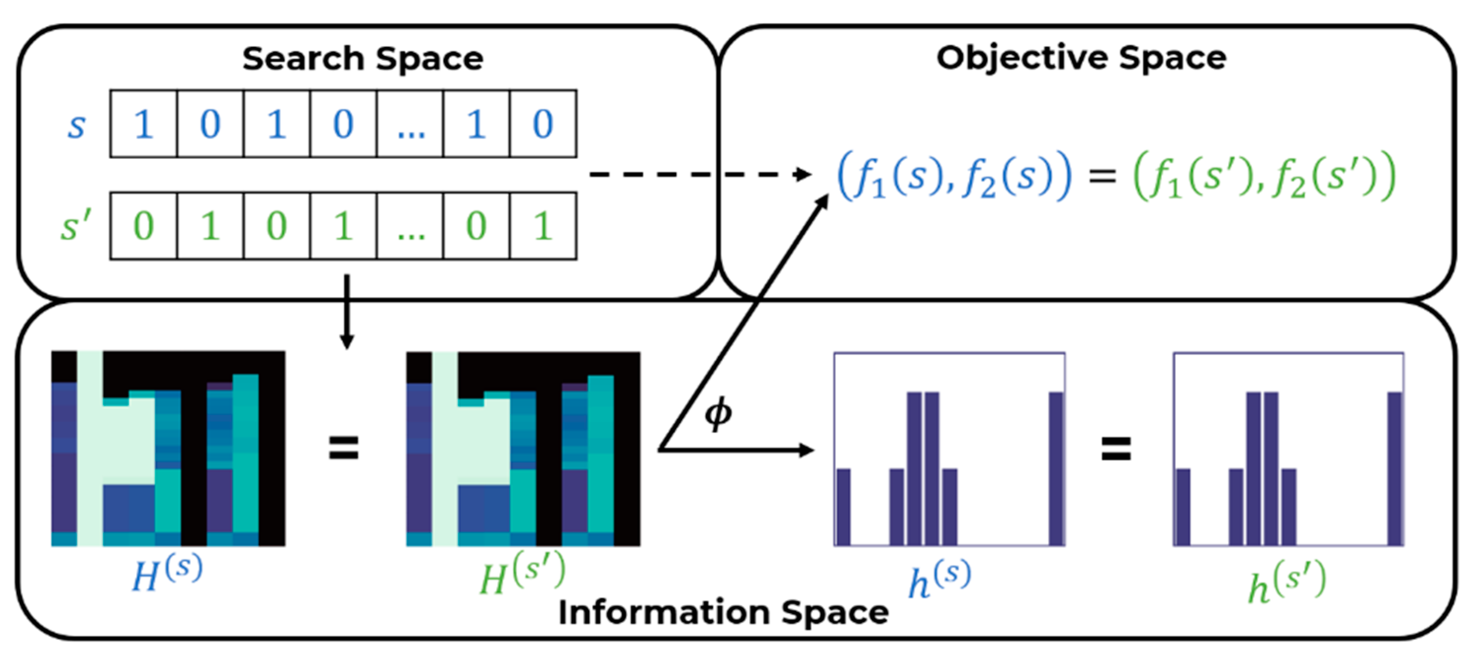
To organize the simulation results in a computationally efficient way a data structure is proposed collecting simulation outcomes for every SP which is particularly suitable for visualization and evolutionary optimization.
This data structure enables to visualize the dynamic representation of the spatio-temporal concentration of the contaminant and the detection time associated to a sensor placement. This structure is revealed through matrices represented by heat- maps which integrate a randomized set of contamination events.
Upon these heat-maps a mapping is built from the search space (where each SP is represented as a binary vector) into an information space, whose elements can be represented as a matrix or, as a histogram in the space of one-dimensional discrete probability distributions. The fitness of a sensor placement is represented probabilistically in the information space as the histogram of a discrete random variable.
The representation of a sensor placement as a histogram is the cornerstone of the new algorithm: it enables to measure the distance between sensor placements as a distance between distributions allowing a deep analysis of the search landscape and a significant speed-up in the optimization.
Among the many distances available the Wasserstein distance (WST) has been used in that provides a smooth and interpretable distance metric between distributions. This probabilistic representation has allowed to derive new genetic operators and indicators of the quality of the Pareto set.
Distinguishing features of the new algorithm MOEA/WST are in particular the selection operator which drives a more effective diversification and exploration among candidate solutions and a problem specific crossover operator which generates two “feasible by design” children from two feasible parents. This new algorithm, called multi-objective evolutionary algorithm-Wasserstein (MOEA-WST) has been tested on two benchmark and two real-world water distribution networks resulting in significant improvement over a standard algorithm both in terms of hypervolume improvement and coverage, in particular at low generation counts.
After the formulation of the problem in Section 2, Section 3 describes the specific data structure to organize the simulation results in a computationally efficient way which is also suitable for visualization and evolutionary optimization. The mathematical background is explained in two sections: Section 4 covers the methodological background of the probabilistic characterization of the search space, in particular the introduction of the Wasserstein distance. Section 5 covers the basic notions of Pareto analysis of multi-objective optimization and generalizes them in the context of the probabilistic representation. Section 6 leverages all the elements previously introduced into the design of the new algorithm MOEA/WST stressing the role of the new operators. The computational results are presented and discussed in Section 7. The last section “Conclusions” elaborates on the advantages of the algorithm and on how the probabilistic representation has allowed substantial improvements in terms of hypervolume and coverage, requiring a significantly lower number of generations. This makes MOEA/WST a good candidate for expensive multi-objective optimization problems.
2. Problem Formulation
We consider a graph We assume a set of possible locations for placing sensors, that is . Thus, a SP is a subset of sensor locations, with the subset’s size less or equal to depending on the available budget. An SP is represented by a binary vector whose components are if a sensor is located at node , otherwise. Thus, an SP is given by the nonzero components of .
For a WDN the vertices in represent junctions, tanks, reservoirs or consumption points, and edges in represent pipes, pumps, and valves.
Let denote the set of contamination events which must be detected by a sensor placement , and the impact measure associated to a contamination event a detected by the -th sensor.
A probability distribution is placed over possible contamination events associated to the nodes. In the computations we assume—as usual in the literature—a uniform distribution, but in general discrete distributions are also possible. In this paper, we consider as objective functions the detection time and its standard deviation.
We consider a general model of sensor placement, where is the “impact” of a sensor located at Node I when the contaminant has been introduced at Node a.
- is the probability for the contaminant to enter the network at Node .
- is the impact for a sensor located at Node to detect the contaminant introduced at Node .
- if , where is the first sensor detecting the contaminant injected at Node ; otherwise.
- is the budget available in terms of number of sensors.
In our study we assume that all the events have the same chance of happening, that is , therefore is:
where is the MDT of event .
As a measure of risk, we consider the standard deviation
This model can be specialized to different objective functions as: is the average over the contamination events of the detection time for each event. For each event and sensor placement the minimum detection time is defined as .
With the minimum time step at which concentration reaches or exceeds a given threshold for the event .
is the standard deviation of the sample average approximation of .
3. Simulation, Network and Event Data Description
3.1. WNTR
The Water Network Tool for Resilience (WNTR) [9] is a Python package designed to simulate and analyze resilience of WDNs. WNTR is based on EPANET 2.0, which is a tool to simulate flowing of drinking water constituents within a WDN.
The simulation is computationally costly as we need one execution for each contamination event.
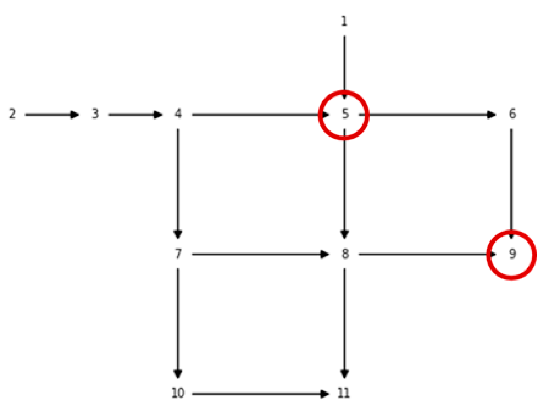
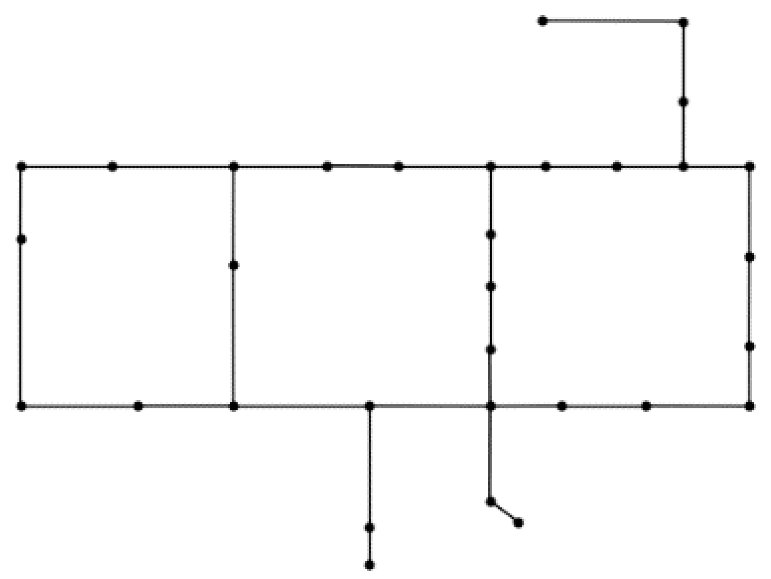
In our study, each simulation has been performed for 24 h, with a simulation step of 1 h. Assuming and (i.e., the most computationally demanding problem configuration) the time required to run a simulation for the synthetic example called Net1 (available with EPANET and WNTR, and whose associated graph is depicted in Figure 1) is 2 s. The simulation time scales linearly with the inverse of the simulation step. The detection threshold is 10% of the initial concentration.
3.2. Single Sensor and Sensor Placement Matrices
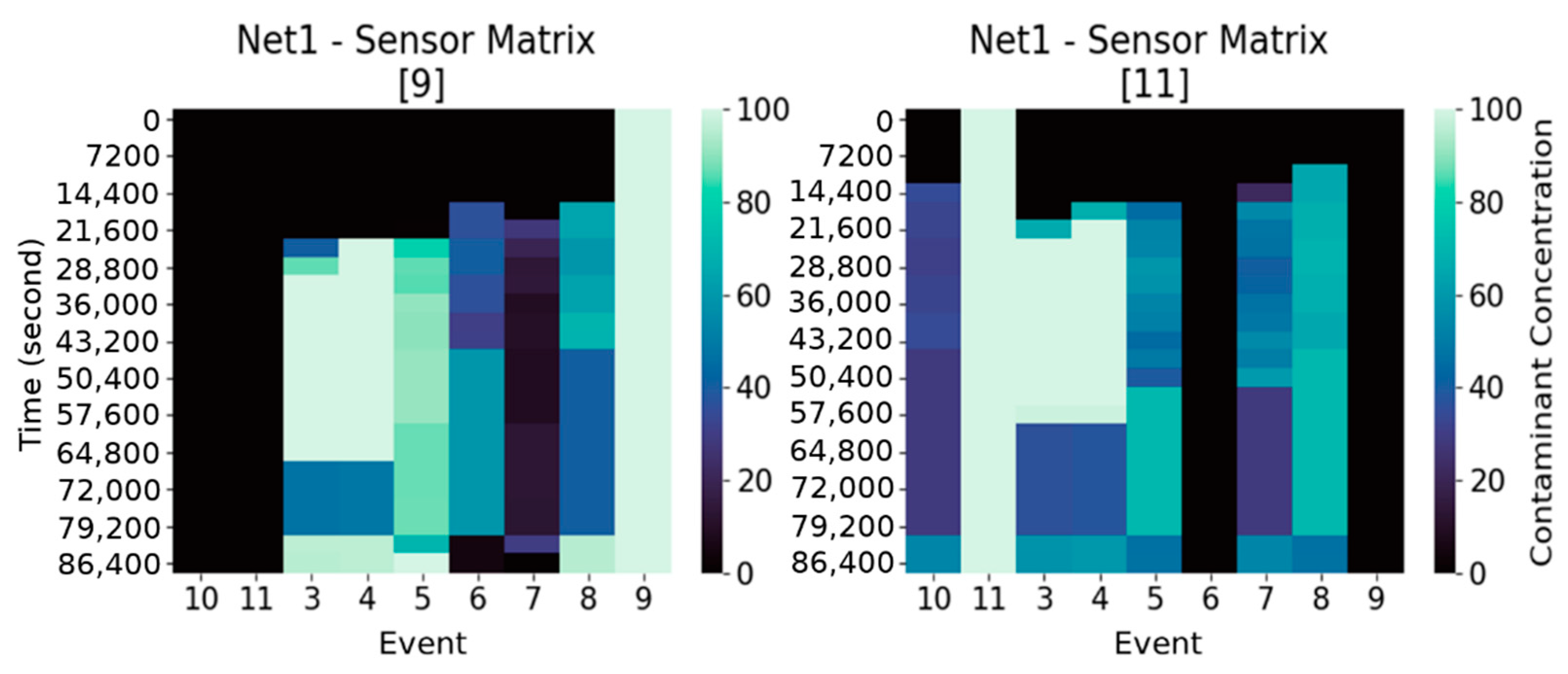
Denote with the so-called “sensor matrix” (Figure 2), with an index identifying the location where the sensor is deployed at. Each entry of , represents the concentration of the contaminant for the event at the simulation step , with .
Thus, in our study , and . Without loss of generality, we assume that the contaminant is injected at the beginning of the simulation (i.e., ).
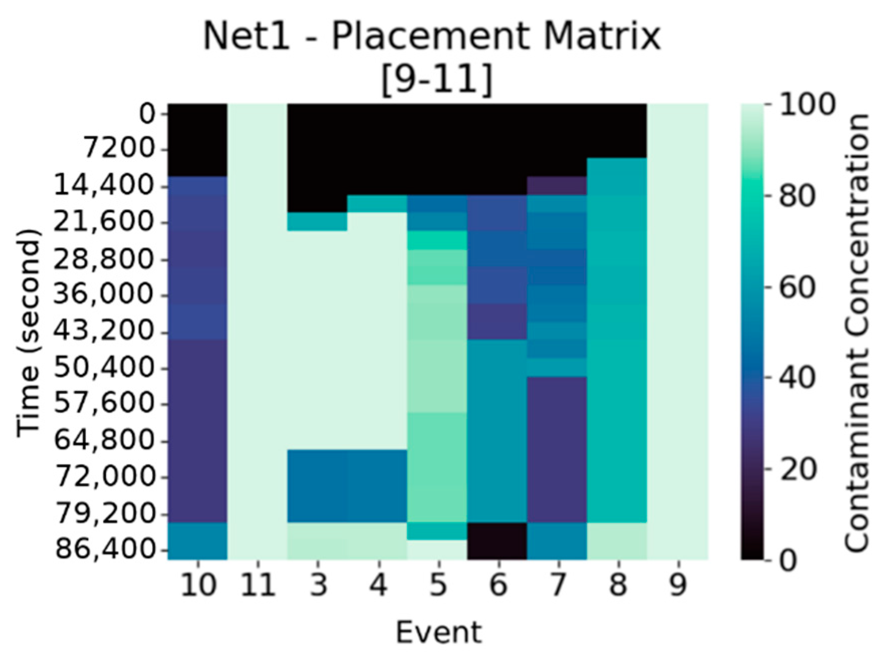
Analogously, a “sensor placement matrix” (Figure 3), is defined, where every entry represents the maximum concentration over those detected by the sensors in , for the event and at time step . Suppose to have a sensor placement consisting of sensors with associated sensor matrices , then is the matrix with entries .
There is a relation between and the associated more precisely, the columns of having maximum concentration at row (i.e., injection time) are those associated to events with injection occurring at the deployment locations of the sensors in .
Moreover, is the basic data structure on which MDT is computed. Indeed, we can now explicit the computation of in and : is the minimum time step at which concentration reaches or exceeds a given threshold for the scenario , that is .
4. The Probabilistic Characterization of the Search Space
The search space consists of all the possible SPs, given a set of possible locations for their deployment, and resulting feasible with respect to the constraints in (P). Formally, . In this section, sensor placements will be associated to a discrete probability distribution, specifically histograms, and a distance between them, namely the Wasserstein distance, will be introduced and briefly analyzed.
4.1. Histograms
In general terms a histogram is a function that counts the number of n observations of a random variable that fall into each of the disjoint categories (known as bins). Therefore, if k is the number of bins, the histogram satisfies the condition:
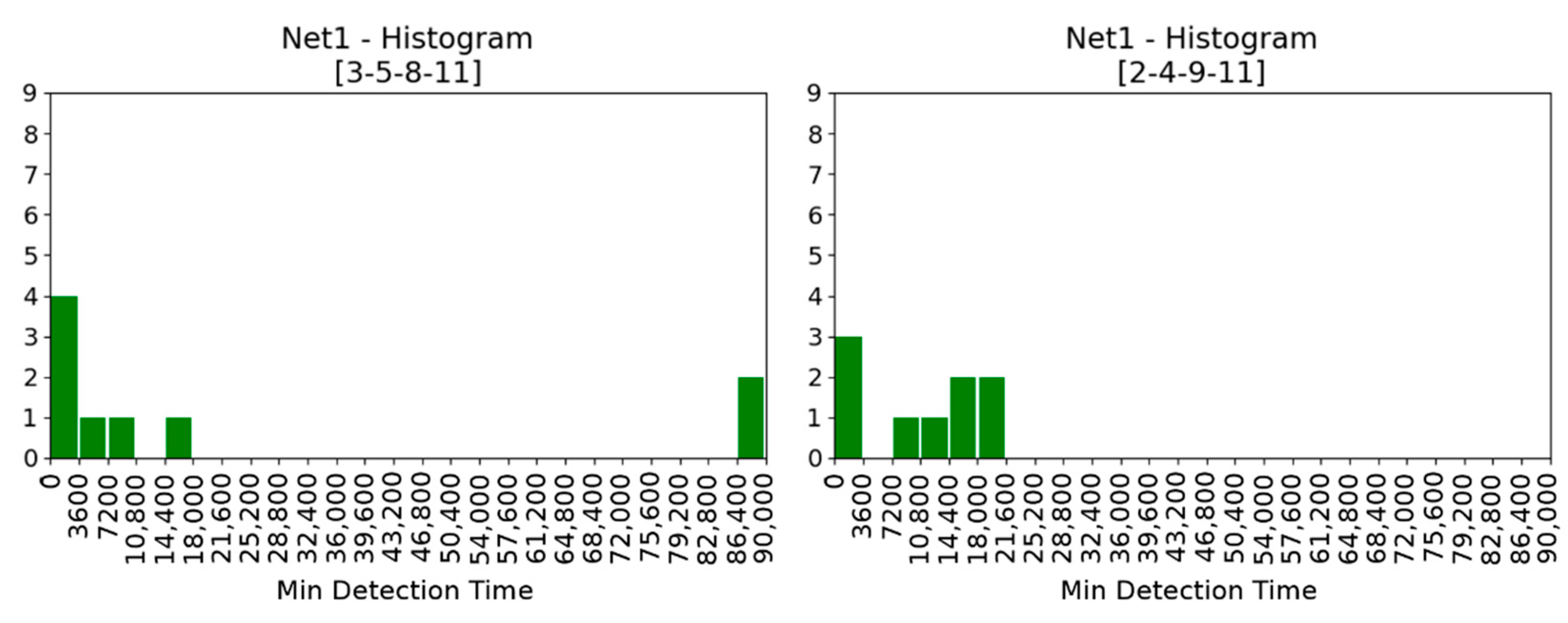
To construct a histogram, the first step is to “bin” the range of values—that is, divide the support of the random variable into a number of intervals—and then compute the “weight” of the bin counting how many values fall into each interval. The bins are usually specified as adjacent, consecutive, non-overlapping intervals and are usually of the same size. If bins are the time subintervals of the simulation horizon and the weights are the number of events detected in each time subinterval (or their relative frequency) the histogram obtained is a rich representation of the information in about a placement (Figure 4). We denote the time steps in the simulation where are equidistanced in the simulation time horizon . , , . We consider the discrete random variable where . cardinality is the number of contamination events, the bins are and . To each sensor placement we can associate not only the placement matrix but also the histogram whose bins are and weights are .
We have added an “extra” bin (86,400 to 90,000) whose weight represents number of contamination events which were undetected during the simulation up to 86,400. In this way .
The “ideal” placement is that in which || = |A|. The relation between SPs and histograms is many to one: one histogram can be associated to different SPs.
4.2. Wasserstein Distance
Let and be two continuous probability distributions. The Wasserstein () distance is a measure of the distance between and given by:
where denotes the set of all joint distributions whose marginals are respectively and .
In general terms, given two continuous random variables and whose joint distribution is known, then the marginal probability density function can be obtained by integrating the joint probability distribution, over , and vice versa. That is:
Therefore, the marginal distribution over adds up to and analogously . The formula can be easily specialized to the case of two discrete random variables, and . The marginal distribution of either variable—, given the joint probability distribution , is given by:
The expected cost averaged over all the pairs can be computed as:
The Wasserstein distance is also called earth mover’s (EM) distance from its informal interpretation as the minimum cost of moving and transforming a pile of sand in the shape of the probability distribution p to the shape of the distribution p′. The cost is quantified by the amount of sand moved times the moving distance.
If is the starting point and the destination the total amount of sand moved is and the traveling distance is and thus the cost is . One joint distribution describes one transport plan: intuitively indicates how much mass must be transported from to in order to transform the distribution into the distribution . The minimum among the costs of all sand moving solutions as the EM distance which is the cost of the optimal transport plan.
The Wasserstein (WST) distance fits in the framework of optimal transport theory. It can be traced back to the work of Gaspard Monge [10] and received its modern linear programming formulation by Lev Kantorovich [11]. Recently, the Wasserstein distance has become a key tool in image processing and machine learning, and it has been used also the generation of adversarial networks [12].
The formulation, computation and generalization of the WST distance require sophisticated mathematical models and raise challenging computational problems: important references are [13,14] which also gives an up-to-date survey of numerical methods. In the case of the sensor placement problem, the computation of WST reduces to the comparison of two 1-D histograms which can be done by simple sorting.
Among other probability distances, as Kullback–Leibler or Jensen–Shannon, WST has two key advantages. In addition, in the cases when the distributions are supported in different spaces, even without overlaps, WST can still provide a meaningful representation of the distance between distributions [15]. Another advantage of WST is its differentiability. Both points are illustrated in the following example [16].
Consider the uniform distribution on the unit interval. Let be the distribution of (0 on the axis and the random variable on the axis and .
- if and 0 if .
- if and 0 if .
- if and 0 if .
Therefore, Wasserstein provides a smooth measure which is useful for any optimization and learning process using gradient descent [16].
5. Multi-Objective Optimization in Search Space and Information Space
5.1. Search Space and Information Space
Our search space consists of all the possible SPs, given a set of possible locations for their deployment, and resulting feasible with respect to the constraint in (P). Formally the feasible set is The placement matrix allows the computation of and and of the histograms. Denote with this computational process:
We use to stress the fact that the computation is actually performed over —within the “information space”—and then it generates the observation of the two objectives and the histograms .
Each bin of the histogram represents the number of events that are detected in a specific time range by . These values can be extracted from the placement matrix . Indeed, each column of this matrix represents an event, and the detection time of this event is given by the row in which the contaminant concentration exceed a given threshold .
A metric in the information space has been introduced in Section 4 using histograms and the WST distance. Let consider two values such that and with . If is the Hamming distance, we have . We obtain and . This example shows how a distance in can be highly misleading, in that two sensor placements and , distant in , might correspond to close values of the placement matrices and , leading to close points in the objective space. This means that the landscape of the problem in the search space might have a huge number of global (not only local) optima, also significantly distant among them in .
This information space can be endowed by metrics as matrix distance (e.g., Frobenius). In this paper, histograms are used as elements of the information space which has been endowed with by the Wasserstein distance (WST).
A graphical representation of the computational process is given in Figure 5.
MOEA/WST is instantiated in the above framework according to the following steps:
- The individuals of the population, that are sensor placements, in the evolutionary algorithm are represented as discrete probability distributions, namely histograms.
- The space of histograms is endowed with a metric given by the WST distance between.
- The results of WST based computations are mapped back into the search space.
5.2. Pareto Analysis and Quality Indicators of the Approximate Pareto Set
The multi-objective optimization problem (MOP) can be stated as follows:
Pareto rationality is the theoretical framework to analyze multi-objective optimization problems where objective functions where are to be simultaneously optimized in the search space . Here we use to be compliant with the typical Pareto analysis’s notation, clearly in this study is a sensor placement .
Let u is said to dominate v if and only if and for at least one index .
The goal in multi-objective optimization is to identify the Pareto frontier of . A point is pareto optimal for Problem 2 if there is no point x such that dominate . This implies that any improvement in a Pareto optimal point in one objective leads to a deterioration in another. The set of all Pareto optimal points is the Pareto set and the set of all Pareto optimal objective vectors is the Pareto front (PF). The interest in finding locations having the associated on the Pareto frontier is clear: all of them represent efficient trade-offs between conflicting objectives and are the only ones, according to the Pareto rationality, to be considered by the decision maker.
A fundamental difference between single and multi-objective optimization is that it is not obvious which metric to use to evaluate the solution quality.
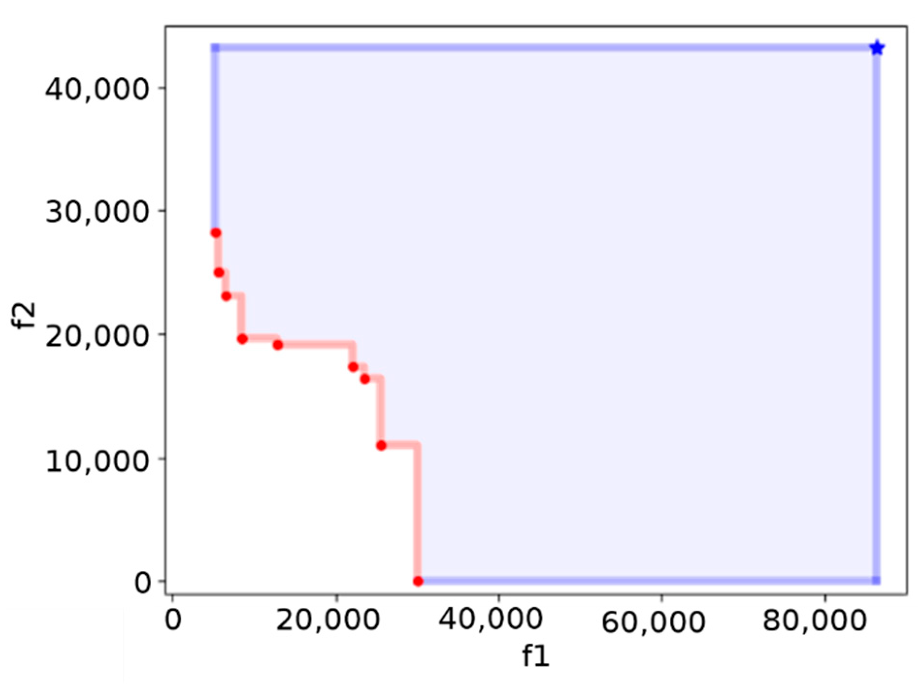
To measure the progress of the optimization a natural and widely used metric is the hypervolume indicator [17], that measures the objective space between a non-dominated set and a predefined reference vector. An example of Pareto frontier, along with the reference point to compute the hypervolume, is reported in Figure 6.
The hypervolume indicator is the golden standard in evaluating multi-objective algorithm also because it has strict Pareto compliance. However, it is computationally inefficient.
Given 2 approximations A and B of the Pareto front the C metric (Coverage) is defined by the percentage of solutions in B that are dominated by at least one solution in A.
- means that all solutions in are dominated by some solution in ;
- implies that no solution in is dominated by a solution in .
6. The Structure of MOEA/WST Algorithm
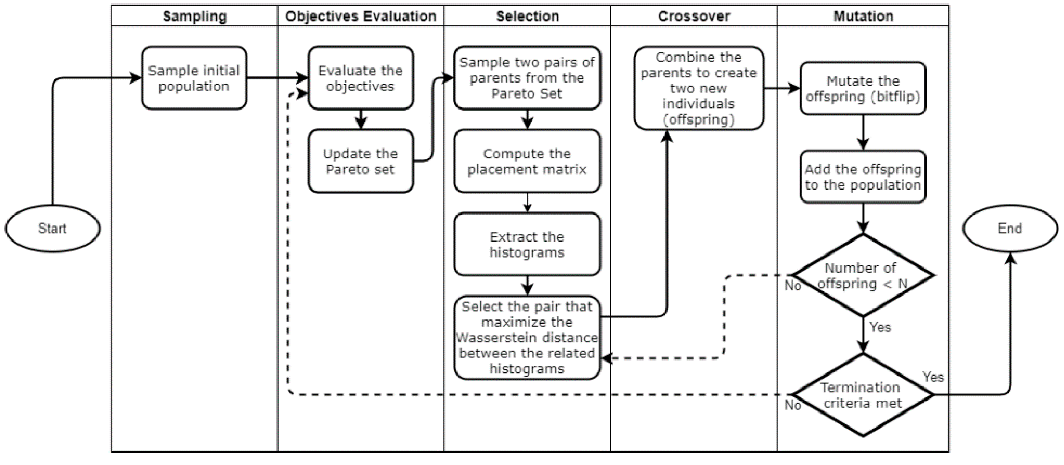
This section contains the analysis of the new algorithm proposed. It is shown how all the mathematical constructs presented in the previous sections are structured in the MOEA/WST algorithm. Section 6.1 offers a global view of the interplay of all algorithmic components which are described in the following Section 6.2, Section 6.3, Section 6.4, Section 6.5 and Section 6.6.
6.1. General Framework
Figure 7 displays the algorithmic architecture of MOEA-WST and the interaction of the different computational modules.
6.2. Chromosome Encoding
In the algorithm, each chromosome (individual) consists in a -dimensional binary array that encodes a sensor placement. Each gene represents a node in which a sensor can be placed. A gene assumes value 1 if a sensor is located in the corresponding node, 0 otherwise.
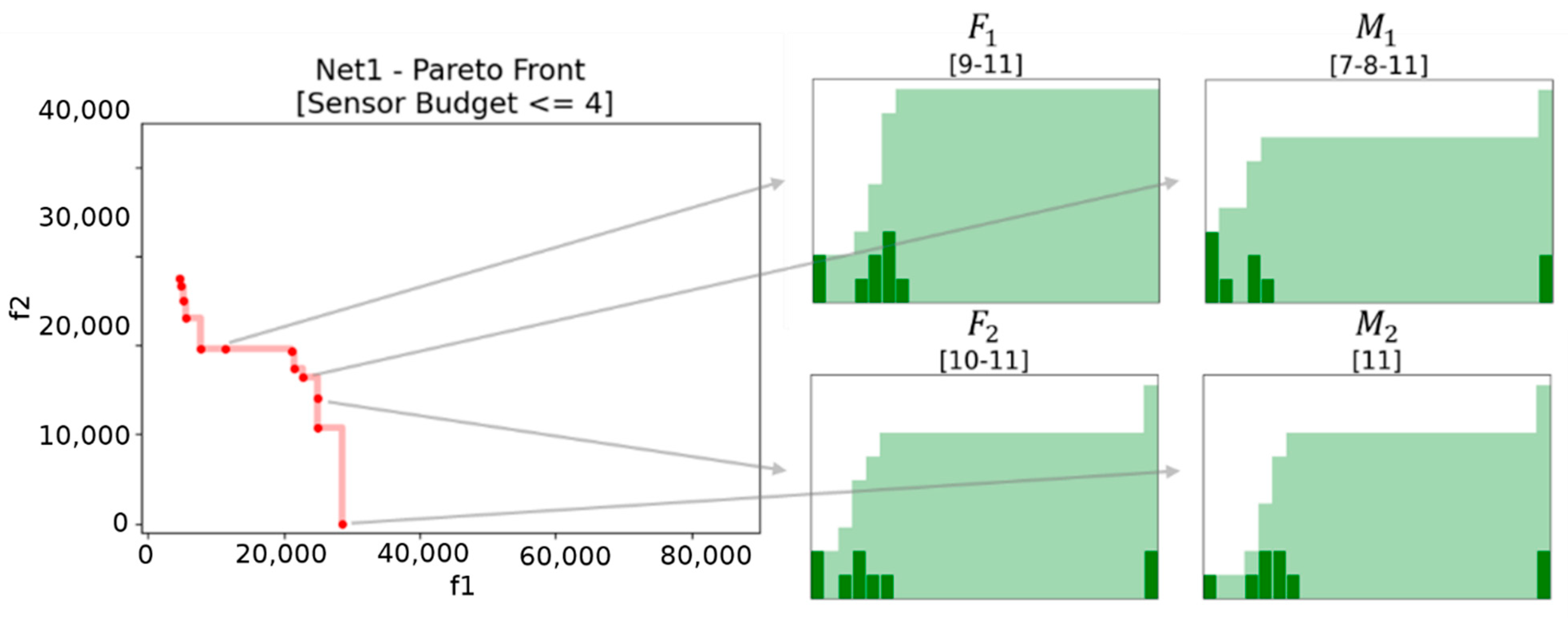
Consider the Net1 water distribution, and the individual , which means that two sensors are placed respectively in Nodes 12 and 23 as shown in Figure 8.
6.3. Initialization
The initial population has to be sampled. Our algorithm randomly samples the initial chromosomes. All the individuals in the population have to be different (sampling without replacement). This method does not guarantee to have only feasible individual. Among this population we select the non-dominated solutions (i.e., the initial approximation of the Pareto set).
6.4. Selection
In order to select the pairs of parents to be mated using the crossover operation, we have introduced a problem specific selection method that takes place into the information space (Figure 9). First, we randomly sample from the actual Pareto set two pairs of individuals and . Then we choose the pair as the parents of the new offspring, where . This favors exploration and diversification.
Any distance could be considered, for instance the Frobenius distance between two placement matrices and related to and . In this paper, we used the Wasserstein distance between the histograms corresponding to the sensor placement and .
If at least one individual of the pair of parents is not feasible (i.e., the placement contains more sensors than the budget ) the constraint violation () is considered instead. Let be a generic individual and the budget, the constraint violation is defined as follows:
Then we choose the pair of parents with .
6.5. Crossover
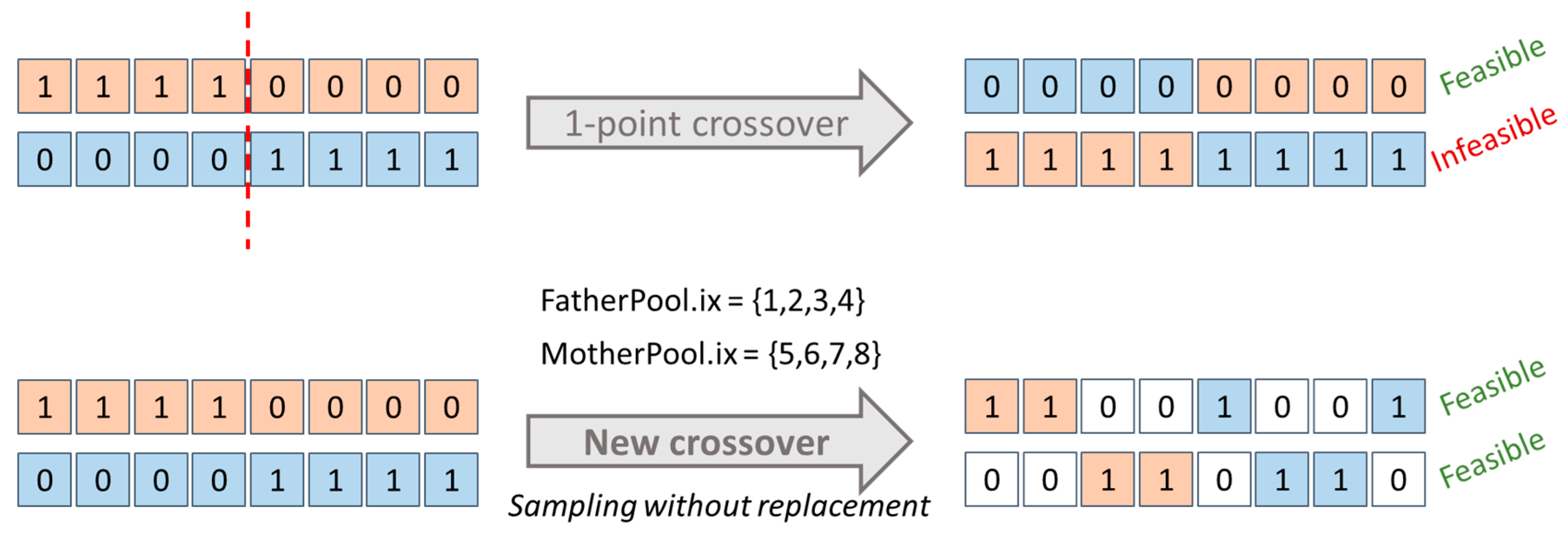
The standard crossover operators applied to sensor placement might generate unfeasible children which might induce computational inefficiency in terms of function evaluations. To avoid this in MOEA/WST, it has been introduced a problem specific crossover which generates two “feasible-by-design” children from two feasible parents
Denote with two feasible parents and with (FatherPool) and (MotherPool) the two associated sets and . To obtain two feasible children, and are initialized as . In turn, and samples an index from and from , respectively, without replacement. Therefore, the new operator rules out children with more than non-zero components.
In Figure 10, an example is shown comparing the behavior of our crossover compared to a typical 1-point crossover.
6.6. Mutation
The aim of mutation is to guarantee diversification in the population and to avoid getting trapped into local optima. We consider the bitflip mutation operator, for which a mutation probability is typically used to set the “relevance” of exploration in genetic algorithms. We have been using the bitflip mutation in Pymoo (each gene has a probability of mutation of 0.1).
7. Computational Results
7.1. Net
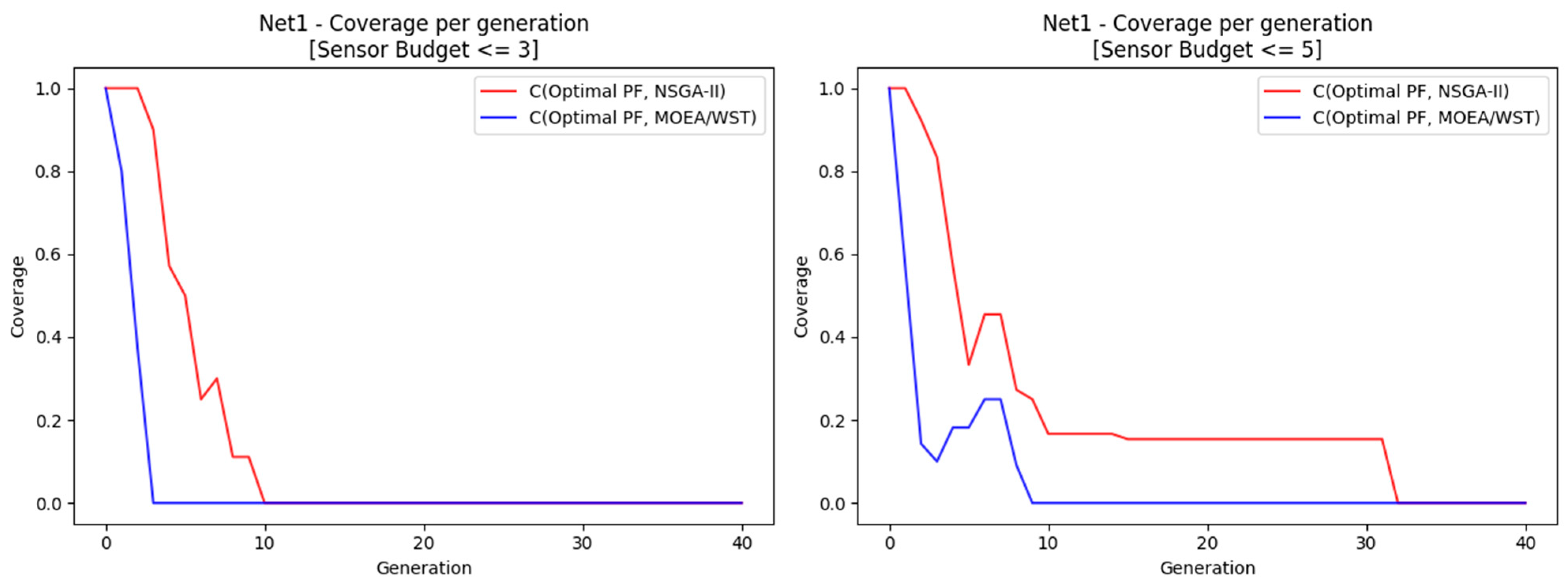
The synthetic example Net1 provided by EPANET and WNTR. The graph associated to Net1 is depicted in previous Figure 1. Net1 consists of 1 reservoir (at Location 2), 1 tank (at Location 1) and 11 junctions (nodes). The set of possible locations to deploy sensors are the 11 junctions, therefore the set is . The same junctions but and are assumed the nodes where the contaminant can be injected at, therefore .
We have considered the case that the available budget allows to have a maximum of 4 sensors in the optimal SP, that is in the constraints in (P)—valid also for the proposed bi-objective formulation. The value of has been defined according to a preliminary analysis on the single-objective problem (P): further increasing does not offer any further improvement of .
We remind that an SP is represented through a binary vector with components, with at the most components equal to 1. The search space for this example is therefore quite limited, allowing us to solve the problem via exhaustive search. More precisely, only 561 SPs are feasible according to the constraints in (P). Thus, we exactly know the Pareto set, the Pareto frontier and the associated hypervolume.
We have used Pymoo both for implementing MOEA/WST and using directly NSGA-II. In both cases, we used 100 generations and a population size of 40.
After 100 generations, NSGA-II and MOEA/WST obtained the same results in terms of hypervolume, quantile and coverage.
Figure 11 shows a significant difference in terms of the rate of convergence of the approximate Pareto to the optimal one between the two algorithms.
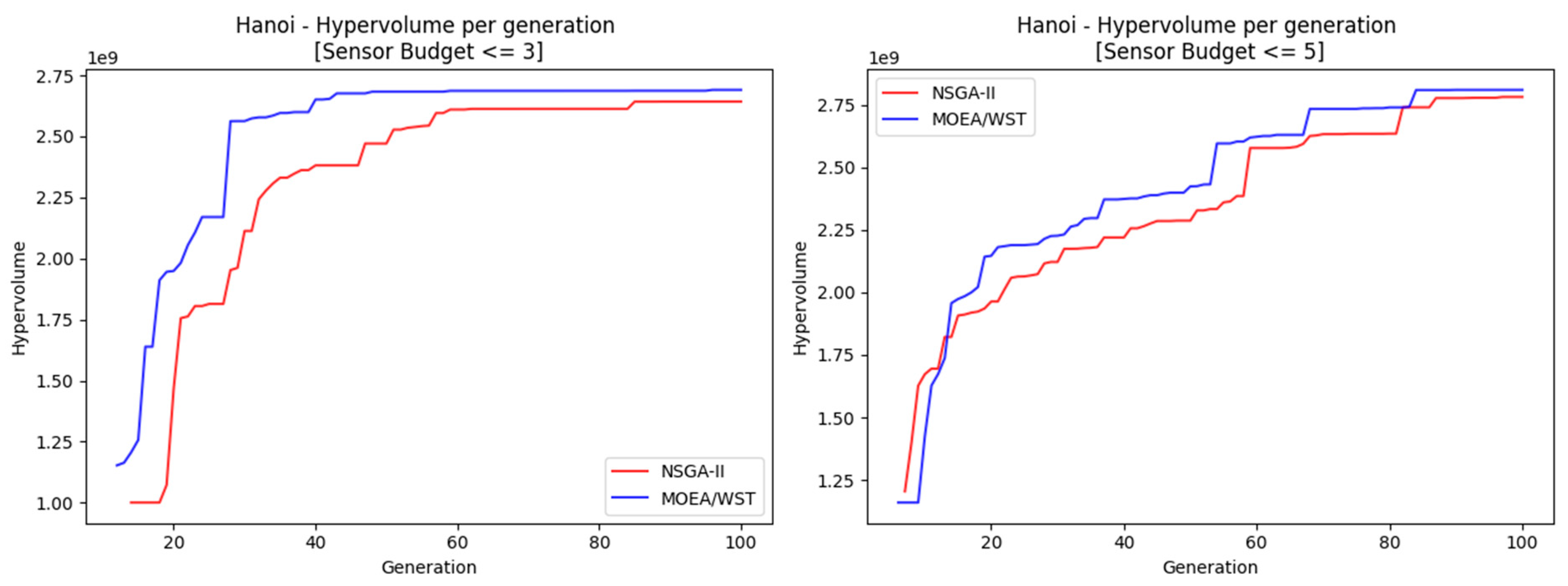
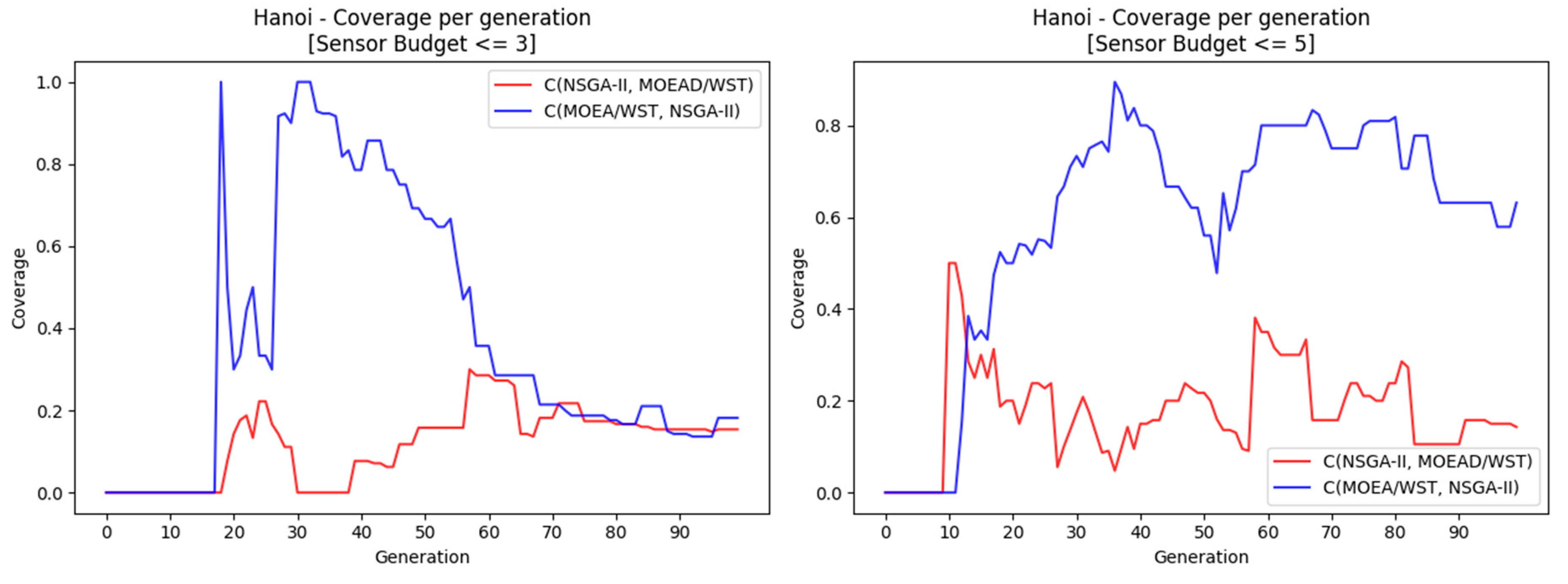
7.2. Hanoi
Hanoi is a benchmark used in the literature [18]. Figure 12 displays the graph associated to Hanoi water distribution network.
Table 1 reports the performance metrics considered for the two algorithms, NSGA-II and MOEA/WST.
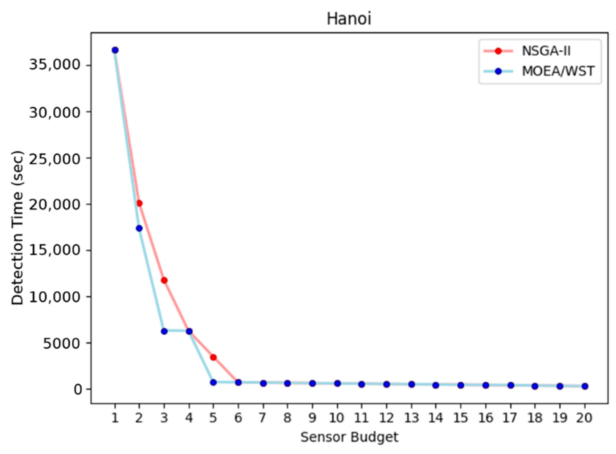
Figure 13 shows the relation between the detection time and the sensor budget.
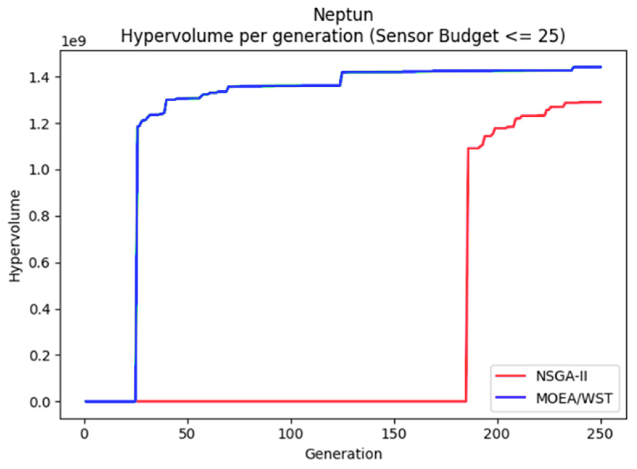
7.3. Neptun
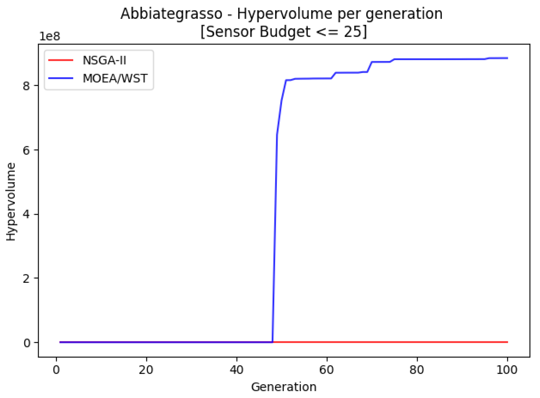
7.4. Abbiategrasso
7.5. Discussions
The computational results related to the four networks show some interesting facts.
- MOEA/WST provides a better approximation of the Pareto frontier in terms of hypervolume; moreover, it shows that the gain is significantly larger for low generation counts and as the size of the network increases.
- MOEA/WST offers a better coverage than NSGA-II. The gain is more significant in the range (knee point).
The computational results confirm that MOEA/WST is a promising solution for computationally expensive simulation-optimization multi objective black box optimization problems.
8. Conclusions
The main result of this paper is the proposal of a new evolutionary algorithms MOEA/WST for optimal sensor placement in water distribution networks. This algorithm has a more general application domain for intrusion detection problems, where the goal is to monitor the spread of “effects” triggered by “events” like, for instance detection of fake news in Web blogs.
The algorithm has been derived in the context of a sensor placement problem in a WDN as a MOP over a set of different simulated contamination events.
An important element in the algorithm is a data structure that associates to each sensor placement the dynamic representation of the contaminant concentration detected.
Exploiting this representation sensor placements, i.e., individuals in the evolutionary framework, are mapped into an information space where they can be represented as matrices or histograms. In MOEA/WST the histogram representation has been used along the Wasserstein distance.
The Wasserstein distance has been shown to be very efficient to capture the interplay of placements and to model the dependence of informational utility of placing a sensor in a location on the presence of pre-existing sensors.
In particular, the selection operator enabled by the Wasserstein distance allows a more effective diversification and exploration among candidate solutions.
A problem specific crossover operator has been also introduced which generates out of two feasible parents two “feasible-by-design” children.
The computational efficiency of the new algorithms is confirmed by the lower number of generations required for a good quality approximation of the Pareto set.
The new algorithm has been tested on two benchmark and two real-world water distribution networks yielding an improvement over a standard algorithm in terms of hypervolume and coverage, in particular at low generation counts.
This result makes MOEA/WST a potentially good candidate for a wide class of problems of computationally expensive black-box functions over combinatorial structures.
Author Contributions
All authors contributed equally to the paper. All authors have read and agreed to the published version of the manuscript.
Funding
This study has been partially supported by the Italian project “PERFORM-WATER 2030”—Programma POR (Programma Operativo Regionale) FESR (Fondo Europeo di Sviluppo Regionale) 2014–2020, innovation call “Accordi per la Ricerca e l’Innovazione” (“Agreements for Research and Innovation”) of Regione Lombardia, (DGR N. 5245/2016—AZIONE I.1.B.1.3—ASSE I POR FESR 2014–2020)—CUP E46D17000120009. This study has been also supported by the national project “ENERGIDRICA” MIUR ARS01_00625.
Institutional Review Board Statement
Not applicable.
Informed Consent Statement
Not applicable.
Data Availability Statement
The data related to the network Net1 and Hanoi are available in the literature. The data of Neptun and Abbiategrasso are available from the authors on demand.
Acknowledgments
FA acknowledges the “contribution” of his son Davide whose early fascination with the “life of a droplet” might have kindled the father’s enduring interest in all things water. We greatly acknowledge the DEMS Data Science Lab for supporting this work by providing computational resources (DEMS—Department of Economics, Management and Statistics).
Conflicts of Interest
The authors declare no conflict of interest.
Abbreviations
The following table contains the list of symbols.
| Graph underlying the water distribution network. | |
| Set of nodes . | |
| Set of edges . | |
| Set of nodes where sensors can be located. | |
| Binary vector with the sensor placement is given by the non-zero components of s. | |
| Set of nodes where contaminants can be introduced in the network. | |
| Contamination event associated to a node. | |
| Contaminant detection threshold. | |
| “Impact” of the event when detected by a sensor in . | |
| if and is the first sensor detecting the contaminant injected at Node ; otherwise. | |
| The probability for the contaminant to enter the network at Node | |
| Max number of sensors available. | |
| is the minimum detection time among the sensors in placement of event . | |
| is the sensor matrix for a sensor deployed at Node . | |
| The concentration of the contaminant in Node for the event at the simulation step . | |
| The simulation step . | |
| . | |
| Number of time intervals. | |
| Length of a time intervals Δti = ti − ti−1. | |
| is the placement matrix. | |
| Maximal contaminant concentration detected by sensors in placement at simulation step for the event . | |
| The placement histogram. | |
| Set of feasible sensor placements. | |
| The generic histogram function. | |
| Number of contamination events for which detection time happens in . | |
| The set of all joint distributions . | |
| A joint distribution . | |
| The computational process . | |
| A generic object in the information space. | |
| A generic distance. | |
| The Wasserstein distance between two probability distributions . | |
| Detection time generated by a sensor placement . | |
| Standard deviation of . | |
| Image of sensor placement s in the objective space . | |
| Coverage ratio of two approximations A and B of the Pareto front. |
References
- Candelieri, A.; Ponti, A.; Archetti, F. Risk Aware Optimization of Water Sensor Placement. arXiv 2021, arXiv:2103.04862. [Google Scholar]
- Weickgenannt, M.; Kapelan, Z.; Blokker, M.; Savic, D.A. Risk-Based Sensor Placement for Contaminant Detection in Water Distribution Systems. J. Water Resour. Plan. Manag. 2010, 136, 629–636. [Google Scholar] [CrossRef]
- Aral, M.M.; Guan, J.; Maslia, M.L. A Multi-Objective Optimization Algorithm for Sensor Placement in Water Distribution Systems. In Proceedings of the World Environmental and Water Resources Congress 2008, Ahupua’A, Honolulu, HI, USA, 12–16 May 2008; pp. 1–11. [Google Scholar]
- Ostfeld, A.; Uber, J.G.; Salomons, E.; Berry, J.W.; Hart, W.E.; Phillips, C.A.; Watson, J.-P.; Dorini, G.; Jonkergouw, P.; Kapelan, Z. The Battle of the Water Sensor Networks (BWSN): A Design Challenge for Engineers and Algorithms. J. Water Resour. Plan. Manag. 2008, 134, 556–568. [Google Scholar] [CrossRef] [Green Version]
- Margarida, D.; Antunes, C.H. Multi-Objective Optimization of Sensor Placement to Detect Contamination in Water Distribution Networks. In Proceedings of the Companion Publication of the 2015 Annual Conference on Genetic and Evolutionary Computation, Madrid, Spain, 11–15 July 2015; pp. 1423–1424. [Google Scholar]
- Naserizade, S.S.; Nikoo, M.R.; Montaseri, H. A Risk-Based Multi-Objective Model for Optimal Placement of Sensors in Water Distribution System. J. Hydrol. 2018, 557, 147–159. [Google Scholar] [CrossRef]
- Berry, J.; Hart, W.E.; Phillips, C.A.; Uber, J.G.; Watson, J.-P. Sensor Placement in Municipal Water Networks with Temporal Integer Programming Models. J. Water Resour. Plan. Manag. 2006, 132, 218–224. [Google Scholar] [CrossRef] [Green Version]
- Zhao, Y.; Schwartz, R.; Salomons, E.; Ostfeld, A.; Poor, H.V. New Formulation and Optimization Methods for Water Sensor Placement. Environ. Model. Softw. 2016, 76, 128–136. [Google Scholar] [CrossRef]
- Klise, K.A.; Murray, R.; Haxton, T. An Overview of the Water Network Tool for Resilience (WNTR); Sandia National Lab.(SNL-NM): Albuquerque, NM, USA, 2018. [Google Scholar]
- Monge, G. Mémoire Sur La Théorie Des Déblais et Des Remblais; Histoire De L’académie des Science de Paris; De l’Imprimerie Royale: Paris, France, 1781. [Google Scholar]
- Kantorovitch, L. On the Translocation of Masses. Manag. Sci. 1958, 5, 1–4. [Google Scholar] [CrossRef]
- Weng, L. From Gan to Wgan. arXiv 2019, arXiv:1904.08994. [Google Scholar]
- Villani, C. Optimal Transport: Old and New; Springer Science & Business Media: Berlin/Heidelberg, Germany, 2008; Volume 338. [Google Scholar]
- Peyré, G.; Cuturi, M. Computational Optimal Transport: With Applications to Data Science. Found. Trends Mach. Learn. 2019, 11, 355–607. [Google Scholar] [CrossRef]
- Öcal, K.; Grima, R.; Sanguinetti, G. Parameter Estimation for Biochemical Reaction Networks Using Wasserstein Distances. J. Phys. A Math. Theor. 2019, 53, 034002. [Google Scholar] [CrossRef] [Green Version]
- Arjovsky, M.; Chintala, S.; Bottou, L. Wasserstein Generative Adversarial Networks. In Proceedings of the International Conference on Machine Learning; PMLR: Sydney, Australia, 2017; pp. 214–223. [Google Scholar]
- Zitzler, E.; Künzli, S. Indicator-Based Selection in Multiobjective Search. In Proceedings of the International Conference on Parallel Problem Solving from Nature; Springer: Berlin/Heidelberg, Germany, 2004; pp. 832–842. [Google Scholar]
- Vasan, A.; Simonovic, S.P. Optimization of Water Distribution Network Design Using Differential Evolution. J. Water Resour. Plan. Manag. 2010, 136, 279–287. [Google Scholar] [CrossRef]
- Candelieri, A.; Soldi, D.; Archetti, F. Cost-Effective Sensors Placement and Leak Localization–the Neptun Pilot of the ICeWater Project. J. Water Supply Res. Technol. AQUA 2015, 64, 567–582. [Google Scholar] [CrossRef]
- Fantozzi, M.; Popescu, I.; Farnham, T.; Archetti, F.; Mogre, P.; Tsouchnika, E.; Chiesa, C.; Tsertou, A.; Gama, M.C.; Bimpas, M. ICT for Efficient Water Resources Management: The ICeWater Energy Management and Control Approach. Procedia Eng. 2014, 70, 633–640. [Google Scholar] [CrossRef]
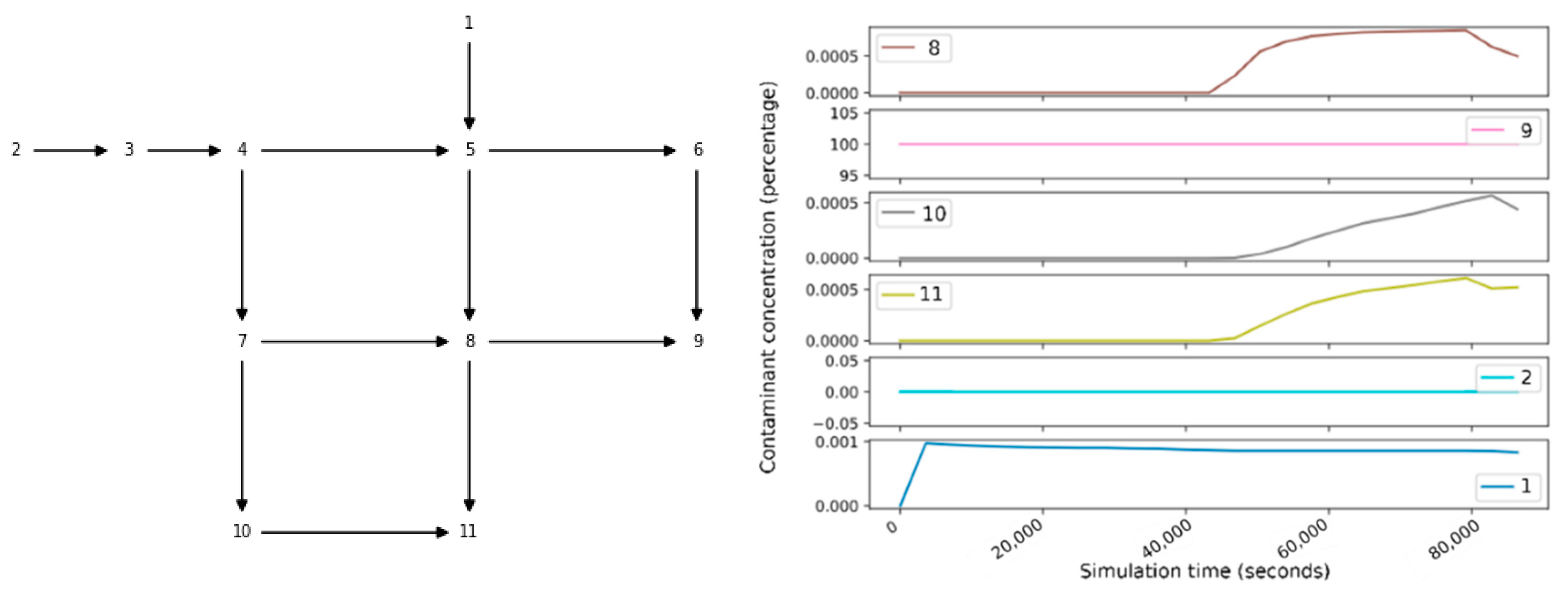
Figure 1.
A schematic representation of the Net1 synthetic example (left). Concentrations of the contaminant introduced at Node 9 for Nodes 1, 2, 8, 9, 10, and 11 (right).
Figure 1.
A schematic representation of the Net1 synthetic example (left). Concentrations of the contaminant introduced at Node 9 for Nodes 1, 2, 8, 9, 10, and 11 (right).

Figure 2.
Sensor matrices and for sensors deployed respectively at locations, i.e., Node 9 (left) and Node 11 (right).
Figure 2.
Sensor matrices and for sensors deployed respectively at locations, i.e., Node 9 (left) and Node 11 (right).

Figure 3.
Sensor placement matrix for a sensor placement consisting of two sensors deployed at Locations 9 and 11.
Figure 3.
Sensor placement matrix for a sensor placement consisting of two sensors deployed at Locations 9 and 11.

Figure 4.
The histogram of a sensor placement with p = 4 (|A| = 9).

Figure 5.
Search space, information space and objectives.

Figure 6.
An example of Pareto frontier, with the associated hypervolume, for two minimization objectives ( is the detection time and is its standard deviation).
Figure 6.
An example of Pareto frontier, with the associated hypervolume, for two minimization objectives ( is the detection time and is its standard deviation).

Figure 7.
The general structure of MOEA/WST.

Figure 8.
A sensor placement example considering Net1.

Figure 9.
Two pairs of individuals are randomly sampled from the actual Pareto front. In this example, the pairs is choosen because .
Figure 9.
Two pairs of individuals are randomly sampled from the actual Pareto front. In this example, the pairs is choosen because .

Figure 10.
A schematic representation of the new crossover operator.

Figure 11.
Coverage between the optimal Pareto frontier and the approximate one.

Figure 12.
A schematic representation of the Hanoi water distribution network.

Figure 13.
Detection time over the budget.

Figure 14.
Hypervolume per generation.

Figure 15.
Coverage per generation.

Figure 16.
Hypervolume per generation.

Figure 17.
Hypervolume per generation.


Table 1.
Metric (Hanoi—50 generation).
| Metric | Hypervolume (×106) | Coverage | ||
|---|---|---|---|---|
| Algorithm | NSGA-II | MOEA/WST | C(NSGA-II, MOEA/WST) | C(MOEA/WST, NSGA-II) |
| Budget 2 | 2278.42 | 2458.66 | 0.33 | 0.50 |
| Budget 3 | 2470.80 | 2682.93 | 0.16 | 0.69 |
| Budget 4 | 2619.83 | 2643.73 | 0.31 | 0.58 |
| Budget 5 | 2287.12 | 2424.12 | 0.22 | 0.62 |
| Budget 10 | 2427.64 | 2531.23 | 0.28 | 0.64 |
| Budget 15 | 2569.29 | 2511.22 | 0.725 | 0.125 |
Publisher’s Note: MDPI stays neutral with regard to jurisdictional claims in published maps and institutional affiliations. |
© 2021 by the authors. Licensee MDPI, Basel, Switzerland. This article is an open access article distributed under the terms and conditions of the Creative Commons Attribution (CC BY) license (https://creativecommons.org/licenses/by/4.0/).
Share and Cite
MDPI and ACS Style
Ponti, A.; Candelieri, A.; Archetti, F. A New Evolutionary Approach to Optimal Sensor Placement in Water Distribution Networks. Water 2021, 13, 1625. https://doi.org/10.3390/w13121625
AMA Style
Ponti A, Candelieri A, Archetti F. A New Evolutionary Approach to Optimal Sensor Placement in Water Distribution Networks. Water. 2021; 13(12):1625. https://doi.org/10.3390/w13121625
Chicago/Turabian StylePonti, Andrea, Antonio Candelieri, and Francesco Archetti. 2021. "A New Evolutionary Approach to Optimal Sensor Placement in Water Distribution Networks" Water 13, no. 12: 1625. https://doi.org/10.3390/w13121625
Note that from the first issue of 2016, this journal uses article numbers instead of page numbers. See further details here.