Peculiarities of Hydrodynamics of Small Surface Water Bodies in Zones of Active Technogenesis (on the Example of the Verkhne-Zyryansk Reservoir, Russia)

Abstract

As a rule, large modern industrial complexes are significant water users. This raises the problem of providing them with reliable and sustainable water supply systems. To solve this problem, relatively small, special reservoirs for technical water supply are often created. When creating them, it is a priori assumed that their water masses will be comparatively homogeneous over the aquatorium and throughout the depths, and so, therefore, that their flushing can be successfully used to prevent a possible accumulation of pollutants. The experience of operating such reservoirs in the Verkhnekamsky potassium and magnesium salt development zone in Ural, Russia, has shown that, due to intense diffuse pollution, the reservoirs are characterized by significant vertical non-uniformity, fundamentally altering the hydrodynamics of these water bodies. Based on a series of research, including field observations and computational experiments, the present paper reveals that the vertical non-uniformity of water masses plays a key role in ensuring the sustainability of technical water supply.

1. Introduction

River regulation as a means of water resource management is a universally recognized practice for the optimum control of water use from natural and artificial reservoirs. Reservoir discharge is one of the most important characteristics of river regulation, which must be considered when meeting energy demands, maintaining water levels during floods, and controlling water quality [1,2]. Another equally important aspect of water resource management is density currents, which take place in the river-reservoir system due to the density and non-uniformity of water masses in these reservoirs caused by temperature and concentration inhomogeneities. Over the past decades, many experimental and numerical studies were carried out to gain a better understanding of density currents (see, for example [3,4,5,6,7,8]). Density currents were also studied in laboratory experiments [9,10,11].

Model studies of density flows were carried out for inclined channels with a rectangular cross-section. The analytical models were elaborated based on various simplifying assumptions, and subsequently verified using laboratory data [12,13,14]. The formation of density currents in watercourses of real geometry is the problem that is extensively studied at the present time [15,16,17,18,19,20,21]. For example, works [17] and [18] investigate the formation of density currents by regulating the discharge of water. In [17], a combined hydrothermodynamic model was used and analytical solutions were developed for the distribution of water temperature in the river. The obtained solutions provide deeper insight into the physical properties associated with the propagation of both hydrodynamic and thermal peak waves in the downstream of the receiving river. It was shown that the dynamics of hydrodynamic and thermal waves is rather complex: a thermal wave always propagates more slowly than a hydrodynamic wave, and their decay also occurs slowly.

However, paper [17] does not consider the formation of density currents in the receiving river. Such a study was carried out in [18] within the framework of a three-dimensional model of a system of reservoirs extending for 124 km from the Lewis Smith Dam to the Bankhead Lock and Dam, Alabama. Consideration was given to normal water discharge (2.83 m³/s) and maximum water discharge (~140 m³/s) from the upper reservoir. The research took heat exchange with the atmosphere in the river-reservoir system into account. It was shown that at normal water discharge, the movement in the surface and bottom layers was observed both upstream and downstream, and the bottom temperature was, on average, 4.8 °C higher than the temperature of the discharged water. The momentum generated by the maximum discharge of water displaces the lower density currents downstream, leading to a decrease in temperature near the bottom. In the case when several rivers enter the reservoir, the formation of density currents is the result of temperature differences and the chemical composition of the incoming water [19]. At the confluence, colder and warmer flows generate lower and surface floating outlet streams, respectively. The appearance of stagnant zones with long residence times leads to algal bloom and hypoxia. The mechanism of the formation of a large-scale salinity eddy at the confluence of two rivers with different salinities was described in detail in [20]. The influence of the consequences of a fire on the physicochemical properties of water in a reservoir used for water supply was considered in [22]. Here also, the spatial and temporal characteristics of sediments, the hydrodynamics of the reservoir, and the erodibility of the catchment area were investigated.

The study of density effects from the viewpoint of water quality formation in reservoirs and lakes is of considerable interest. These questions were considered in [23,24,25,26].

To ensure effective water quality management in dam reservoirs, it is necessary to understand the transport and mixing of pollutants. The main mechanisms affecting mass transport are highly dependent on the type of reservoir and operating conditions. For example, for a reservoir operating as a riverbed in which, due to the inflow discharge, there is a small change in water level [27], the physical and chemical properties of the river inflow are the main determinants of the aquatic environment in the reservoir [28,29]. The second type of reservoir is created to meet the needs for technical water. The stability of technical water supply to large industrial enterprises is one of the most important factors responsible for the reliability of their performance. This problem is especially acute for enterprises located in zones of active technogenesis, where the dominant factor in the formation of water pollution is the presence of non-declared dispersed (so-called diffuse), sources of pollution. The reservoirs created on this territory for the purpose of technical water supply have a number of peculiarities that must be considered in their designing.

Traditionally, it is believed that the distribution of pollutants is fairly uniform over the depth of water bodies. This viewpoint is taken as a prime consideration when organizing the system of impact for the monitoring of water bodies, when it is considered acceptable to take water samples only from the surface and characterize the discharged wastewater by neutral buoyancy. The above statement is true for relatively shallow water bodies with intense vertical turbulent exchange, for which the density Froude numbers are Fr > 1 and, accordingly, the Richardson numbers are Ri < 1.

The density Froude number is defined as:

$$\mathrm{Fr}\mathsf{\rho }=\frac{V}{\sqrt{\left(\frac{\Delta \mathsf{\rho }}{\mathsf{\rho }}\right)\times H\times g}}$$

The Richardson number is defined as:

$$\mathrm{Ri}= \frac{\frac{\partial \mathsf{\rho }}{\partial z}}{\mathsf{\rho }\times g{\left(\frac{\partial V}{\partial z}\right)}^2}~\frac{\left(\frac{\Delta \mathsf{\rho }}{\mathsf{\rho }}\right)\times H\times g}{V^2}$$

where V is the characteristic flow velocity, $\frac{\Delta \mathsf{\rho }}{\mathsf{\rho }}$ is the relative difference in water density, H is the flow depth, and g is the acceleration of gravity. In the area of water intake structures, the Fr is ~0.08–0.2, while the Ri is ~25–156.3.

However, in water bodies with slow water exchange, primarily in reservoirs located in the zones of active technogenesis, these basic provisions are not fulfilled and lead to the formation of significant vertical density heterogeneities, which fundamentally change the conditions of water use. At the same time, in traditional assessments of the sustainability of the water use systems, these features are often ignored.

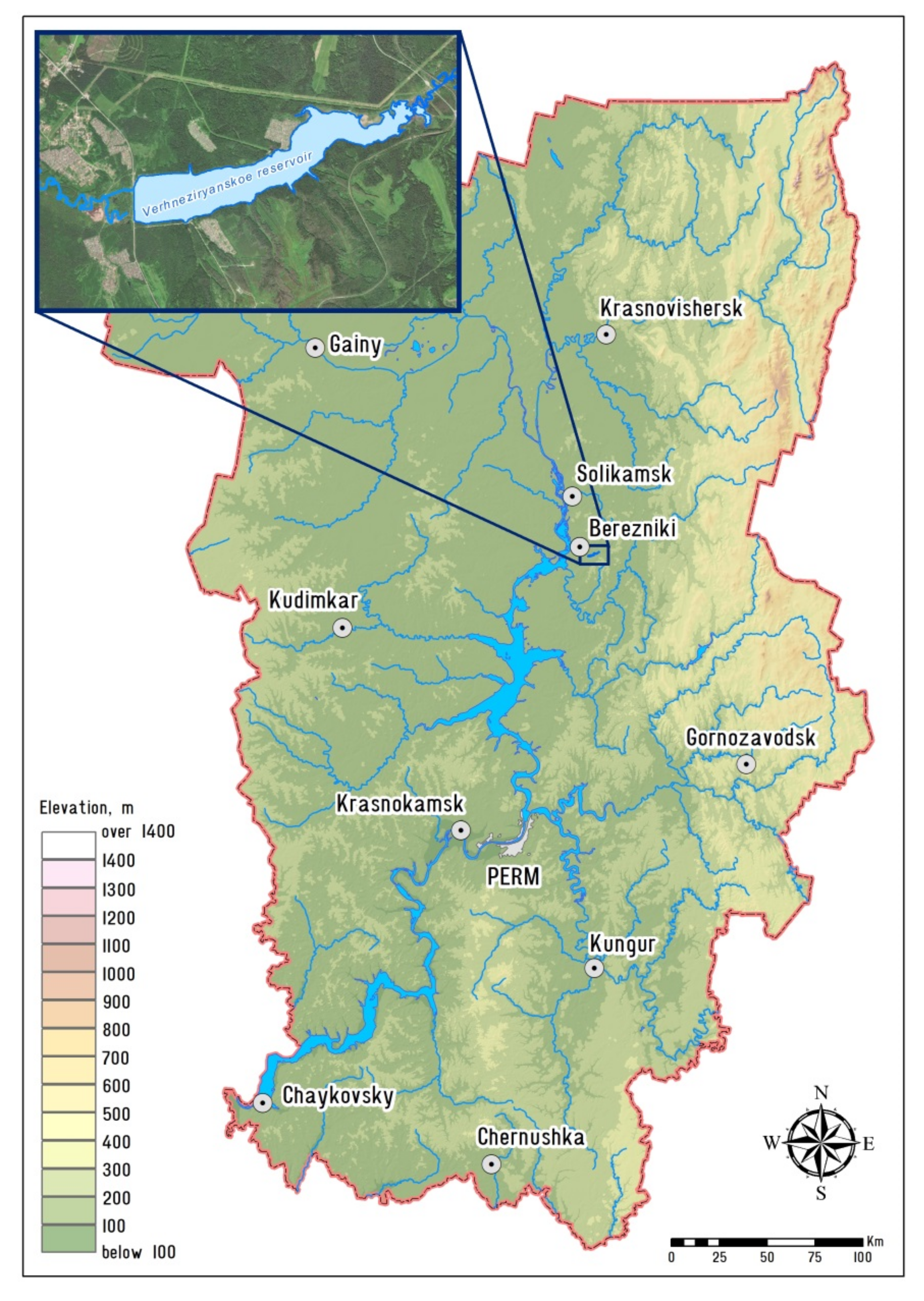
In the present paper, the above stated problem is investigated using, as an example, an industrial BKPRU-4 unit, which was designed to supply technical water from the Verkhne-Zyryansk reservoir (Figure 1). A specific feature of this water body is its location in the zone of active technogenesis, where filtration discharges are active [30]. As is evident from a series of field studies, this reservoir is characterized by significant vertical non-uniformity of water masses, which has a strong effect on the sustainability of water use.

To clarify the reasons for significant intra-annual oscillations of salinity in the water taken from the water intake, a bathymetric survey of the reservoir and a detailed conductometric survey of the reservoir water area were carried out. The specific electrical conductivity profile was constructed and the corresponding hydrodynamic models were developed to assess the stability of the vertical non-uniformity of the water masses under various hydrological regimes of reservoir operation.

2. Materials and Methods of Field Measurements

The Verkhne-Zyryansk reservoir is located in the valley of the Zyryanka River. The Zyryanka River is a left-bank tributary of the Kama River, the confluence of which is situated at a distance of 889 km from the mouth. The Zyryanka River is formed as a result of the confluence of the Izver and Legchim rivers. The total catchment area of the Zyryanka River is 365 km², the length of the river is 53.0 km (with the Izver River), and the average slope of the river is 2.20%. The number of watercourses in the catchment is 116, with their total length equaling 243.7 km.

The river in the middle and lower reaches is blocked by dams, which form the Verkhne-Zyryansk and Nizhne-Zyryansk (Seminsky pond) reservoirs. In the area between the reservoirs, there are 5 significant tributaries, the largest of which is the Bygel River. The gates of the dams are located at distances of 11.0 km and 1.0 km from the mouth of the Zyryanka River. The cascade of reservoirs on the Zyryanka River is considered a single water management system, providing seasonal flow regulation in the catchment area of this river. The Verkhne-Zyryansk reservoir is located 3.5 km south-east of Berezniki. It was built and put into operation in 1969. The soils of these reservoir catchment areas are predominantly composed of clayey and heavy loamy soil. Depressions contain peats and peat-gley soils. Quaternary and Upper Permian deposits contribute much to the formation of the geological structure of the reservoir bed.

The vegetation is represented mainly by mid-taiga forests with a predominance of conifer forests, sometimes in combination with an admixture of fir, aspen, and birch forests, and sphagnum bogs or pine forests on the sands. On poor soils, the admixture of broad-leaved species is noticeably reduced. According to the updated data, about 90% of the drainage area of the Verkhne-Zyryansk reservoir is covered by forests.

The system of the hydrotechnical structures of the Verkhne-Zyryansk reservoir includes: a reservoir with a dam, a spillway, and a technical water supply unit. The morphometric characteristics of the Verkhne-Zyryansk reservoir, which have been specified in [31], are given below:

• Forced level 0.1% is 124.3 m abs;
• Normal head water level is 124.0 m abs;
• Lowest water level is 121.0 m abs;
• Full volume is 13 million m³;
• Useful volume is 10 million m³;
• The area of the surface at the normal head water level is 4.2 km²;
• The level of the highest drawdown level is 123.0 m, as per the rules for the safe operation of the Verkhne-Zyryansk reservoir;
• The length of the reservoir at the normal head water level is 7 km;
• The average width at normal head water level is 0.6 km;
• The average depth at normal head water level is 3.1 m.

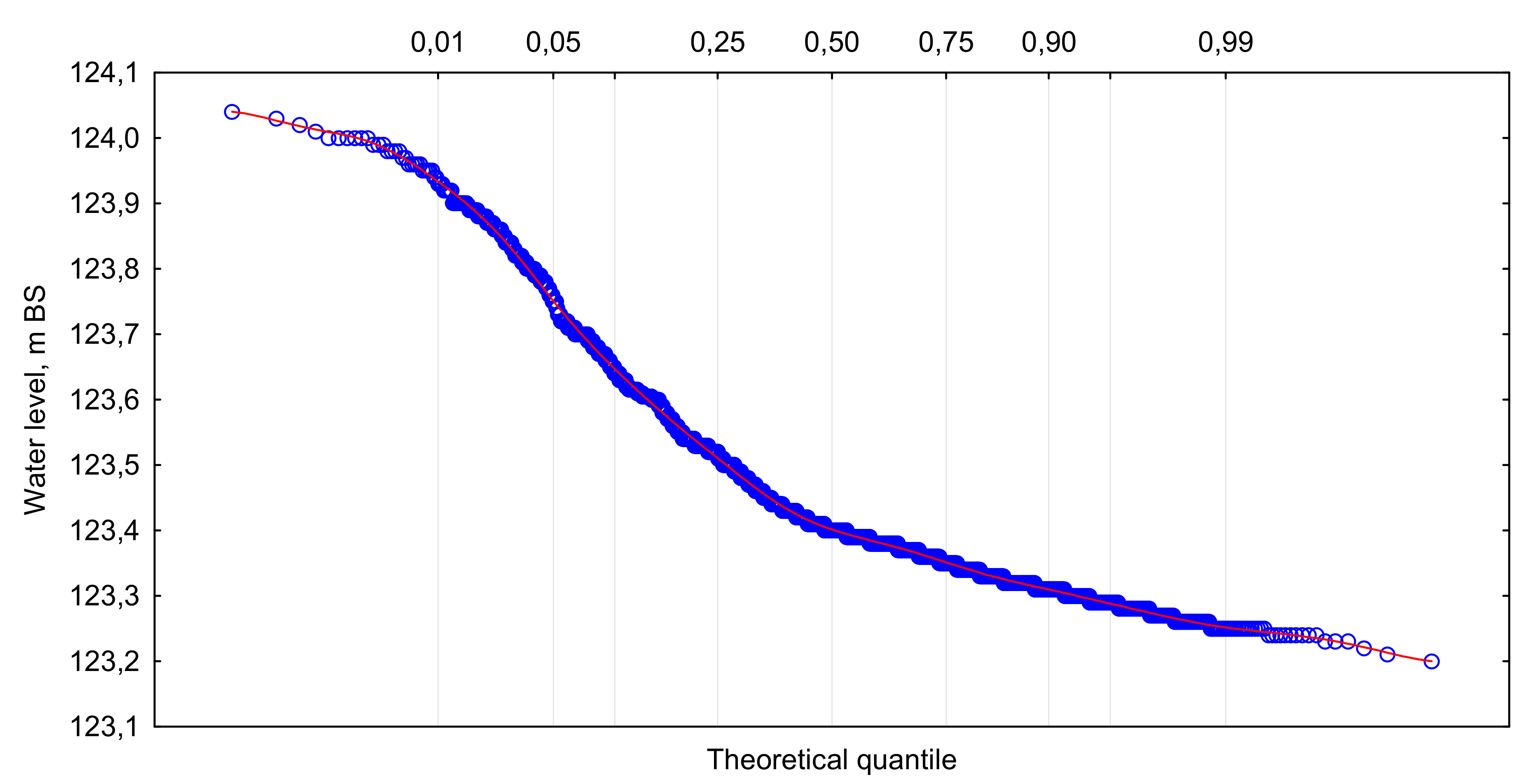
The water level in the upper pool of the Verkhne-Zyryansk reservoir is very stable and, on average, it is kept at about 123.4 m abs, which is 0.6 m below the normal head water level and, accordingly, 0.9 m below the forced level 0.1% (Figure 2).

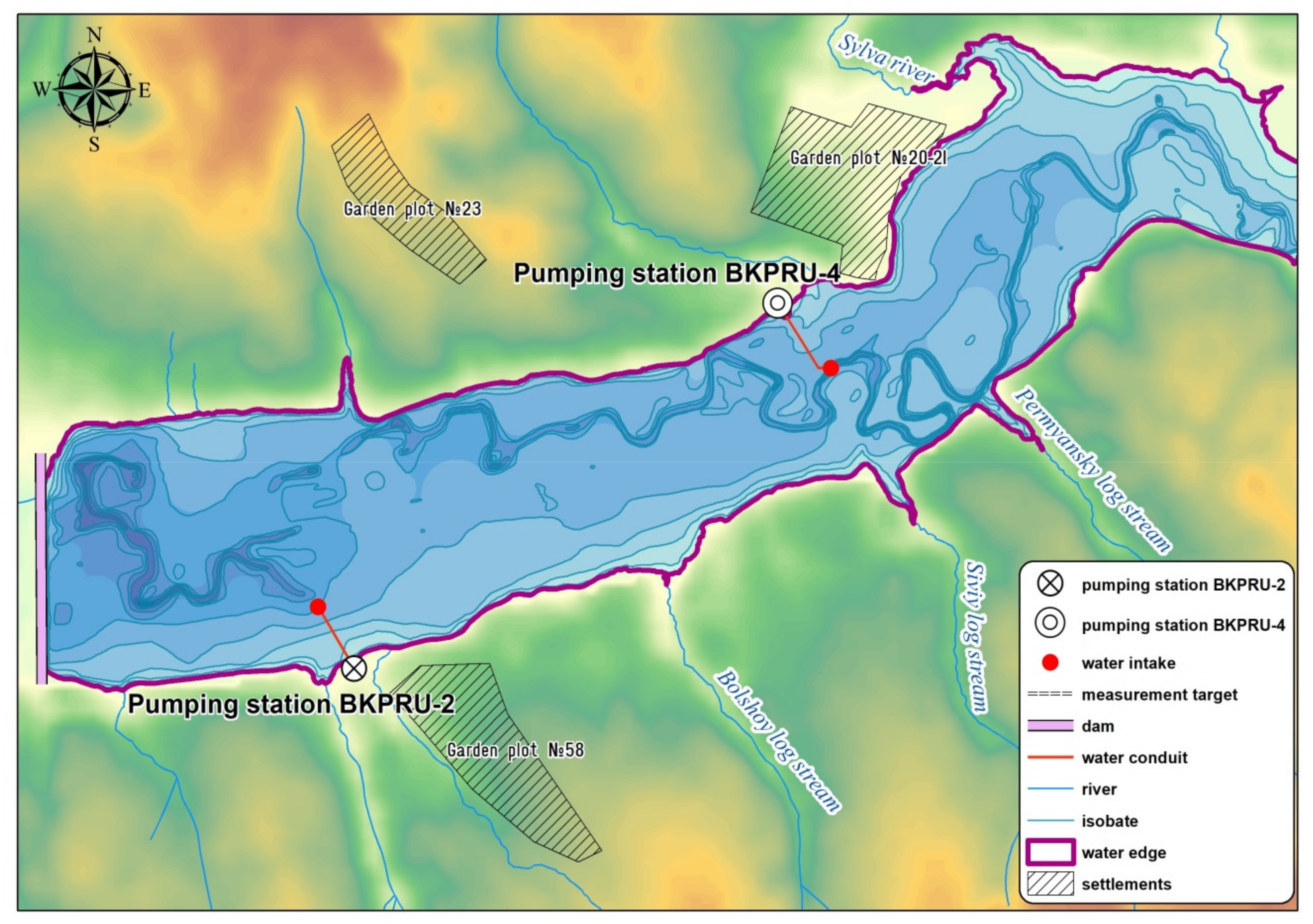
This reservoir is the main source of the industrial water supply for the BKPRU-2 and BKPRU-4 units (Bereznikovskoye Potash Production ore management) of PJSC Uralkali (Figure 3), and it is also used for recreational purposes. In the last three years, there have been serious problems with ensuring the sustainability of the water supply of this enterprise due to an increase in the salinity of the withdrawn water. The difficulties are strongly aggravated by the fact that this area is characterized by significant diffuse pollution, as is shown in [31,32,33].

Due to these circumstances, a comprehensive survey of the Verkhne-Zyryansk reservoir was carried out in 2020 with the aim of determining the cause of the high salt content in the water taken from the intake heading in winter, which could limit the use of water intake for technical needs. The following ingredients are considered as a priority for the potash industry: potassium, sodium, magnesium, calcium, chlorides, sulfates, and dry residue.

A portable field conductometer ProfiLine Cond 1970, manufactured by WTW (Weilheim, Germany), was used as the main measuring device for the assessment of changes in water quality indicators throughout the depth of the water body. This conductometer is designed to measure electrical conductivity (EC) and temperature in natural and discharged waters. In addition, the EC values reduced to a given water temperature (25 °C), rather than the current EC measurements, were used in order to allow for a comparative analysis of the measurement results in the winter and summer periods.

The use of EC values, which form a sufficiently stable qualitative composition of the main macrocomponents that determine the hydrochemical regime of the water body, is closely related to water mineralization, making it possible to conduct a more detailed survey of the water body. To control changes in the qualitative composition of the macrocomponents at each cross-section, water samples were taken from the surface and bottom horizons to determine the content of the main chemical macrocomponents. In the winter period, an off-ice study of the vertical distribution of electrical conductivity was carried out, whereas in the summer period the study was conducted with the help of a floating craft. The measurements of the electrical conductivity of water were taken vertically from the surface to the bottom horizon using the one-meter step. In zones with a sharp change in the values of electrical conductivity, exceeding 20%, the step was decreased to 0.5-0.25 m. The location of the measuring verticals was determined by means of the satellite global positioning system (GPS/GLONASS). The transverse profiles, constructed with the use of the results of the measurements, clearly demonstrate changes in the electrical conductivity over the depth and width of the reservoir. A total of 10 cross-sections were used for the analysis.

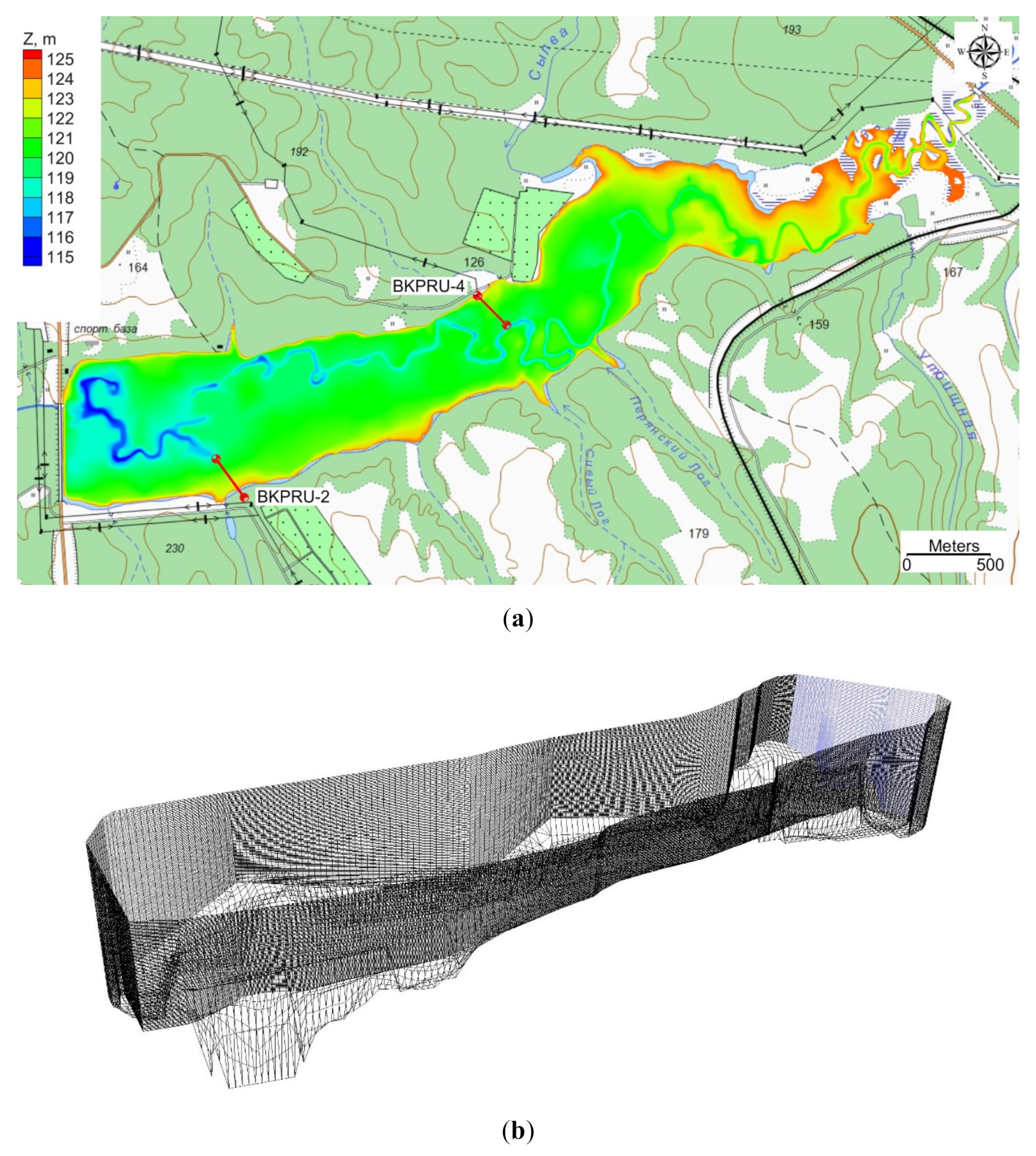
The distribution of water depths in the Verkhne-Zyryansk reservoir is shown in Figure 3. The maximum depth in the reservoir is 11 m, with the greatest depths observed along the old water course of the Zyryanka River.

A peculiarity of the BKPRU-4 water intake structure is the high inhomogeneity of the intra-annual salinity of the intake water. During the ice-free period (from May to October), the composition of the river water, on average, is typical for the formation of natural conditions of hydrocarbonate-calcium mineralization, ranging from 0.2 to 0.3 g/L. Then, from November to March there is a dramatic increase in the mineralization of the water from 0.5 to 0.6 g/L, as well as a sharp increase in the proportion of sulfates and chlorides in the salt composition. This is partly due to natural seasonal changes in the feeding of the water body. During the winter low-water period, which involves ice formation, the share of the more mineralized groundwater in the feeding of the water body grows significantly, whereas during the spring flood and summer-autumn low-water period, the water reservoirs are filled with less mineralized rain and melt waters.

Another process associated with the winter low-water period is a decrease in surface inflow into the reservoir. The main source of feeding water is groundwater, which is more mineralized. This leads to an increase in the total mineralization of the water in the reservoir. During this period, a decrease in water quality is recorded at the water intake.

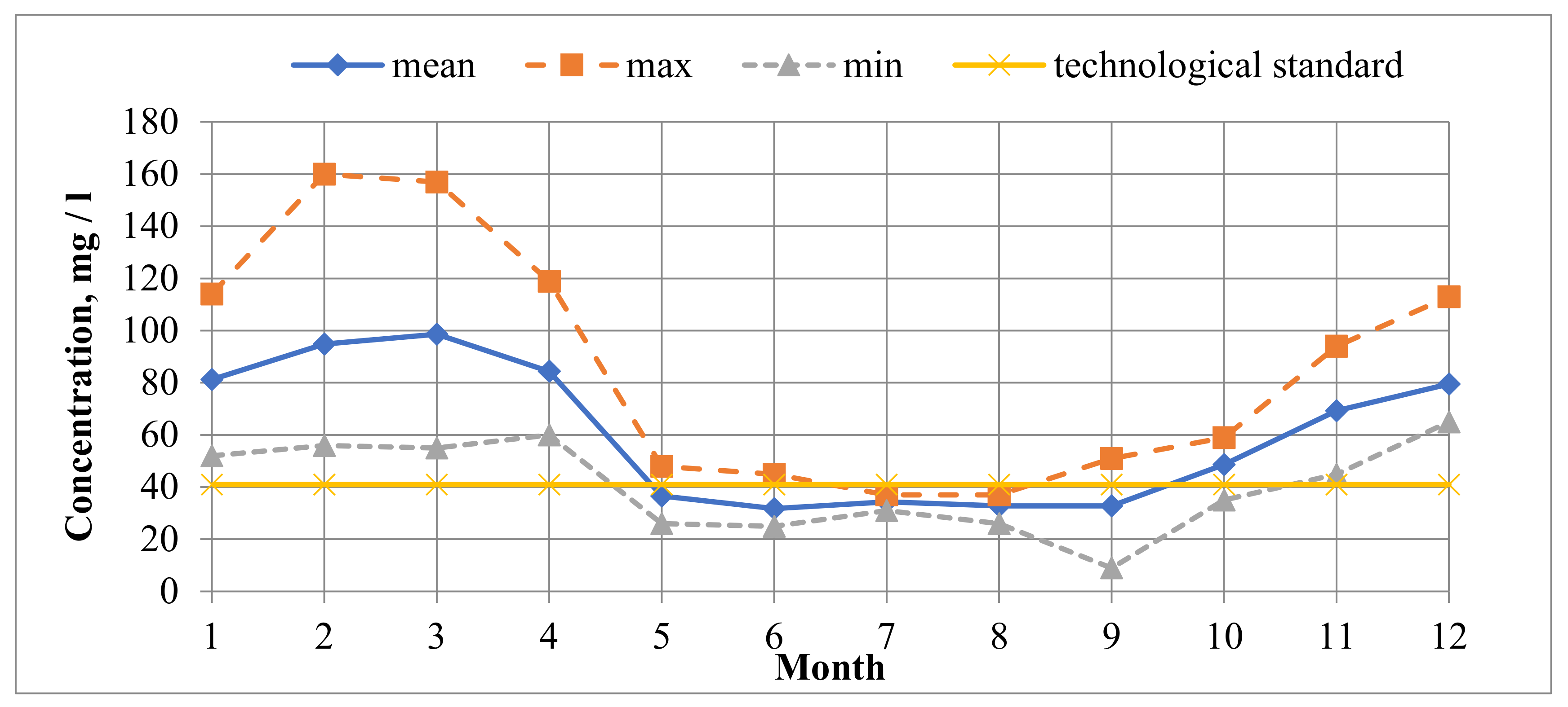
In general, it should be noted that the quality of water during the freeze-up period does not correspond to the established technological standards, mainly in terms of the content of calcium, magnesium, chlorides, and sodium (Figure 4,

Table 1. The results of the chemical analysis of water samples taken by the Mining Institute of the Ural Branch of the Russian Academy of Sciences during the winter dry season on 25 March 2020 from the Verkhne-Zyryansk reservoir.

		Water Intake BKPRU-2 (Bottom, 4.5 m)	Water Intake BKPRU-4 (Surface)	Water Intake BKPRU-4 (Horizon 4.5 m)	Water Intake BKPRU-4 (Bottom)
Chloride ions	mg/dm3	541 ± 54	14.7 ± 1.5	516 ± 52	3694 ± 369
Sulfate ions	mg/dm3	53 ± 5	44.1 ± 4.4	132 ± 13	140 ± 14
Calculated bicarbonate ion	mg/dm3	218 ± 26	168 ± 20	211 ± 25	196 ± 24
General hardness	dHG	11.26 ± 0.56	3.96 ± 0.20	13.05 ± 0.65	>50
Calcium	mg/dm3	164 ± 16	53.7 ± 5.4	191 ± 19	1091 ± 109
Magnesium	mg/dm3	43.6 ± 4.4	12.5 ± 1.3	51.5 ± 5.2	459 ± 46
Potassium	mg/dm3	16.1 ± 1.6	2.01 ± 0.28	19.5 ± 2.0	<0.5
Sodium	mg/dm3	198 ± 20	8.3 ± 1.2	169 ± 17	78.9 ± 7.9
Dry residue	mg/dm3	1212 ± 109	248 ± 22	1268 ± 114	7502 ± 375

).

It should be noted that the culverts of the Verkhne-Zyryansk reservoir, due to their design features, are capable of operating only up to the ULV mark (121 m abs). In the lower layers of the reservoir (due to the impossibility of effectively washing them), there is a gradual accumulation of various pollutants, including macrocomponents of the salt composition, which can, in turn, limit the use of the reservoir in terms of the quality of the water taken over time. This effect is confirmed by the results of observations in the area of the BKPRU-4 intake header, where a pronounced stratification, in the form of an increase in the content of the main macrocomponents of the water’s salt composition from the surface to the bottom of the reservoir, is observed both over the freeze-up and open channel periods. This phenomenon is more pronounced in winter, when the content of chlorides in the water increases by a factor of 250. The content of calcium, magnesium, and overall hardness also significantly increases. It should be noted that the concentration of sulfates and chlorides in the Zyryanka River’s upper reaches and downstream of the Verkhne-Zyryansk reservoir dam do not undergo significant changes (Table 1).

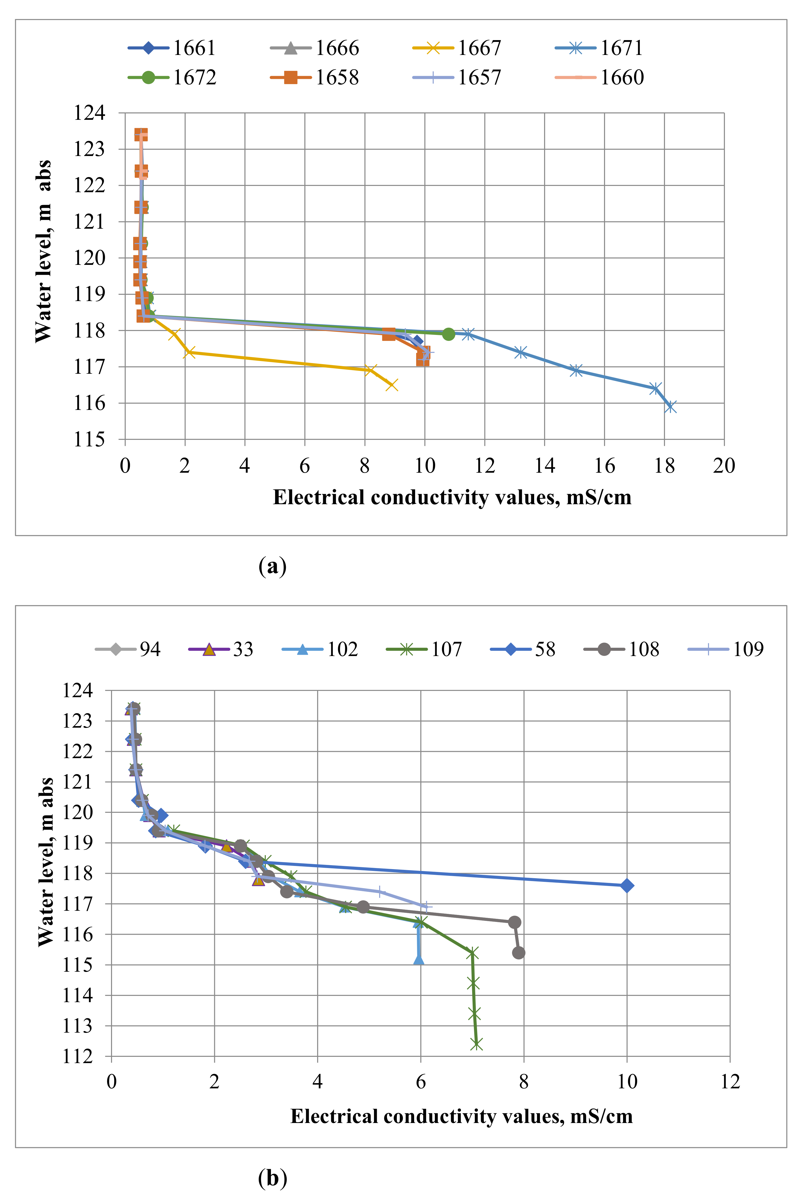
The results of the chemical sampling are in good agreement with the results of the conductometric survey of the Verkhne-Zyryansk reservoir’s water, and confirm the presence of saline waters in the bottom layer. All measurements of the electrical conductivity of water were carried out in two stages: on the 24 and 25 March 2020 (during the winter low-water period), and on the 15 and 16 July 2020 (during the summer low-water period).

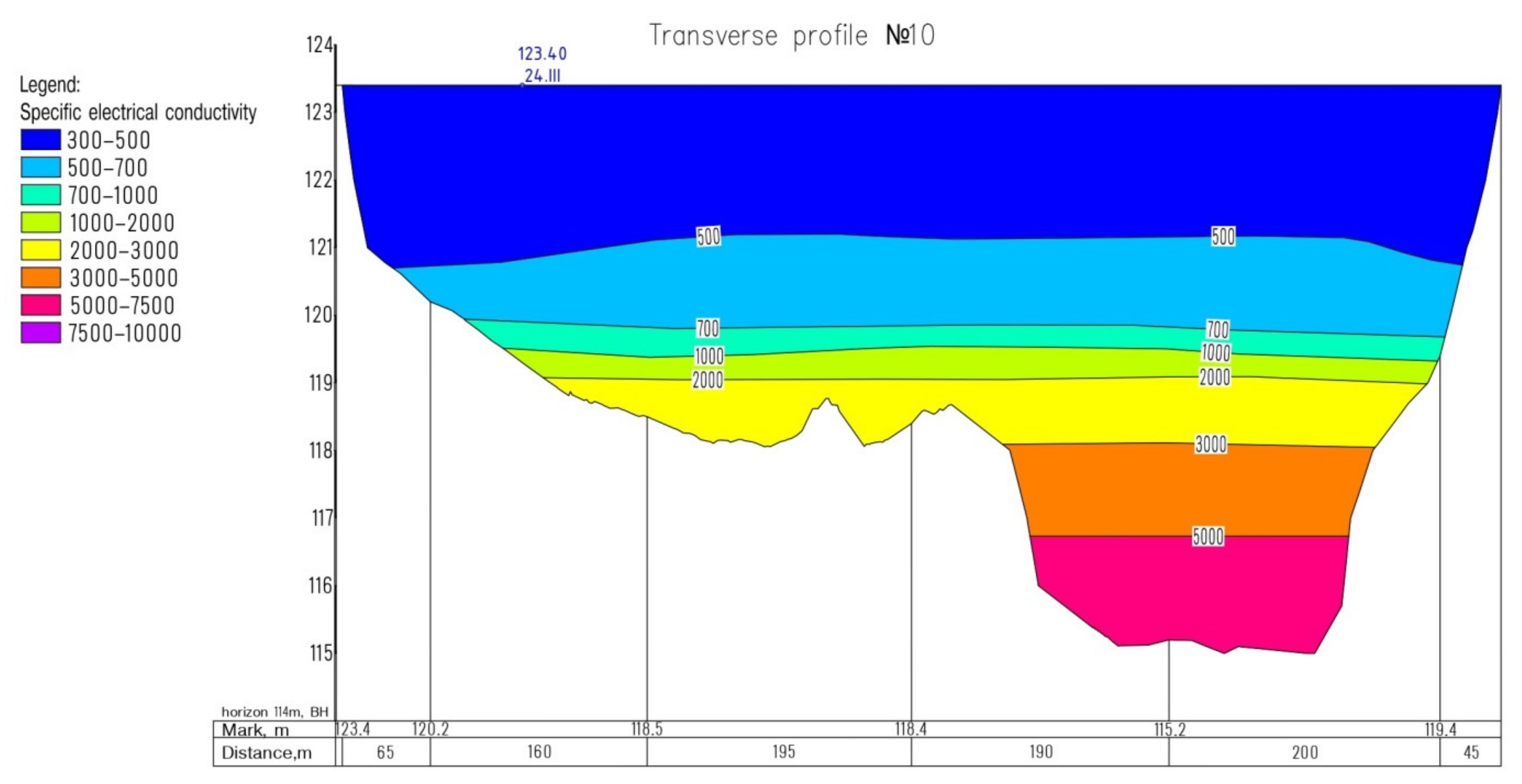
The results of fieldwork carried out in 2020 are presented in Figure 5 and Figure 6. Figure 5 shows the transverse profile of the distribution of the specific electrical conductivity (μS/cm) obtained in the water area of the Verkhne-Zyryansk reservoir during the winter low-water period.

Over the fifty plus years of operation of the Verkhne-Zyryansk reservoir, a considerable amount of pollutants, including the macrocomponents of the salt composition, gradually accumulated in its bottom layer. The alignment of the BKPRU-4 intake head location does not affect the specific electrical conductivity, which remains stable and does not change with a distance to the density jump layer. In this area, in terms of specific electrical conductivity for water salinity, the total salinity remained at the level of 0.3–0.4 g/L. During the year, the location of the density jump layer varies within ~1–1.5 m. In the summer period, it is located at the level of 118–119 m abs, below the location of the water intake head. In the winter, due to a change in the feeding regime of the water body and an increase in the proportion of the underground component, the level of the density jump increases up to 120–121 m abs. The water intake head is located at an elevation of 121 m abs. Thus, the density jump layer is very close to the horizon of the BKPRU-4 water intake head, while the water salinity at the considered depth increases to values of 0.5–0.6 g/L, exceeding the permissible standards for technical water supply.

3. Computational Experiment: Description and Mathematical Model

In view of the above considerations, there is a need for the construction of selective water intake to ensure the sustainability of the water supply from this water body. The peculiar features of the development of such water intake and the assessment of the possibility of reservoir flushing after the completion of the spring flood are discussed in [31,32]. To analyze the possible modes of sediment flushing, a series of computational experiments was carried out by coupling 2D and 3D hydrodynamic models. This calculation scheme has already been successfully used for solving specific water management problems in [31,33].

To construct a hydrodynamic model in a 2D formulation, a specialized software product, SMS v.11.1 of the American AQUAVEO LLC company (Provo, USA), was used [34]. Three-dimensional numerical modeling was carried out using the ANSYS Fluent package (ANSYS, Inc., Canonsburg, Pennsylvania, USA) based on the implementation of the finite volume method.

In the 2D simulations, the Reynolds-averaged Navier-Stokes equations for turbulent flows were solved by the finite element method. Friction was calculated using the Manning or Shezy formula, and the turbulent viscosity coefficients were used to characterize the turbulence. Since the design of the reservoir spillway allowed water retrieval from only the upper layer to the mark, it was very important to evaluate the flow structure at different discharge rates.

In 2D simulations, model RMA2 is a free-surface calculation model for subcritical flow problems. More complex flows, where vertical variations of variables are important, should be evaluated using a 3D model.

The generalized computer program RMA2 solves the depth-integrated equations of fluid mass and momentum conservation in two horizontal directions. The forms of the solved equations are:

$$h\frac{\partial u}{\partial t}+hu\frac{\partial u}{\partial x}+hv\frac{\partial u}{\partial y}-\frac{h}{\rho }\left[E_{xx}\frac{{\partial }^{2}u}{\partial x^2}+E_{xy}\frac{{\partial }^{2}u}{\partial y^2}\right]+gh\left[\frac{\partial a}{\partial x}+\frac{\partial h}{\partial x}\right]+\frac{gu{n}^2}{h^{\raisebox{1ex}{$1$}\!\left/ \!\raisebox{-1ex}{$3$}\right.}}{\left(u^2+v^2\right)}^{\raisebox{1ex}{$1$}\!\left/ \!\raisebox{-1ex}{$2$}\right.}-\zeta V_a^2\cos \psi -2hv\omega \sin \mathsf{\Phi }=0$$

(1)

$$h\frac{\partial v}{\partial t}+hu\frac{\partial v}{\partial x}+hv\frac{\partial v}{\partial y}-\frac{h}{\rho }\left[E_{yx}\frac{{\partial }^{2}v}{\partial x^2}+E_{yy}\frac{{\partial }^{2}v}{\partial y^2}\right]+gh\left[\frac{\partial a}{\partial y}+\frac{\partial h}{\partial y}\right]+\frac{gv{n}^2}{h^{\raisebox{1ex}{$1$}\!\left/ \!\raisebox{-1ex}{$3$}\right.}}{\left(u^2+v^2\right)}^{\raisebox{1ex}{$1$}\!\left/ \!\raisebox{-1ex}{$2$}\right.}-\zeta V_a^2\sin \psi +2hu\omega \sin \mathsf{\Phi }=0$$

(2)

$$\frac{\partial h}{\partial t}+h\left(\frac{\partial u}{\partial x}+\frac{\partial v}{\partial y}\right)+u\frac{\partial h}{\partial x}+v\frac{\partial h}{\partial y}=0$$

(3)

where h is water depth, u and v are velocities in the Cartesian directions, x, y, and t are Cartesian coordinates and time, ρ is the density of fluid, E is the eddy viscosity coefficient (for xx: normal direction on x-axis surface, for yy: normal direction on y-axis surface, for xy, and for yx: shear direction on each surface), g is acceleration due to gravity, a is elevation of the bottom, n is Manning’s roughness n-value, ζ is the empirical wind shear coefficient, Va is the wind speed, ψ is the wind direction, ω is the rate of earth’s angular rotation, and Φ is the local latitude.

Equations (1)–(3) were solved by the finite element method using the Galerkin method of weighted residuals. The elements may be one-dimensional channel reaches or two-dimensional quadrilaterals or triangles, and may have curved (parabolic) sides. The shape (or basis) functions are quadratic for velocity and linear for depth. Integration in space was performed by Gaussian integration. Derivatives in time were replaced by a non-linear finite difference approximation. The variables are assumed to vary over each time interval in the form:

$$f\left(t\right)=f\left(t_0\right)+at+b{t}^c\hspace{1em}{t}_0\le t<t_0+\Delta t$$

(4)

which is differentiated with respect to time and cast in finite difference form. Letters a, b, and c are constants. It was found by experimentation that the best value for c is 1.5 [35].

The solution is fully implicit and the set of simultaneous equations is solved by Newton-Raphson non-linear iteration scheme. The computer code executes the solution by means of a front-type solver, which assembles a portion of the matrix and solves it before assembling the next portion of the matrix.

The calculations were carried out for three different scenarios of water flow through the dam (

Table 2. The numerical setup used for 2D and 3D simulations.

Scenario No.	Intake Flow Rate m3/s	Intake Water Solute Concentration, g/L	Wind Velocity, m/s
1	0.30	0.30	0
2	2.04	0.30	0
3	8.51	0.30	0

): the minimum rate of water discharge, corresponding to the sanitary release, was 0.3 m³/s, the long-term average was 2.04 m³/s, and the average monthly discharge for the month of May, the time of spring flood, was 8.51 m³/s.

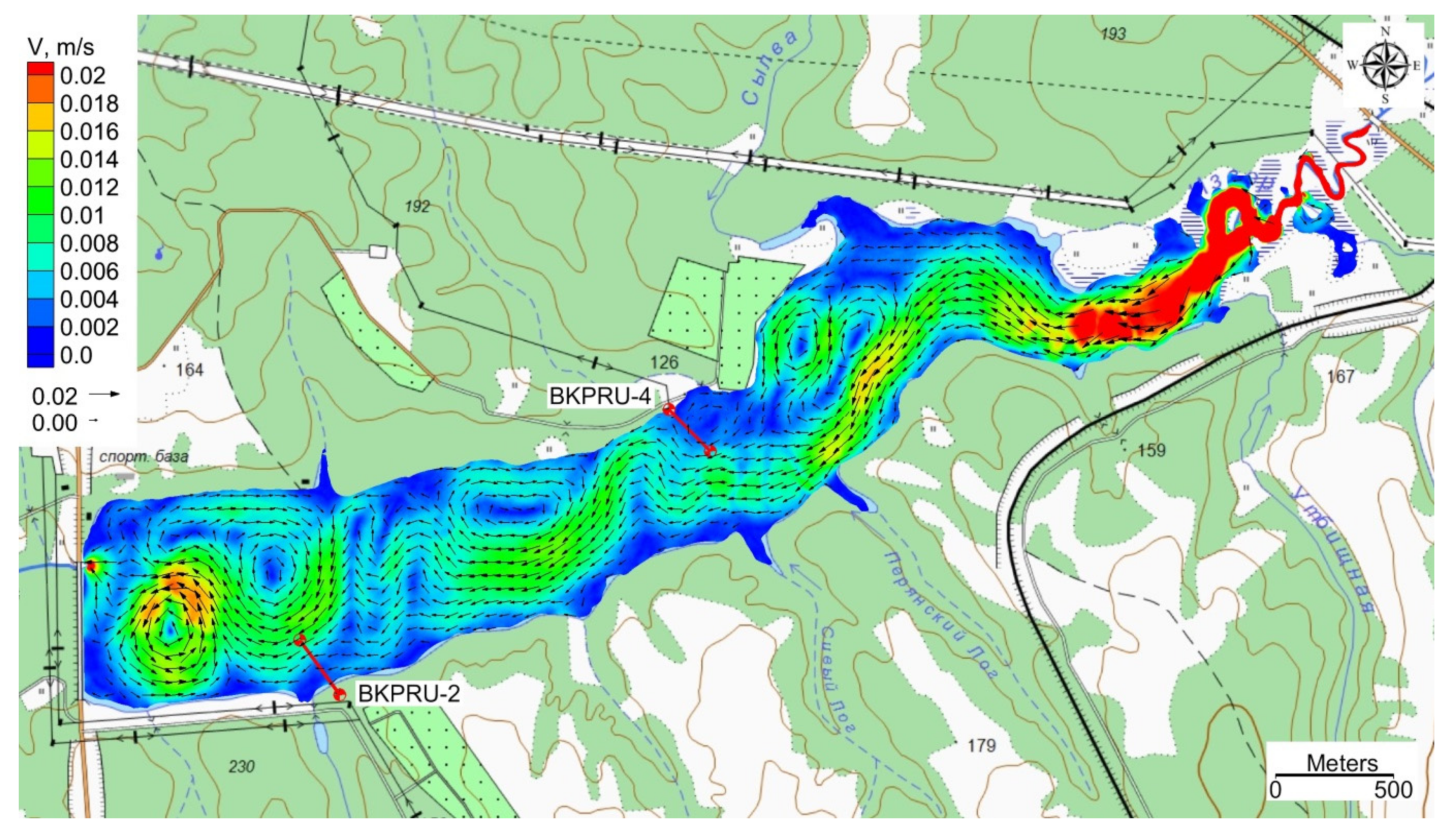
Of considerable practical interest is the assessment of the stability of the vertical non-uniformity of water masses, which, according to estimates [36], is maintained when the Froude number is Fr_ρ = 1 and the Richardson number is Ri >1.5. In the framework of the 2D hydrodynamic model, the calculations of the distribution of the flow velocity fields over the entire water area of the examined water body, including the water of the intake heads, were carried out for all three scenarios.

The calculations showed that, even at the time of the spring flood, the flow velocities are very low (Figure 7). Moreover, they are also slow during average annual discharges or sanitary releases (

Table 3. Calculated values of the average velocity in the area of the head of the BKPRU-4 water intake at the corresponding scenario water flow rates along the Zyryanka River. Two-dimensional simulation results.

Scenario No.	Water Flow Along the Zyryanka River, m3/s	Average Flow Rate at the Head of the BKPRU-4 Water Intake, cm/s
1	0.30	0.10
2	2.04	0.19
3	8.51	0.48

).

Such low flow rates under the conditions of diffuse pollution facilitate the formation of vertical heterogeneity of the water masses in the reservoir, which remain stable even during the spring flood. These estimates were verified by the results of the computational experiments carried out in a 3D formulation. All of the main water users are situated in the lower area of the reservoir, which significantly simplifies 3D modeling, as only its lower, deepest part was taken as the computational domain. In this case, the boundary conditions were specified based on the results of 2D calculations carried out for the entire reservoir (Figure 7).

To examine the effect of the flow rate of water passing through the dam on the position of the layer of the depth-wise mineralization jump, a 3D numerical simulation was carried out. A model problem was considered for the real geometry of the examined system (Figure 3), extending 3100 m along the channel with a maximum depth of 11 m. To construct the computational grid, the modeling area shown in Figure 8 was divided into quadrangular cells with a linear size of 20 m across the water area. The computational grid was built for three cases and consisted of a constant number of vertically located nodes: 80, 120, and 150. Morphometry was considered in terms of the compression and expansion functions. The test calculations showed that the grid containing 120 nodes was optimal for computations. This is depicted in Figure 8b with 80× vertical magnification.

In our simulation, we used a computational grid with the refinement towards the bottom of the reservoir; the maximum size was 0.3 m and the minimum size was 0.02 m, while the number of nodes was 80 along the vertical. The total number of nodes in the computational grid was 670,000.

At the initial moment of time, the inhomogeneous depth-wise distribution of concentration is defined in terms of the function as:

$$C\left(z\right)=\left\{\begin{array}{c}0.3 g/l, z>-4 \mathrm{m}, \\ 3 g/l, z\le -4 \mathrm{m}, \end{array}\right.\mathrm{z}=0 \mathrm{conforms} \mathrm{to} \mathrm{the} \mathrm{water} \mathrm{surface},$$

(5)

Water flows out at a constant velocity from the outlet of the dam by raising the shandor, the lower part of which is located at a depth of 4 m from the surface. At the inlet to the computational domain, a constant flow velocity was set, while the concentration was specified as a jump (5).

The calculations were carried out within the framework of a steady isothermal problem until a stationary solution was obtained with an accuracy of 3.5 × 10⁻⁴. The turbulent pulsations were described using the least resource- and time-consuming $k-\epsilon$ model. The quadratic dependence of the density on the concentration $\rho ={\rho }_0+A\cdot c+B\cdot c^2$ (${\rho }_0=999.993, A=667.8, B=-0.1229$) was considered. In this case, the depth-wise decrease of water density was 10%.

The equation for the balance of mass and momentum has the form:

$$\frac{\partial \rho }{\partial t}+\frac{\partial }{\partial x_i}(\rho {\mathrm{v}}_i)=0,$$

(6)

$$\begin{gathered} \frac{\partial }{\partial t}(\rho {\mathrm{v}}_i)+\frac{\partial }{\partial x_j}(\rho {\mathrm{v}}_i{\mathrm{v}}_j)=-\frac{\partial p}{\partial x_i}+\frac{\partial }{\partial x_j}\left[\mu \left(\frac{\partial {\mathrm{v}}_i}{\partial x_j}+\frac{\partial {\mathrm{v}}_j}{\partial x_i}-\frac{2}{3}{\delta }_{ij}\frac{\partial {\mathrm{v}}_l}{\partial x_l}\right)\right] + \\ +\frac{\partial }{\partial x_j}\left[{\mu }_t\left(\frac{\partial {\mathrm{v}}_i}{\partial x_j}+\frac{\partial {\mathrm{v}}_j}{\partial x_i}\right)-\frac{2}{3}\left(\rho k+{\mu }_t\frac{\partial {\mathrm{v}}_l}{\partial x_l}\right){\delta }_{ij}\right]+\rho g_i; \end{gathered}$$

(7)

Here, $\rho$ is the density of the fluid, ${\mathrm{v}}_i$ are the velocity components ($i=x,y,z$ are Cartesian coordinates), $x$ and $y$ are the horizontal coordinates, the main flow is directed along the $x$ coordinate, $z$ is the vertical coordinate, the $\mu$ is the kinematic viscosity of the fluid, and ${\delta }_{ij}$ is the Kronecker symbol. Turbulent viscosity ${\mu }_t$ is a function of turbulent kinetic energy $k$ and the rate of its dissipation $\epsilon$: ${\mu }_t=\rho C_{\mu }{k}^2/\epsilon$:, where $C_{\mu }$ is a constant.

The equations for the turbulent energy and its velocity are written in the form:

$$\frac{\partial }{\partial t}\left(\mathsf{\rho }k\right)+\frac{\partial }{\partial x_i}\left(\mathsf{\rho }k{\mathrm{v}}_i\right)=\frac{\partial }{\partial x_j}\left[\left(\mu +\frac{{\mu }_t}{{\sigma }_k}\right)\frac{\partial k}{\partial x_j}\right]+G_k+G_b-\mathsf{\rho }\epsilon ,$$

(8)

$$\frac{\partial }{\partial t}\left(\rho \epsilon \right)+\frac{\partial }{\partial x_i}\left(\rho \epsilon {\mathrm{v}}_i\right)=\frac{\partial }{\partial x_j}\left[\left(\mu +\frac{{\mu }_t}{{\sigma }_{\epsilon }}\right)\frac{\partial \epsilon }{\partial x_j}\right]+C_{1\epsilon }\frac{\epsilon }{k}{G}_k-C_{2\epsilon }\rho \frac{{\epsilon }^2}{k}$$

(9)

Here, $G_k={\mu }_t{S}^2$ is the generation of turbulent kinetic energy due to the average velocity gradient; $S=\sqrt{2S_{ij}{S}_{ij}}$ is the norm of the tensor of the average rate of deformation of the flow, $S_{ij}=\frac{1}{2}\left(\frac{\partial {\mathrm{v}}_j}{\partial x_i}+\frac{\partial {\mathrm{v}}_i}{\partial x_j}\right)$; ${\mathrm{Pr}}_t$ is the turbulent Prandtl number; and $C_{1\epsilon },C_{2\epsilon },{\sigma }_k,{\sigma }_{\epsilon }$ are the constants.

The equation for turbulent kinetic energy includes the term $G_b=-\frac{g_j({\mu }_t/\rho )}{{\mathrm{Pr}}_t}\frac{\partial \rho }{\partial x_j}$, which describes the generation of turbulent energy due to buoyancy forces in the gravity field. In the case of stable density stratification $\frac{\partial \rho }{\partial x_3}<0$, the gravitational acceleration vector $\overrightarrow{g}$ is directed vertically downward and the above term is negative, which means a decrease in turbulent kinetic energy due to buoyancy.

The applicability of the $k-\epsilon$ turbulence model was verified by performing test calculations using a higher order model, the Reynolds model, in which seven additional equations for the Reynolds stresses are solved. It was found that for different grids, the difference in the obtained data was less than 5% for the integral values of the velocity components in different sections.

The solute transport equation is written in the form:

$$\frac{\partial }{\partial t}\left(\rho c\right)+\nabla \cdot \left(\rho v c\right)=-\nabla \cdot J$$

(10)

Where $\nabla$ is the nabla operator and $J$ is the vector of the diffusion solute flux, determined by the expression:

$$J=- \rho \left(D_m+D_t\right)\nabla c,$$

(11)

where $D_m$ is the molecular diffusion coefficient, $D_t$ is the effective turbulent diffusion coefficient, related to the turbulent viscosity ${\mu }_t$ by the ratio $D_t=\left({\mu }_t/\rho \right)/{\mathrm{Sc}}_t$, and ${\mathrm{Sc}}_t$ is the turbulent Schmidt number.

The parameters used in Equations (6)–(11), ${\mathrm{Pr}}_t$, $S{c}_t$, $G_{1\epsilon }$, $C_{2\epsilon }$, $C_{\mu }$, ${\sigma }_k$ and ${\sigma }_{\epsilon }$, are empirical constants and their values were taken from [37], where: ${\mathrm{Pr}}_t=0.85$, $S{c}_t=0.7$, $C_{1\epsilon }=1.44$, $C_{2\epsilon }=1.92$, $C_{\mu }=0.09$, ${\sigma }_k=1.0$, and ${\sigma }_{\epsilon }=1.3$. The kinematic viscosity was taken as equal to $\mu =9.34\times {10}^{-7}{\mathrm{m}}^2/\mathrm{s}$, and the molecular diffusion coefficient was $D=1.0\times {10}^{-9}{\mathrm{m}}^2/\mathrm{s}$.

The boundary conditions for Equations (6)–(11) are provided below for different boundaries of the system.

We have imposed the no-slip and zero mass flux conditions on the rigid boundaries (river bottom and banks):

$${\mathrm{v}}_x={\mathrm{v}}_y={\mathrm{v}}_z=0,\hspace{1em}\frac{\partial c}{\partial n}=0;$$

(12)

At the entrance to the computational domain, the velocity of the main flow was set (the vector of the flow velocity of the environment is perpendicular to the inlet boundary $\overrightarrow{U}=\left\{U, 0, 0\right\}$), and the concentration was set as equal to the background concentration of the pollutant in water:

$${\mathrm{v}}_x=U,\hspace{1em}{\mathrm{v}}_y=0,\hspace{1em}{\mathrm{v}}_z=0,\hspace{1em}c=c_0$$

(13)

The upper boundary of the computational domain, corresponding to the free surface of the liquid, was assumed to be non-deformable and was subjected to the condition for the absence of the normal component of the velocity, tangential stresses, and solute flux:

$$(v n)=0, \frac{\partial {\mathrm{v}}_x}{\partial x_z}+\frac{\partial {\mathrm{v}}_z}{\partial x_x}=0, \frac{\partial {\mathrm{v}}_y}{\partial x_z}+\frac{\partial {\mathrm{v}}_z}{\partial x_y}=0, \frac{\partial c}{\partial n}=0$$

(14)

The mass balance condition prescribed at the outlet of the computational area is given as:

$${\displaystyle \underset{S_{in}}{\oint }\rho {\mathrm{v}}_{in}dS}-{\displaystyle \underset{S_{out}}{\oint }\rho {\mathrm{v}}_{out}dS}=0;$$

(15)

For the coefficient of river bottom roughness, we used a value of 0.035 (the average sand size taken from field data), which corresponds to the sand grain surface homogeneity and the roughness height of 0.001 m. To discretize the equations in space, the second-order accuracy scheme was used. We applied cell-centered structured finite-volume discretization and least square cell-based for spatial discretization. The time derivative was discretized using backward differences by the second-order discretization. ANSYS Fluent uses the multi-stage Runge-Kutta explicit time integration.

We investigated the scenarios of water flow, for which the velocity regimes were determined using a 2D approach (Table 2). The input velocity was determined based on the data of the 2D calculations.

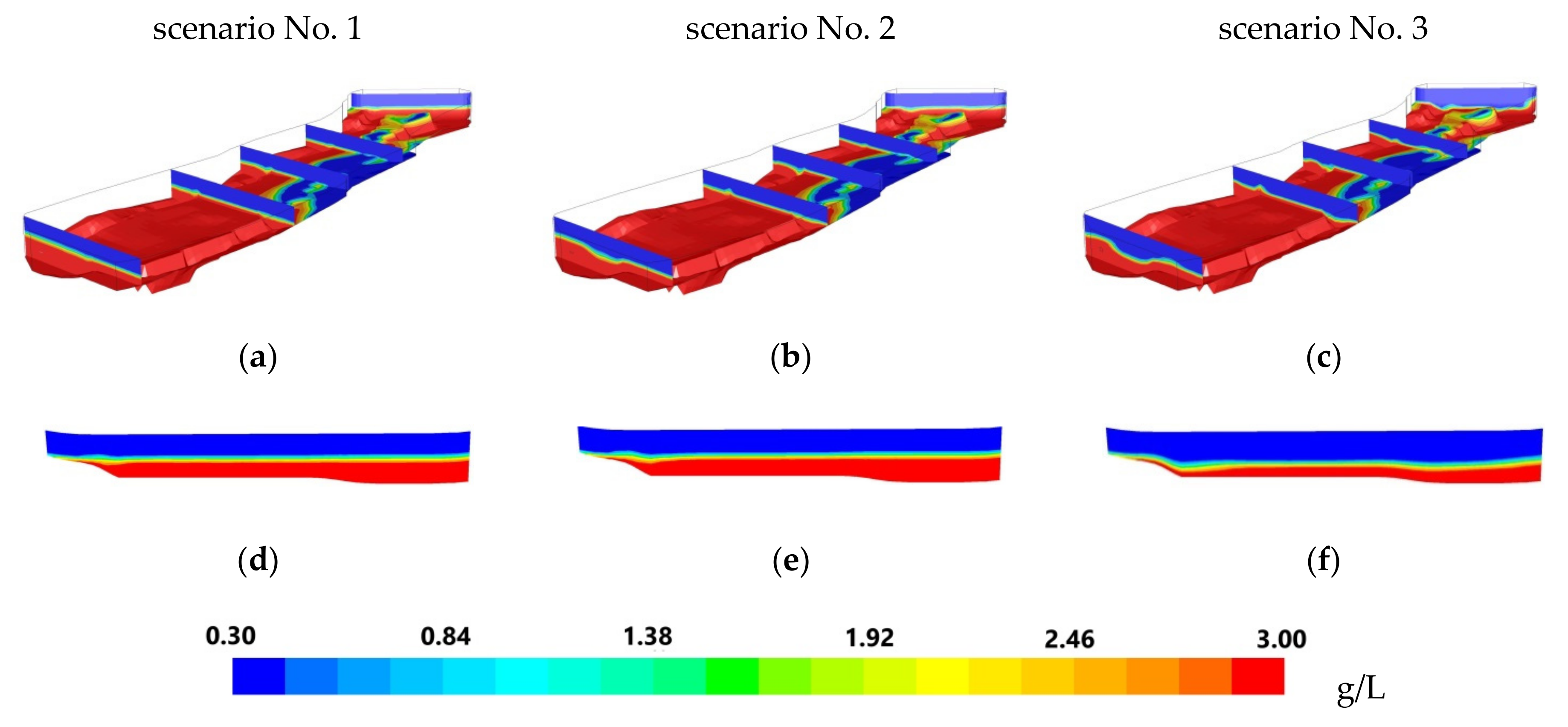
The results of the numerical experiments provided a clear understanding of the intra-annual fluctuations in water salinity observed at the BKPRU-4 water intake. After the spring flood is over, the deposited sediments are flushed out from the reservoir. As a result, the height of the density jump layer decreases, which reduces water salinity entering the water intake head (scenario No. 3 in Figure 9).

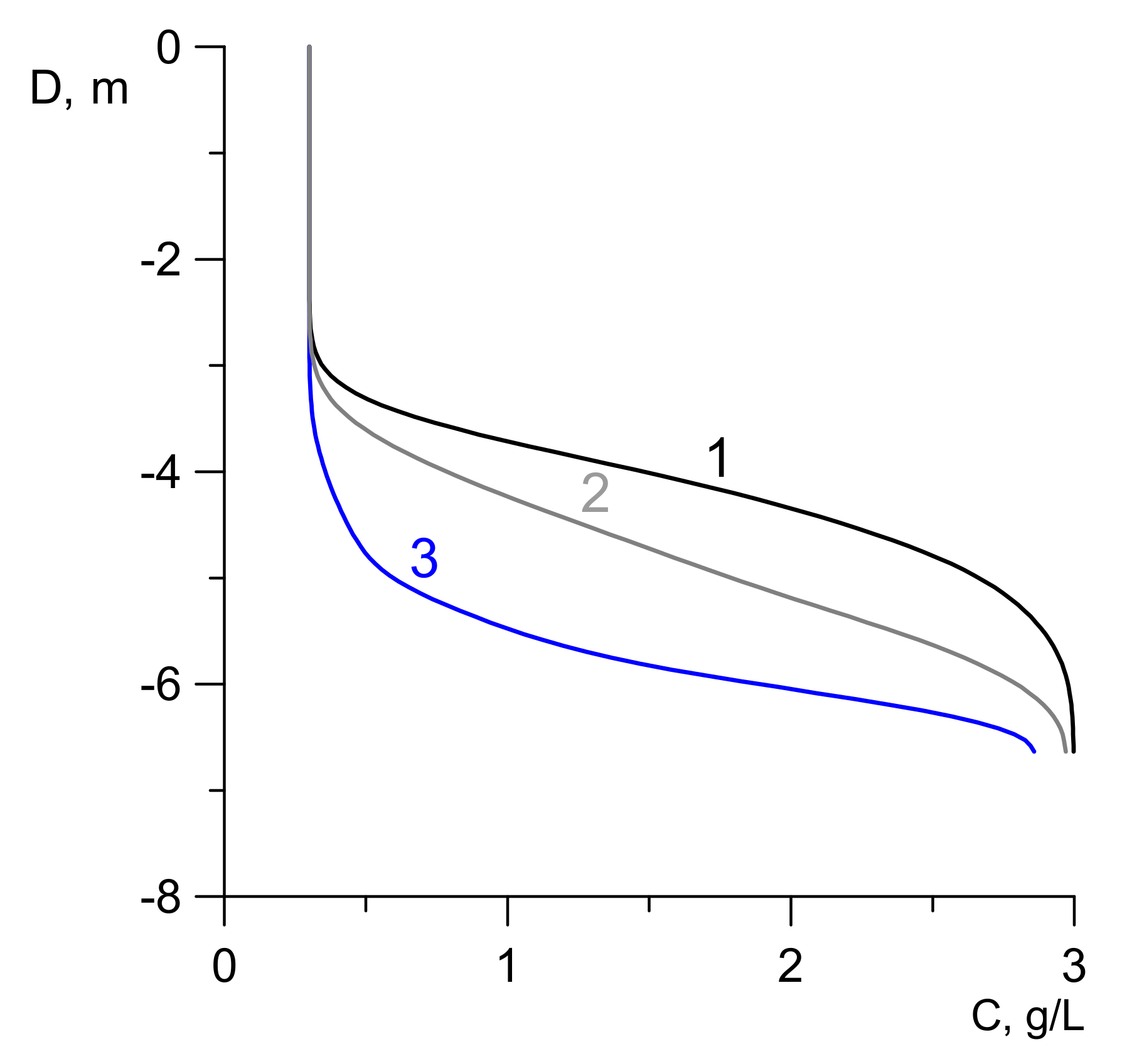
During the summer and, especially, the winter low-water period, due to the low-water discharges, the height of the jump layer increased (scenarios Nos. 1 and 2 in Figure 9) and the salinity of the withdrawn water increased. The behavior of the jump layer for different water flow rates, along a separate vertical of the reservoir near the water intake, is shown in Figure 10. A significant increase in the water flow rate impedes the removal of the accumulated salt from the bottom, which causes a decrease in the jump layer as shown by curve 3 in Figure 10.

The data obtained make it possible to find a solution to the problem of a sustainable water supply from this reservoir. The distribution of salinity would be significantly different if the culvert was located 2 m below the actual configuration. With a deeper spillway location, a much more efficient flushing would occur, which would restrict the location of zones of increased mineralization to individual local bottom reliefs and, essentially, improve the quality of the water taken.

4. Discussion

In water bodies located in zones of active technogenesis characterized by dispersed, diffuse sources of pollution, the low flow velocities are responsible for the formation of stable vertical density stratification. In this case, the specific electrical conductivity, and the salinity of water in the lower bottom horizons, can almost reach an order of magnitude higher than their values in the surface layer. As shown in [36], a stable vertical structure is formed and observed at the density of Froude numbers at Fr_ρ <1.5. The phenomenon of vertical density stratification of water masses caused by the inhomogeneous distribution of both temperature and mineralization has long been a hotly debated issue [12,13,14,15,16,17,18,19,20,21,22,23,24,25,26,27,28,29,30,31,32].

In the present paper, using the specific example of the Verkhne-Zyryansk reservoir, we considered the effect of vertical density stratification, formed as a result of uncontrolled, diffuse pollution, on the stability of the intake system providing technical water supply from this reservoir. It was shown that the traditional system of organizing water intakes, which are built under the assumption of the vertical homogeneity of water masses, cannot ensure their reliable operation in winter. The weirs, designed according to the condition of vertical homogeneity of water masses, cannot provide effective washing of this water body. Therefore, in order to prevent this negative phenomenon at the design stage, it is necessary to select a location for the weir threshold which would allow for the effective washing of the zones of the intake header location. In cases where weir reconstruction is impossible, the selective water intake can be realized by changing the design and location of the water intake.

Monitoring can provide an effective assessment of the state of the water body under consideration only under specific observation conditions. At the same time, in order to solve specific problems of the sustainable, economic use of a water body, it is necessary to analyze situations under possible extreme hydrological regimes.

This problem can be effectively solved by carrying out computational experiments based on hydrodynamic models. The use of traditional shallow water models for these purposes is not justified since they require vertical homogeneity of the water masses. The use of 3D models in the hydrostatic approximation can be ineffective due to the complex morphometry of the water body under consideration. At the same time, 3D hydrodynamic models in the full, non-hydrostatic approximation require very significant computational resources. For this reason, a combined scheme was used in the present paper based on the coupling of the 2D and 3D hydrodynamic models. Previously, this was successfully used to solve a number of topical, applied problems [20,31,32,33,38].

The developed model efficiently reproduces the location of the interface between water masses and its changes depending on the hydrological regime of the reservoir. The expected outcome of this model was the assessment of the possibility of water body flushing at extremely high-water flow rates. The calculations showed that, due to the design features of the culvert, washing of the reservoir is impossible. Therefore, to ensure a sustainable technical water supply, it was proposed to reconstruct the heads of the water intake device. Since the process of the formation of the lower water layer’s increased salinity is rather inertial, it is necessary to provide timely detection of this highly unfavorable phenomenon by means of creating an effective monitoring system for water bodies which consider the distribution of monitored indicators over the depth of the water body.

5. Conclusions

In the water bodies located in zones of active technogenesis, characterized by developed, dispersed, and diffuse sources of pollution, a steady state vertical density stratification is formed at low-flow velocities. A significant vertical inhomogeneity of the mineralization and water temperature distributions has a significant impact on the character of and effective use of these water bodies. This influence is most apparent in the designs of systems for taking water of a required quality, since water intakes within the bottom location of intake windows begin to take water of much poorer quality compared to that in the surface horizons. To prevent such negative phenomena, it is necessary at the design stage to determine the location of the weir threshold which would allow effective flushing in the zones where intake heads are located. In the case when the reconstruction of the weir is impossible, the selective water intake can be realized by changing the design and location of the water intake device.

It is advisable to study the design features of the water intake device on the basis of computational experiments in a 3D formulation. It should be emphasized that the hydrodynamic models of shallow water, which are currently used for solving the applied problems, have proven to be ineffective in this regard since they a priori assume the vertical non-uniformity of water masses. They can be used as a highly effective auxiliary tool in the construction and implementation of 3D hydrodynamic models in the non-hydrostatic approximation. Such an approach, based on the conjunction of hydrodynamic models in 2D and 3D formulations, allows for a significant reduction of the required computational resources.