
Decision Support Model for Ecological Operation of Reservoirs Based on Dynamic Bayesian Network


1
Changjiang River Scientific Research Institute, No. 23 Huangpu Road, Wuhan 430010, China
2
College of Hydrology and Water Resources, Hohai University, No. 1 Xikang Road, Nanjing 210098, China
3
College of Civil Engineering and Architecture, Zhejiang University, No. 866 Yuhangtang Road, Hangzhou 310058, China
*
Author to whom correspondence should be addressed.
Water 2021, 13(12), 1658; https://doi.org/10.3390/w13121658
Submission received: 21 March 2021
/
Revised: 7 June 2021
/
Accepted: 8 June 2021
/
Published: 14 June 2021
(This article belongs to the Section Hydrology)
Abstract
:In this study, a model was proposed based on the sustainable boundary approach, to provide decision support for reservoir ecological operation with the dynamic Bayesian network. The proposed model was developed in four steps: (1) calculating and verifying the sustainable boundaries in combination with the ecological objectives of the study area, (2) generating the learning samples by establishing an optimal operation model and a Monte Carlo simulation model, (3) establishing and training a dynamic Bayesian network by learning the examples and (4) calculating the probability of the economic and ecological targets exceeding the set threshold from time to time with the trained dynamic Bayesian network model. Using the proposed model, the water drawing of the reservoir can be adjusted dynamically according to the probability of the economic and ecological targets exceeding the set threshold during reservoir operation. In this study, the proposed model was applied to the middle reaches of Heihe River, the effect of water supply proportion on the probability of the economic target exceeding the set threshold was analyzed, and the response of the reservoir water storage in each period to the probability of the target exceeding the set threshold was calculated. The results show that the risks can be analyzed with the proposed model. Compared with the existing studies, the proposed model provides guidance for the ecological operation of the reservoir from time to time and technical support for the formulation of reservoir operation chart. Compared with the operation model based on the designed guaranteed rate, the reservoir operation model based on uncertainty reduces the variation range of ecological flow shortage or the overflow rate and the economic loss rate by 5% and 6%, respectively. Thus, it can be seen that the decision support model based on the dynamic Bayesian network can effectively reduce the influence of water inflow and rainfall uncertainties on reservoir operation.
1. Introduction
River ecological flow management has attracted increasing attention of many researchers in recent years. Poff and other 19 scholars [1] jointly put forward a new framework for developing regional environmental flow standards, namely the ecological limits of hydrologic alteration (ELOHA). ELOHA is a mixture of existing hydrologic techniques and environmental flow methods that can support the comprehensive regional flow management. Under the ELOHA framework, the scientific and testable relationships between the hydrologic alteration and the ecological responses were established and used to develop the regional flow management standards. Even though ELOHA has balanced the scientific rigor and the application cost of many rivers in setting environmental flow standards, many governments could not (or would not) afford to apply ELOHA (typically ranging from $100,000 to $2 million) [2]. In addition, ELOHA could not be applied to many areas with low spatial coverage of biological data. Therefore, Richter et al. [2,3] proposed the sustainable boundary approach (SBA) as a reference for the ecological flow management of these areas. The SBA, which is extended from the “percent-of-flow” approaches, proposes to set an allowable variation range called sustainable boundaries around the natural flow conditions as an approach to express the requirements of environmental flow management. For comparison with the previous methods in terms of technology, the SBA protects the variability of flow (which cannot be realized by the minimum threshold method) without requesting excessive professional demands on water managers (complex statistical methods are difficult for water managers to perform). From a management perspective, the SBA views the protection of ecological flows as an integrated sustainable management of water resources instead of water allocation merely. Some scholars [4,5] have proved that the SBA provides sufficient protection for river ecology and also some guidance for river classification, so as to balance the scientific rigor and the practicality. In the opinion of authors, SBA has the advantages of operability and protections for river ecology, which make it a suitable ecological objective for uncertainty analysis.
However, in our opinion, the formulation of sustainable boundary is only the first step in ecological flow management. There are still many choices to be made within the sustainable boundaries, such as the trade-off between ecological and water supply. The sustainable boundary is established from the ecological perspective, regardless of economic benefits. In fact, ecological flow management measures are difficult to implement regardless of economic benefits and participation of stakeholders. Since ecological flow management is viewed as an integrated management of water resources, it is necessary to establish a decision support model for water withdrawal to cooperate with the SBA for flow management. Two important challenges that should be overcome are: (i) the response relationship between the flow and river ecosystem and (ii) the multi-objective coordination between the ecological and economic objectives [6,7]. However, these challenges are not addressed in this study. Authors believe that for policy-makers, although the value of ecological objectives is difficult to quantify, it is relatively easy to compare the unacceptable degree of economic loss and ecological loss risk. Therefore, this study considered the probability of ecological and economic targets exceeding the set threshold as the basis of reservoir water withdrawal decision. It can provide a new idea for the decision of reservoir operation.
Uncertainty is a universal concept in the objective world. The inflow runoff, water demand and engineering characteristics affecting the operation of a reservoir are mostly uncertain and hence it is of great significance to study the risks of reservoir operation. In the 1980s, Hasan [8] put forward the concept and analysis method of risk in reservoir operation. However, this method has some drawbacks for the following two reasons. First of all, the traditional method mostly calculates the risk based on the prior probability of uncertainty through the statistical method, but the uncertainty of reservoir operation changes with time. Hence, a dynamic model should be established for the integrated operation process of reservoirs. Second, it is difficult to obtain the high-dimensional nonlinear joint probability distribution function composed of multiple uncertain factors by the traditional method. Therefore, Pearl [9] put forward the Bayesian network (BN), to obtain the high-dimensional nonlinear joint probability distribution.
BN is a probabilistic inference and diagnosis network based on Bayesian condition probability and graph theory [10]. With the causal relationship between each node defined, the risk events were represented as the directed acyclic graphs that consist of the nodes and the directed arcs. Nodes in BNs represent the stochastic variables, whereas the arcs represent the causal relationships between the variables. Lack of arcs between two nodes represents the conditional probabilistic independence of the two variables [11]. In this way, the dimension reduction of joint probability distribution function can be realized by conditional independence between random variables. Owing to these characteristics, BN models are very suitable for simulating systems that are difficult to be simulated by the mechanistic models. The BN model has been widely applied in the domains of dam risk analysis, weather forecast, intelligent informatics and water management assessment [12,13,14,15,16]. In the field of reservoir ecological operation, Pang et al. [17,18] proposed an environmental flow decision-making method based on BN and carried out a trade-off analysis between ecological environment flow and agricultural economic losses with the static BN to determine the ecological environment flow. Xue et al. [19] proposed a decision-making framework to calculate the environmental flow requirements based on the static BN.
However, it is not enough to put forward a total ecological water demand in the ecological operation of a reservoir, as it is a dynamic process. For example, the prediction error of reservoir inflow changes with time. The uncertainty of each objective is in connection with the real-time reservoir storage, which changes with time as well. Therefore, the uncertainty in reservoir operation not only has the characteristics of uncertainty itself, but also has time variability. Thus, scientific decisions can be made on the water supply in the current period by considering the water storage, water inflow and water demand.
The traditional static BN model is difficult to simulate a system with dynamic process or too many system variable values. Hence, (i) the flow management process cannot be detailed in the existing research (only an overall goal can be proposed) and (ii) the decision-maker cannot adjust the decision according to the existing information. Herein, a dynamic Bayesian network (DBN) was introduced to dynamically model the reservoir operation process. DBNs connect several static BNs with time extension to simulate and analyze the dynamic process. If there is a dynamical component in the system that needs to be controlled (such as a reservoir or water intake engineering), the number of alternatives to be examined is very high due to the combinatory effects. Therefore, the decision support model also needs the help of mathematical programming or optimal control model [11,20]. The DBN model was initially applied to the speech recognition, probability prediction and gene network inference and improvements in machine learning algorithms [21,22,23,24]. In recent years, some researchers have applied the DBN model to water resource management. Chen [14] also calculated and analyzed the uncertainty in flood control operation of reservoirs with DBN.
Pang and Xue et al. [17,18,19] used Bayesian network model to calculate the recommended ecological flow for reservoir operation, but the recommended ecological flow only follows the static reservoir operation rule. The advantages of dynamic regulation in reducing the uncertainty of reservoir operation compared with static rules will be discussed in the Section 4. Chen [14] applied DBN to reservoir flood control operation. However, Chen’s research only considered the single goal of flood control, and there were many targets in the utilizable benefit operation of reservoir, which made the above research could not be applied in the comprehensive utilization operation of the reservoir. In addition, for ecological operation and flood control, various factors should be considered. For example, flood risk can be calculated based on the current level of water in front of the dam, whereas the uncertainty of economic losses is related not only to the current amount of water supplied, but also to the amount supplied in previous periods. On the basis of the above research, a DBN model and an economic optimization model were established. Meanwhile, the dynamic adjustment strategy of reservoir was applied to the integrated operation of a reservoir. In this paper, the operation objectives of ecological and economic loss were considered, and the calculation of the exchange ratio of the uncertainty of two objectives provides scientific guidance for the integrated operation of reservoirs.
In order to provide guidance for the ecological operation of reservoirs from time to time, the ecological sustainability boundaries and economic loss threshold are first established as the ecological and economic objectives of reservoir operation. Then the dynamic simulation and evaluation of the reservoir operation was carried out with the deterministic optimization model as the learning samples of DBNs. Finally, a DBN model was established and trained according to the expert knowledge and learning samples. Through this model, the decision-maker can take the uncertainty of reservoir operation as a consideration to analyze the water intake of the reservoir and formulate the regulation of the reservoir. It provides a new point of view for solving the water-use contradiction between different time and different target in water shortage area.
2. Methods
2.1. Methodological Framework
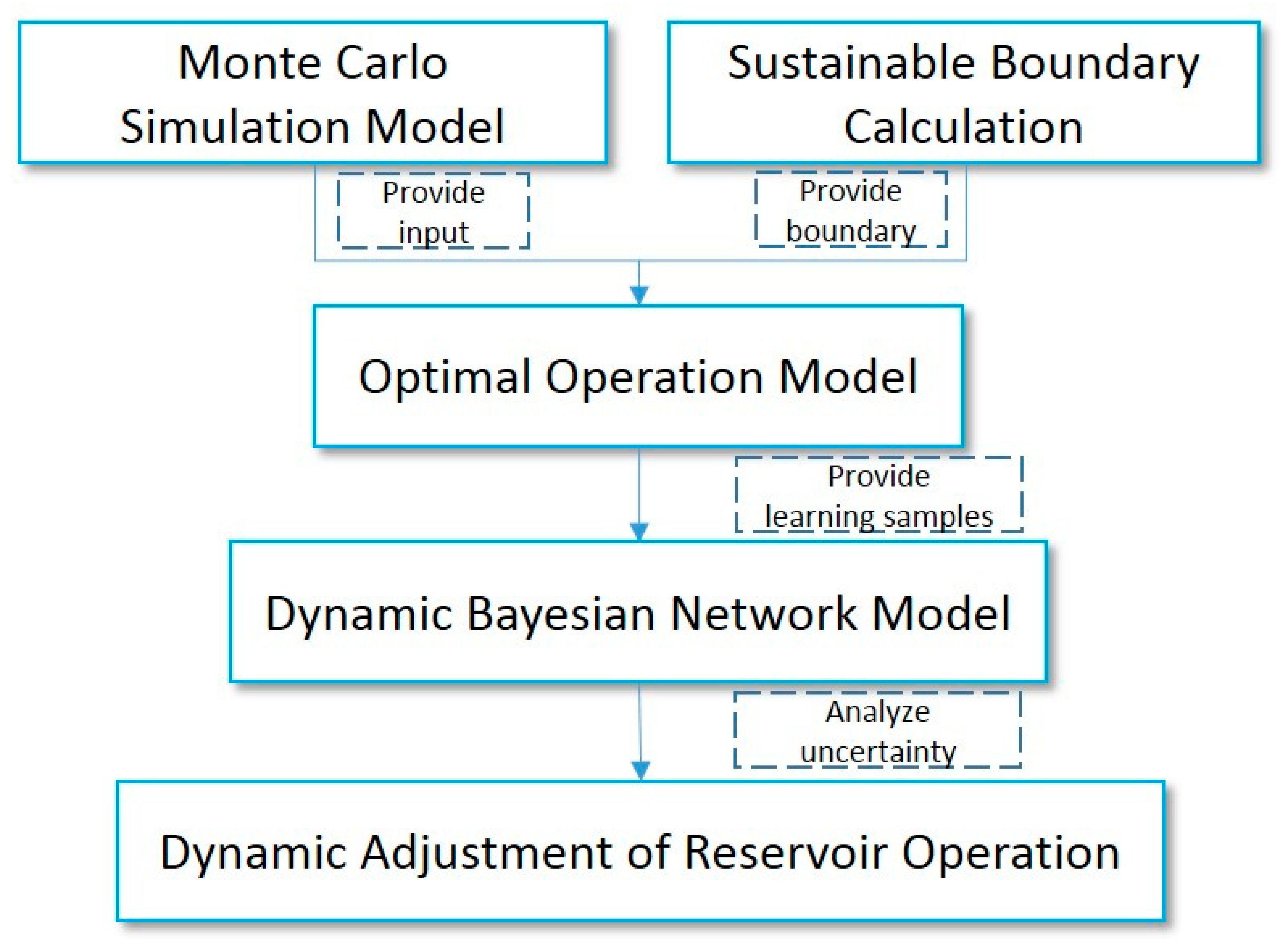
As the inflow and demand of reservoir ecological operation change with time, the states of each node in BN also change with time. Therefore, it is necessary to simulate the operation process of the reservoir through deterministic optimization model to generate DBN learning samples. As Figure 1 shows, the proposed model has four parts: (i) formulation of sustainable boundaries, (ii) establishment of an optimal operation model, (iii) establishment of DBN and (iv) decision support based on risk analysis.
Sustainable boundaries could provide adequate protection of the hydrological regime of the river. At the same time, using sustainable boundaries as the ecological target of reservoir operation can reduce the difficulty of solving the model and provide a basis for the calculation of ecological flow shortage and overflow rate. Sustainable boundaries provide boundary conditions for the optimization model. The random reservoir inflow, rainfall and crop prices are generated by Monte Carlo simulation based on the statistical parameters of the measured data and these data are used as inputs to the optimization model.
The economic optimization model sets the minimum economic loss as the target, the reservoir inflow, rainfall and crop price as the inputs, and the reservoir water supply as the decision variable, to calculate the optimal reservoir discharge process and the corresponding economic loss. The optimal operation model provides learning sample inputs for the DBN training.
The DBN model was established and trained according to the expert knowledge and learning samples. The probability that the ecological flow cannot be kept within the sustainable boundary and the probability that the economic loss cannot be kept within the set threshold are calculated by DBNs from time to time. The recommended water supply of the reservoir for each period was determined by the decision-maker’s acceptability of the ecological and economic targets.
The specific description for these parts of the model is explained in detail in the following sections.
2.2. Formulation of Sustainable Boundaries
Richter [2,3] suggested that the protection of environmental flows should be viewed as an integrated management of water resources for long-term sustainability, not as water distribution. From this point of view, the sustainable boundaries of ecological flow were established to protect the hydrological regime of rivers, and the ecological target is to maintain the flow within the sustainable boundaries. Maintaining the flow within the sustainable boundaries as the ecological target reduces the difficulty of solving as well as improves the computational speed of the model. At the same time, it provides a basis for the calculation of ecological flow shortage and overflow rate.
The SBA provides protection for river ecosystems by setting allowable percentages of deviation from the natural condition. In this work, the annual average natural daily flow is taken as the natural condition. Annual average natural daily flow refers to the flow process without artificial interference after the measured flow is calculated by reduction calculation such as adding artificial water taking and so on. Calculating the degree of allowable augmentation and depletion during the wet and dry seasons is the key to establishing sustainable boundaries. In this work, only ecological factors are considered in the formulation of sustainable boundaries. The ecological factors are considered from both inside and outside the river channel. The protection of ecological flow inside the river channel is evaluated by the range of variability approach (RVA). RVA [24,25,26,27] quantitatively analyze the deviation of ecological flow from the natural flow pattern using indicators of hydrologic alteration (IHA). The mathematical expressions are as follows:
where Ai is the degree of change of the ith index, N0(i) is the number of years in which the ith index is observed in the corresponding RVA target ranges, Ne(i) is the number of years in which the ith index is expected in the corresponding RVA target ranges, and A is the overall hydrological alteration.
The allowable percentages of deviation from the natural condition during the wet and dry seasons were taken as decision variables. This paper used simulation and genetic algorithm to calculate combinations of allowable percentages of deviation that can minimize hydrological alteration without increasing ecological flow [28]. Authors argue in this paper that the calculated sustainable boundaries can provide support to make decisions to sufficiently protect the river ecosystem. In this study, if the ecological flow during the operation period can be controlled within the sustainable boundaries, the reservoir is considered to have completed the ecological target.
2.3. Establishment of an Optimal Operation Model
The economic optimization model uses the minimum economic loss as the target, the reservoir water, rainfall and crop price as the inputs, and the reservoir water supply as the decision variable to calculate the optimal reservoir discharge process and the corresponding economic loss.
The uncertainty of reservoir ecological flow management derives from the uncertainty of reservoir inflow runoff and water demand. Domestic and industrial water demand is relatively stable [7,29]. Therefore, the uncertainty of water demand mainly derives from the uncertainty of agricultural water demand. Agricultural water demand can be calculated by Formulas (3)–(5). The uncertainty of agricultural water demand can be converted into the uncertainty of rainfall by Formulas (3) and (4). Formula (3) is provided by the USDA Soil Conservation Service.
where Ptr is the total precipitation (m), Per is the effective precipitation (m), ET0 is the reference crop evapotranspiration (m), j is the crop types, J is the number of crop types, is the crop coefficient of crop j (dimensionless), is the water demand of crop j (m3), Wa is the agricultural water requirement (m3), Sj is the cultivated area of crop j (m2) and is the irrigation efficiency coefficient (dimensionless).
In arid areas, the requirement of water in industrial and urban life is less but requires a high guaranteed rate. It should be satisfied in any case [7]. So, the economic loss of water supply is mainly from the economic loss of agriculture. The agricultural losses are calculated by the following formulae [30]:
where j is the crop types, J is the number of crop types, t is the time interval, is the yield losses per unit planting area of the crop j (USD/m2), is the yield per unit planting area without water stress (kg/m3), ky(t) is the crop yield response factor at time period t (dimensionless), is the water shortage of crop j (m3), Cj is the price per unit quality of crop j (USD/kg) and V is the economic loss of agriculture (USD).
The Monte Carlo simulation is used to generate the random samples of the stochastic reservoir inflows and rainfalls. The stochastic reservoir inflows and rainfalls are expressed in the following equations:
where Q(t) is the stochastic inflow of the reservoir at time t (m3), Qm(t) is the mean value of the stochastic inflow of the reservoir at time t (m3), is the inflow forecast error of the reservoir at time t (it is assumed that the forecast errors of reservoir inflows are equal to their standard deviations) (m3), P(t) is the stochastic precipitation at time t (m), Pm(t) is the mean value of the stochastic precipitation at time t (m), is the precipitation error at time t (it is assumed that the forecast errors of precipitation are equal to their standard deviations) (m), C is the stochastic price per unit quality of crop (USD/kg), Cm is the mean value of the stochastic price per unit quality of crop (USD/kg) and is the price error (it is assumed that the forecast errors of crop prices are equal to their standard deviations) (USD/kg).
V(t) = Q(t) × Δt
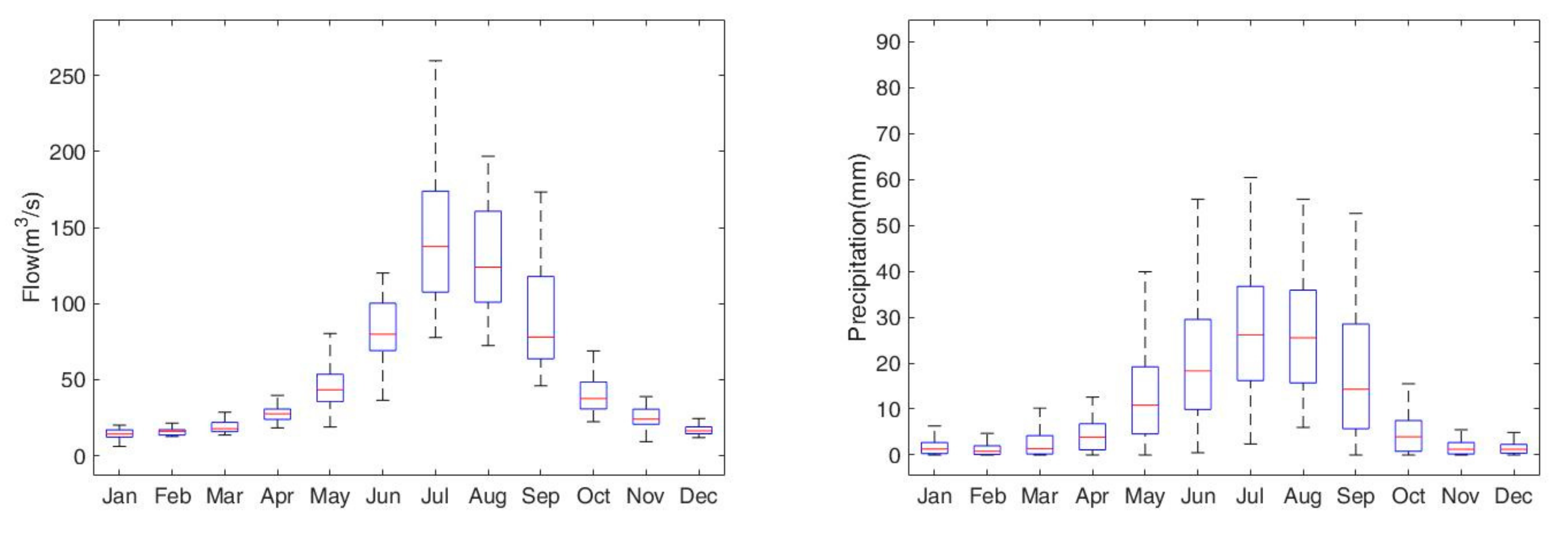
The distribution of monthly runoff and precipitation is shown in the Figure 2. It can be seen that the randomness of rainfall and runoff from June to September is much higher than that of other periods. The average price of wheat, corn and cotton was $0.33, $0.31 and $1.39, respectively. The standard deviations of prices are $0.025, $0.024 and $0.26, respectively. The price of cotton is more random than the price of wheat and corn. The stochasticity mentioned above together constitutes the source of the uncertainty of comprehensive scheduling.
The stochastic agricultural water demand was calculated by Formulas (3)–(5). The stochastic reservoir inflows and water requirements were used as the inputs of the optimal operation model. The sustainable boundaries calculated in Section 2.2 were used as the boundary conditions of the optimal operation model. The water supply of the reservoir at each time period was taken as decision variables. Minimizing the economic losses is taken as the objective function. The mathematical expression of the model is written as Formula (12):
where is the water supply of the reservoir to crop j during t period (m3), is the water supply of the reservoir to industrial during t period (m3), is the water supply of the reservoir to urban life during t period (m3), is the water supply of the reservoir to ecosystem during t period (m3), AW(t) is the available water at time T of the reservoir and SBlow and SBup are the upper and lower limits of the sustainable boundaries (m3/s).
The model was solved by the decomposition coordination algorithm and adaptive genetic algorithm [31]. For each set of solutions calculated, the water supply, storage and corresponding economic losses of the reservoir in each period were recorded. When the economic loss is below the set threshold of economic losses, the economic goal is achieved (); otherwise, the economic goal is not achieved (). When the ecological discharge of the reservoir is located within the sustainable boundary during the operation period, the ecological target is achieved (); otherwise, the ecological target is not achieved (). The mathematical expression is written as follows:
where U is the state values of ecological or economic target, Vmax is the economic benefits of crops without water stress and Vthreshold is the economic loss threshold.
The calculated results of the model will be used as learning samples to train the DBN model.
2.4. Establishment of the DBN Model
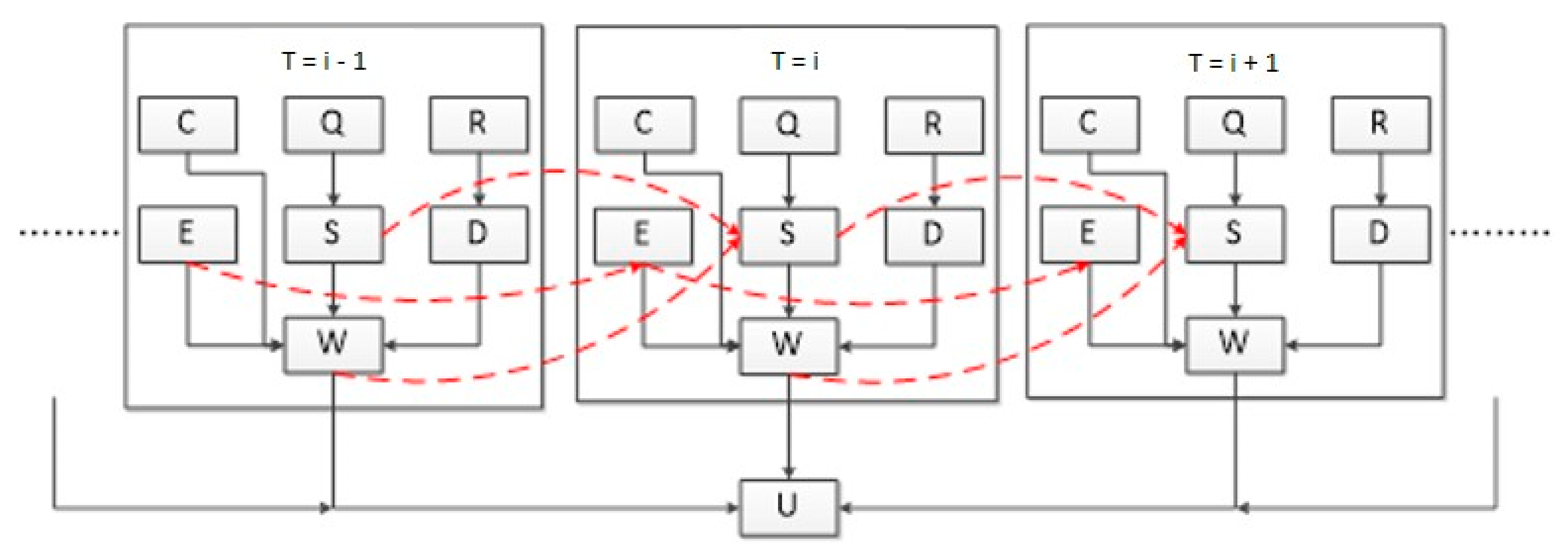
DBN is comprised of multiple static BNs and transfer networks between static BNs [14]. It combines the static BNs with the time information to form a new stochastic model for processing time-series data. In this work, the node and network structure of BNs are determined by domain expert knowledge and the network parameters are learned from the learning samples by machine learning method. The DBN model generally consists of the following four steps:
- (1)
- Select variables. A set of variables that changes over time is taken to represent certain discrete physical data values. To simplify the model, the following parameters of scheduling model are selected: inflow, rainfall, storage of the reservoir, water demand, ecological status, water supply, crop prices and state of objective, which constitute a set of variables affecting the reservoir operation status {Q, R, S, D, E, W, P, U}.
- (2)
- Determination of the causality. The reservoir operation process is described as a causal network among nodes and is a causal relationship between the inflow, rainfall and reservoir water supply. It consists of three parts: the first part is the causal relationship between rainfall and water demand; the second part is the causal relationship between reservoir inflow and storage; the third part is the causal network between water demand, reservoir storage, ecological status and reservoir water supply.
- (3)
- Time spreading. To grasp the time variability of reservoir operation uncertainty, each BN is supplemented with additional nodes for continuous time periods. These additional nodes are only related to the BN in the previous or next time period and have nothing to do with other networks. In this work, the reservoir storage, ecological status and reservoir water supply are used as additional nodes, according to expert knowledge. The ecological state at t has impact on the ecological state at t + 1. Furthermore, the reservoir storage and reservoir water supply at t have impact on the reservoir storage at t + 1.
- (4)
- Parameter learning. The prior probability distributions and the conditional probability distribution tables (CPTs) of the nodes in DBNs are learned from the learning samples achieved in the optimal operation model. However, the lack of data often occurs in real situations. To deal with the incomplete learning samples, the expectation maximization (EM) algorithm [32] is used for the parameter learning in this work, which is largely a kind of maximum likelihood estimation. The mathematical expression of the log-likelihood L(θ|X) function is:where X is the observed samples, Z is the latent variable, θ is the model parameter and P(X, Z|θ) is the marginal probability density function.
In order to solve Formula (11), first the EM algorithm sets the initial value θ0 and then executes the following iteration until it converges.
Expectation step: The function Q(θ|θt) is solved, as shown below. The expectation of latent variable is calculated, based on the model parameters of the last iteration (or initial value) to serve as the present estimate of latent variable, as follows:
where θt is the value of θ in the tth iteration and is the likelihood function’s expectation of Z.
Maximization step: The parameter θi+1 is calculated through maximizing the likelihood function based on the observed samples. The mathematical expression is
The converged parameters are stored in the CPTs of the DBN.
2.5. Decision Support Based on Uncertainty Analysis
The trained DBN can quantify the uncertainty during the process of reservoir operation by calculating the joint probability distribution function of each objective. Furthermore, the water drawing of the reservoir can be adjusted dynamically by the acceptance of uncertainty to the decision-makers.
2.5.1. Uncertainty Estimation
The Bayes rule (Formula (17)) was used to calculate the posterior probabilities of the nodes in DBN’s conditional upon evidence:
where X is the stochastic variable, e is the evidence, P(X|e) is the posterior probability of X, is the standard likelihood and P(X) is the prior probability of X.
In this work, the EM algorithm is used for uncertainty inference, and it can also help us to make the probability inference in the case of missing partial data.
2.5.2. Trade-Off Analysis
In this work, authors mainly consider the influence of water supply on economic loss objective and ecological objective. The establishment of economic loss objective needs to be combined with the economic development of the research area and adapt to the ecological objective. The influence of different water supply operations on the uncertainty of economic loss objective and ecological objective can be quantitatively analyzed by the DBN. Typically, the economic benefit decreases with the increasing of water supply over a period of time. In addition, the ecological benefit decreases with the increasing of consumable water supply (as shown in Figure 3a). Therefore, the exchange ratio between the uncertainty of unacceptable economic loss and the uncertainty of unacceptable ecological benefit destruction can be calculated using Figure 3a. The recommended water supply was determined by the expected exchange ratio algorithm (Figure 3b). The expected exchange ratio algorithm [33] obtains the recommended supplying water by providing a desired exchange ratio to the decision-makers. Since similar economic and ecological objectives were selected, the expected exchange ratio was selected as 1 in this study. If there were no point with an exchange ratio of 1, the solution with the exchange ratio closest to 1 will be selected.
3. Study Area
3.1. Description of the Study Area
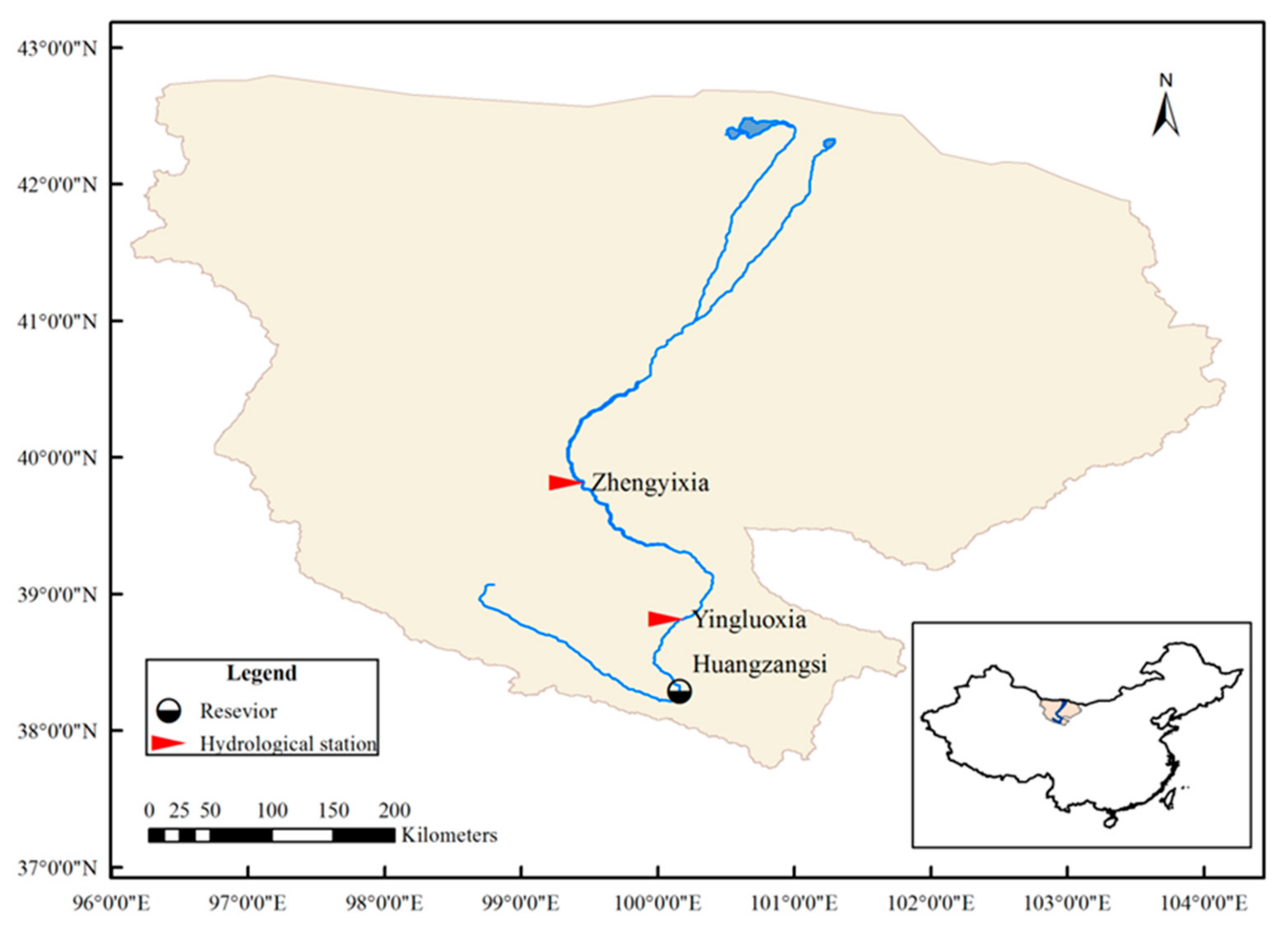
The study area is located in the middle reaches of the Heihe River in China, as shown in Figure 4. The Heihe River is the second largest inland river in northwest China, lying between Yingluoxia and Zhengyixia, with a length of 185 km and spanning an area of 25,600 km2. The basin has a long history of agricultural production, with mainly crops planted, including wheat and corn. Here is the major grain-producing area in the Gansu Province. The annual precipitation in this region is only 140 mm, but the annual evaporation is as high as 1410 mm, which makes it an area with extreme water shortage [34]. Owing to the lack of large regulation and storage project in the mainstream Heihe River, the annual runoff from the river often cannot meet the water demand for irrigation in the irrigation period.
The State Council of China approved the construction of the Huangzangsi key water-control project across the Heihe River, aiming to rationally allocate the ecological and social water resources in the middle and lower reaches, so as to improve the comprehensive management capacity of water resources. The Huangzangsi key water-control project, 11 km below the intersection of the east and west of the upper reaches of the Heihe River, was initiated in 2016 and is expected to be completed in 2021. The reservoir has a total storage capacity of 403 million cubic meters (m3), a normal dead storage capacity of 61 million cubic meters and a utilizable capacity of 334 million cubic meters. One of the challenges of the Huangzangsi Reservoir operation is to meet the social and economic water demand without damaging the hydrological regime of the river.
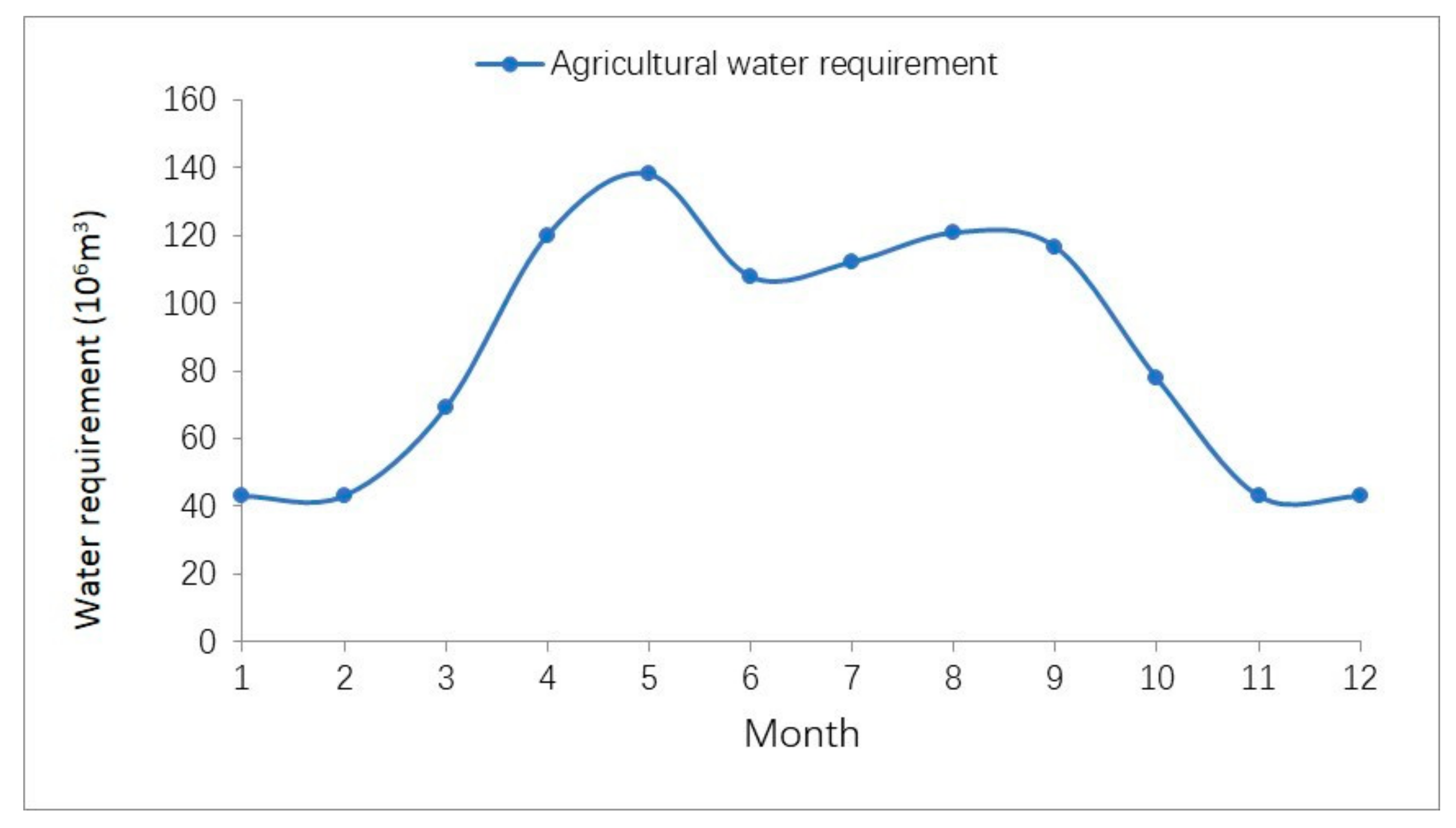
In this work, the daily runoff data of Yingluoxia and Zhengyixia were obtained from the data set of estimation on channel section flow and stage in the middle reaches of the Heihe River Basin [35], the data of rainfall were obtained from the Hydrological Yearbook of the People’s Republic of China [36], and that of urban water demand were obtained from the Data Management Center of Heihe Project (http://heihe.tpdc.ac.cn/zh-hans/ (accessed on 1 December 2019)) [7]. Moreover, the data of irrigation quota and irrigation area of each crop were obtained from the research on rational allocation and carrying capacity of water resources in the northwest China and also provided by the Heihe Watershed Authority [37]. Furthermore, the data of evaporation in the Heihe River Basin were from the Data Management Center of Heihe Project [38]. The main crops in the study area are wheat, maize and cotton. Data on grain production and agricultural prices in the study area were obtained from the National data web site (http://data.stats.gov.cn (accessed on 1 December 2019)). The crop yield response factor and the crop coefficient were obtained from the Main Crop Water Requirement and Irrigation of China [39]. Table 1 presents the crop yield response factor (ky) and crop coefficient (kc) of the main crops in different growth periods. Figure 5 shows, after calculation, the process of agricultural water requirement under 50% precipitation frequency.
3.2. Establishment of the Model
First, the natural daily runoff data of Yingluoxia from 1979 to 1999 were taken as a reference sequence. The dispatching simulation period of optimal operation model is from 2000 to 2014. In this study, the sustainable boundary was formulated by setting the combined parameters of allowable deviation from natural conditions in flood and non-flood seasons, and on that basis, an optimization model was set up for solution with a genetic algorithm, to gain the parameter combination. To prevent the hydrological regime of river being damaged by reservoir operation, the objective function is to obtain the deviation of simulative flow from the reference sequence. Furthermore, the requirement of the 97 Water Diversion Scheme for Ecological Flow in Zhengyixia is taken as the constraint condition.
Second, an optimal operation model of the Huangzangsi Reservoir was established in accordance with Section 2.3, with the inflow and rainfall of the Huangzangsi Reservoir from 2000 to 2014, which were generated by the Monte Carlo simulation, as the input of the model, and the sustainable boundaries and water requirement as the boundary conditions of the model. Then a DBN model was established in detail in Section 2.4. Figure 6 shows the specific conditional independence and dependence relations among the nodes of DBNs.
Table 2 shows the nodes of the DBN model. The value range of the nodes is determined by the maximum and minimum values of the measured data. Each node is uniformly discretized based on the frequency distribution and the number of states. The CPTs are learned by the results of the optimal operation model of Huangzangsi Reservoir.
Finally, the trained DBN model can be used to infer the uncertainty and provide guidance for the operation of Huangzangsi Reservoir.
4. Result and Discussion
4.1. Determination of Sustainable Boundaries
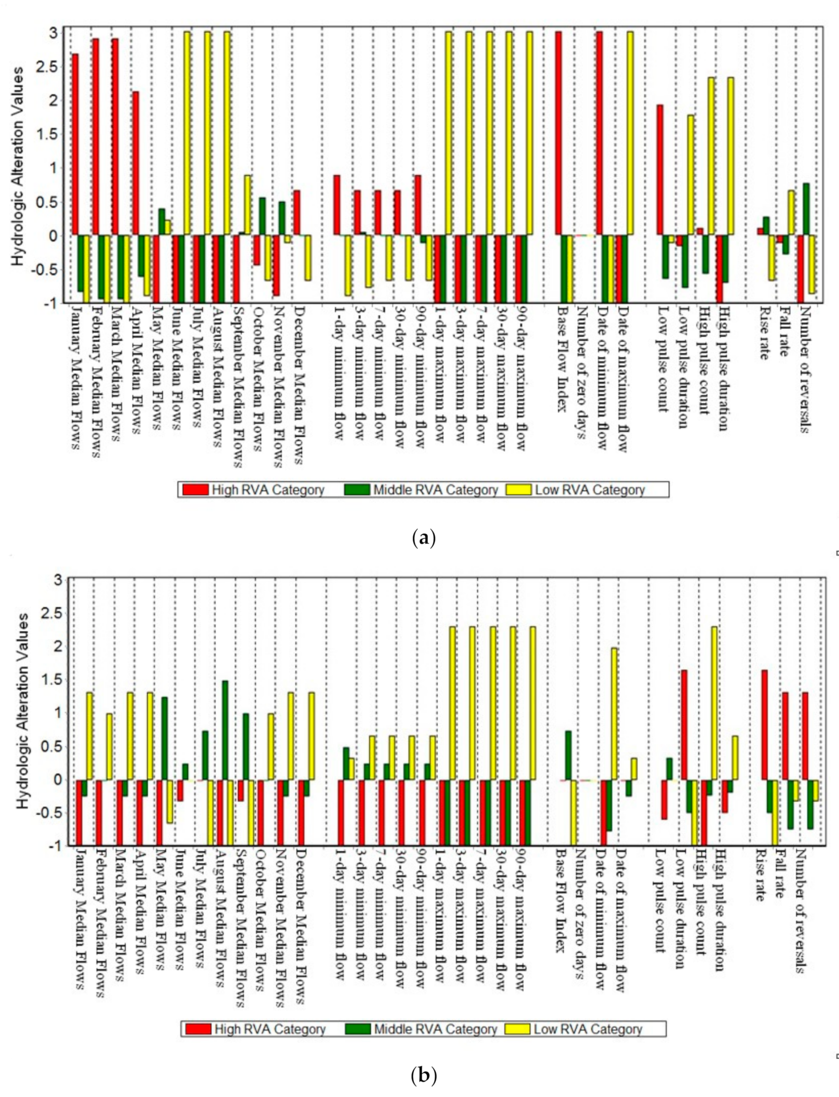
The reservoir operation was simulated for different boundaries, and its respective hydrologic alteration was calculated, to study the protection of SBA for river hydrological regime. Moreover, the requirements of the 97 water diversion scheme for ecological flow and water supply in Zhengyixia were considered as the constraints. As shown in Figure 7, when compared with the current situation of the study area, the comprehensive hydrologic alteration under the constraint of ecological flow sustainable boundaries decreases from 79% to 62%. Among them, the hydrologic alteration degree of monthly flow magnitude index decreases from 70% to 52%. However, due to the constraint of sustainable boundaries, the flow from May to September tends to be flat. The alteration degree of the annual extreme flow magnitude and duration index increases from 51% to 60%, indicating that the protection provided by the sustainable boundaries to this group of indicators is relatively limited. From the perspective of the frequency and duration of high pulse flow, the alteration degree of this group of indicators is reduced from 67% to 31%. It can be seen that the sustainable boundary of ecological flow is relatively effective for the protection of high and low pulse flow. The results show that the sustainable boundary of ecological flow established in this section reduces the comprehensive hydrologic alteration. It is more effective in protecting the magnitude index of monthly flow and the frequency and duration index of high pulse flow, but it has only limited effect in reducing the alteration of the other three groups of indices. Figure 8 shows the optimized sustainable boundary.
4.2. Dynamic Regulation in Different Time Steps
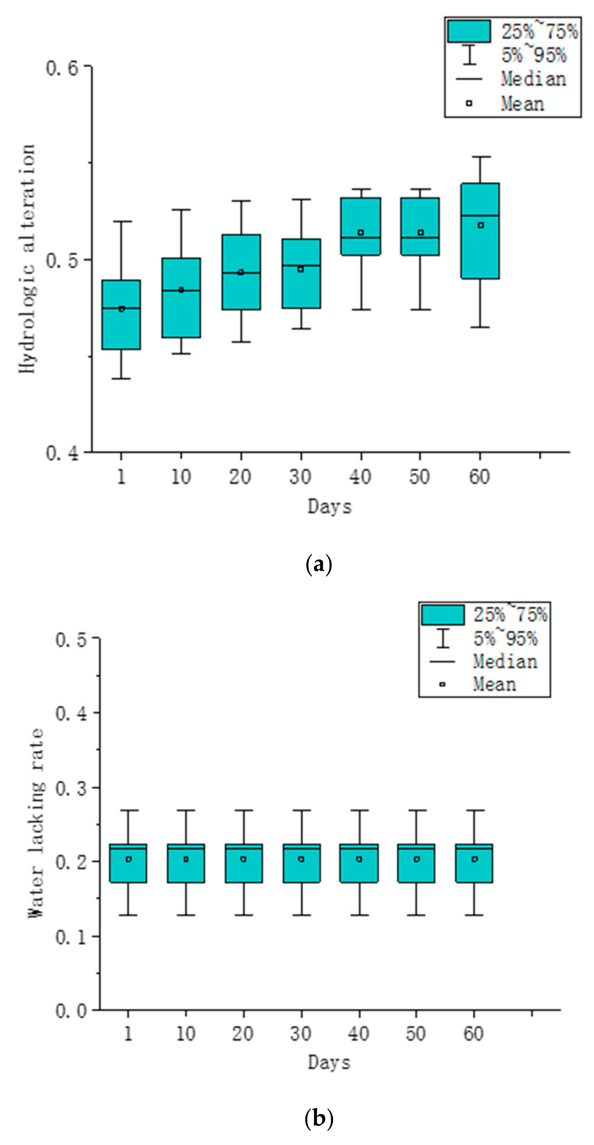
The selection of time scale is very important for the dynamic adjustment of reservoir operation. In the reservoir operation model, the hydrologic alteration and the water supply reliability increase with the increasing time step under the constraint of reservoir operating rule curves [40]. To analyze the effect of time step on reservoir operation under the constraint of sustainable boundary, 10 groups of runoff data are generated by the autoregressive model. The optimization model (established in Section 2.3) is used to simulate the optimal reservoir operation and calculate the hydrologic alteration and the water shortage rate. In this section, the impact of the dynamically-adjusted time steps on reservoir operation was analyzed. Thus, to eliminate the influence of flow simulation at different time scales on hydrologic alteration, the calculated results of each time step were decomposed into daily flow under the constraint of sustainable boundaries.
As shown in Figure 9a, for a slight increase of hydrologic alterations, the mean and median values of hydrologic alterations change a little in different time steps, because the sustainable boundaries measured on a daily scale provide adequate protection for river flow regime. The mean and distribution of water lacking rates are almost unchanged, as shown in Figure 9b. The sustainable boundary which is calculated in Section 2.2 can provide guidance on the determination of water quantity and flow regime for reservoir operation. Therefore, considering the difficulty of calculation, 30–60 days can be selected as the time step of dynamic adjustment under the constraint of sustainable boundaries. To match with the agricultural water demand data, 1 month (30 days) is used as the time scale of the decision support model in this work.
4.3. Uncertainty Analysis of Reservoir Discharge Operation
According to the reference [41], the median willingness to pay for restoring the ecology of the Ejina watershed from the referendum formats was about 8% of the resident income. Therefore, keeping the flow within the sustainable boundaries and the agricultural loss within 8% of agricultural income without water stress, respectively, were selected as the ecological and economic objectives of uncertainty analysis.
To analyze the effect of different water supply on the uncertainty of reservoir operation targets, in this study, the uncertainty of economic and ecological targets was calculated by taking the proportion of water supply as the evidence node, and the probability of the target exceeding the set threshold was taken as the uncertainty of the target. The uncertainty of economic target is written as:
The uncertainty of the ecological target is expressed as:
where, U is the state values of the operation targets, W/Wmax is the proportion of water supply, and P is the probability of the state value of the operation target equal to 0 when the proportion of water supply is taken as the evidence node.
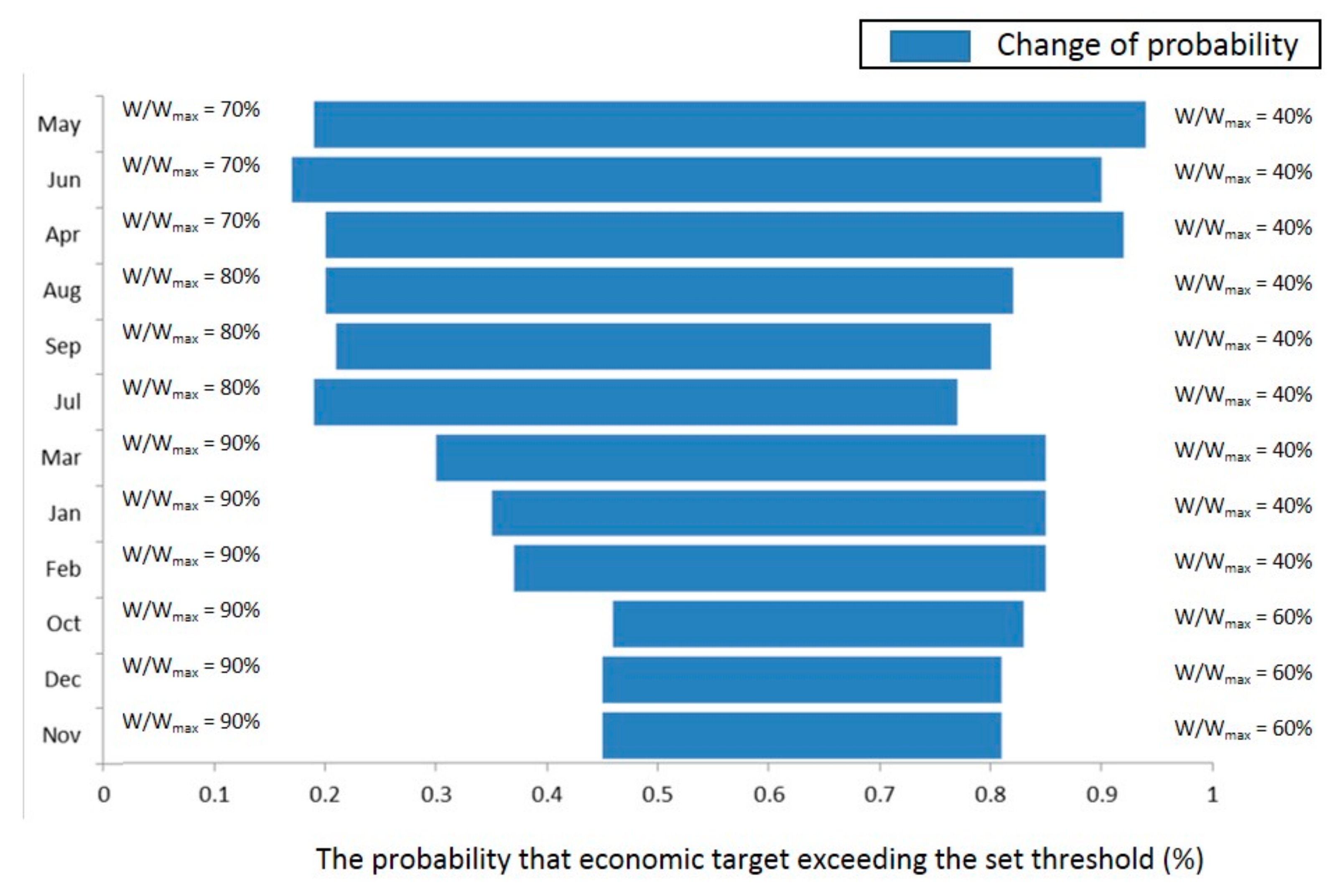
In this study, AgenaRisk software (https://www.agenarisk.com (accessed on 1 December 2019)) was used for the sensitivity analysis of water supply proportion in each month by taking the probability of the economic target exceeding the set threshold as the target. In the tornado graph, the length of the bars for each sensitivity variable is a measure of the influence of that variable on the target variable (Figure 10). The abscissa represents the probability of the economic target exceeding the set threshold, and the ordinate represents the time period. The left and right marks represent the proportion of water supply. Figure 10 shows that the proportions of water supply in May, June and April have the greatest impact on the target variable. When the proportion of water supply increases from 40% to 70% in May, the probability of the economic target exceeding the set threshold decreases from 94% to 19%. The proportions of water supply in November, December and October have least impact on the probability of the economic target exceeding the set threshold. When the proportion of water supply increases from 60% to 90% between October and December, the probability of the economic target exceeding the set threshold only decreases by about 36%.
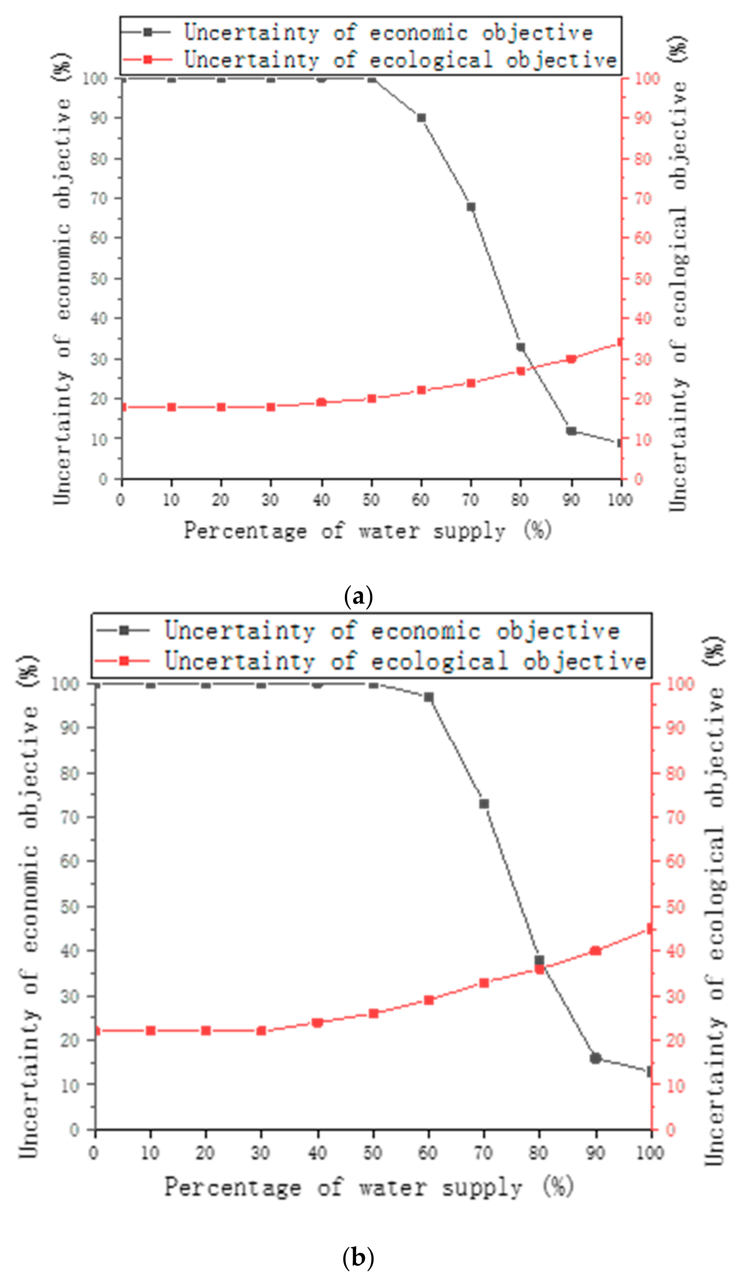
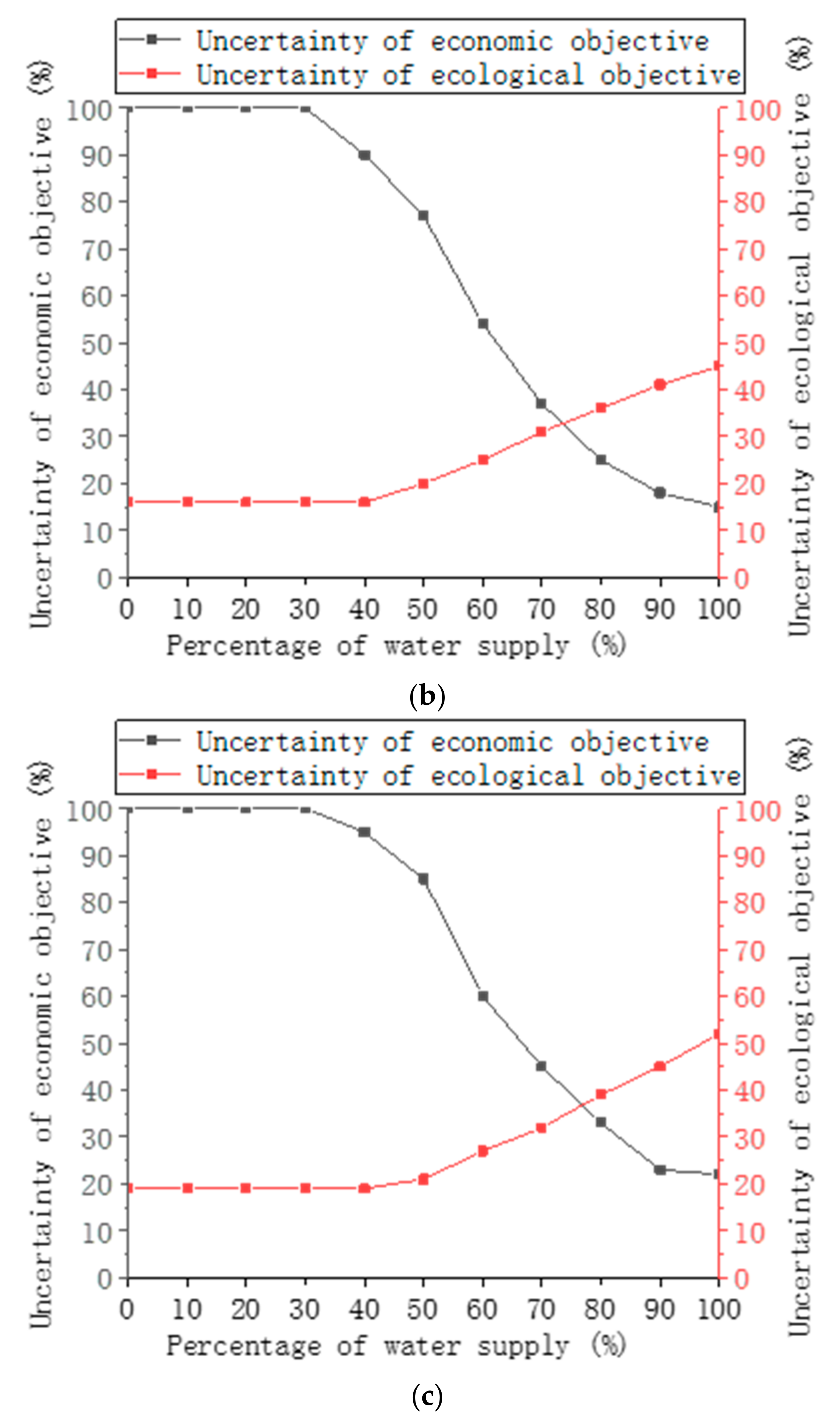
To analyze the change in reservoir operation uncertainties during different time periods in different typical years, May and September, the starting and ending of agricultural water peak, were selected as examples for this study, to reveal the response of the probability of operation target exceeding the set threshold to the percentage of water supply. Herein, the operation of the reservoir was simulated, and the previous water supply was set as the evidence node. The water supply proportion in May and September was set as 0 and 100%, respectively, to observe the probabilities of operation targets exceeding the set threshold. Figure 11a–c shows the impact of different water supply choices on the uncertainty of economic and ecological objectives in May of wet, normal-flow and low-flow year, respectively, and the inflow frequency of the wet, normal-flow and low-flow year (1983, 1989 and 2002 were selected as the typical years, respectively) are 25%, 50% and 75%, respectively. The main irrigated crops of the study area in May are wheat and cotton. The crop response coefficient of wheat is higher than that of cotton. After completion of wheat irrigation, the value of irrigation water per unit will decrease. Thus, with an increase in water supply, the rate at which the uncertainty of economic objective decreases first increases and then decreases. As shown in Figure 11, the increase in the water supply increases the uncertainty of ecological objective gently.
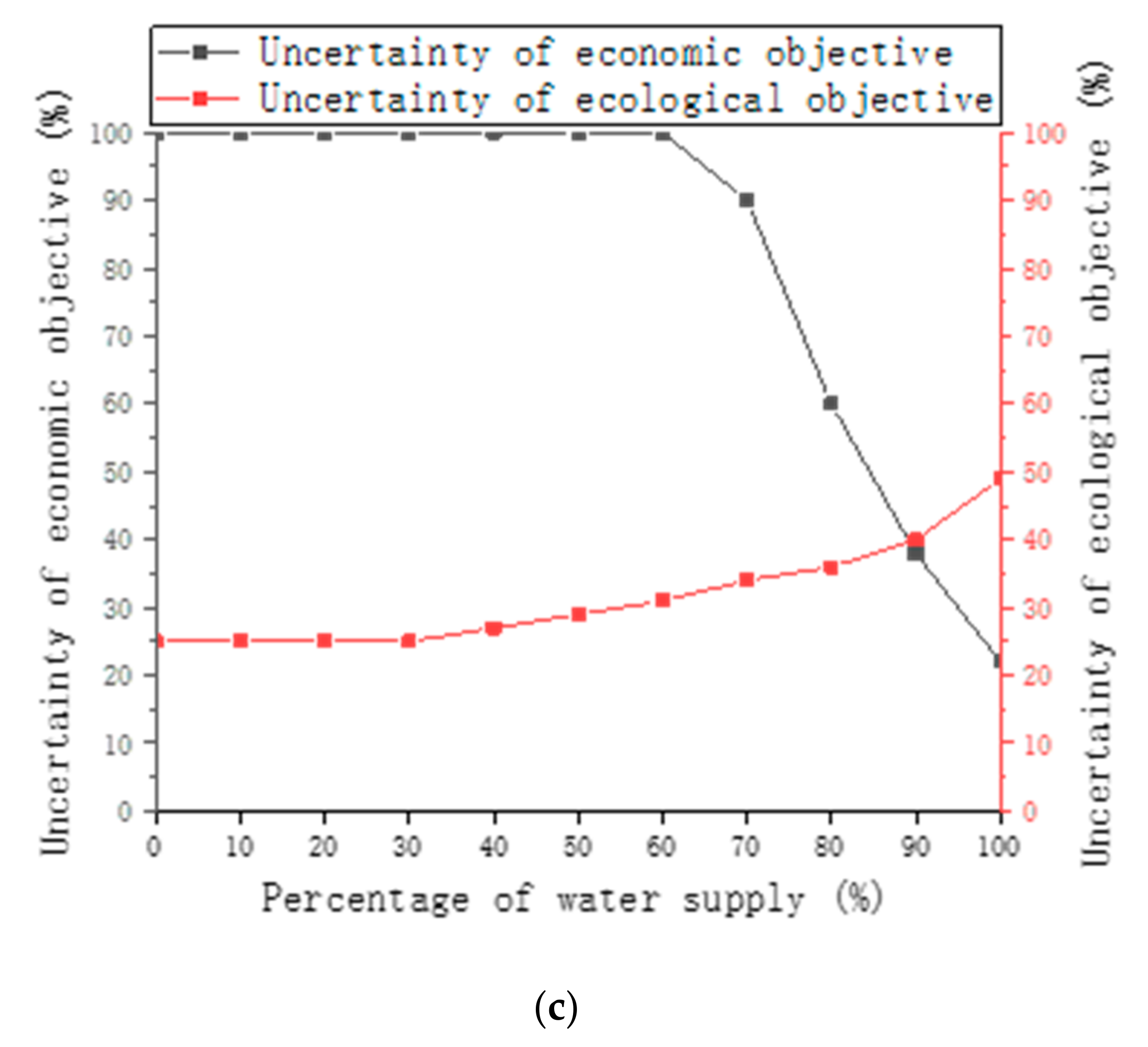
Figure 12a–c shows the impact of different water supply choices on the uncertainty of economic and ecological objectives in September of the wet, normal-flow and low-flow years, respectively. It can be inferred from the figure that the benefits of increasing agricultural water supply to reduce the uncertainty of economic objectives begin to decrease after 70% of agricultural water needs are met. This is because the period with the greatest impact on crop yields (April and May) is over. At this stage, ecological drainage can be appropriately increased once 60% of the agricultural water supply has been completed.
4.4. Analysis of Model Effectiveness
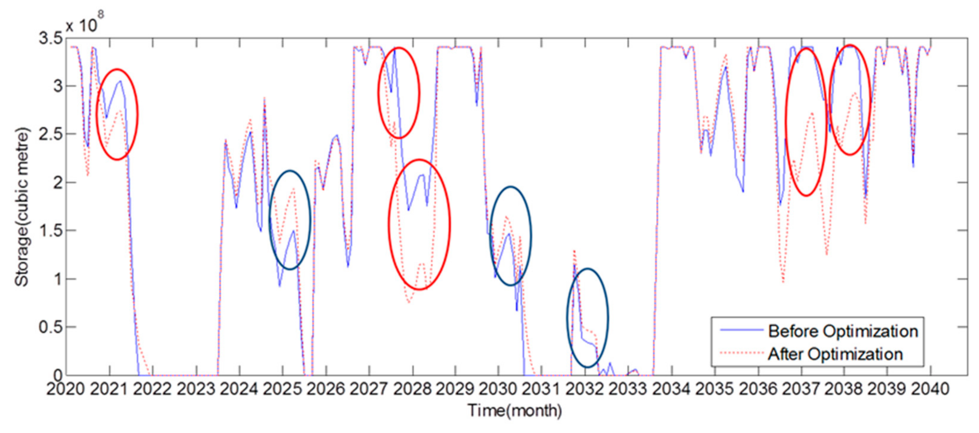
To verify the validity of the decision support model, a group of 20-year monthly flow was generated through Monte Carlo simulation based on the 20-year natural monthly flow of Huangzangsi as the input to the model. Figure 13 shows the changes of water storage in the reservoir under two different operation modes with the same reservoir inflow. The first one is based on the designed guaranteed rate, which is also the current operation mode in the study area. That is, the normal agricultural water supply is adopted when the inflow frequency is lower than the designed guaranteed rate, while the restricted agricultural water supply is adopted when the inflow frequency is higher than the designed guaranteed rate. The limit coefficient of agricultural water supply is 0.7. The change of reservoir storage in this mode is represented by the solid blue line. The second mode is the proposed operation model, which determines the proportion of agricultural water supply in the current period based on the probability of the current ecological and economic goals exceeding the set threshold. The change of reservoir storage in this mode is represented by the red dotted line. In Figure 13, the red circle indicates the increased water supply by the proposed operation mode, whereas the blue circle indicates the decreased water supply by the DSS mode. The increased water supply occurs mostly when the reservoir storage is above 150 million cubic meters, while the decreased water supply and the increased water storage mostly occur when the reservoir storage volume is less than 150 million cubic meters. In general, the water supply strategy based on the designed guaranteed rate is relatively conservative. In normal years, the decision support model increases the proportion of agricultural water supply. In addition, there is little difference between the two modes in extremely abundant years and extremely dry years.
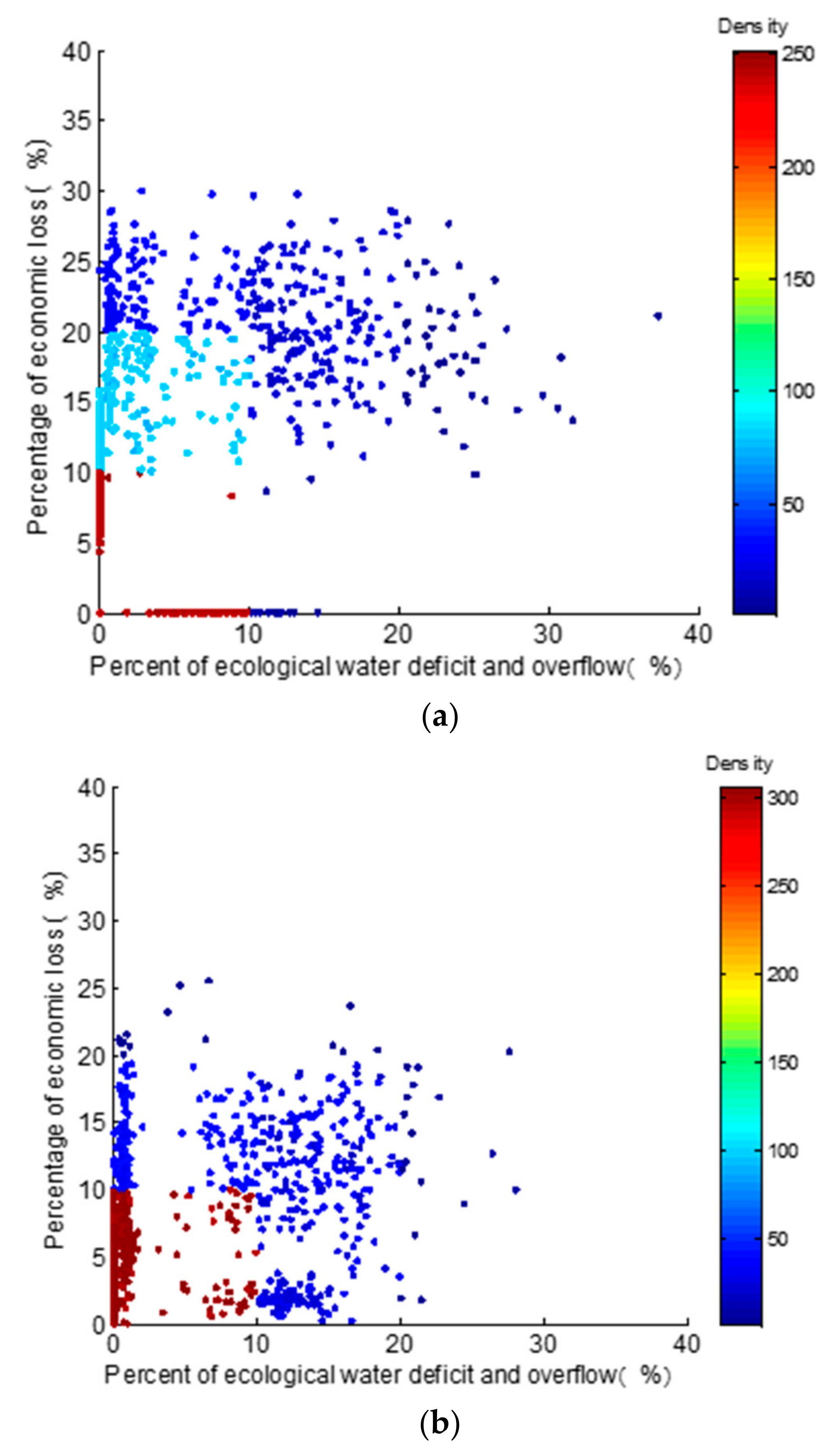
In order to study the effects of the two operation modes and the performance of dealing with uncertainties, 99 groups of 20-year monthly flow, rainfall and crop prices sequences were generated by taking the measured data as samples in this paper. These data were used as inputs of the operation model based on the designed guaranteed rate and the operation model considering uncertainties respectively. In this paper, the ecological flow shortage rate, the overflow rate and economic loss rate were used to evaluate the ecological and economic benefits of each reservoir operation scheme. The rate of ecological flow shortage and overflow refers to the proportion of the ecological flow beyond the sustainable boundaries in the total ecological flow. Economic loss rate refers to the proportion of the economic loss caused by water stress in the total economic output of crops. Figure 14 shows the annual ecological flow shortage rate, the overflow rate and the economic loss rate of 100 groups of 20-year flow series under two different reservoir operation models. The horizontal and vertical coordinates of each data point in the figure represent the ecological overflow rate, the water shortage rate and the economic loss rate of the year, respectively. The color of each point represents the density of results distribution. The results show that, when the operation model based on the designed guaranteed rate is adopted, the main variation range of the economic loss rate is 0–28% and the main variation range of the ecological overflow and water shortage rate is 0–25%. When the decision support model based on DBN is adopted, the main variation range of the economic loss rate is 0–22% and the main variation range of the ecological overflow water shortage rate is 0–20%. Compared with the operation model based on the designed guaranteed rate, the decision support model based on DBN can reduce the variation range of the ecological flow shortage and overflow rate and the economic loss rate by 5% and 6%, respectively. It can be seen that the model proposed in this paper can effectively exert the regulating capacity of reservoir and reduce the influence of inflow and rainfall uncertainties on reservoir operation.
Some scholars [17,18,19] calculated the recommended ecological flow with the Bayesian network model to guide reservoir operation. However, the recommended ecological flow rule is same as the 97 water diversion scheme, which is a static reservoir operation rule. The static reservoir dispatching rule has two defects, including its failure to take the condition changes of the reservoir (such as reservoir storage) into account, and its failure to account for the uncertainty changes of reservoir operation. For example, the probability of economic losses exceeding a set threshold in a dry year increases over time, and vice versa in a wet year. The model proposed in this paper can give a scientific recommended water supply by comprehensively considering these two points. Figure 11, Figure 12 and Figure 14 illustrate the advantages of dynamic operation in reducing the uncertainty of reservoir operation compared with the static rules. Considering the time-varying characteristics of flood risk, some scholars have established the dynamic control model of single objective for reservoir flood control [14]. On this basis, the particularity of the calculation economic objective, and the coordination between the objectives of ecological and social economic benefits were further taken into consideration in the proposed model.
At the same time, compared with the recommended ecological flow rules, the disadvantages of the proposed model are also very obvious. It is difficult to collect data and establish the model of agricultural economic loss in an economically undeveloped area. Adjusting the reservoir operation strategy based on real-time information will also increase the operation cost of the reservoir. So, reservoir management has to consider the balance between science and practicality. The advantage of reservoir dynamic adjustment strategy is obvious if there is sufficient data support and fund guarantee. However, if such conditions are not available, the static reservoir operation rules are more efficient. Therefore, according to the calculation results of the model, the recommended water storage of the reservoir in different periods at different risk levels is proposed as a simple guide for reservoir operation in Section 4.5.
4.5. Response Analysis of Target Uncertainty to Reservoir Storage Available
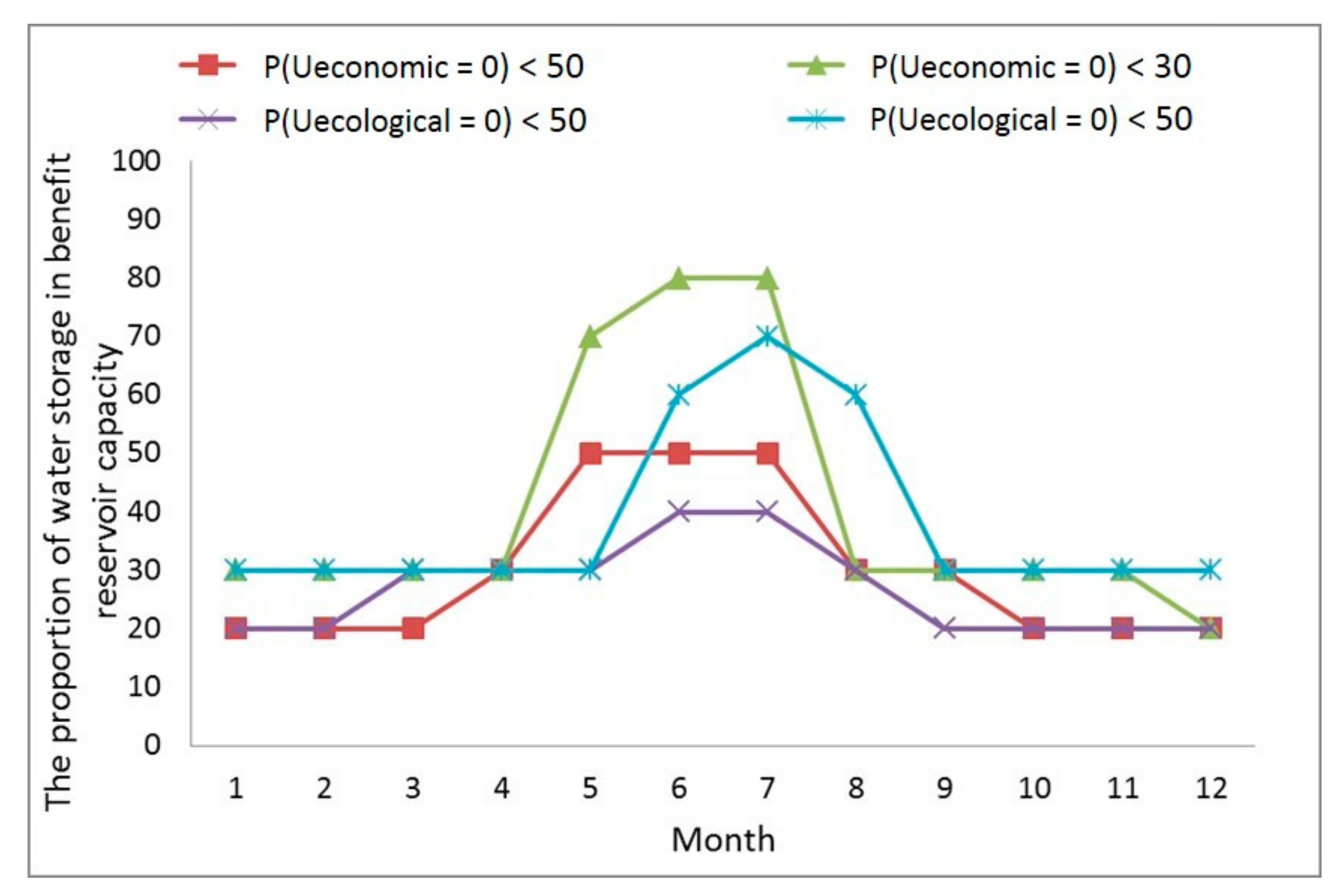
The water available in a reservoir has a great influence on the uncertainty of economic and ecological objectives. At the same time, the reservoir water level (storage) is also an important indicator of reservoir operation. Therefore, in this study, the water supply was set as the hidden node, the time extension was cancelled and the EM algorithm was used to separately calculate the impact of the reservoir water storage on the uncertainty of economic and ecological goals in each period. To provide guidance for reservoir operation, the amount of water available to be maintained in different periods of time to meet the different requirements of uncertainty was also calculated in this study (as shown in Figure 15).
Figure 15 shows the reservoir water storage requirements that keep the uncertainty of the economic and ecological targets below 50% and 30% in different periods, respectively. From the timeline, the water storage demand curve of the reservoir shows its peak in the middle and its valley on both sides. After July, the uncertainty of the economic target reduces the demand for water storage in the reservoir rapidly. This is because most of the water supply is completed by July. After September, the ecological requirement for the reservoir storage is reduced to 20–30%. From the point of view for different uncertainty levels, maintaining a lower uncertainty level requires the reservoir water storage to have a greater fluctuation trend, and so the reservoir should maintain a higher amount of available water resources during the flood season. However, it is difficult to keep the reservoirs running at high water levels in dry areas. Therefore, it is reasonable to keep the uncertainty of economic and ecological targets below 30%. Thus, the reservoir should hold 70–80% of beneficial reservoir capacity from June to August (i.e., 230–260 million cubic meters of available water). Authors think this can provide some guidance for the formulation of reservoir operation chart.
In this study, a decision support model was proposed to calculate the uncertainties of economic and ecological targets by establishing optimization operation model and DBNs model. Compared to the previous research studies, the proposed model allows decision-makers to adjust the reservoir operation according to the acceptance of risk and the current states and describes the flow management process in more detail (instead of only the overall ecological goal). At the same time, decision-makers can formulate operation rules (such as the reservoir operation chart) for the reservoir according to the acceptance of risk.
5. Conclusions
To coordinate the socioeconomic and ecological environment competition for water-scarce resources in arid areas, a decision support model with four parts was established in this study and the proposed model was applied herein to the middle reaches of the Heihe watershed to formulate the sustainable boundaries, with the IHA as the standard. Based on the existing research, the time-varying characteristics of the uncertainty of reservoir operation, the particularity of the calculation of social and economic objective, and the coordination between the objectives of ecological and social economic benefits were taken into consideration in the proposed model. The results show that the optimized sustainable boundary can reduce the hydrologic alteration of the study area from 79% to 62%. The optimal operation model generated the learning cases and calculated the economic losses of each case, while the DBN model was established and trained by learning examples. The trained DBN model can be used for uncertainty inference. The expected exchange ratio provided by the decision-maker can be used to coordinate water conflicts of ecological and economic objectives. The main conclusions of this research are as follows:
Firstly, this study shows through calculation that the proportions of water supply in May, June and April have the greatest impact on the probability of the economic target exceeding the set threshold, whereas those in November, December and October have the least impact on the probability of the economic target exceeding the set threshold. According to the further analyses, the ecological drainage or storage can be appropriately increased after 70% of the agricultural water supply has been completed in September. Then, by simulating and analyzing the operation process of the Huangzangsi Reservoir with the model based on the designed guaranteed rate and the model considering the uncertainty, it is found that the current designed guaranteed rate in the study area is relatively conservative, and the decision support model considering uncertainty in normal years tends to moderately increase the proportion of agricultural water supply. To measure the performance of the two operation models in dealing with the uncertainty, 100 groups of 20 years of data for monthly flow, rainfall and crop prices were generated as the model inputs to simulate the reservoir operation. The results show that the decision support model based on DBN reduces the variation range of the ecological flow shortage and overflow rate and the economic loss rate by 5% and 6%, respectively. Obviously, the model proposed in this study can effectively exert the regulating capacity of the reservoir and reduce the effect of inflow and rainfall uncertainties on reservoir operation. At last, reserving 230–260 million cubic meters of water in the reservoir between June and August could reduce the uncertainty of economic and ecological objectives below 30%. Additionally, it is recommended to take all these factors into account for formulation of the reservoir operation chart.
In the results and discussion section, the advantages and disadvantages of the proposed model and the recommended ecological flow rules were discussed. The advantage of reservoir dynamic adjustment strategy is obvious with sufficient data support and fund guarantee. However, if such conditions were not available, the static reservoir operation rules would be more efficient. In addition, the formulation of reasonable ecological and social economic objectives was important basis for the proposed model to make scientific decisions. In this study, the economic objective that matches the ecological objective was established on the basis of the research on the willingness to pay for environmental restoration in the Heihe River Basin [41]. However, with the change of the exchange ratio of ecological environment and economic benefits, the willingness to pay of people will also change. Therefore, during the actual operation of the reservoir, the social and economic objectives matching with different ecological and environmental protection degrees should be taken into consideration. In addition, it is a complex socio-hydrology problem.
Author Contributions
This study was designed by T.Z. and Z.D., and the first draft of the manuscript was written by T.Z. Then, the manuscript was organized, revised and finally edited by X.C. and Q.R. All authors have read and agreed to the published version of the manuscript.
Funding
This study was financially supported by the National Natural Science Foundation of China (Grant No. 52009005, 51779013), National Key Research and Development Program of China (2018YFC1508200), the Postgraduate Research and Practice Innovation Program of Jiangsu Prov-ince (KYCX18-0574), the Fundamental Research Funds for the Central Universities (2018B603X14) and the National Key Research and Development Program (2016YFC0401306).
Institutional Review Board Statement
Not applicable.
Informed Consent Statement
Not applicable.
Data Availability Statement
No new data were created or analyzed in this study. Data sharing is not applicable to this article.
Conflicts of Interest
Tao Zhou, Zengchuan Dong, Xiuxiu Chen and Qihua Ran declare that they have no conflict of interest.
References
- Poff, N.L.; Richter, B.D.; Arthington, A.H.; Bunn, S.E.; Naiman, R.J.; Kendy, E.; Acreman, M.; Apse, C.; Bledsoe, B.P.; Freeman, M.C.; et al. The ecological limits of hydrologic alteration (ELOHA): A new framework for developing regional environmental flow standards. Freshw. Biol. 2010, 55, 147–170. [Google Scholar] [CrossRef] [Green Version]
- Richter, B.D. Re-thinking environmental flows: From allocations and reserves to sustainability boundaries. River Res. Appl. 2009, 26, 1052–1063. [Google Scholar] [CrossRef]
- Richter, B.D.; Davis, M.M.; Apse, C.; Konrad, C. A presumptive standard for environmental flow protection. River Res. Appl. 2012, 28, 1312–1321. [Google Scholar] [CrossRef]
- Peñas, F.J.; Barquín, J. Assessment of large-scale patterns of hydrological alteration caused by dams. J. Hydrol. 2019, 572, 706–718. [Google Scholar] [CrossRef]
- De Jalón, S.G.; Del Tánago, M.G.; de Jalón, D.G. A new approach for assessing natural patterns of flow variability and hydrological alterations: The case of the Spanish rivers. J. Environ. Manag. 2019, 233, 200–210. [Google Scholar] [CrossRef] [PubMed]
- Cheng, G.; Li, X.; Zhao, W.; Xu, Z.; Feng, Q.; Xiao, S.; Xiao, H. Integrated study of the water–ecosystem–economy in the Heihe River Basin. Natl. Sci. Rev. 2014, 1, 413–428. [Google Scholar] [CrossRef] [Green Version]
- Wang, Z.; Zhu, J.; Zheng, H. Improvement of Duration-Based Water Rights Management with Optimal Water Intake On/Off Events. Water Resour. Manag. 2015, 29, 2927–2945. [Google Scholar] [CrossRef]
- Yazicigil, H.; Houck, M.H. The effects of risk and reliability on optimal reservoir design. J. Am. Water Resour. Assoc. 1984, 20, 417–424. [Google Scholar] [CrossRef]
- Pearl, J. Probabilistic Reasoning in Intelligent Systems: Networks of Plausible Inference; Morgan Kaufmann Publishers: San Mateo, CA, USA, 1988. [Google Scholar]
- Hanea, A.M.; Gheorghe, M.; Hanea, R.; Ababei, D. Non-parametric Bayesian networks for parameter estimation in reservoir simulation: A graphical take on the ensemble Kalman filter (part I). Comput. Geosci. 2013, 17, 929–949. [Google Scholar] [CrossRef]
- Castelletti, A.; Soncini-Sessa, R. Bayesian Networks and participatory modelling in water resource management. Environ. Model. Softw. 2007, 22, 1075–1088. [Google Scholar] [CrossRef]
- Morrison, R.R.; Stone, M.C. Spatially implemented Bayesian network model to assess environmental impacts of water management. Water Resour. Res. 2014, 50, 8107–8124. [Google Scholar] [CrossRef]
- Brusaferri, A.; Matteucci, M.; Portolani, P.; Vitali, A. Bayesian deep learning based method for probabilistic forecast of day-ahead electricity prices. Appl. Energy 2019, 250, 1158–1175. [Google Scholar] [CrossRef]
- Chen, J.; Zhong, P.A.; An, R.; Zhu, F.; Xu, B. Risk analysis for real-time flood control operation of a multi-reservoir system using a dynamic Bayesian network. Environ. Model. Softw. 2019, 111, 409–420. [Google Scholar] [CrossRef]
- Shin, J.Y.; Kwon, H.H.; Lee, J.H.; Kim, T.W. Probabilistic long-term hydrological drought forecast using Bayesian networks and drought propagation. Meteorol. Appl. 2019, 27, e1827. [Google Scholar] [CrossRef] [Green Version]
- Phan, T.D.; Smart, J.C.; Capon, S.J.; Hadwen, W.L.; Sahin, O. Applications of Bayesian belief networks in water resource management: A systematic review. Environ. Model. Softw. 2016, 85, 98–111. [Google Scholar] [CrossRef]
- Pang, A.; Li, C.; Sun, T.; Yang, W.; Yang, Z. Trade-Off Analysis to Determine Environmental Flows in a Highly Regulated Watershed. Sci. Rep. 2018, 8, 1–11. [Google Scholar] [CrossRef] [Green Version]
- Pang, A.P.; Sun, T. Bayesian networks for environmental flow decision-making and an application in the Yellow River estuary, China. Hydrol. Earth Syst. Sci. 2014, 18, 1641–1651. [Google Scholar] [CrossRef] [Green Version]
- Xue, J.; Gui, D.; Zhao, Y.; Lei, J.; Zeng, F.; Feng, X.; Mao, D.; Shareef, M. A decision-making framework to model environmental flow requirements in oasis areas using Bayesian networks. J. Hydrol. 2016, 540, 1209–1222. [Google Scholar] [CrossRef]
- Marcot, B.G.; Penman, T.D. Advances in Bayesian network modelling: Integration of modelling technologies. Environ. Model. Softw. 2019, 111, 386–393. [Google Scholar] [CrossRef]
- Manoj, K.; Jha, M.A. Dynamic Bayesian Network for Predicting the Likelihood of a Terrorist Attack at Critical Transportation Infrastructure Facilities. J. Infrastruct. Syst. 2009, 15, 31–39. [Google Scholar]
- Kim, S.Y.; Imoto, S.; Miyano, S. Inferring gene networks from time series microarray data using dynamic Bayesian networks. Brief. Bioinform. 2003, 4, 3228–3235. [Google Scholar] [CrossRef] [PubMed] [Green Version]
- Nefian, A.V.; Liang, L.; Pi, X.; Liu, X.; Murphy, K. Dynamic Bayesian Networks for Audio-Visual Speech Recognition. J. Appl. Signal Process. 2002, 11, 1274–1288. [Google Scholar] [CrossRef] [Green Version]
- Robinson, J.W.; Hartemink, A.J. Learning Non-Stationary Dynamic Bayesian Networks. J. Mach. Learn. Res. 2010, 11, 3647–3680. [Google Scholar]
- Richter, B.; Baumgartner, J.; Wigington, R.; Braun, D. How much water does a river need. Freshw. Biol. 1997, 37, 231–249. [Google Scholar] [CrossRef] [Green Version]
- Richter, B.D.; Baumgartner, J.V.; Powell, J.; Braun, D.P. A Method for Assessing Hydrologic Alteration within Ecosystems. Conserv. Biol. 1996, 10, 1163–1174. [Google Scholar] [CrossRef] [Green Version]
- Shiau, J.T.; Wu, F.C. Pareto-optimal solutions for environmental flow schemes incorporating the intra-annual and interannual variability of the natural flow regime. Water Resour. Res. 2007, 43, 1–12. [Google Scholar] [CrossRef]
- Zhou, T.; Dong, Z.; Wu, J.; Lin, M. Study on Joint Regulation of Fenhe Cascade Reservoirs Considering the Ecological Water Demand. Yellow River 2018, 40, 62–65. [Google Scholar]
- Tang, X.; Zhang, Z.; Wei, Y. Quantitative Evaluation of Water Resources Pressure in Heihe River Basin. Bull. Soil Water Conserv. 2014, 34, 219–224. [Google Scholar]
- Stewart, J.I.; Hagan, R.M.; Pruitt, W.O.; Danielson, R.E.; Franklin, W.T.; Hanks, R.J.; Riley, J.P.; Jackson, E.B. Optimizing Crop Production through Control of Water and Salinity Levels in the Soil. Reports. Paper 67. 1977. Available online: https://digitalcommons.usu.edu/water_rep/67 (accessed on 21 March 2021).
- Zhou, T.; Dong, Z.; Wang, W. Study on Multi-Scale Coupled Ecological Dispatching Model Based on the Decomposition-Coordination Principle. Water 2019, 11, 1443. [Google Scholar] [CrossRef] [Green Version]
- Dempster, A.P.; Laird, N.M.; Rubin, D.B. Maximum likelihood from incomplete data via the EM algorithm. J. R. Stat. Soc. 1977, 39, 1–38. [Google Scholar]
- Dong, Z. An interactive method of multi-objective decision making and its application. J. Hydraul. Eng. 1992, 4, 33–38. [Google Scholar]
- Wang, J.; Meng, J.J. Characteristics and Tendencies of Annual Runoff Variations in the Heihe River Basin during the Past 60 years. Sci. Geogr. Sin. 2008, 28, 83–88. [Google Scholar]
- Liu, S.; Xie, Z.; Zeng, Y. Estimation of streamflow in ungauged basins using a combined model of black-box model and semi-distributed model: Case study in the Yingluoxia watershed. J. Beijing Norm. Univ. Nat. Sci. 2016, 52, 393–401. [Google Scholar]
- Yellow River Conservancy Commission. Hydrological Yearbook of the People’s Republic of China; China Water & Power Press: Beijing, China, 2015. [Google Scholar]
- Hao, W. Research on Rational Allocation and Carrying Capacity of Water Resources in Northwest China; Yellow River Water Conservancy Press: Zhengzhou, China, 2003. [Google Scholar]
- Xia, T.; Wang, Z.; Zheng, H. Topography and Data Mining Based Methods for Improving Satellite Precipitation in Mountainous Areas of China. Atmosphere 2015, 8, 983–1005. [Google Scholar] [CrossRef] [Green Version]
- Chen, Y.M. Main Crop Water Requirement and Irrigation of China; Teory and Practice of Rock Mechanics Press: Beijing, China, 1995. [Google Scholar]
- Yu, C.; Yang, Z.; Cai, Y.; Sun, T. A shorter time step for eco-friendly reservoir operation does not always produce better water availability and ecosystem benefits. J. Hydrol. 2016, 540, 900–913. [Google Scholar] [CrossRef] [Green Version]
- Xu, Z.; Loomis, J.; Zhang, Z.; Hamamura, K. Evaluating the performance of different willingness to pay question formats for valuing environmental restoration in rural China. Environ. Dev. Econ. 2006, 11, 585–601. [Google Scholar]
Figure 1.
Framework of the proposed model.

Figure 2.
Analysis of stochasticity of flow and precipitation.

Figure 3.
Determination of the recommended water supply. (a) Variety of the objective uncertainty under different water supply ratio. (b) Scheme optimization based on the expected exchange ratio algorithm.
Figure 3.
Determination of the recommended water supply. (a) Variety of the objective uncertainty under different water supply ratio. (b) Scheme optimization based on the expected exchange ratio algorithm.

Figure 4.
Location of the study area.

Figure 5.
Water requirements under 50% precipitation frequency.

Figure 6.
Structure diagram of DBNs.

Figure 7.
Comparison of hydrologic alteration under different scenarios. (a) Current hydrologic alteration. (b) Hydrologic alteration under the sustainable boundary with optimized parameters.
Figure 7.
Comparison of hydrologic alteration under different scenarios. (a) Current hydrologic alteration. (b) Hydrologic alteration under the sustainable boundary with optimized parameters.

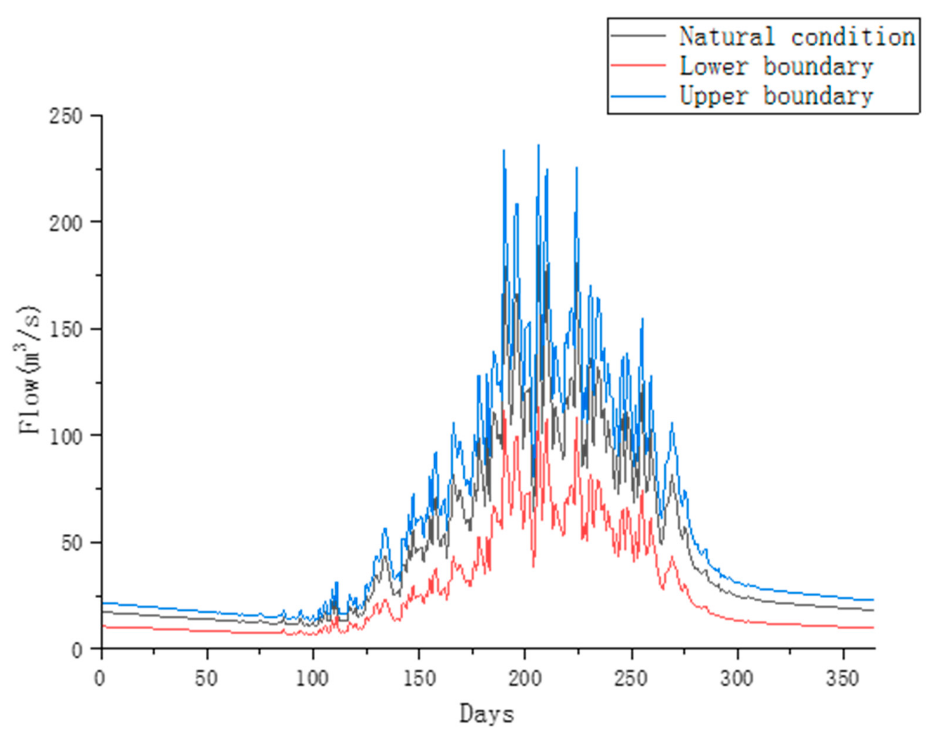
Figure 8.
Optimized sustainable boundary.

Figure 9.
Impact of time steps on reservoir operation under sustainable boundaries. (a) Hydrologic alteration in different time steps (b) Water lacking rate in different time steps.
Figure 9.
Impact of time steps on reservoir operation under sustainable boundaries. (a) Hydrologic alteration in different time steps (b) Water lacking rate in different time steps.

Figure 10.
Sensitivity analysis based on the “tornado graph” testing of the target variable “the probability of the economic target exceeding the set threshold”.
Figure 10.
Sensitivity analysis based on the “tornado graph” testing of the target variable “the probability of the economic target exceeding the set threshold”.

Figure 11.
Response of uncertainty to percentage of water supply in May. (a) Wet years. (b) Normal-flow years. (c) Low-flow years.
Figure 11.
Response of uncertainty to percentage of water supply in May. (a) Wet years. (b) Normal-flow years. (c) Low-flow years.


Figure 12.
Response of uncertainty to percentage of water supply in September. (a) Wet years. (b) Normal-flow years. (c) Low-flow years.
Figure 12.
Response of uncertainty to percentage of water supply in September. (a) Wet years. (b) Normal-flow years. (c) Low-flow years.


Figure 13.
Changes of water storage in the reservoir.

Figure 14.
Distribution of reservoir operation results. (a) Operation results under the operation mode based on the designed guaranteed rate (b) Operation results under the operation mode considering uncertainties.
Figure 14.
Distribution of reservoir operation results. (a) Operation results under the operation mode based on the designed guaranteed rate (b) Operation results under the operation mode considering uncertainties.

Figure 15.
Percentage of storage in beneficial reservoir capacity to be maintained in different periods of time to meet the different requirements of uncertainty.
Figure 15.
Percentage of storage in beneficial reservoir capacity to be maintained in different periods of time to meet the different requirements of uncertainty.


Table 1.
Crop yield response factor (ky) and crop coefficient (kc) of the main crops in different growth periods.
Table 1.
Crop yield response factor (ky) and crop coefficient (kc) of the main crops in different growth periods.
| Crops | January | February | March | April | May | June | July | August | September | October | November | December | |
|---|---|---|---|---|---|---|---|---|---|---|---|---|---|
| Wheat | ky kc | 0.6 0.5 | 0.6 0.5 | 0.6 0.8 | 1 1.14 | 1 1 | 0.6 0.6 | 0 0 | 0 0 | 0 0 | 0.2 0.5 | 0.2 0.5 | 0.2 0.5 |
| Maize | ky kc | 0 0 | 0 0 | 0 0 | 0 0 | 0 0 | 0.2 0.7 | 0.2 0.8 | 0.2 1 | 0.2 1 | 0 0 | 0 0 | 0 0 |
| Cotton | ky kc | 0 0 | 0 0 | 0 0 | 0.85 0.5 | 0.85 0.5 | 0.5 0.6 | 0.5 1 | 0.5 0.8 | 0.5 0.7 | 0.5 0.8 | 0 0 | 0 0 |
Table 2.
Nodes of the DBN model.
| Nodes | Value Domain | States | Description |
|---|---|---|---|
| Q | (0, 273] | Lowest, very low, low, medium, high, very high, highest | Reservoir inflow (m3/s) |
| R | (0, 98.5] | Low, medium, high | Rainfall (mm) |
| S | [0, 100] | 0, 10, 20, 30, 40, 50, 60, 70, 80, 90, 100 | Percentage of storage in utilizable capacity (%) |
| D | (0, 150] | Low, medium, high | Reservoir water demand (106 m3) |
| E | [0, 100] | Low, medium, high | Ecological status calculated by RVA (%) |
| W | [0, 100] | 0, 10, 20, 30, 40, 50, 60, 70, 80, 90, 100 | The percentage of water supply (%) |
| C | (0, 0.42] (0, 0.35] (0, 2.11] | Low, medium, high Low, medium, high Low, medium, high | Wheat prices (USD/kg) Maize prices (USD/kg) Cotton prices (USD/kg) |
| U | {0,1} | Achieved (keep the flow within the sustainable boundaries and the agricultural loss within threshold value), Not achieved (Can’t keep the flow within the sustainable boundaries nor the agricultural loss within threshold value) | The state of objective |
Publisher’s Note: MDPI stays neutral with regard to jurisdictional claims in published maps and institutional affiliations. |
© 2021 by the authors. Licensee MDPI, Basel, Switzerland. This article is an open access article distributed under the terms and conditions of the Creative Commons Attribution (CC BY) license (https://creativecommons.org/licenses/by/4.0/).
Share and Cite
MDPI and ACS Style
Zhou, T.; Dong, Z.; Chen, X.; Ran, Q. Decision Support Model for Ecological Operation of Reservoirs Based on Dynamic Bayesian Network. Water 2021, 13, 1658. https://doi.org/10.3390/w13121658
AMA Style
Zhou T, Dong Z, Chen X, Ran Q. Decision Support Model for Ecological Operation of Reservoirs Based on Dynamic Bayesian Network. Water. 2021; 13(12):1658. https://doi.org/10.3390/w13121658
Chicago/Turabian StyleZhou, Tao, Zengchuan Dong, Xiuxiu Chen, and Qihua Ran. 2021. "Decision Support Model for Ecological Operation of Reservoirs Based on Dynamic Bayesian Network" Water 13, no. 12: 1658. https://doi.org/10.3390/w13121658
Note that from the first issue of 2016, this journal uses article numbers instead of page numbers. See further details here.