
Efficient Design of Road Drainage Systems


1
Research Institute of Water and Environmental Engineering, Universitat Politècnica de València, 46022 Valencia, Spain
2
Flumen Institute, Universitat Politècnica de Catalunya—CIMNE, 08034 Barcelon, Spain
*
Author to whom correspondence should be addressed.
Water 2021, 13(12), 1661; https://doi.org/10.3390/w13121661
Submission received: 27 May 2021
/
Revised: 11 June 2021
/
Accepted: 11 June 2021
/
Published: 14 June 2021
(This article belongs to the Special Issue Planning and Management of Hydraulic Infrastructure)
Abstract
:Excess surface water on roadways due to storm events can cause hazardous scenarios for traffic. The design of efficient road and transportation facility drainage systems is a major challenge. Different approaches to limit excess surface water can be found in the drainage design standards of different countries. This document presents a method based on hydraulic numerical simulation and the assessment of grate inlet efficiency using the Iber model. The method is suitable for application to design criteria according to the regulations of different countries. The presented method facilitates sensitivity analyses of the performance of different scupper dispositions through the total control of the hydraulic behavior of each of the grate inlets considered in each scenario. The detailed hydraulic information can be the basis of different solution comparisons to make better decisions and obtain solutions that maximize efficiency.
1. Introduction
Removing excess surface water on the roadway (waterlogging) and restoring the natural drainage network are major challenges in the storm drainage design of roads and transportation facilities. Rain and road waterlogging can cause hazardous situations due to the reduction of both driving visibility and friction coefficients between vehicle wheels and the roadway [1,2,3]. For this reason, most government administrations responsible for the design and management of roads and highways publish recommendations or design guidelines to provide safe passage of vehicles during such events (M.O.P.U. [4] in Spain, Brown et al. [5] in the USA, Dept. of Energy and Water Supply [6] in Queensland, Australia, etc.).
The aforementioned guidelines for removing waterlogging on roads in different countries are fundamentally based on directing water from the roadway to lateral gutters. The design criteria of the gutters are generally based on limiting the spread of the flow using a simple uniform flow equation. Ultimately, the flow in the gutters is incorporated into underground drains by different types of inlets, for which the recommendations provide some basic guidelines regarding their location. These circulars in Spain, the USA, and Queensland present the different types of gutters that can be used, how they should be lined, and where they must be placed according to the slopes of the cuts and embankments of the roadway; all guidelines explicitly indicate that the hydraulic behavior for the design discharge should be checked under a uniform regime. Some requirements for flow conditions are suggested in the regulations. The Spanish guidelines recommend limitations for the average water velocity to avoid damages to the drainage elements (i.e., from 0.2–0.6 m/s in sandy terrains with no vegetation to 4.5–6 m/s for concrete-lined gutters). In Queensland, the recommendation is to limit the product of the water thickness and the average speed, that is, the specific discharge, to 0.6 m2/s. Finally, for highways and roads in the USA, the suggested design spread occupies at least the shoulder of the roadway plus one meter, and half the driving lane is recommended for local streets.
Each country adapts its recommendations to its particularities, which results in noticeable differences in the respective design guidelines. For example, in Spain, a return period of 25 years is considered, while in the USA and Queensland (Australia), depending on the road classification, a 10-year period is typically recommended. Additionally, Queensland provides roadway flow thickness and velocity limitations during minor and major storms for transverse and longitudinal flows. In addition, the Spanish guidelines discuss a particular procedure to divide the roadway into small basins, which allows the flow rate to be defined for each inlet. Thus, the set of inlets located at a low point must be capable of absorbing twice the sum of their own projected flow rate and the flow rate corresponding to thirty percent (30%) of the design discharge of up to three upstream inlets in each of the sloping sections that converge at the low point. On the other hand, the drainage design guidelines in the USA suggest some empirical relations, which allow the determination of the inlet efficiency depending on the inlet type and the road longitudinal slope.
A key aspect for the design of the drainage system is the inlet performance, that is, the ratio of captured discharge with respect to the discharge flowing on the road or street surface. Li et al. [7] evaluated the efficiency of three common types of inlets used in urban streets in China by solving the two-dimensional shallow water equations (SWE) under different scenarios. Based on experimental results, Gómez and Russo [8] and Russo et al. [9] proposed a methodology to estimate the hydraulic efficiency of inlets depending upon the inlet and the road geometry as well as the hydraulics of the approaching flow. Later, the same authors [8,9] showed the influence of the hydraulic efficiency of clogging factors on grated inlets in an urban catchment in Barcelona. Similarly, Kim et al. [10] estimated the flow intercepted by a grate inlet and determined the appropriate grate system design, proposing an equation to obtain the appropriate drainage grate size for different road conditions (longitudinal slope and transverse slope) and design capacity (5–30 years).
Based on the previous references, it is clear that the inlet spacing between road drainage elements is a key issue to minimize or better remove water from the roadway. Various authors have proposed different methodologies in this regard. Wong [11] proposed a method based on the kinematic wave theory for a continuous grade road, applied to Singapore events; Nicklow and Hellman [12], using a genetic algorithm, showed a decision-making mechanism for the cost-effective design of stormwater inlets in highway drainage.
The presence of a layer of water between the wheels of vehicles and the roadway can substantially reduce the grip of the wheels and cause the driver to lose control of the vehicle (aquaplaning or hydroplaning). Chesterton et al. [13] performed an analysis of factors that contribute to hydroplaning, such as the environment, road geometry and pavement materials, pavement drainage, and vehicle, by comparing different methods to evaluate this phenomenon in a case study. In all cases, the proposed solutions always included changes to roadway drainage systems. Later, Burlacu et al. [14] discussed several solutions to reduce water film thickness on the roadway depending on the vertical alignment slope, width, and roadway surface texture. Again, the discussed technical solutions consisted of improving the roadway drainage system. Finally, some recommendations are stated by national guidelines, such as in the USA [5], which specifies that hydroplaning can occur at speeds over 89 km/h with a water thickness of 2 mm or less, and in Queensland [15], which explicitly states that it is not possible to recommend definite design limits for water thickness, but partial hydroplaning may start at thicknesses of about 2.5 mm.
Additionally, some studies and recommendations on permeable pavements have recently appeared in several countries as an alternative or complementary solution to surface drainage [16,17,18].
The present article presents a methodology based on numerical methods for the design of road drainage systems by solving the 2D shallow water equations (using the Iber model [19]) and the drainage inlet efficiency assessment equations of Gómez and Russo [8]. Specifically, the scope of this paper is:
- To propose tools and criteria to analyze the hydraulic behavior of runoff on road surfaces in the presence of drainage elements.
- To establish a methodology to determine the number, location, and performance of grate inlets and ensure appropriate drainage of roads.
- To present an application of the proposed methodology in a case study.
2. Methodology
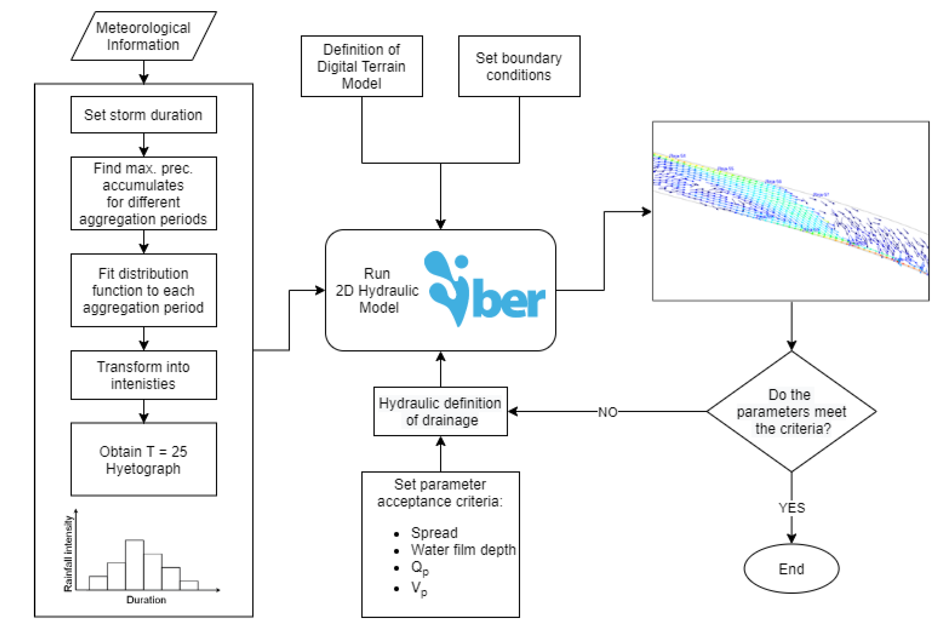
The methodology consisted of four steps: (1) obtaining the design hyetograph, (2) defining the road geometry as a digital terrain model, (3) setting parameter acceptance criteria, and (4) defining the hydraulic design of the drainage system by its implementation in the Iber model and analyzing simulation results. A workflow diagram of the methodology can be observed in Figure 1.
2.1. Design Hyetograph
The storm hyetograph is critical in drainage design since it determines the peak flooding volume in a catchment and the corresponding drainage capacity demand for a given return period [20]. Many approaches for defining design hyetographs can be found in the literature, such as the papers by Alfier et al. [21] and Balbastre-Soldevilla et al. [22].
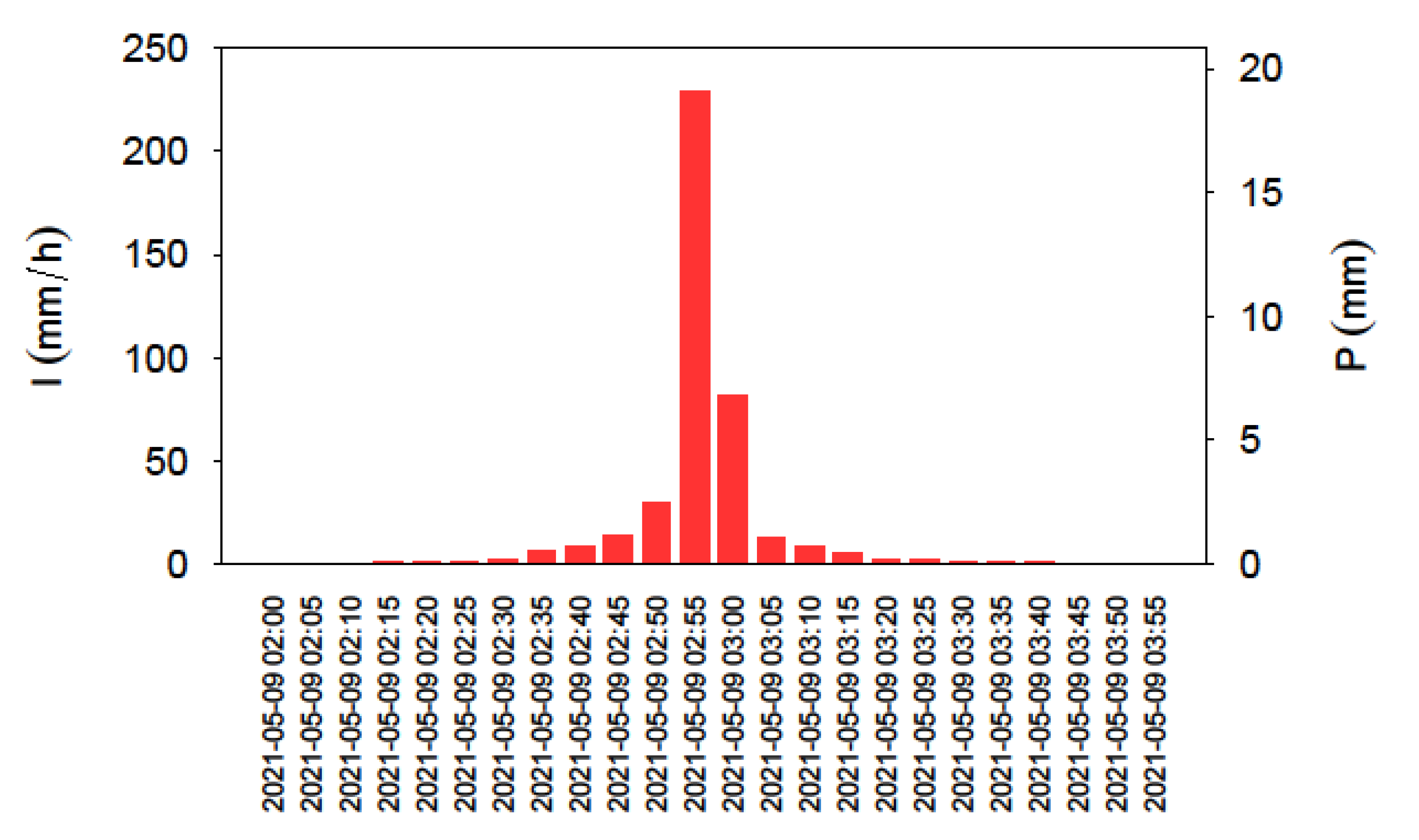
In the present study, the design hyetograph was built from existing observations at a 5-min temporal resolution. First, considering the time of concentration and the rainfall statistics of the study area, the duration of the design storm was set to two hours. Second, maximum precipitation accumulates for different aggregation periods up to the storm duration were calculated from the observations. The values for each aggregation period were fitted to different distribution functions, and the best fit was obtained with the square root normal distribution (SQRT). Last, the T = 25-year quantiles for each aggregation period were calculated and converted into intensities to build the 25-year return period hyetograph. For the construction of the design hyetograph following the method of Balbastre-Soldevila et al. [22], the Alternating Blocks Hyetograph Method [23] was selected.
2.2. Digital Terrain Model
A two-dimensional hydraulic model for the simulation of free surface flow requires three-dimensional information of the study area. This can be achieved by providing an elevation in the previously defined mesh. The higher the accuracy of the representation of topography, the better the model will perform. Different altimetric sources of information at different resolutions can be found in the literature. Mainly, these sources are (1) vector models based on entities, essentially points and lines, defined by their coordinates [24]; (2) raster models, in which each figure corresponds to the average value of elementary units of non-zero surface area that tessellate the terrain with a regular (matrix) distribution, without overlapping and with total coverage of the area represented [25]; and (3) light detection and ranging (LiDAR) models, in which point clouds are digital lists of points with x, y, and z coordinates and one or more descriptive attributes, including a point identifier. For more details, see Rutzinger et al., [26] and Zhao [27].
Casas et al. [28] compared the effects of the topographic data source and resolution on hydraulic modeling, concluding that LiDAR models presented the best results. These models can be applied when dealing with existing infrastructure in which a vectorial model is not available. However, in cases of new linear infrastructure in which vectorial models are available, as in our case study, LiDAR models will perform better since point elevations are perfectly defined for the entire model.
2.3. Parameter Acceptance Criteria
As discussed in the introduction, there are no common standardized criteria for drainage infrastructure design. Different approaches to limit excess surface water on roads can be found depending upon the design drainage standards of the country. However, there is a broad agreement among almost all standards to limit the values of four parameters: the generated storm peak flow, the total volume of water generated by the storm, and the water film thickness on the road and its spread.
The design criteria stated in the present paper are:
- The generated storm peak and the total volume of water associated with the storm will be obtained for a 25-year period [4].
- The water spread and water film thickness are limited to 1.5 m and 0.4 mm, respectively. Both values are lower than those proposed in different works, as discussed in Section 1.
As the case study is located in Spain, the aforementioned criteria are consistent with the recommendations of the Spanish standards. Nevertheless, the results presented in Section 4 are suitable to be applied to a different combination of design criteria according to the regulations in different countries.
2.4. Iber Model
Iber is a freely distributed 2D numerical tool (www.iberaula.com, accessed on 12 June 2021) initially developed for modeling hydrodynamic and sediment transport [19,24,25,26,27,28] that solves the SWEs on irregular geometries using the finite volume method (FVM). The tool has been continuously enhanced since it was first presented in 2010, and now includes a series of modules for different fluvial and hydrological processes, such as rainfall–runoff transformation [29,30,31], water quality processes [32,33], large wood transport [34], physical habitat suitability assessment [35], the consideration of pressurized flow [36,37,38,39], and, more recently, non-Newtonian flows such as wood-laden flows [40] and snow avalanches [41,42].
When applying Iber for the simulation of urban surface drainage problems, the source terms of the continuity equation must include rain intensity, infiltration, and the flow sinks due to the presence of drainage inlets toward the sewer system network [43]; thus, the governing equations are:
with
where is the flow thickness, . and . are the two velocity components on the horizontal directions of the unit discharge,
is the gravitational acceleration, and are the two bottom slope components, and and . are the two friction slope components, generally calculated with the Manning formula. For hydrological modeling (i.e., rainfall–runoff transformation) . accounts for the effect of rainfall on overland flow [44], . accounts for the rate of distributed hydrological losses (infiltration, evapotranspiration, and interception) [29], and . accounts for the distributed losses of surface water due to its incorporation with the drainage system. Iber solves these 2D-SWEs using a conservative scheme based on the FVM on an unstructured mesh of triangles and/or quadrilaterals. For the convective fluxes, it uses an explicit first-order Godunov-type upwind scheme [45], in particular, the Roe scheme [46].
In the case of road drainage systems constituted by grate inlets, . accounts for the discharge through inlets. The hydraulic capacity of a storm drainage inlet is a function of the grate type, gutter flow, and geometric road geometry. For the numerical modeling of road inlets, the classic methodology uses the hydraulic equations of weirs and orifices [47]. More recent methodologies are based on the concept of inlet efficiency [12]. With this approach, the efficiency of an inlet is defined as the ratio of the intercepted discharge by the inlet to the total discharge approaching the inlet:
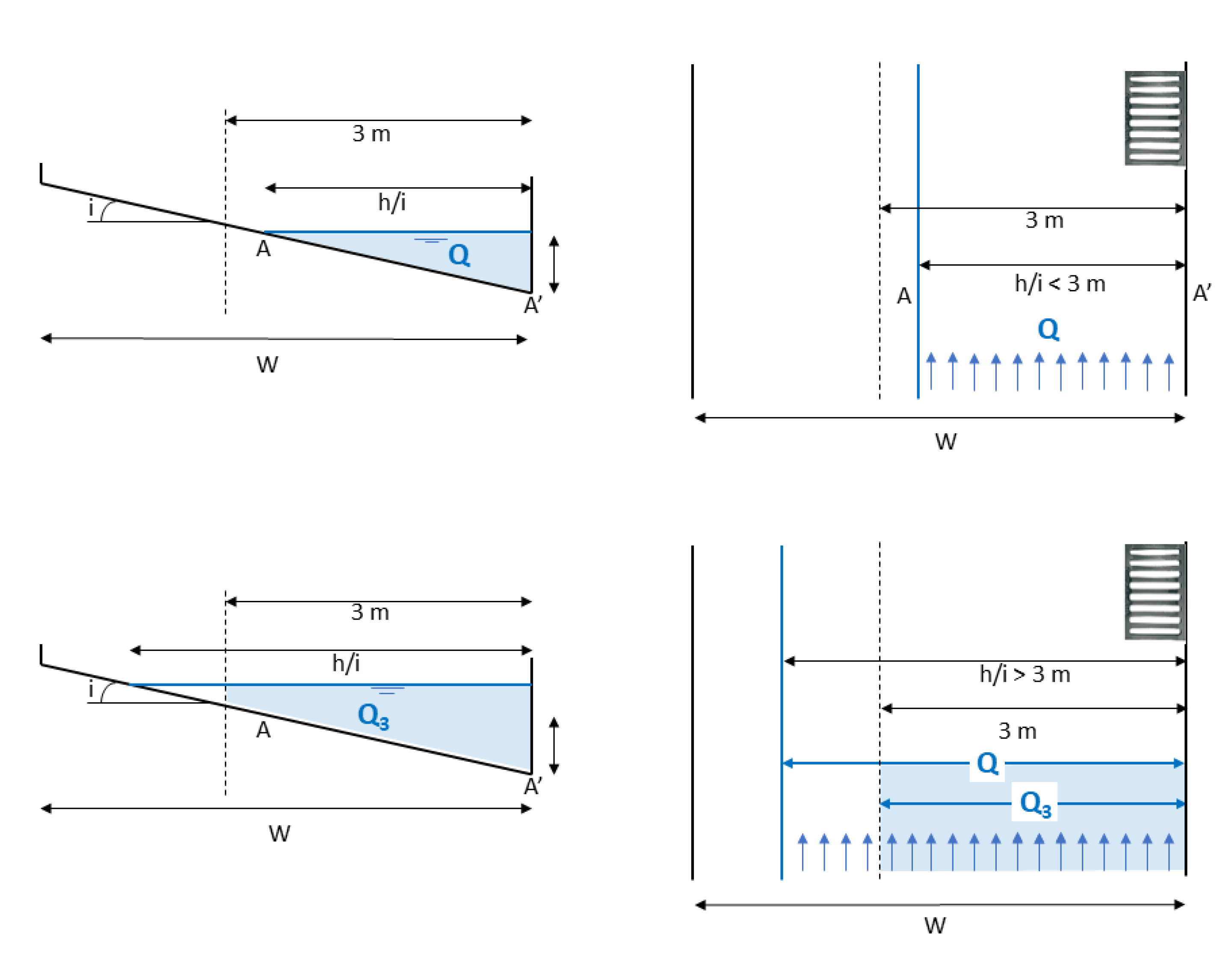
where E is the hydraulic inlet efficiency, Qint is the intercepted discharge by the inlet (m3/s), and Q3 is the total discharge approaching the inlet along a 3-m bandwidth of the roadway (Figure 2). The inlet efficiency can be estimated based on the knowledge of the grate characteristics (size, area, disposition, and number of holes) or the results of experimental laboratory tests [48]. This UPC methodology [48] proposes estimating the efficiency through a potential equation that relates the inlet efficiency with the flow thickness and the approximate rate flow through two characteristic parameters of the grate:
where A and B can be directly estimated with laboratory experience [9] or an approximate equation [49]. In the previous expressions, . is the discharge through a bandwidth of 3 m because the authors used an experimental facility representing a 3 m wide street [50]. For its inclusion in the formulation in the numerical model, the discharge . in this last equation is estimated as [43]:
where . is the transversal slope of the road at the inlet point.
With this approach, the efficiency of each inlet, which varies over time in an unsteady surface flow with the approaching flow, can be calculated from Equations (4) and (5) at each computational time step. Thus, together with Equation (3), the value of the discharge intercepted by the grate inlet ( can be obtained using the known road geometry, grate characteristics, and approaching over-road flow characteristics.
2.5. Location of Grate Inlets: Sensitivity Analysis
This section presents the strategy used to set the location of the grate inlets so that the criteria established in Section 2.3 are fulfilled. This strategy is based on a sensitivity analysis that assesses the configuration with the least number of grate inlets while satisfying the design criteria.
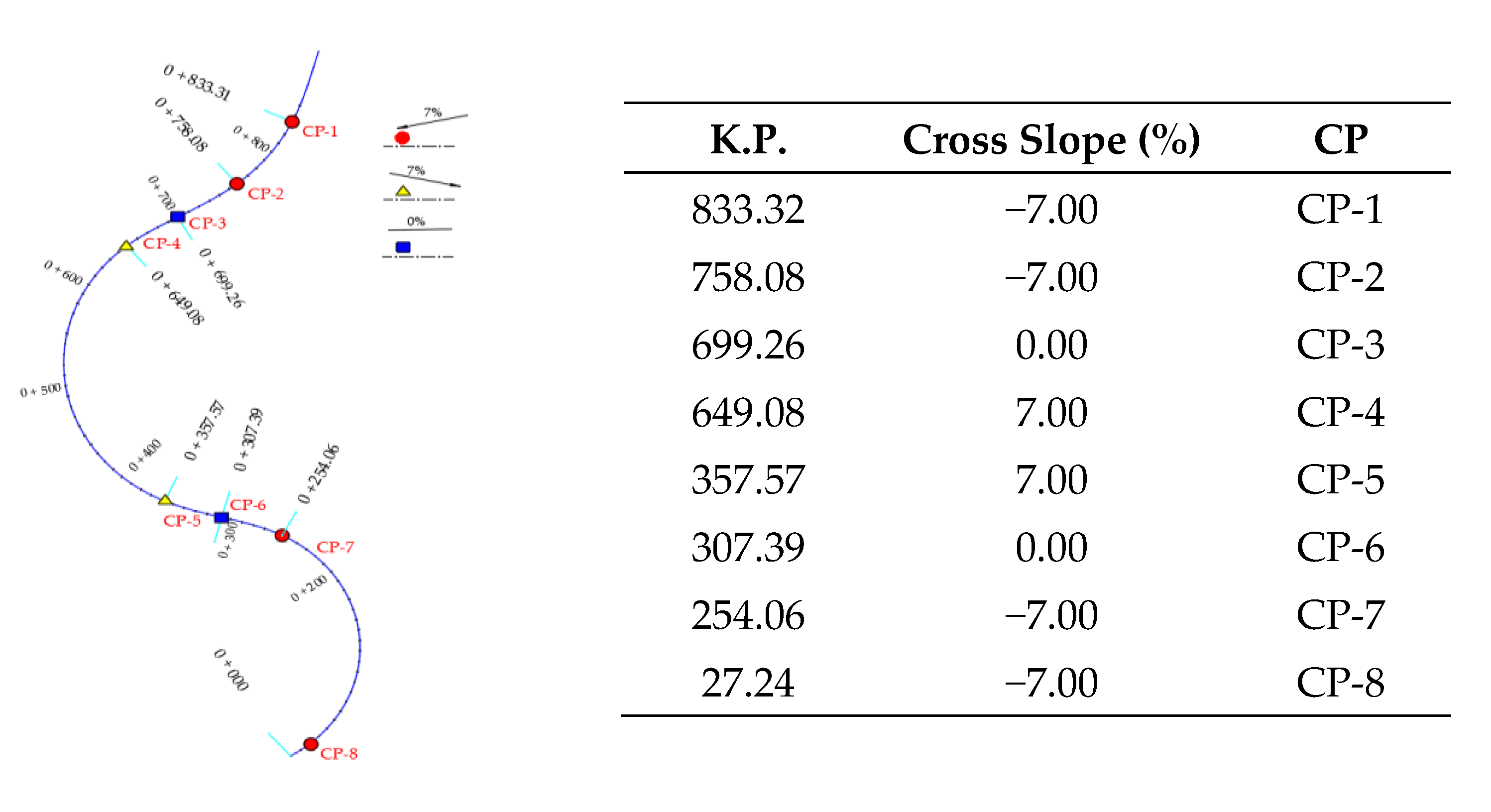
First, a set of critical points (hereafter referred to as control points) are identified. Their correct selection is critical for the implementation of the methodology since these are the locations where it will be verified that the criteria are met. Control points (CPs) must be located both at the beginning and at the end of any change in the road cross slope. The rationale behind this is that there is a change in the cross slope from these points onward, resulting in the formation of a flow across the road, which is precisely what it intends to prevent. Furthermore, additional control points may be placed in locations where the cross slope is zero as a consequence of the change of curvature. These control points are useful to characterize the potential flow across the road or the puddles formed by the stormwater.
Finally, grate inlets must be installed both at the beginning and the end of any change in the road cross slope. The rest of the grate inlets will be installed starting from these locations and in the upstream direction.
3. Case Study
3.1. Study Area
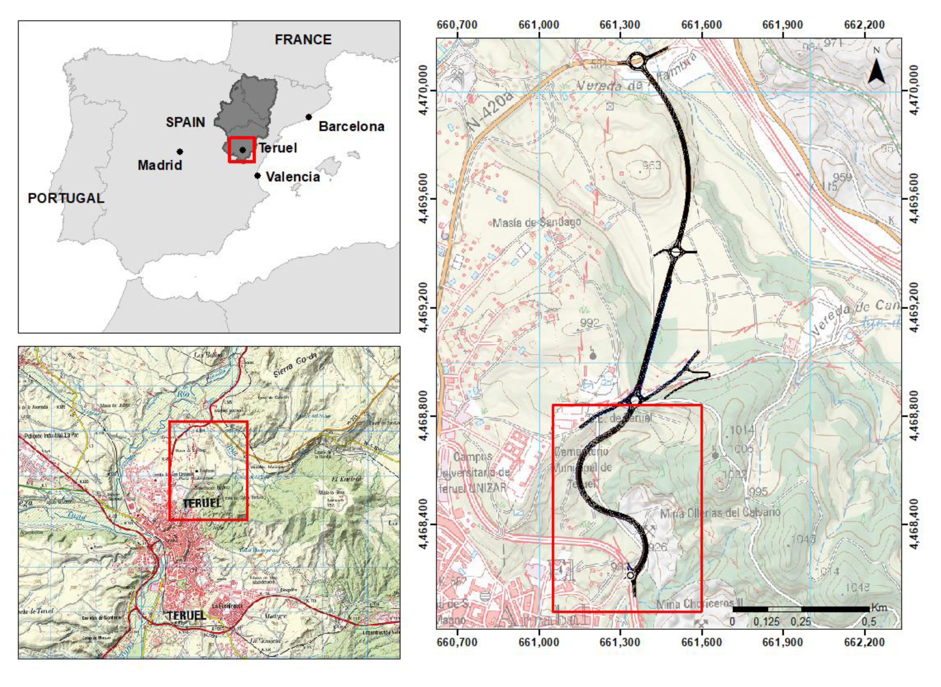
The proposed approach was implemented and evaluated in a section of road projected in the north of Teruel, Spain. This road will join the north of Teruel with the future city hospital, which is currently under construction. The project consists of a 2140-m two-lane dual carriageway, a footpath, and four new roundabouts: two located at either end of the road, linking with Conexión Barrios Ave to the south and N-420a to the north; one at chainage 0 + 819.69, which will provide access to the future hospital; and one at chainage 1 + 420, which will provide access to private properties (Figure 3).
For the purposes of the present study, only the stretch of road between the two southernmost roundabouts (i.e., chainage 0 + 000 to 0 − 818.69) was considered. Furthermore, in the case of the eastern carriageway, stormwater can flow freely and drain onto the embankment, whereas the designed footpath at a higher elevation than the roadway in the western carriageway acts as a barrier to stormwater, potentially leading to significant water thicknesses. For this reason, the eastern two-lane carriageway was also excluded from this study.
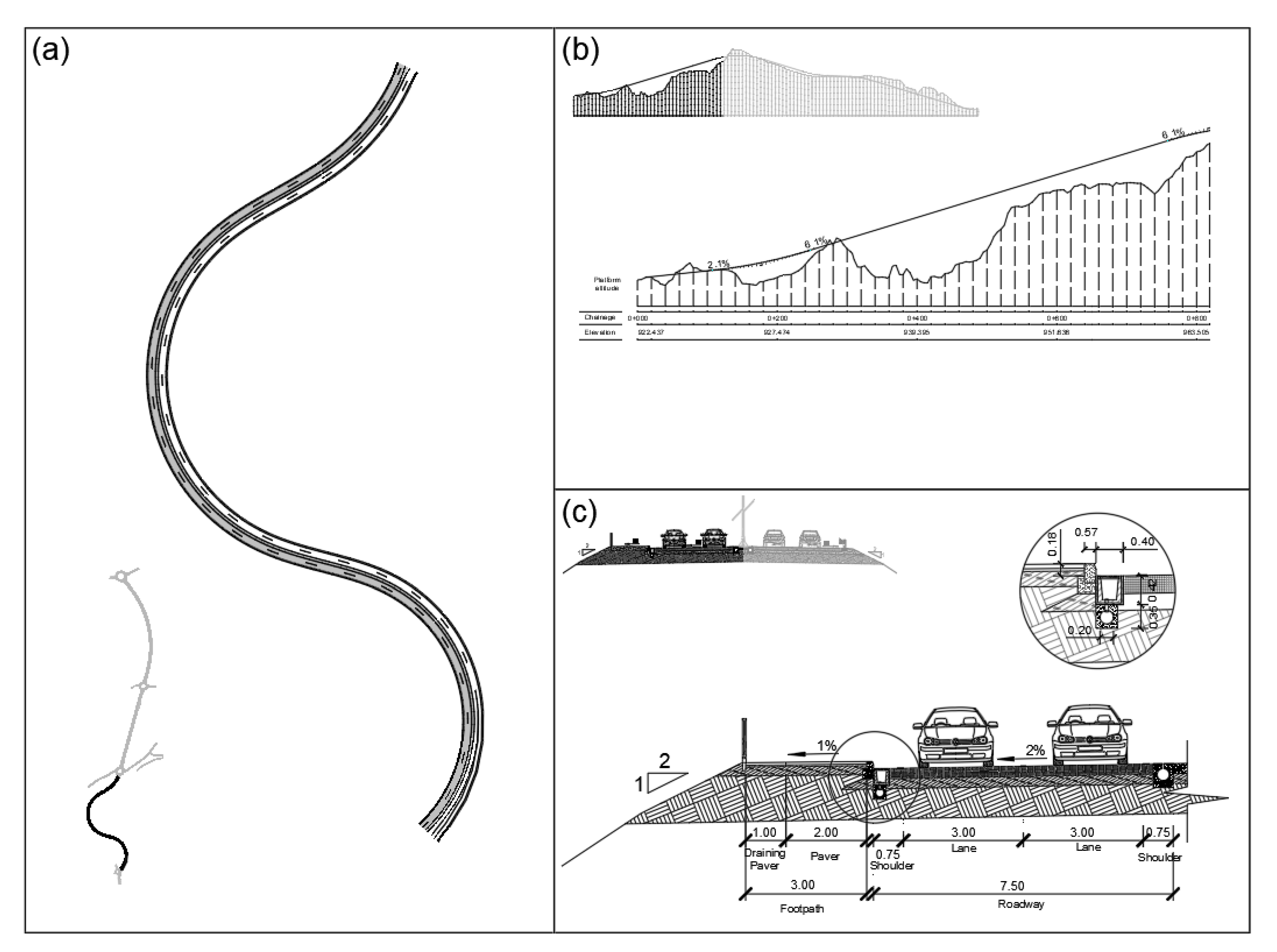
The horizontal alignment of the road consists of three consecutive curves (right, left, and right in the flow direction), with radiuses R = 170 m, R = 144 m, and R = 120 m, respectively (Figure 4a). Regarding the vertical alignment, the road is composed of two straight segments joined by a parameter Kv = 3500 m parabola. It starts at an elevation of 922.4 m.a.s.l. and finishes at 960.3 m.a.s.l., with design gradients of 2.1% on the first straight section of the road and 6.1% on the second (Figure 4b).
The cross-section (Figure 4c) consists of two 3-m-wide lanes plus a 0.75-m shoulder on each side with a design superelevation of 2%. The 3-m-wide footpath is detached from the roadway by a 0.18 m high curb, which prevents water from spilling over the footpath and facilitates drainage into the drainage channel and eventually into the gutters.
3.2. Data Collection and Climate Information
Meteorological information was obtained from the Júcar River Basin Authority (CHJ) through the Júcar Automatic Hydrological Information System (SAIH). Twenty-six full years of 5-min precipitation records (1995–2020) were available from the Arquillo reservoir rain gauge, which is located approximately 8 km west of the project area.
The observed average annual rainfall was 425 mm (Table 1). The annual precipitation pattern is highly controlled by the westerly winds associated with cold fronts, presenting the highest amounts of precipitation during spring and autumn. However, during the summer and at the beginning of the autumn, highly convective storms are typical in this area [51]. These rains are the focus of the present study due to their torrential intensity.
4. Results
4.1. Design Hyetograph
As mentioned in the methodology, the alternating blocks hyetograph method was used to obtain the design hyetograph. For a design storm of two hours and a return period of T = 25 years, the hyetograph below was obtained (Figure 5).
Considering a catchment area (i.e., road platform surface) of 6146 m2, the calculated design storm would discharge a total volume of water (Vt) of 796 m3, generating a peak flow of 373 L/s. These high values evidence the need to incorporate a series of drainage inlets that sink the stormwater toward the sewer system network.
4.2. Implementation in Iber Model
In this section, the results of the implementation of the Iber model are presented. First, the control point locations and grate inlet configurations were defined. Second, a sensitivity analysis for both the Manning roughness coefficient (n) and the mesh size (N) was conducted. Last, once these values were set, the model was run for each of the different grate inlet configurations.
4.2.1. Model Set-Up and Acceptance Criteria
In the study area, due to the three changes in the curvature of the stretch of road, six control points corresponding to the changes in the road cross slope were defined. Furthermore, two additional control points with cross slopes equal to zero (K.P. 307.39 and K.P. 699.26) were defined. The plan view (Figure 6) depicts the locations of the control points and the cross slope for each.
Once the control points were defined, different grate inlet configurations were designed. We proposed five main configurations in which the grate inlets are equidistantly installed every 10, 20, 30, 40, or 50 m from the control points. Table 2 summarizes the different configurations and the number of grate inlets to be installed.
Thresholds for the four parameters mentioned in the methodology were set, as shown in Table 3. Water film thickness and spread were set considering aquaplaning limitations, whereas the thresholds for Qp and Vp were fixed attending to the drainage capacity of the area, as described in Section 2.3.
4.2.2. Preliminary Analyses
Before comparing the results of the Iber model for the different inlet configurations, a sensitivity analysis for both n (Manning number) and N (mesh size), was carried out to assess how the variations of these parameters could affect the performance of the model.
Typical values for n in asphalt surfaces were 0.011 [52,53], 0.014 [54], and 0.016 [55]. Moreover, the Spanish standard 5.2 for road surface drainage recommends a value of n between 0.013 and 0.018 [4].
Thus, the sensitivity analysis was undertaken for values of n between 0.011 and 0.017 and for one of the proposed configurations (C1).
The results in the different control points are shown in Table 4. From these, a maximum variation of 0.7 cm can be observed, located in the areas where the cross slope is higher (7%).
It can also be observed that there is no significant difference for the control points where the cross slope is zero (K.P. 307.39 and K.P. 699.26; Figure 6). As opposed to the rest of the control points located in the road ditch, these two control points are located in the middle of the road, where high values of water film thickness could have potential implications for traffic (e.g., aquaplaning). Therefore, following the Spanish standard, a mean value for n of 0.015 was adopted.
Regarding the mesh size N, different model runs (configuration C1) were carried out for different cell sizes. A summary of the results can be observed in Table 5. Looking at the Vout and Qout (i.e., total volume and flow rate unable to be intercepted by the grate inlets) and the water film thickness at the control points, it can be concluded that from a mesh size of 1.23 by 0.48 m, results tend to stabilize. Therefore, this value was adopted for the rest of the simulations in this work.
4.2.3. Grate Inlet Configurations
Results obtained with the Iber model for the different grate inlet configurations are summarized next.
Table 6 shows the peak flow and the total volume generated by the design storm at the lowest point of the road (CP-8: K.P. 27.24) for the five configurations, considering no inlets (C0). A significant reduction of both peak flow and volume can be observed as the number of inlets installed increases.
Based on the spread (Table 7), it can be observed that configuration C1 (i.e., inlets equidistantly installed every 10 m) most closely meets the criteria set out in Section 2.3.
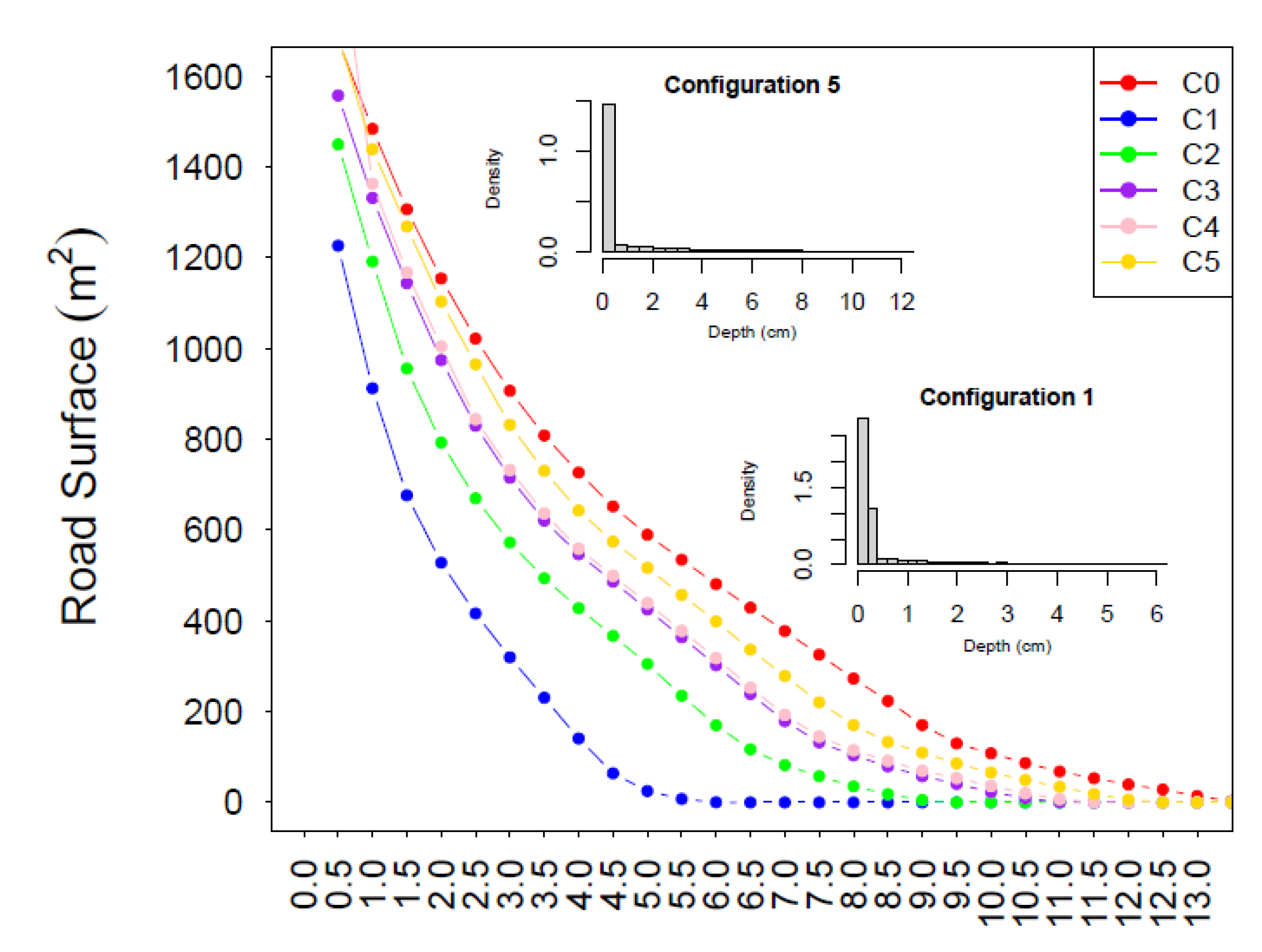
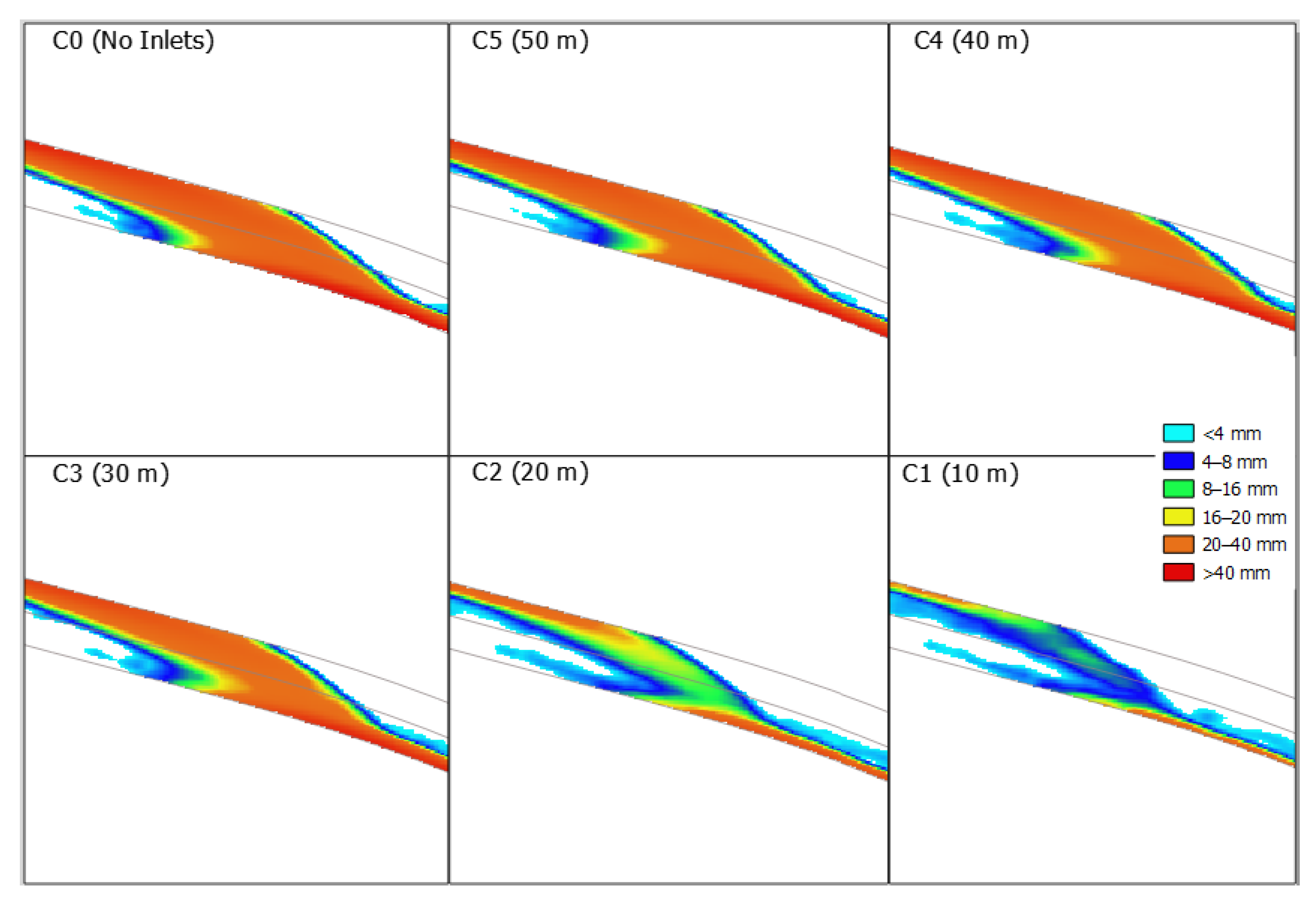
Regarding the water film thickness, Figure 7 shows a decrease of both water film thicknesses and flooded road surface when the number of grate inlets increases.
Furthermore, Table 8 shows the highest values reached for this parameter during the design storm. It is worth differentiating between the control points located in the road ditch and those located in the middle of the road. As expected, the former are associated with higher values since stormwater is confined by the curb. The latter (i.e., CPs 3 and 6), located where the cross slope is close to zero, present lower water film thicknesses but also indicate a flow across the road. Figure 8 shows the flow direction at CP 6 (K.P. 307.39).
Although this flow across the road reduces considerably in thickness with the number of grate inlets installed (Figure 8), even for configuration C1 it cannot be reduced enough to meet the criteria, which is a potential issue considering a critical threshold for aquaplaning of 0.4 cm [55].
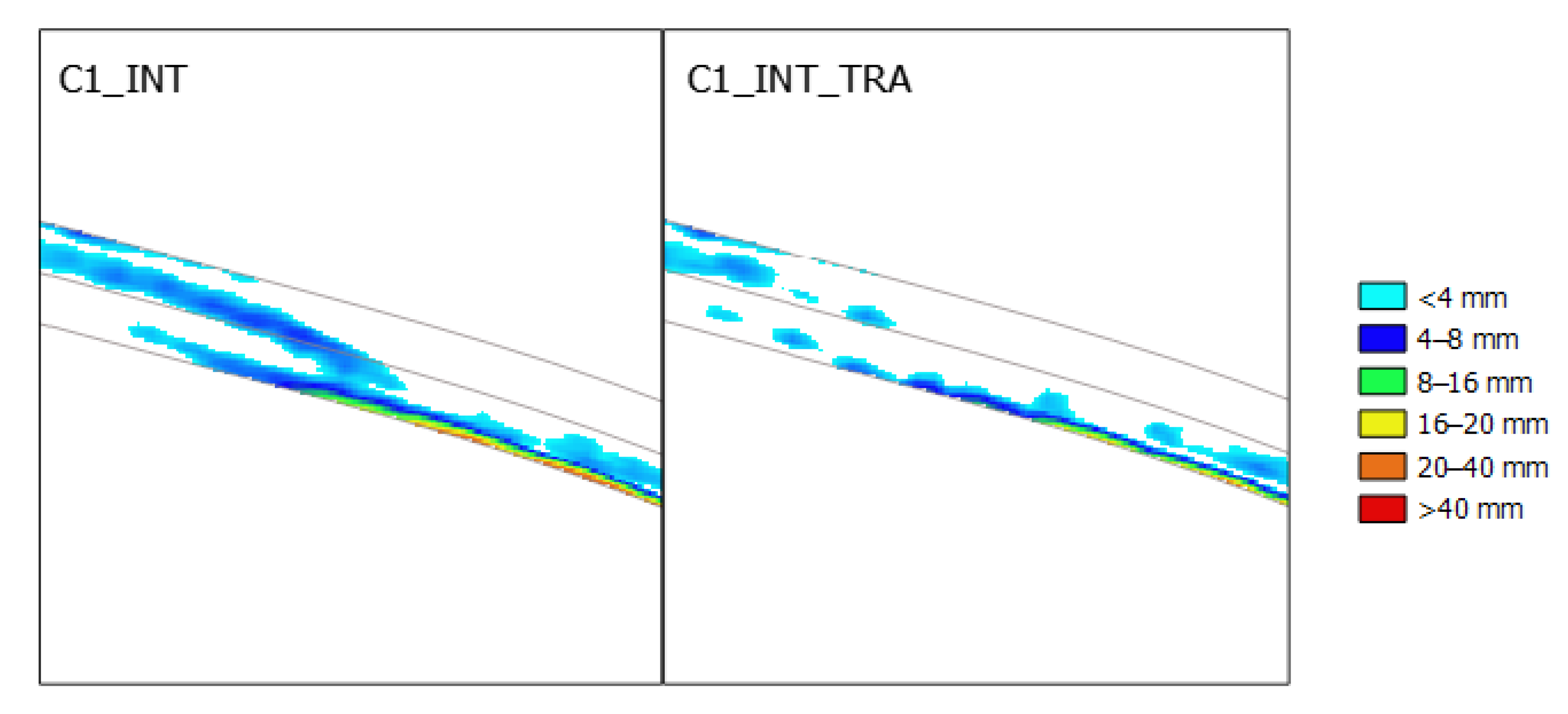
Based on these results showing that the water film criteria are not satisfied, and based on the flow direction on the road (Figure 8), two new configurations were implemented: (1) intensifying the number of grate inlets in locations close to the change in slope (C1_INT) and (2) intensifying the number of grate inlets in the same locations plus adding extra transverse grate inlets across the road (C1_INT_TRA).
These transverse grate inlets were placed at both the locations that presented flow across the road. For the purposes of the hydraulic Iber model, each transverse grate was formed by a set of 15 individual grate inlets placed side-by-side (which explains the large increase in the number of grate inlets).
The results of these two configurations are shown in Table 9. For better clarity, this table only shows the CPs located on the sections of the road where flow across the road was presented, which were therefore the areas most likely to present aquaplaning issues.
Table 9 and Figure 9 show that for configuration C1_INT_TRA (grate inlets installed at 10 m spacing, intensifying the number of grate inlets at points close to the locations where the cross slope is close to zero, and adding an extra grate inlet across the road), the water thickness criteria (<0.4 cm) is now met, reducing the flow across the road to small puddles.
5. Discussion
The proposed method for designing the location of grate inlets for the drainage of a road allows total control of the hydraulic behavior at each location. For each location, it is possible to perform a detailed analysis of its hydraulic behavior and obtain characteristic variables, such as the evacuated flow through it at each instant and its performance, estimated as the ratio between the flow rate approaching the grate inlet and the flow rate collected by it. Based on this comprehensive information, it is possible to make decisions about the relevance of a certain spacing between scuppers, the possibility of removing some of them without compromising the global drainage system performance, and the need to introduce a transverse grate inlet across the entire width of the road if adequate flow values are not obtained using only longitudinal ones.
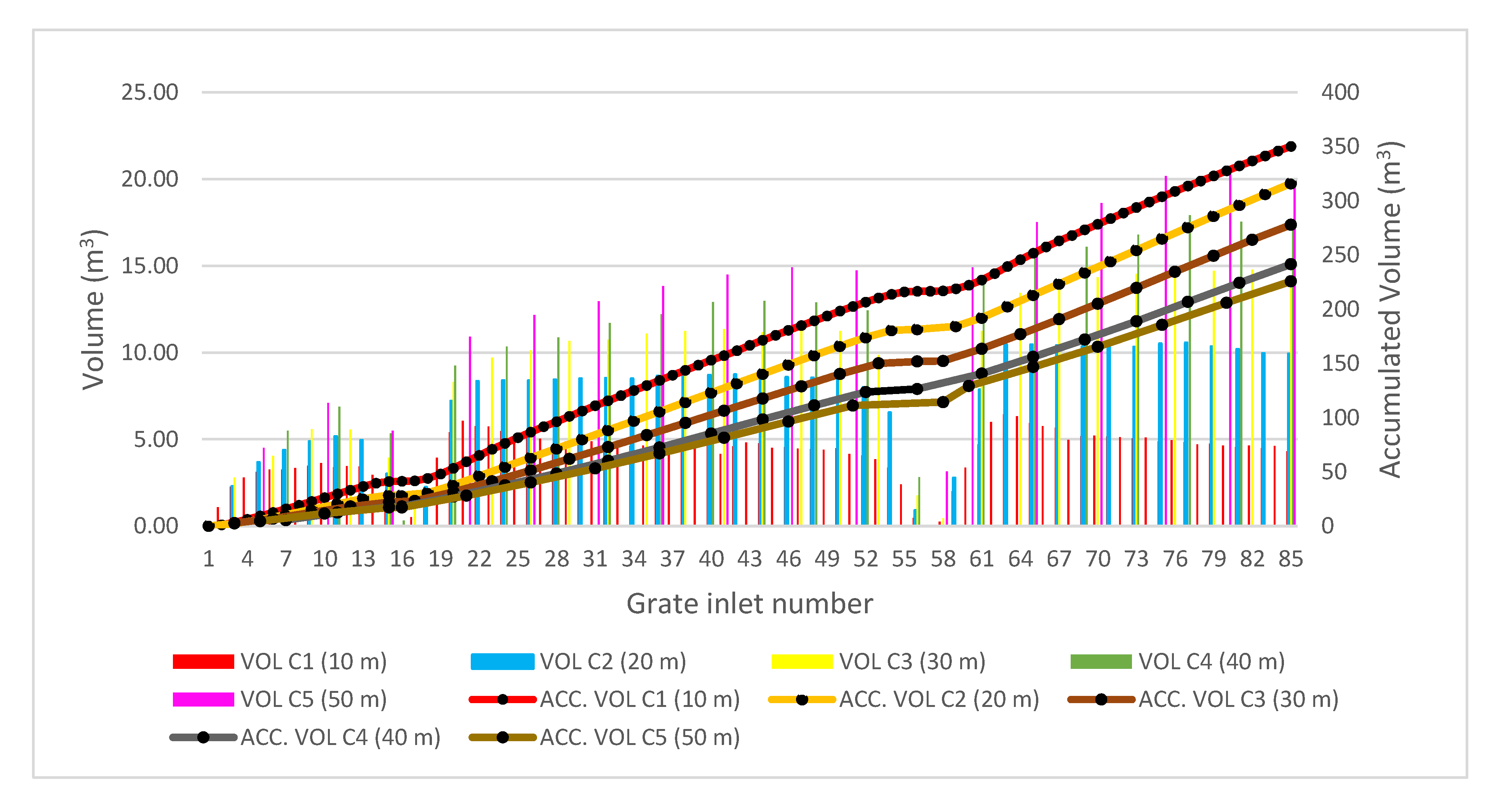
For the presented case study, Figure 10 shows the volume captured by each scupper and the accumulated captured volume along the road depending on the spacing between them. It can be clearly seen that with smaller spacing (and thus a higher number of grate inlets), the accumulated captured volume is greater, but the captured volume for each grate inlet is smaller.
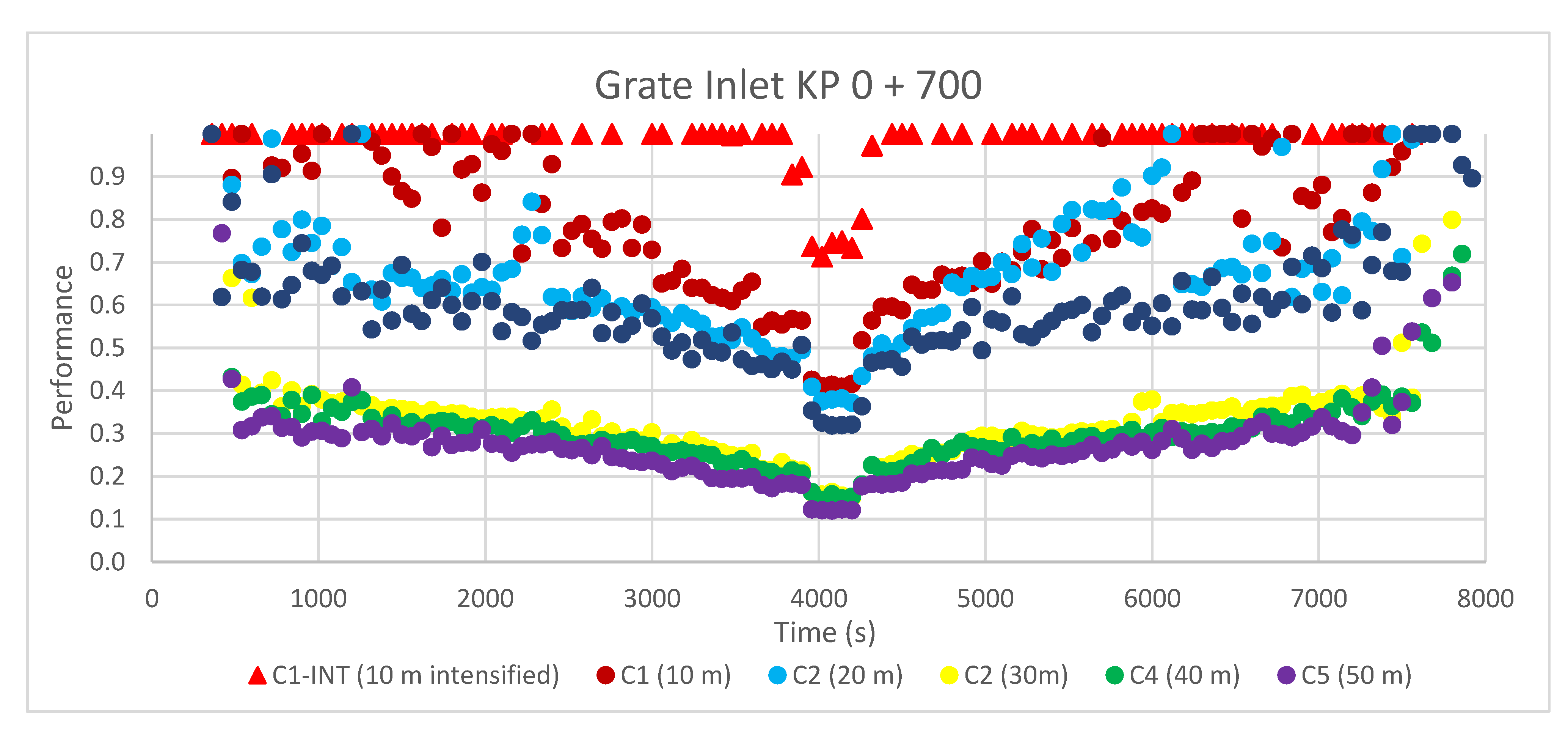
With the aim of analyzing the convenience of a particular inlet separation, the performance of grate inlets with distribution alternatives can be also analyzed by representing their hydraulic efficiency throughout the duration of the rainfall episode. This is shown in Figure 11 for the inlet located at KP 0 + 700 (Figure 6) and for different spacing distances between grates. A design with spacing C3 (30 m), C4 (40 m), and C5 (50 m) showed performances below 40%, with very small variations between configurations, which suggests that the upper efficiency limit for that particular road geometry was reached. By decreasing the distance between inlets, the efficiency of the inlet increases, which means that a greater portion of the discharge reaching them is captured. In this case, reasonably high values of efficiency were achieved with separations of C1 (10 m) and C2 (20 m), while in the case of C1_INT (10 m “intensified”), the efficiency was mostly equal to one. An efficiency of one for each inlet indicates that the entire flow approaching it is captured. This could be seen as a poor result in terms of the global efficiency of the drainage system; in other words, there are too many inlets, and a similar surface flow could be achieved with fewer inlets. In the presented inlet (KP 0 + 700), this would be the case for most of the rain episode, but not for the peak of the hyetograph, when the efficiency decreases to values of 0.7 and thus the proposed inlet distribution is justified.
Figure 12 shows a comparison of the performance for inlets located at KP 0 + 700 and KP 0 + 270 (see Figure 6) for a distance between inlets of C1_INT (10 m “intensified”). The inlet at KP 0 + 700 is located near the upstream end of the road. This means that the flow discharge reaching it is small and can be collected with high efficiency (1 for most of the simulation time). By contrast, the inlet at KP 0 + 270 receives a higher discharge and thus it is not able to capture all of it. Therefore, the efficiency graphs of Figure 11 and Figure 12 can be useful for fine-tuning the drainage design. A reasonable criterion would be a final drainage inlet distribution that achieves performances near or equal to one, but that with a slightly larger separation or rain intensity, the efficiency would drop to slightly lower than one, at least for the peak intensities. If the efficacy is still one with such an increase in separation or intensity, it means that the global design is not very efficient, as there are too many inlets.
In Figure 11 and Figure 12, the observed symmetry is due to the symmetry of the design rainfall scenario considered (Figure 5)
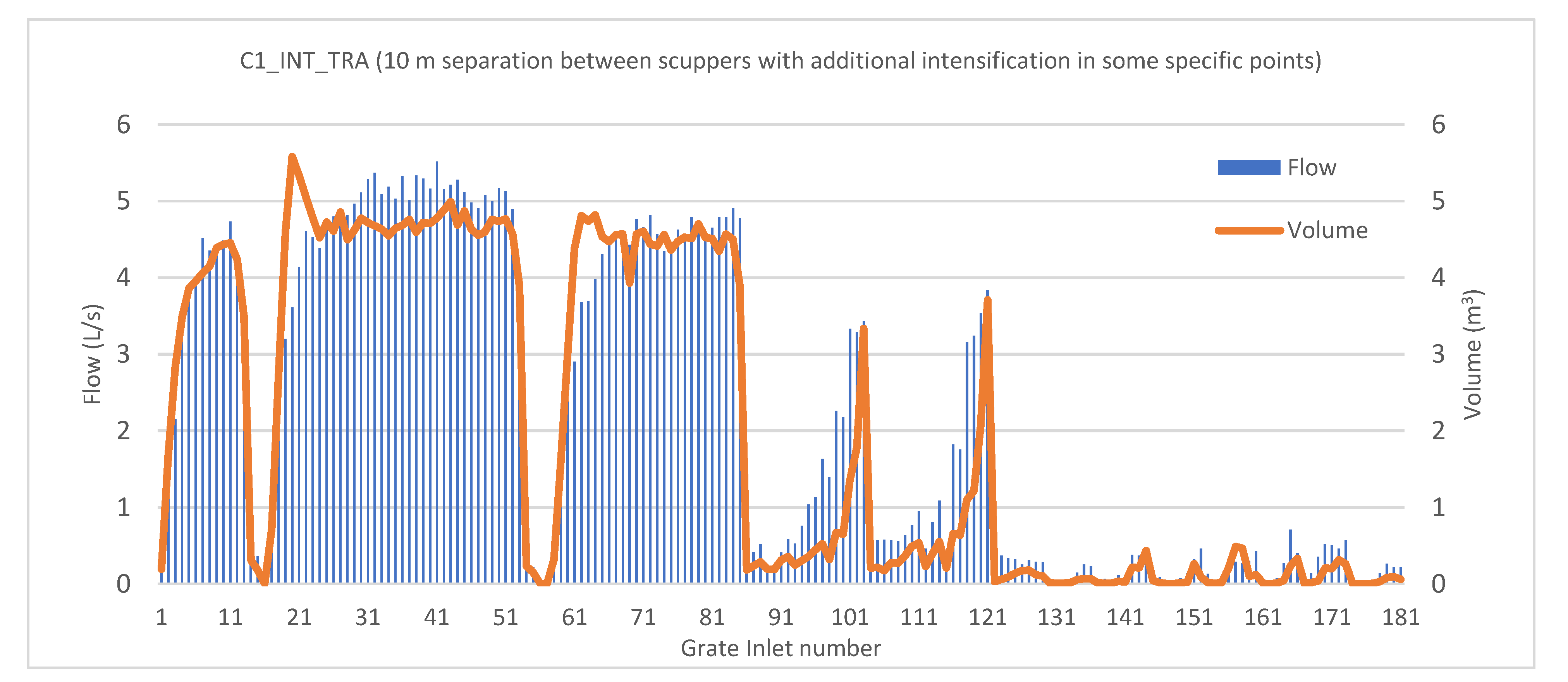
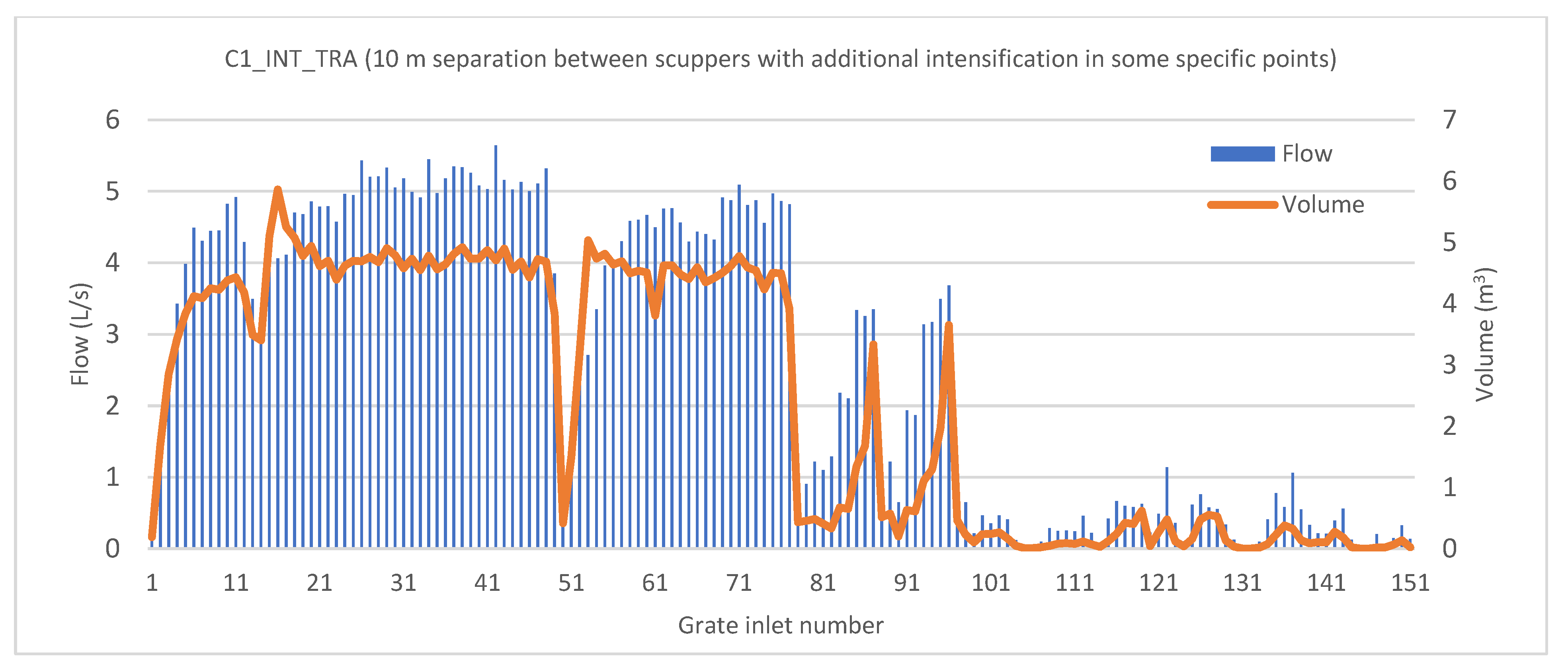
The analysis presented in Figure 10 opens the possibility for manually fine-tuning the inlet distribution or removing the most inefficient ones. In Figure 10, the flat regions of the accumulated volume curves at approximately inlet 16 and inlet 56 indicate that these inlets do not capture any flow, as there is little or no discharge approaching them. The same information can be presented for a particular case, for example, that of C1_INT_TRA, by representing the captured volume and discharge in every inlet, as shown in Figure 13. In this figure, the flat areas in Figure 10 are now represented as “valleys”. Additionally, a large number of inlets with little captured discharge can be observed at the right end of the graph. All these elements could be removed from the design. With such criteria, removing the inlets with a maximum captured discharge of less than 0.1 L/s results in the suppression of 30 inlets; thus, the total number is reduced from 181 to 151. The consequences on the captured discharge and volume of the remaining inlets are shown in Figure 14.
No substantial differences can be seen in Figure 14 compared with Figure 10, which indicates that the removed inlets were effectively unnecessary. In terms of final discharge and volume reaching the end of the road, the initial disposition C1_INT_TRA results in a maximum volume reaching this point of 362.5 m3, with a maximum discharge of 5.5 L/s. After the suppression of 30 unrequired inlets, the maximum value increases slightly to 363.1 m3/s, which represents a negligible increase of 0.17%; however, the maximum discharge increases to 5.6 L/s (1.8%), which justifies the removal of the selected inlets.
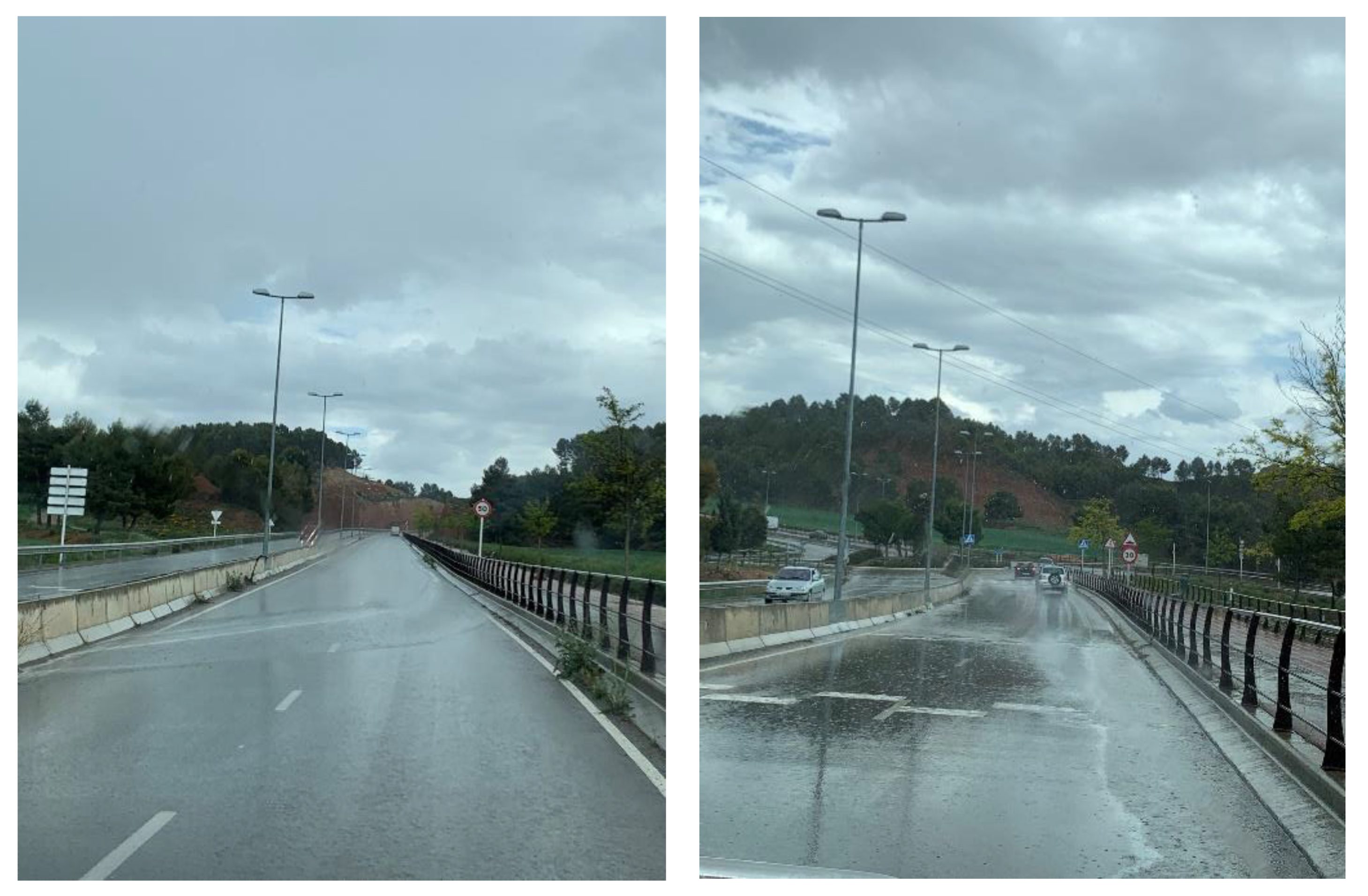
As already shown in Figure 8 and Figure 9, for a given inlet distribution and rainfall, the proposed method allows the prediction of hazardous scenarios likely to cause hydroplaning. The numerical results presented in Figure 8 and Figure 9 show a common situation in which the main water stream changes from one side of the road to the other as the road cant varies, similar to the images depicted in Figure 15.
6. Conclusions
A methodology for the design of road drainage systems by solving the 2D shallow water equations (using the Iber model [19]) in combination with the drainage inlet efficiency assessment equations of Gómez and Russo [8] was presented. The conclusions drawn from this methodology are as follows:
- −
- There are no common standard criteria for the design of drainage infrastructure, which depends on the design drainage standards of each country. However, there is a broad agreement within almost all standards to establish limits on the values of the generated storm peak flow, the total volume of water generated by the storm, and the water film thickness on the road and its spread.
- −
- The proposed method is suitable to be applied for a different combination of design criteria according to regulations in different countries.
- −
- The method, based on hydraulic numerical modeling using the Iber model, facilitates the analysis of different design scenarios, such as variations of the spacing between grate inlets. For any scenario, the results of the simulations make it possible to perform detailed analyses of their hydraulic behavior by providing characteristic variables, such as the evacuated flow through the drainage elements at each instant and their performance, estimated as the ratio between the flow rate approaching the grate inlet and the flow rate collected by it.
- −
- The method allows decision-making about the relevance of certain spacing distances between scuppers, the possibility of removing some of them without compromising the global drainage system performance, and the need to introduce a transverse grate inlet across the entire width of the road if adequate flow values are not obtained using only longitudinal ones.
Author Contributions
Conceptualization, J.Á.A., C.B., M.S.-J., and E.B.; methodology, J.Á.A. and C.B.; software, E.B.; validation, J.Á.A., C.B., M.S.-J., and E.B.; formal analysis, J.Á.A. and C.B.; investigation, J.Á.A., C.B., M.S.-J., and E.B.; resources, J.Á.A., C.B., M.S.-J., and E.B.; data curation, J.Á.A. and C.B.; writing—original draft preparation, C.B., M.S.-J., and E.B.; writing—review and editing, C.B., M.S.-J., and E.B.; visualization, J.Á.A.; supervision, J.Á.A., C.B., M.S.-J., and E.B.; project administration, J.Á.A., C.B., M.S.-J., and E.B. All authors have read and agreed to the published version of the manuscript.
Funding
This research received no external funding.
Institutional Review Board Statement
Not applicable.
Informed Consent Statement
Not applicable.
Data Availability Statement
Not applicable.
Acknowledgments
The authors wish to acknowledge support from Confederación Hidrográfica del Júcar, which provided the meteorological data used in the research.
Conflicts of Interest
The authors declare no conflict of interest.
References
- Hu, S.; Lin, H.; Xie, K.; Dai, J.; Qui, J. Impacts of Rain and Waterlogging on Traffic Speed and Volume on Urban Roads. In Proceedings of the IEEE Conference on Intelligent Transportation Systems, ITSC 2018, Maui, HI, USA, 4–7 November 2018; pp. 2943–2948. [Google Scholar] [CrossRef]
- Maze, T.H.; Agarwal, M.; Burchett, G. Whether weather matters to traffic demand, traffic safety, and traffic operations and flow. Transp. Res. Rec. 2006, 170–176. [Google Scholar] [CrossRef]
- Mukherjee, M.D. Highway Surface Drainage System & Problems of Water Logging In Road Section. Int. J. Eng. Sci. 2014, 3, 44–51. [Google Scholar]
- Ministerio de Obras Públicas y Urbanismo (M.O.P.U). Norma 5.2—IC—Drenaje Superficial de la Instrucción de Carreteras; Boletin Oficial del Estado (B.O.E.): Madrid, Spain, 2016. [Google Scholar]
- Brown, S.A.; Schall, J.D.; Morris, J.L.; Doherty, C.L.; Stein, S.M.; Warner, J.C. Urban Drainage Design Manual. Hydraul. Eng. Circ. 2013, 22, 478. [Google Scholar]
- Department of Energy and Water Supply. Queensland Urban Drainage Manual; Queensland Government: Brisbane, Australia, 2013. [Google Scholar]
- Li, X.; Fang, X.; Chen, G.; Gong, Y.; Wang, J.; Li, J. Evaluating curb inlet efficiency for urban drainage and road bioretention facilities. Water 2019, 11, 851. [Google Scholar] [CrossRef] [Green Version]
- Gómez, M.; Russo, B. Methodology to estimate hydraulic efficiency of drain inlets. In Institution of Civil Engineers: Water Management; Institution of Civil Engineers: London, UK, 2011; Volume 164, pp. 81–90. [Google Scholar] [CrossRef]
- Russo, B.; Gómez, M.; Tellez, J. Methodology to Estimate the Hydraulic Efficiency of Nontested Continuous Transverse Grates. J. Irrig. Drain. Eng. 2013, 139, 864–871. [Google Scholar] [CrossRef]
- Kim, J.S.; Kwak, C.J.; Jo, J.B. Enhanced method for estimation of flow intercepted by drainage grate inlets on roads. J. Environ. Manag. 2021, 279, 111546. [Google Scholar] [CrossRef] [PubMed]
- Wong, T.S.W. Kinematic wave method for determination of road drainage inlet spacing. Adv. Water Resour. 1994, 17, 329–336. [Google Scholar] [CrossRef]
- Nicklow, J.W.; Hellman, A.P. Optimal design of storm water inlets for highway drainage. J. Hydroinform. 2004, 6, 245–257. [Google Scholar] [CrossRef] [Green Version]
- Chesterton, J.; Nancekivell, N.; Tunnicliffe, N. The Use of the Gallaway Formula for Aquaplaning Evaluation in New Zealand. In Proceedings of the NZIHT Transit NZ 8th Annual Conference, Auckland, New Zealand, 15–17 October 2006; p. 22. [Google Scholar]
- Burlacu, A.; Răcănel, C.; Burlacu, A. Preventing aquaplaning phenomenon through technical solutions. Gradjevinar Croat. Assoc. Civ. Eng. 2018, 70, 1057–1064. [Google Scholar] [CrossRef] [Green Version]
- Department of Transport and Main Roads. Road Drainage Manual; Queensland Government: Brisbane, Australia, 2019. [Google Scholar]
- Amin, J.; Tohur, R. Surface Water Drainage of Roadway Using Concept of Permeable Pavement. Lambert Academic Publishing: Chisinau, Moldova, 2017. [Google Scholar]
- Lewis, M.; James, J.; Shaver, E.; Blackbourn, S.; Leahy, A.; Seyb, R.; Simcock, R.; Wihongi, P.; Sides, E.; Coste, C. Water Sensitive Design for Stormwater; Auckland Council: Auckland, New Zealand, 2015; ISBN 978-1-927216-43-9. [Google Scholar]
- Gibbons, J.L.; Bray, R.; O’Hare, T.; Coles, J.; Ayling, N.; Davies, O.; Hobbs, D.; Massini, P.; Monaghan, N.; Reid, K. SuDS in London: A Guide; Mayor of London: London, UK, 2016. [Google Scholar]
- Bladé, E.; Cea, L.; Corestein, G.; Escolano, E.; Puertas, J.; Vázquez-Cendón, E.; Dolz, J.; Coll, A. Iber: Herramienta de simulación numérica del flujo en ríos. Rev. Int. Metodos Numer. Calc. Diseno Ing. 2014, 30, 1–10. [Google Scholar] [CrossRef] [Green Version]
- Pan, C.; Wang, X.; Liu, L.; Huang, H.; Wang, D. Improvement to the huff curve for design storms and urban flooding simulations in Guangzhou, China. Water 2017, 9, 411. [Google Scholar] [CrossRef] [Green Version]
- Alfier, L.; Laio, F.; Claps, P. A simulation experiment for optimal design hyetograph selection. Hydrol. Process. 2008, 22, 813–820. [Google Scholar] [CrossRef]
- Balbastre-Soldevila, R.; García-Bartual, R.; Andrés-Doménech, I. A comparison of design storms for urban drainage system applications. Water 2019, 11, 757. [Google Scholar] [CrossRef] [Green Version]
- Te Chow, V.; Maidment, D.R.; Mays, L.W. Applied Hydrology; McGraw-Hill: New York, NY, USA, 1998; ISBN 0-07-100174-3. [Google Scholar]
- Bladé, E.; Cea, L.; Corestein, G. Numerical modelling of river inundations. Ing. Agua 2014, 18, 68. [Google Scholar] [CrossRef]
- Corestein, G.; Bladé, E.; Niñerola, D. Modelling bedload transport for mixed flows in presence of a non-erodible bed layer. In River Flow 2014; CRC Press: Lausanne, Switzerland, 2014; pp. 1611–1618. ISBN 9781138026742. [Google Scholar]
- Cea, L.; Bladé, E.; Corestein, G.; Fraga, I.; Espinal, M.; Puertas, J. Comparative analysis of several sediment transport formulations applied to dam-break flows over erodible beds. In Proceedings of the EGU General Assembly 2014, Vienna, Austria, 27 April–2 May 2014. [Google Scholar]
- Sanz-Ramos, M.; Olivares Cerpa, G.; Bladé i Castellet, E. Metodología para el análisis de rotura de presas con aterramiento mediante simulación con fondo móvil. Ribagua 2019, 6, 138–147. [Google Scholar] [CrossRef] [Green Version]
- Sanz-Ramos, M.; Bladé, E.; Escolano, E. Optimización del cálculo de la Vía de Intenso Desagüe con criterios hidráulicos. Ing. Agua 2020, 24, 203. [Google Scholar] [CrossRef]
- Cea, L.; Bladé, E. A simple and efficient unstructured finite volume scheme for solving the shallow water equations in overland flow applications. Water Resour. Res. 2015, 51, 5464–5486. [Google Scholar] [CrossRef] [Green Version]
- Fraga, I.; Cea, L.; Puertas, J. Effect of Rainfall Uncertainty on the Performance of Physically-Based Rainfall-Runoff Models Running Title Keywords Acknowledgments 1 Introduction. Hydrol. Process. 2019. [Google Scholar] [CrossRef] [Green Version]
- Sanz-Ramos, M.; Martí-Cardona, B.; Bladé, E.; Seco, I.; Amengual, A.; Roux, H.; Romero, R. NRCS-CN Estimation from Onsite and Remote Sensing Data for Management of a Reservoir in the Eastern Pyrenees. J. Hydrol. Eng. 2020, 25, 05020022. [Google Scholar] [CrossRef]
- Cea, L.; Bermúdez, M.; Puertas, J.; Bladé, E.; Corestein, G.; Escolano, E.; Conde, A.; Bockelmann-Evans, B.; Ahmadian, R. IberWQ: New simulation tool for 2D water quality modelling in rivers and shallow estuaries. J. Hydroinformatics 2016, 18, 816–830. [Google Scholar] [CrossRef] [Green Version]
- Anta Álvarez, J.; Bermúdez, M.; Cea, L.; Suárez, J.; Ures, P.; Puertas, J. Modelización de los impactos por DSU en el río Miño (Lugo). Ing. Agua 2015, 19, 105. [Google Scholar] [CrossRef]
- Ruiz-Villanueva, V.; Bladé, E.; Sánchez-Juny, M.; Marti-Cardona, B.; Díez-Herrero, A.; Bodoque, J.M. Two-dimensional numerical modeling of wood transport. J. Hydroinform. 2014, 16, 1077–1096. [Google Scholar] [CrossRef]
- Sanz-Ramos, M.; Bladé Castellet, E.; Palau Ibars, A.; Vericat Querol, D.; Ramos-Fuertes, A. IberHABITAT: Evaluación de la Idoneidad del Hábitat Físico y del Hábitat Potencial Útil para peces. Aplicación en el río Eume. Ribagua 2019, 1–10. [Google Scholar] [CrossRef] [Green Version]
- Cea, L.; López-Núñez, A. Extension of the two-component pressure approach for modeling mixed free-surface-pressurized flows with the two-dimensional shallow water equations. Int. J. Numer. Methods Fluids 2021, 93, 628–652. [Google Scholar] [CrossRef]
- Bladé, E.; Sanz-Ramos, M.; Dolz, J.; Expósito-Pérez, J.M.; Sánchez-Juny, M. Modelling flood propagation in the service galleries of a nuclear power plant. Nucl. Eng. Des. 2019, 352, 110180. [Google Scholar] [CrossRef]
- Aragón-Hernández, J.L.; Bladé, E. Modelación numérica de flujo mixto en conductos cerrados con esquemas en volúmenes finitos. Tecnol. Cienc. Agua 2017, 8, 127–142. [Google Scholar] [CrossRef] [Green Version]
- Bladé, E.; Gómez-Valentín, M.; Dolz, J.; Aragón-Hernández, J.L.; Corestein, G.; Sánchez-Juny, M. Integration of 1D and 2D finite volume schemes for computations of water flow in natural channels. Adv. Water Resour. 2012, 42, 17–29. [Google Scholar] [CrossRef]
- Ruiz-Villanueva, V.; Mazzorana, B.; Bladé, E.; Bürkli, L.; Iribarren-Anacona, P.; Mao, L.; Nakamura, F.; Ravazzolo, D.; Rickenmann, D.; Sanz-Ramos, M.; et al. Characterization of wood-laden flows in rivers. Earth Surf. Process. Landf. 2019, 44, 1694–1709. [Google Scholar] [CrossRef]
- Sanz-Ramos, M.; Bladé, E.; Torralba, A.; Oller, P. Las ecuaciones de Saint Venant para la modelización de avalanchas de nieve densa. Ing. Agua 2020, 24, 65–79. [Google Scholar] [CrossRef]
- Torralba, A.; Bladé, E.; Oller, P. Implementació d’un model bidimensional per a simulació d’allaus de neu densa. In Proceedings of the V Jornades Tècniques de Neu i Allaus: Pyrenean Symposium on Snow and Avalanches, Ordino, Andorra, 9–11 October 2017. [Google Scholar]
- Ramos-Fuertes, A.; Marti-Cardona, B.; Bladé, E.; Dolz, J. Envisat/ASAR Images for the Calibration of Wind Drag Action in the Doñana Wetlands 2D Hydrodynamic Model. Remote Sens. 2013, 6, 379–406. [Google Scholar] [CrossRef] [Green Version]
- Toro, E.F. Riemann Solvers and Numerical Methods for Fluid Dynamics; Springer: Berlin/Heidelberg, Germany, 2009; Volume 40, ISBN 978-3-540-25202-3. [Google Scholar]
- Roe, P.L. A basis for the upwind differencing of the two-dimensional unsteady Euler equations. In Numerical Methods for Fluid Dynamics II; Morton, K.W., Baines, M.J., Eds.; Springer: Berlin, Heidelberg, 1986; pp. 59–80. [Google Scholar]
- Guo, J.C.Y. Design of Street Curb Opening Inlets Using a Decay-Based Clogging Factor. J. Hydraul. Eng. 2006, 132, 1237–1241. [Google Scholar] [CrossRef] [Green Version]
- Engineers–Water Management; American Society of Civil Engineers: Reston, VA, USA, 2011; Volume 164, pp. 81–90. [CrossRef]
- Gómez, M.; Recasens, J.; Russo, B.; Martínez-Gomariz, E. Assessment of inlet efficiency through a 3D simulation: Numerical and experimental comparison. Water Sci. Technol. 2016, 74, 1926–1935. [Google Scholar] [CrossRef] [Green Version]
- Martínez-Gomariz, E.; Gómez, M.; Russo, B. Estabilidad de personas en flujos de agua. Ing. Agua 2016, 20, 43. [Google Scholar] [CrossRef] [Green Version]
- Moreno, A.; Sancho, C.; Bartolomé, M.; Oliva-Urcia, B.; Delgado-Huertas, A.; Estrela, M.J.; Corell, D.; López-Moreno, J.I.; Cacho, I. Climate controls on rainfall isotopes and their effects on cave drip water and speleothem growth: The case of Molinos cave (Teruel, NE Spain). Clim. Dyn. 2014, 43, 221–241. [Google Scholar] [CrossRef] [Green Version]
- Soil Conservation Service. In Urban Hydrology for Small Watersheds; Engineering Division, US Department of Agriculture: Huntington Park, CA, USA, 1986.
- McCuen, R. Hydrologic Analysis and Design Prentice Hall; Prentice-Hall: Englewood Cliffs, NJ, USA, 1989; Volume 850. [Google Scholar]
- Rodney, L.; Fangmeier, D.D.; Elliot, W.J.; Workman, S.R. Appendix B: Manning Roughness Coefficient. In Soil and Water Conservation Engineering, 7th ed.; American Society of Agricultural and Biological Engineers, St. Joseph, MI: Hoboken, NJ, USA, 2013; pp. 503–504. [Google Scholar]
- Chow, V.T. Open-channel hydraulics. In McGraw-Hill Civil Engineering Series; Kogakusha Ltd: Tokyo, Japan, 1959. [Google Scholar]
- Spitzhüttl, F.; Goizet, F.; Unger, T.; Biesse, F. The real impact of full hydroplaning on driving safety. Accid. Anal. Prev. 2020, 138. [Google Scholar] [CrossRef] [PubMed]
Figure 1.
Workflow diagram of the methodology.

Figure 2.
Calculation of , the equivalent discharge in a 3 m width, required for the efficiency estimation based on UPC methodology.
Figure 2.
Calculation of , the equivalent discharge in a 3 m width, required for the efficiency estimation based on UPC methodology.

Figure 3.
Study area: location map.

Figure 4.
Detail of infrastructure: (a) plan, (b) longitudinal profile, and (c) cross-section.

Figure 5.
Design hyetograph.

Figure 6.
Location of control points.

Figure 7.
Flooded road surface and maximum water film thickness for all configurations.

Figure 8.
Flow across CP-6 for all configurations.

Figure 9.
Flow across the road at K.P. 307 (C1_INT and C1_INT_TRA).

Figure 10.
Captured volume at each grate inlet (vertical lines) and accumulated volumes (longitudinal profiles) depending on the spacing between them.
Figure 10.
Captured volume at each grate inlet (vertical lines) and accumulated volumes (longitudinal profiles) depending on the spacing between them.

Figure 11.
Performance of inlet located at KP 0 + 700 (Figure 6) for different spacing distances between grates. The performance is represented as the ratio between the flow rate that enters the cell containing the grate and the flow rate collected by it.
Figure 11.
Performance of inlet located at KP 0 + 700 (Figure 6) for different spacing distances between grates. The performance is represented as the ratio between the flow rate that enters the cell containing the grate and the flow rate collected by it.

Figure 12.
Comparison of the performance for inlets located at KP 0 + 700 and KP 0 + 270 (Figure 6).
Figure 12.
Comparison of the performance for inlets located at KP 0 + 700 and KP 0 + 270 (Figure 6).

Figure 13.
Captured volume and discharge for each inlet in scenario C1_INT_TRA (10 m separation between scuppers with additional intensification at some specific points).
Figure 13.
Captured volume and discharge for each inlet in scenario C1_INT_TRA (10 m separation between scuppers with additional intensification at some specific points).

Figure 14.
Captured volume and discharge for each inlet in scenario C1_INT_TRA (10 m separation between scuppers with additional intensification at some specific points).
Figure 14.
Captured volume and discharge for each inlet in scenario C1_INT_TRA (10 m separation between scuppers with additional intensification at some specific points).

Figure 15.
Flow across the road likely to cause hydroplaning (author: Beatriz Aranda).


Table 1.
Precipitation records/statistics of Arquillo reservoir rain gauge: Left, highest intensities registered for different aggregation periods; Right, mean monthly precipitation.
Table 1.
Precipitation records/statistics of Arquillo reservoir rain gauge: Left, highest intensities registered for different aggregation periods; Right, mean monthly precipitation.
| Aggregation Period (min) | Precipitation (mm) | I (mm/h) | Date |  |
| 5’ | 23.52 | 282.24 | 13/09/1999 | |
| 10’ | 24.72 | 148.32 | 25/08/2017 | |
| 15’ | 31.20 | 124.80 | 19/06/2009 | |
| 30’ | 43.68 | 87.36 | 13/07/2006 | |
| 60’ | 76.32 | 76.32 | 13/07/2006 |
Table 2.
Grate inlet configurations.
| Configuration | Nº of grate inlets |
|---|---|
| No grate inlets (C0) | 0 |
| 10 m spacing (C1) | 85 |
| 20 m spacing (C2) | 43 |
| 30 m spacing (C3) | 29 |
| 40 m spacing (C4) | 21 |
| 50 m spacing (C5) | 18 |
Table 3.
Acceptance criteria.
| Parameter | Threshold | Units |
|---|---|---|
| Water film thickness | <0.4 | mm |
| Spread | <1.5 | m |
| Qp | <10 | L/s |
| Vt | <20 | m3 |
Table 4.
Sensitivity analysis for n in the different control points for configuration C1. Values indicate water film thickness in cm.
Table 4.
Sensitivity analysis for n in the different control points for configuration C1. Values indicate water film thickness in cm.
| CP | n = 0.017 | n = 0.015 | n = 0.013 | n = 0.011 |
|---|---|---|---|---|
| CP-1 | 2.5 | 2.3 | 2.2 | 2.1 |
| CP-2 | 2.7 | 2.7 | 2.6 | 2.3 |
| CP-3 | 0.6 | 0.6 | 0.6 | 0.6 |
| CP-4 | 2.5 | 2.4 | 2.2 | 1.8 |
| CP-5 | 1.9 | 2.0 | 1.8 | 1.5 |
| CP-6 | 0.6 | 0.5 | 0.4 | 0.4 |
| CP-7 | 1.9 | 1.8 | 1.6 | 1.5 |
| CP-8 | 1.1 | 0.8 | 0.7 | 0.6 |
Table 5.
Sensitivity analysis for mesh size in the different control points for configuration C0. Vout and Qout indicate the total volume and flow rate unable to be intercepted by the grate inlets, respectively.
Table 5.
Sensitivity analysis for mesh size in the different control points for configuration C0. Vout and Qout indicate the total volume and flow rate unable to be intercepted by the grate inlets, respectively.
| Nº of divisions | N = 1 | N = 2 | N = 4 | N = 6 | N = 8 | ||||||
|---|---|---|---|---|---|---|---|---|---|---|---|
| lx − ly | x | y | x | y | x | y | x | y | x | y | |
| Size (m) | 4.90 | 1.91 | 2.45 | 0.96 | 1.23 | 0.48 | 0.82 | 0.32 | 0.61 | 0.24 | |
| Vout (m3) | 375.00 | 374.82 | 372.36 | 372.24 | 372.66 | ||||||
| Qout (L/s) | 343 | 344 | 343 | 342 | 343 | ||||||
| Thickness (cm) | CP-1 | 0.8 | 1.3 | 1.8 | 2.3 | 2.4 | |||||
| CP-2 | 2.6 | 3.5 | 4.3 | 5.0 | 5.4 | ||||||
| CP-3 | 2.3 | 1.7 | 1.5 | 1.4 | 1.4 | ||||||
| CP-4 | 4.2 | 5.7 | 6.9 | 7.1 | 7.6 | ||||||
| CP-5 | 7.3 | 8.9 | 10.0 | 10.5 | 11.2 | ||||||
| CP-6 | 4.0 | 3.6 | 3.6 | 3.6 | 3.6 | ||||||
| CP-7 | 7.4 | 9.8 | 11.2 | 11.5 | 11.7 | ||||||
| CP-8 | 10.8 | 13.8 | 15.6 | 16.4 | 16.9 | ||||||
Table 6.
Peak flow and total volume at CP-8 (K.P. 27.24) for the different grate inlet configurations.
Table 6.
Peak flow and total volume at CP-8 (K.P. 27.24) for the different grate inlet configurations.
| Configuration | N° of Inlets | Q (L/s) | V (m3) |
|---|---|---|---|
| No grate inlets (C0) | 0 | 372.7 | 386.0 |
| 10 m spacing (C1) | 85 | 9.9 | 18.0 |
| 20 m spacing (C2) | 43 | 21.1 | 37.0 |
| 30 m spacing (C3) | 29 | 98.8 | 180.0 |
| 40 m spacing (C4) | 21 | 131.5 | 222.0 |
| 50 m spacing (C5) | 18 | 156.1 | 243.0 |
Table 7.
Spread for the different grate inlet configurations in the different CPs.
| CP | Spread (cm) | |||||
|---|---|---|---|---|---|---|
| C0 | C5 | C4 | C3 | C2 | C1 | |
| CP-1 | 285 | 225 | 220 | 210 | 180 | 95 |
| CP-2 | 430 | 430 | 400 | 335 | 180 | 95 |
| CP-3 | 750 | 690 | 690 | 670 | 475 | 375 |
| CP-4 | 368 | 350 | 325 | 160 | 155 | 95 |
| CP-5 | 450 | 450 | 410 | 135 | 110 | 95 |
| CP-6 | 750 | 690 | 690 | 640 | 411 | 400 |
| CP-7 | 380 | 380 | 380 | 120 | 95 | 85 |
| CP-8 | 90 | 75 | 75 | 75 | 75 | 60 |
Table 8.
Water film thickness (cm) in the eight control points for the different configurations.
| CP | Flow Thickness (cm) | |||||
|---|---|---|---|---|---|---|
| C0 | C5 | C4 | C3 | C2 | C1 | |
| CP-1 | 1.4 | 1.4 | 1.4 | 1.4 | 1.3 | 0.9 |
| CP-2 | 4.0 | 3.7 | 3.8 | 3.4 | 2.2 | 1.7 |
| CP-3 | 1.2 | 1.1 | 1.1 | 1.0 | 0.7 | 0.5 |
| CP-4 | 6.1 | 5.2 | 5.7 | 5.5 | 4.2 | 2.5 |
| CP-5 | 8.7 | 7.9 | 7.5 | 6.6 | 3.6 | 2.3 |
| CP-6 | 2.9 | 2.3 | 2.3 | 2.1 | 0.9 | 0.8 |
| CP-7 | 10.0 | 8.7 | 8.4 | 8.0 | 4.9 | 3.3 |
| CP-8 | 14.5 | 10.8 | 10.4 | 9.6 | 4.0 | 2.4 |
Table 9.
Water film thickness (cm) in CP-3 and CP-6 for the two new configurations.
| CP | C1_INT | C1_INT_TRA |
|---|---|---|
| CP-3 | 0.5 | 0.4 |
| CP-6 | 0.6 | 0.4 |
Publisher’s Note: MDPI stays neutral with regard to jurisdictional claims in published maps and institutional affiliations. |
© 2021 by the authors. Licensee MDPI, Basel, Switzerland. This article is an open access article distributed under the terms and conditions of the Creative Commons Attribution (CC BY) license (https://creativecommons.org/licenses/by/4.0/).
Share and Cite
MDPI and ACS Style
Aranda, J.Á.; Beneyto, C.; Sánchez-Juny, M.; Bladé, E. Efficient Design of Road Drainage Systems. Water 2021, 13, 1661. https://doi.org/10.3390/w13121661
AMA Style
Aranda JÁ, Beneyto C, Sánchez-Juny M, Bladé E. Efficient Design of Road Drainage Systems. Water. 2021; 13(12):1661. https://doi.org/10.3390/w13121661
Chicago/Turabian StyleAranda, José Ángel, Carles Beneyto, Martí Sánchez-Juny, and Ernest Bladé. 2021. "Efficient Design of Road Drainage Systems" Water 13, no. 12: 1661. https://doi.org/10.3390/w13121661
Note that from the first issue of 2016, this journal uses article numbers instead of page numbers. See further details here.