New Insights into the Seasonal Variation of DOM Quality of a Humic-Rich Drinking-Water Reservoir—Coupling 2D-Fluorescence and FTICR MS Measurements

Abstract

Long-term changes in dissolved organic matter (DOM) quality, especially in humic-rich raw waters, may lead to intensive adaptions in drinking-water processing. However, seasonal DOM quality changes in standing waters are poorly understood. To fill this gap, the DOM quality of a German drinking water reservoir was investigated on a monthly basis by Fourier-transform ion cyclotron resonance mass spectrometry (FTICR MS) measurements and 2D fluorescence for 18 months. FTICR MS results showed seasonal changes of molecular formula (MF) intensities, indicating photochemical transformation of DOM as a significant process for DOM quality variation. For an assessment of the two humic-like components, identified by parallel factor analysis (PARAFAC) of excitation–emission matrices (EEM), their loadings were Spearman’s rank-correlated with the intensities of the FTICR MS-derived MF. One of the two PARAFAC components correlated to oxygen-rich and relatively unsaturated MF identified as easily photo-degradable, also known as coagulants in flocculation processes. The other PARAFAC component showed opposite seasonal fluctuations and correlated with more saturated MF identified as photo-products with some of them being potential precursors of disinfection byproducts. Our study indicated the importance of elucidating both the chemical background and seasonal behavior of DOM if raw water-quality control is implemented by bulk optical parameters.

1. Introduction

For several decades, drinking-water reservoirs in the Northern Hemisphere have been affected by a long-lasting increase in dissolved organic carbon (DOC) from catchment areas [1,2,3]. Investigations into raw waters have shown that photochemical and microbial transformations can have an influence on the DOM quality in drinking-water reservoirs [4,5,6] and other stratified lakes [7]. Until now only minor information has been available regarding how and whether DOM quality undergoes seasonal changes in drinking-water reservoirs. However, this appears to be an important subject for research, as a part of the DOC is usually removed from raw waters [8,9,10]. Several studies have documented this part of the DOC, which is mainly subjected to coagulation, and some studies have noted the chemical composition of this dissolved organic matter part, the molecules of which potentially act as precursors for halogenated disinfection byproducts [4,11,12,13,14,15]. Nevertheless, changes in DOM quality in raw waters can lead to substantial consequences for the drinking-water treatment procedure. These results thus provide essential information regarding the estimation of the level of technical expense with respect to drinking-water processing. Furthermore, they provide fresh scientific knowledge relating to seasonal DOM quality variations in a drinking-water reservoir, and to the quality as a function of water depth.

Numerous studies over a long period of time have shown that, in order to characterize the DOM in waters, the DOC determination as the bulk parameter has been a common and standardized method [16], as along with UV_{254 nm} and the Specific UV Absorbance (SUVA) [4,11]. As the bulk parameter, it offers general information regarding the quantity of DOM, but only limited information regarding the composition of the DOM [17]. UV_254nm, in combination with DOC and other basic water chemistry parameters has already been used to successfully predict disinfection byproduct formation potential from raw water quality (by modelling using artificial neural networks) [18,19,20]. Some studies, e.g., [21,22], have shown that the fDOM had a good correlation with the DOC because fDOM captures a sufficient amount of the DOC pool, although DOC compounds do exist that cannot be measured with the fDOM sensor [21]. This is one of the reasons why we used a fluorescence spectrometer with a resolution much higher than one wavelength, and combined the EEMs with the parallel factor analysis (PARAFAC). Since the year 2000, more and more investigators have used 2D-fluorescence excitation–emission matrices (EEM) to provide more information regarding the DOM group composition, to at least distinguish between the protein/tryptophan-like and humic-like chromophores [23,24]. Based on these results, PARAFAC as a chemometric tool has become increasingly important with respect to extracting the main information from the 2D-fluorescence excitation–emission matrices [25,26]. In this way, it was possible to identify the fluorescence peaks as a cluster of different chromophoric subgroups such as free amino acids or proteins, low-molecular-weight humic acids common in wetlands and agricultural environments, high-molecular-weight humic acids, and aromatic humics, with high abundance in wetlands and forested environments [27].

The calculation of PARAFAC components from the individual fluorescence spectra have been used to describe the seasonal dynamics of the fDOM [28]. The focus of this particular study was to investigate the influence of the wet and dry seasons. Two protein-like and two humic-like components were found with significant seasonal variations. The CDOM was linked to DOC and salinity. No resolution of DOM quality as function of lake depth was available. Wang et al. [29] investigated spatial variations of DOM quality, in addition to the seasonal variations. Different locations at lake surface level, albeit not as a function of depth, were sampled for resolution of horizontal/longitudinal variations. Bracchini et al. investigated the variation of DOM quality as a function of lake depthalong with additional seasonal variations [7]. They showed epilimnetic photo-bleaching of CDOM in summer and an increase in algae-derived CDOM. Through differentiation of ultrafiltration they showed that CDOM absorption corresponded to low-molecular-weight compounds in the epilimnion and higher-molecular-weight compounds in the hypolimnion.

Up until now, research has been carried out on seasonal and spatial resolution of DOM quality. However, the above-mentioned studies used bulk and/or bulk optical parameters with relatively low chemical resolution. In one of our recent studies (Herzsprung et al., 2020) [30], data from high-resolution Fourier-transform ion cyclotron resonance mass spectrometry (FTICR MS) in a drinking-water reservoir (Rappbode Reservoir) is available as a function of time and depth, providing the most recent, highest resolution with respect to DOM chemical composition. The research gap, however, is the combination of bulk optical parameters—which can be determined to be cost–effectively and with relatively low laboratory effort using large amounts of samples—with the sophisticated high-resolution FTICR MS on selected samples, in particular for seasonal and spatial variations of DOM quality in the water body of a lake or reservoir. The combination of fluorescence measurements with FTICR MS via rank correlation used is based on a study [31] where results from high-field FTICR MS and bulk optical parameters were combined to show differences in DOM of rewetted and natural peatlands. Stubbins et al. (2014) [32] linked PARAFAC results based on EEMs with the outcome of FTICR MS measurements.

In the knowledge that seasonal and vertical DOM quality differences exist in drinking-water reservoirs, we hypothesized that: (i) more low-molecular-weight components would be present and detectable by FTICR MS measurements in summer because of the photochemical transformations; (ii) combining FTICR MS results with EEMs by intersample rank correlations, it is possible to show that photochemical processes destroy higher-molecular-weight fluorophore substances and form smaller fluorophore molecules; and (iii) the combination of the concomitant parameter with the PARAFAC model offers the possibility to interpret the PARAFAC components in more detail.

To test the hypotheses, monitoring of the Muldenberg drinking-water reservoir in the Ore Mountains, Saxony, Germany, was carried out in order to detect seasonal DOM quality variations over a time period of 18 months in 2015–2016. Beyond the interpretation of the 2D-fluorescence EEMs linked to the results of analyzed samples with FTICR MS [33], the determination of the “routine” parameters of DOC, as well as UV_254nm and SUVA, were used to combine them with the PARAFAC model.

2. Materials and Methods

2.1. Study Area and Sampling

This study was conducted at the Muldenberg drinking water reservoir (main dam) located in Saxony, Germany (lat: 50.401847, lon: 12.380528) at an altitude of 770 m above sea level. The reservoir is relatively small (0.81 km²) and shallow, with a maximum depth of 14 m depth. The reservoir has two light-flooded pre-dams, which are fed by shady tributaries. In the catchment area of the study zone, there is no agriculture or settlements given that this region is a drinking-water protection zone according to the German Water Resources Law, § 51 and § 52 [34]. Water samples were collected monthly from three different depths (0 m (surface water); 9−13 m (depth of the raw water extraction) and 14 m (bottom water)) of the drinking-water reservoir, between February 2015 and July 2016, resulting in 16 sampling times. The pH, water temperature (°C), conductivity (µS cm⁻¹), and dissolved oxygen concentration (DO) (mgL⁻¹) were measured on site. For the purpose of further analysis, all collected samples were stored at 4 °C during transport as well as in the laboratory before sample preparation and analysis.

2.2. Characterization of Fluorescent Dissolved Organic Material

For the determination of the fluorescent DOM (fDOM), filtered water samples were measured using Aqualog^® (Horiba Jobin Yvon, Edison, NJ, USA) at an excitation range of 240 to 600 nm with 1 nm increments, and an emission range of 212 to 621 nm with 0.42 nm (1 pixel) increments, using a quartz cuvette of 1 cm path length. The integration time was 1 s. All measured excitation–emission matrices (EEMs) were blank-subtracted (Milli-Q^TM water) and, corrected for instrument-specific biases and inner filter effects for each measurement (time point). Additionally, the EEMs were normalized to the Raman and Rayleigh (first and second radiation) area (10 nm) of Milli-Q water.

In order to acquire information from three-dimensional data matrices, the fDOM components were identified by parallel factor analysis (PARAFAC) using SOLO (Eigenvector Research, Inc., Manson, DC, USA). For a detailed description of the multiway decomposition method for PARAFAC, see [35,36].

Using PARAFAC modeling, each sample set was decomposed, dependent on a predefined number of components (N) using Equation (1) [37,38]:

$$x_{ijk}={\displaystyle \sum }_{f=1}^N{a}_{if}{b}_{jk}{c}_{kf}+e_{ijk}$$

(1)

The value of ith sample is $x_{ijk}$, the emission wavelength is jth, and the excitation wavelength is kth. Here, $e_{ijk}$ is the respective residuum; i.e., data not modeled by PARAFAC components. The variables a (samples), b (emission), and c (excitation) are matrices (also called modes) with N columns and multiple rows, equal to the numbers of samples, emission wavelengths, or excitation wavelengths, respectively.

The current PARAFAC model was developed using 48 EEMs from 3 depths in the main dam each sampled 16 times, and was validated using split-half validation, core consistency diagnostics, and visual inspection of the residuals [39] (as shown in Table S1, fluorescence data is available for 48 out of 54 samples). The halves of the split-half validation agreed at 98.2% for Mode 2 (emission loadings) as well as for Mode 3 (excitation loading) (Figure S9).

2.3. Solid-Phase Extraction (SPE) and FTICR MS Measurements

For the FTICR MS measurements, aliquots of 50 mL of the acidified filtrate (pH 2 with HCl) were passed through solid-phase extraction cartridges (Bond Elut PPL, 500 mg, Agilent, Waldbronn, Germany) to desalt the extract for subsequent electrospray ionization (ESI) mass spectrometry (MS) using an automatic cartridge extractor (Horizon Technology, Salem, NH, USA). The SPE-DOM was eluted with 2 × 2 mL methanol, diluted with methanol to 5 mL, and kept frozen until analysis [40,41].

An FTICR mass spectrometer equipped with a dynamically harmonized analyzer cell (solariX XR, Bruker Daltonics Inc., Billerica, MA, USA) and a 12 T refrigerated, actively-shielded superconducting magnet (Bruker Biospin, Wissembourg, France) instrument, was used in negative ESI mode (capillary voltage: 4.5 kV) at the ProVIS Centre for Chemical Microscopy which is part of the Helmholtz Centre for Environmental Research. Extracts were analyzed in random order with an autosampler (infusion rate: 10 µL min⁻¹). Mass spectra were recorded with a 4 MW time domain as 256 transients were co-added in the mass range of m/z 150–100, and molecular formulas were subsequently assigned to mass peaks in the range of m/z 150–750 with an error range of ±0.5 ppm [42]. Molecular formulas were calculated considering the following elements: ¹²C_1–60, ¹³C_0–1, ¹H_1–122, ¹⁶O_0–40, ¹⁴N_0–2, ³²S_0–1, and ³⁴S_0–1. Only formulas with double-bound equivalents (DBEs) 0 ≤ DBEs ≤ 25 and −10 ≤ DBEs-O ≤ 10 were considered for further data evaluation [43,44]. Molecular formulas (MFs) present in full process blanks were removed from the entire data set if their peak intensity was, on at least one occasion, higher than the lowest intensity within the 54 samples. Relative peak intensities (RIs) were calculated based on the summed intensities of all assigned peaks in each sample [45]. A total of 2232 MFs were found to be present in all 54 samples, as specified in Table S2 (data base provided in Excel). The optical and basic water chemistry parameters are listed in Table S1.

2.4. Correlation between fDOM, PARAFAC Components, and FTICR MS Components

The significance of intensity change with time was first calculated using a robust Spearman’s rank correlation [3]. The Spearman’s rank correlation coefficient is a quantitative measure for assessing the strength of the relationship between two continuous or quantitatively discrete features. The calculation is similar to the Pearson correlation, whereby the ranks of the measured values are used and not the measured values themselves. A value of +1 indicates a strictly monotonically increasing relationship between the values of two features. A value of −1 indicates a strictly monotonically decreasing relationship. If there is no monotonous relationship, the Spearman’s rank correlation coefficient assumes values close to zero. The classical Pearson correlation or product–moment correlation could not be used since the relationship of the two variables used was not linear and did not follow a bivariate normal distribution [46].

The p-values were calculated from the r_s values as a function of the sample number n, and were adjusted for multiple testing using the Benjamini–Hochberg correction (FDR-adj. p-values; 5% false discovery rate) [47,48].

As prearrangement for rank correlation of the fluorescence indices and PARAFAC component loadings with the MF intensities (of those MFs which were present in all 48 samples), the intensity ranks for all 107,136 (2232 × 48) MFs at all depths and time points samples were calculated. For DOC and SUVA, 122,760 (2232 × 54) MFs were used. The intensity ranks were used for calculation of the intersample ranks (ranking of each component in all samples) [3,6,31]. The intersample ranks were used for calculation of rank correlation coefficients with the concomitant parameters (DOC, SUVA, and fluorescence indices).

2.5. Concomitant Parameters

2.5.1. Concentration and Absorbance of Dissolved Organic Carbon (DOC)

The DOC concentration was determined according to DIN EN 1484:2019–04 standard [16] using a DIMATOC 2000 (Dimatec Analysentechnik GmbH, North Rhine Westphalia, Germany), including preacidification to remove the DIC. UV absorbance was measured using a DR 5000 spectro-photometer (Hach Lange GmbH, North Rhine Westphalia, Germany) at a wavelength of 254 nm, using a quartz cuvette with a 1 cm path length [16].

2.5.2. Calculation of the Specific Ultraviolet Absorbance

The specific UV absorbance (SUVA) was calculated using the log10 light absorption coefficient at 254 nm (m⁻¹) normalized to DOC (mgC L⁻¹). The SUVA is highly correlated to a hydrophobic organic fraction of DOM [49]. Higher values are associated with greater aromatic content [50]. SUVA values >4 indicate mainly hydrophobic and especially aromatic material, while values <3 indicate mainly hydrophilic material [51].

2.5.3. Calculation of the Fluorescence Indices: HIX, BIX, and FI

The humification index (HIX) was calculated as a ratio of areas under the emission curve at 435 nm and 480 nm, such as 300 and 345 nm plus 435 and 480 nm, at an excitation wavelength of 254 nm [52]. HIX values between 0 and 1 indicated the degree of fDOM humification (high HIX = more humic material). The fluorescence index (FI) was calculated as the ratio between the emission signals at 470 nm and 520 nm obtained at 370 nm excitation [53]. FI values of ≈1.8 indicated microbial origin, and FI values of ≈1.3 indicated terrestrial origin. The biological index (BIX) was calculated as the ratio of the emission intensity at 380 nm divided by the emission intensity maximum observed between 420 and 435 nm, obtained at excitation of 310 nm [54]. BIX values indicated the age of the DOM, with higher values demonstrating a larger contribution of more freshly produced DOM [55]. All fluorescence indices were calculated using Python 3.7.1 (Python Software Foundation, Beaverton, OR, USA).

3. Results and Discussion

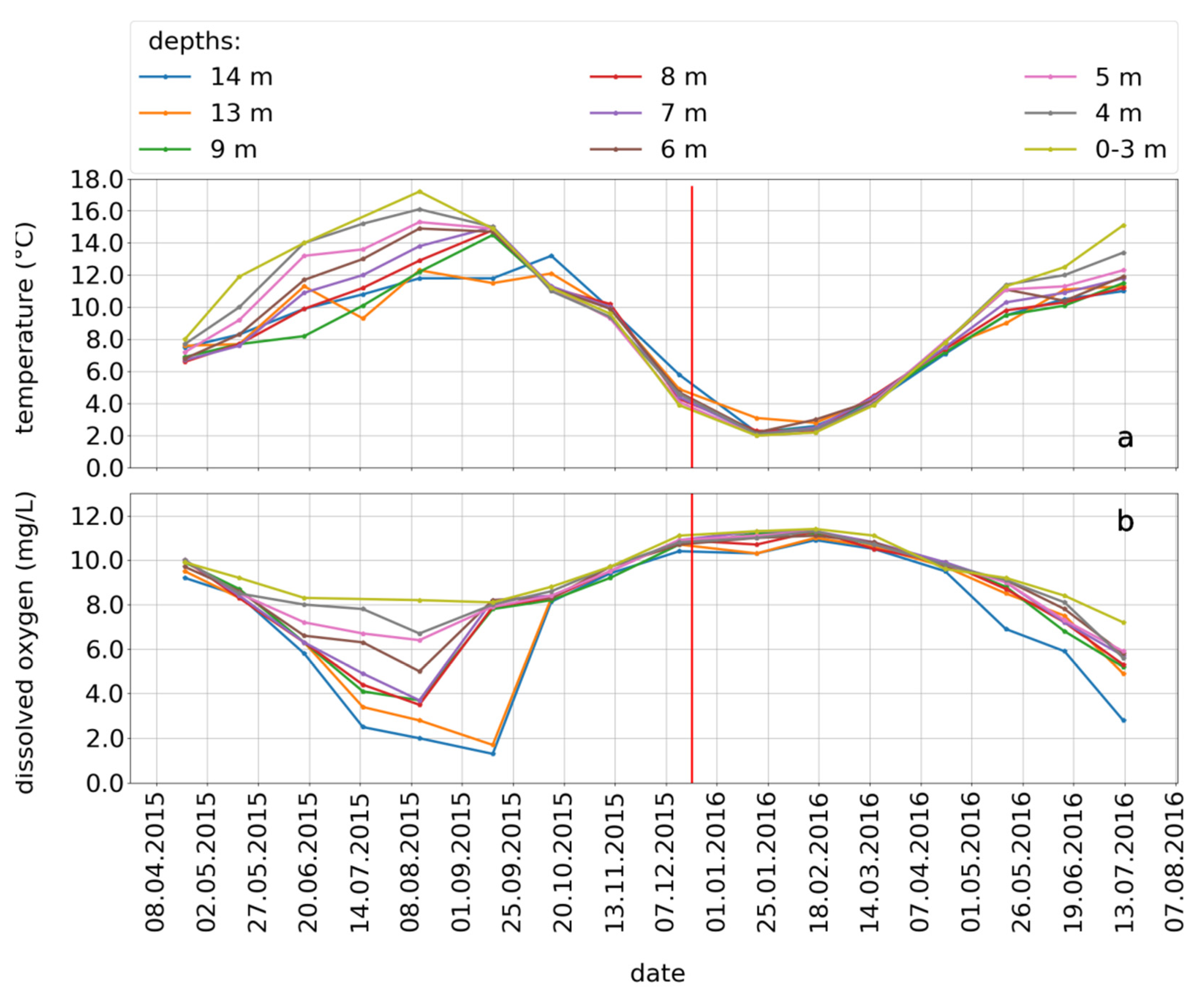
3.1. Seasonal Lake Stratification

In order to understand the seasonal and spatial differences of the DOM quality of the reservoir, the stratification in summer and the mixing conditions of the water body in autumn were investigated. Water temperature gradients were identified, confirming a stratification of the reservoir in late spring and summer (Figure 1a). There were either no or minor temperature differences detected between the different sampling depths in autumn and winter, evidencing the mixing of the water body. The temperature of the surface water was up to 17 °C in summer and about 2.5 °C in winter. In summer, the lowest temperatures observed were between 10 °C and 12.5 °C in the bottom water. A steeper temperature gradient in the reservoir was detected in summer 2015 compared to 2016 (Figure 1a). Dissolved oxygen (DO) behaved oppositely to water temperature (Figure 1b). In summer 2015, the concentration of DO in the lower layers of the reservoir decreased rapidly to values below 2 mg L⁻¹, which meant the water was hypoxic [56]. Considering the temperature (Figure 1a) and the DO (Figure 1b), the thickness of the hypolimnion was only about 2 m in September 2015. Between September and October 2015, the DO gradients disappeared due to mixing of the water body. Shortly before mixing, in September 2015, a large DO gradient between the bottom water and the overlaying water was observed. With increasing water depth, the DO depleted during the stratification period (Figure 1b). Seasonal and spatial differences of pH and the conductivity could also be observed according to lake stratification (Figure S1a,b).

In addition, stratification of the water body could also be observed by looking at the iron (Fe) and manganese (Mn) concentrations (Figure S3). During spring 2015, the iron concentration decreased slightly, whereas manganese concentrations were close to constant. In summer, the concentration of iron and manganese noticeably increased in the lake’s bottom water, whereas in upper layers, nearly no change was observed. This concentration gradient near the lake bottom disappeared in October after mixing, resulting in a slight increase of both Mn and Fe concentrations in the lake compared to spring. In February 2016, the concentrations decreased again.

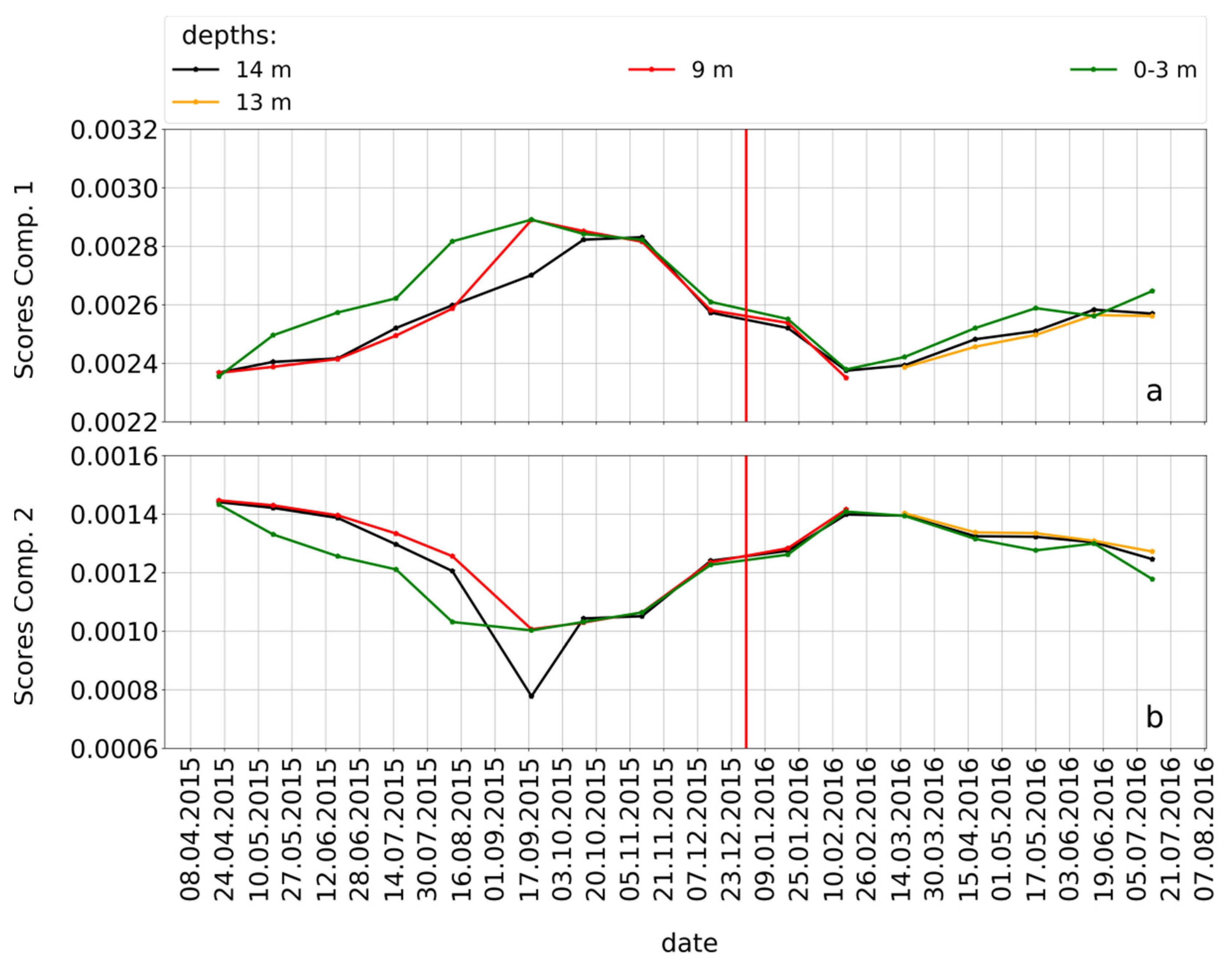
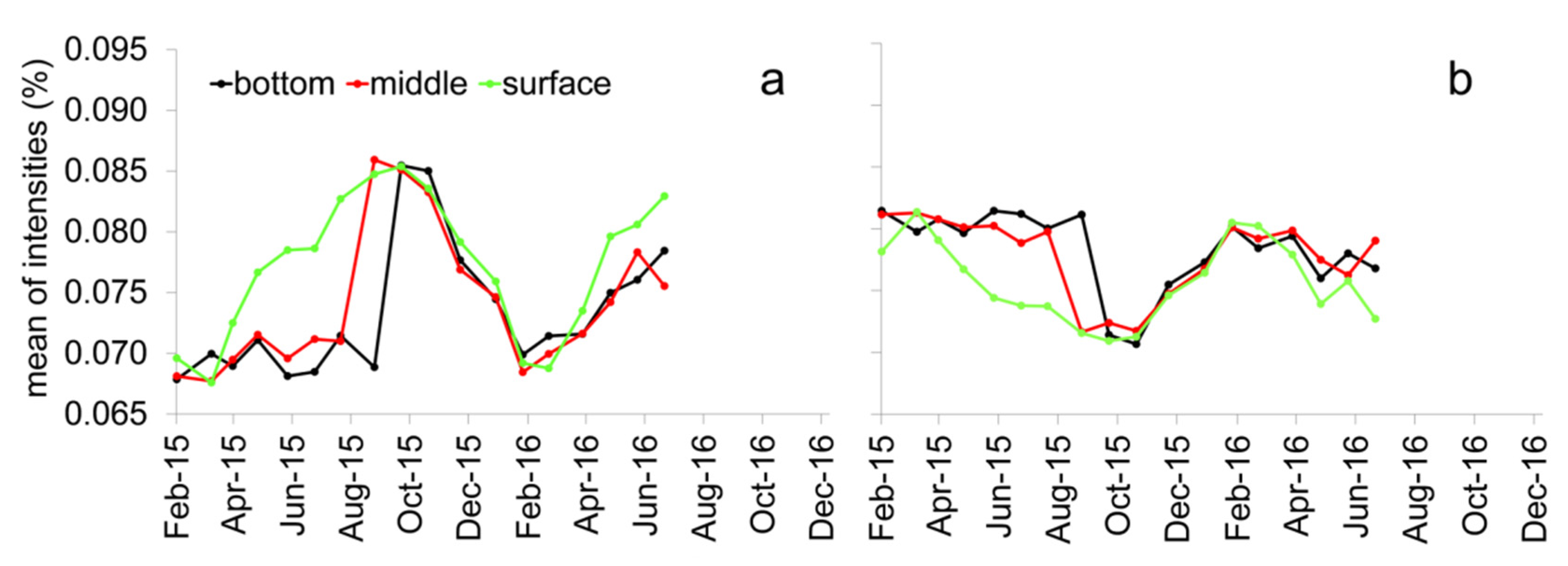
3.2. Seasonality of the PARAFAC Components within the Muldenberg Reservoir

To study the seasonality of the fDOM, monthly EEMs were measured over the whole sampling period. The evaluation of the EEMs showed that the fluorescence data were influenced by stratification and complete mixing within the Muldenberg reservoir (Figures S5 and S6). In summer (June 2015), the fluorescence difference was about 100 A.U. between the surface water and the layer 5 m below. However, in winter (December 2015), no differences were observed between the depths. To better investigate the seasonal behavior of the fDOM components, a PARAFAC analysis was performed. The PARAFAC model could be described by two calculated PARAFAC components (Figure S7). The PARAFAC components described 65% of the total model. The missing percentage indicated a third component which, however, could not be conclusively calculated. One reason might be the homogeneous distribution of the fDOM within the drinking-water reservoir.

For the characterization of the PARAFAC components, we used the emission and excitation loadings of the two components (Figure S8). The blue curve describes the first component, and the green the second. The emission maximum of the first component was 420 nm, and that of the second PARAFAC component was about 480 nm. The excitation maxima were 250 and 310 nm (first component) and 260 and 370 nm (second component), respectively. These PARAFAC components were humic-like and were also were detected in the pre-dams of the Muldenberg reservoir [23]. With regard to the study area, a protein-like fluorescence was not detected.

To study the behavior or distribution of the detected PARAFAC components, the scores were plotted over the sampling period for the relevant depths (Figure 2). The results showed that the two PARAFAC components had opposite seasonal and vertical behavior, with good resolution of the differences.

PARAFAC component 1 increased at all depths from April to September 2015, then decreased until February 2016, and increased again until July 2016 (Figure 2a). During spring and summer 2015, the loading of component 1 was higher at the lake surface compared to the lake bottom. In 2016, this effect was less distinct but still visible. This component may serve as an indicator for radiation-induced photochemical reactions and/or biological processes that produced fDOM starting in spring in both the mixed water body and the upper layer during stratification.

PARAFAC component 2 showed the opposite behavior compared to component 1 (Figure 2b). From April 2015 to August 2015, its loading was lower at the lake surface compared to the lake bottom. In September 2015, the loadings of both components were lower at the lake bottom compared to the lake surface. The low score of PARAFAC component 2 in September 2015 at the lake bottom cannot currently be explained. In any case, it was accompanied by elevated iron and manganese concentrations. Since the isomeric structures of DOM are still unknown, a more detailed discussion of this issue is not indicated. During autumn and winter, no loading difference as function of depth was found between both components (Figure 2a,b). This means that this component was characterized by the radiation-degraded fDOM components. We concluded that component 2 must have been partially consumed in the epilimnion, whereas component 1 must have been partially produced. The supply of component 1 from the catchment area seemed to increase from spring to late summer, and then to decrease from the autumn to winter. Component 2 seemed to increase after completing the stratification period.

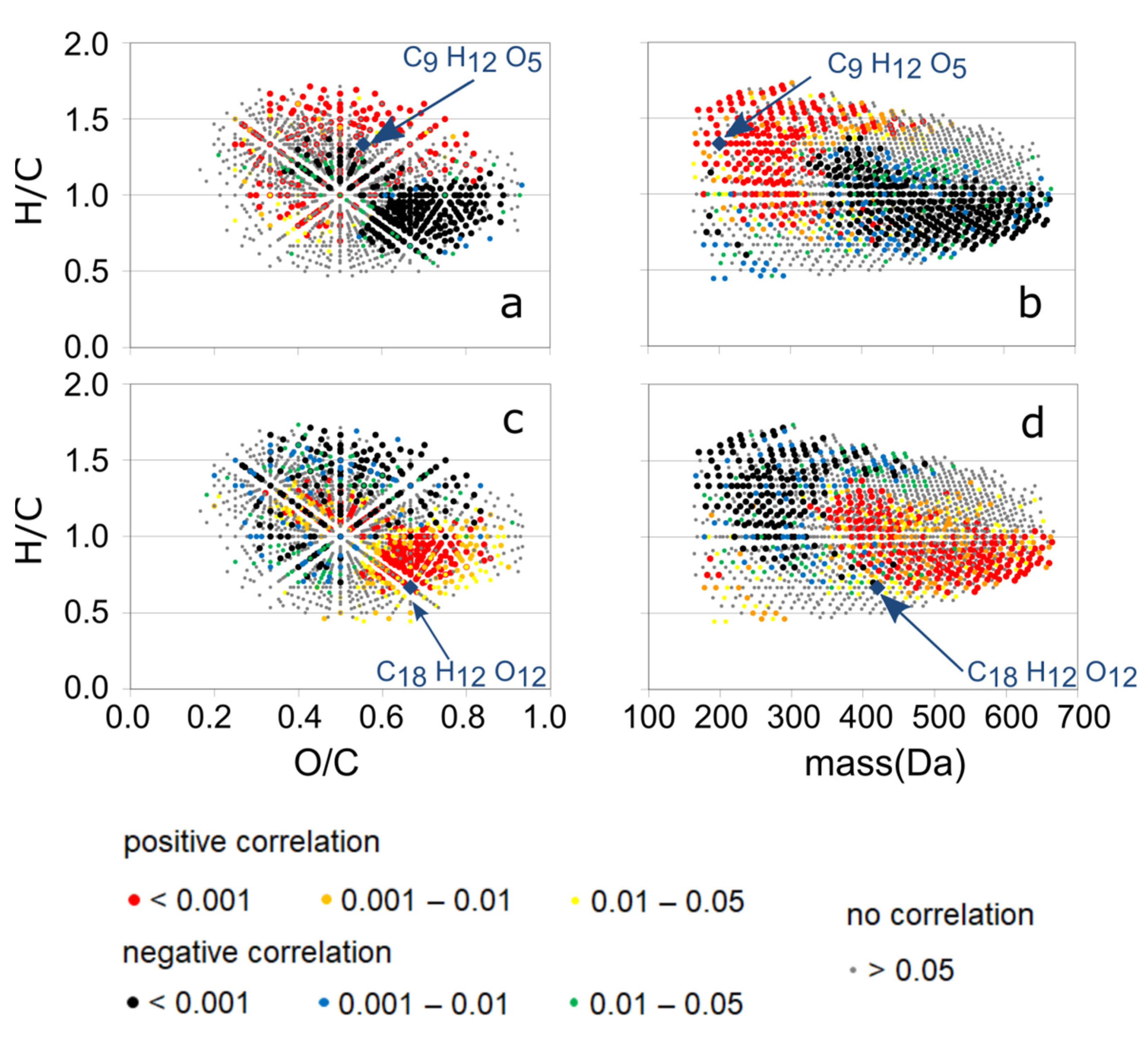
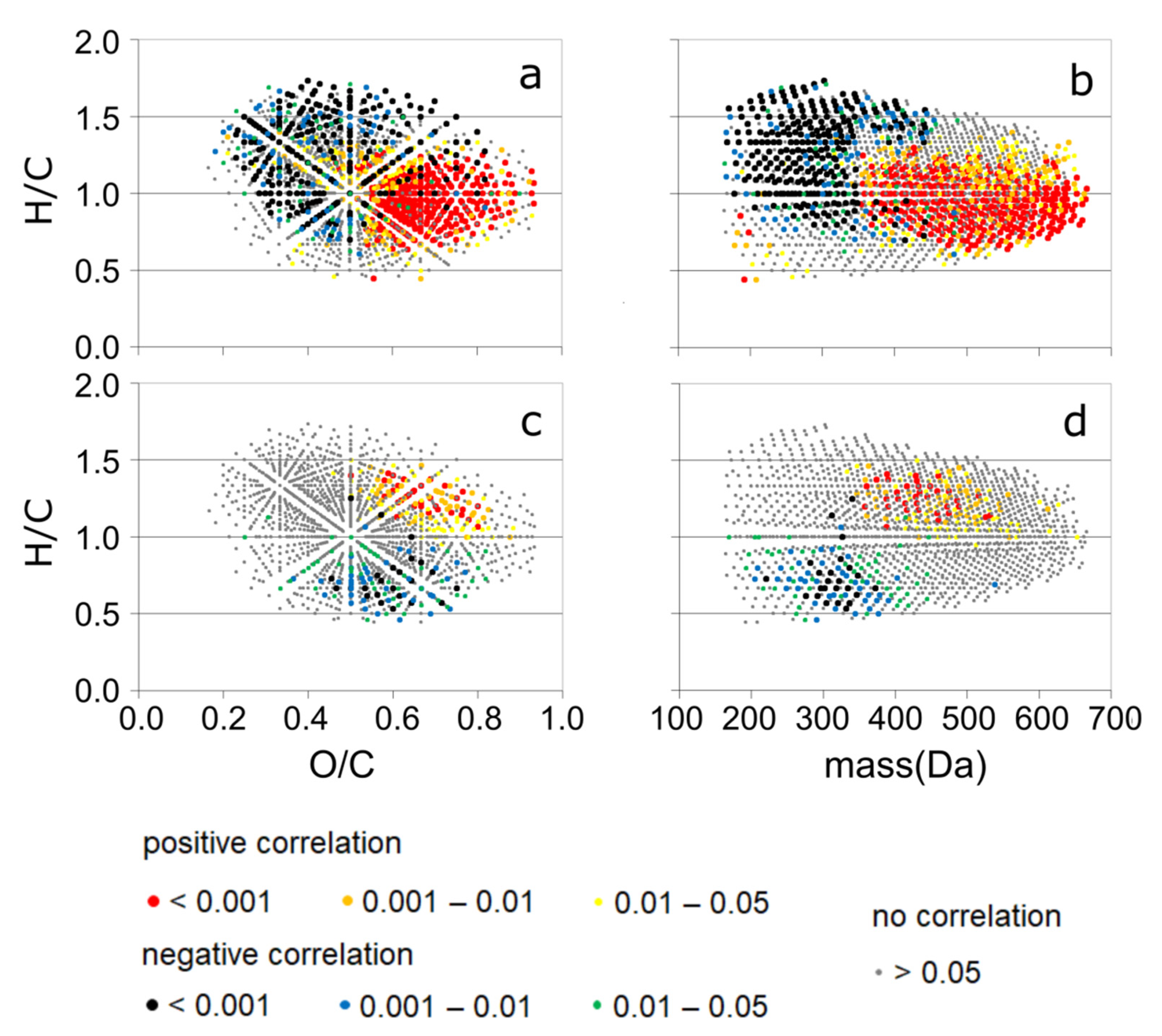
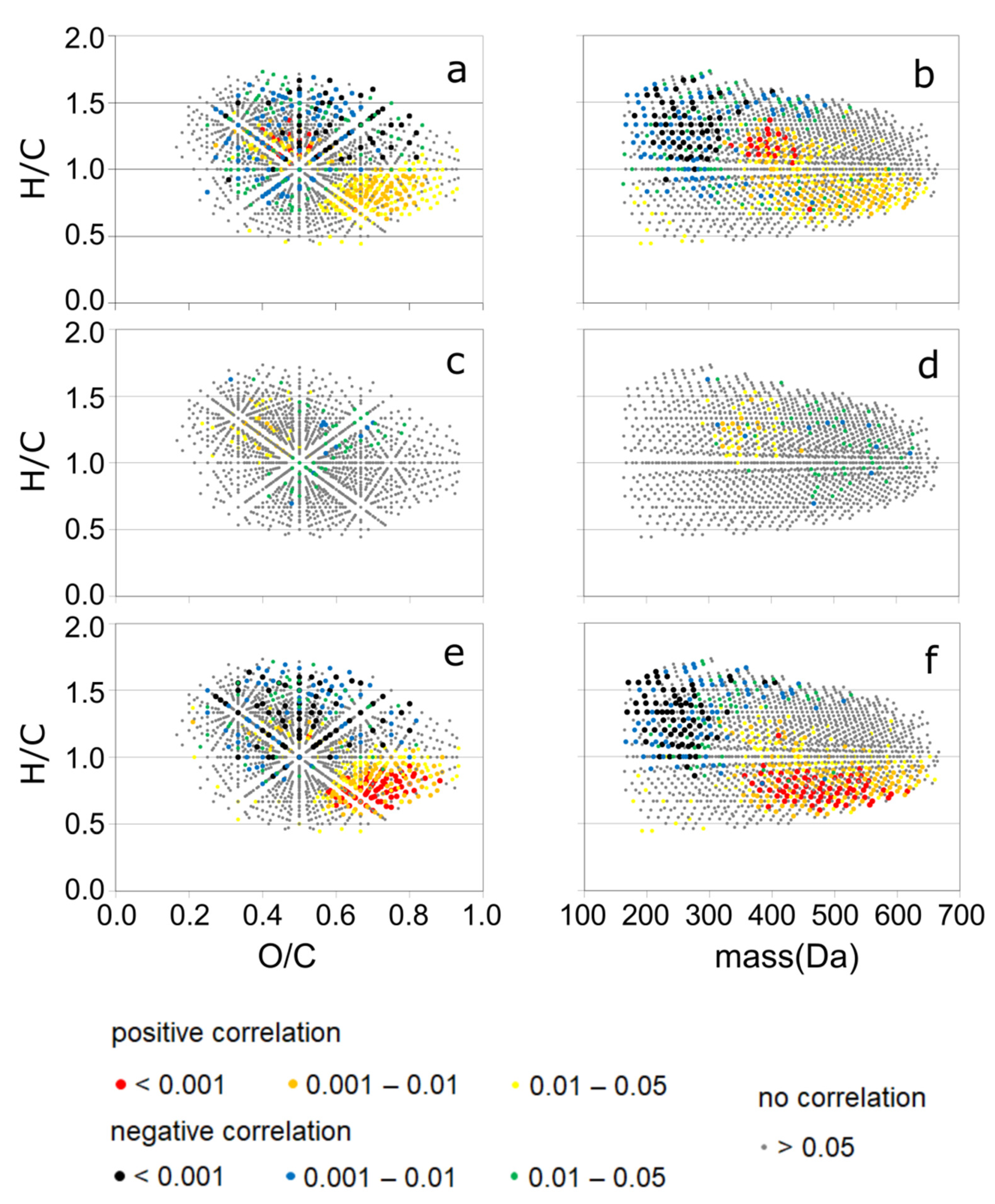
3.3. Detailed Information about DOM Seasonality from Spearman’s Rank Correlation of CHO-MF and the PARAFAC Components

In order to estimate the raw water quality based on 2D-fluorescence measurements, it was necessary to shed further light on the chemical characteristics of the DOM constituents related to the two identified PARAFAC components. For this purpose, all 54 samples were investigated by FTICR MS, which is a costly and laborious method. For correlation calculations, we only used the CHO-MF, because their abundance was dominant compared to others, like CHNO, CHOS, or CHNOS.

Based on these results, the chemistry of the PARAFAC components could be estimated by Spearman’s rank correlation to MF data from FTICR MS for a limited study period. Once the chemistry of the PARAFAC components has first been evaluated, the fluorescence spectrometry can then be used alone for predicting raw water quality. Figure 3 shows the Spearman’s rank correlation of the relative MF intensities as detected by FTICR MS, and the two calculated PARAFAC components of all CHO-MF in 48 samples (where results from fluorescence spectroscopy were available for correlation calculations, see Table S1). The classification of the Spearman’s rank correlation coefficients was carried out according to the uncertainties (p < 0.001, 0.001 < p < 0.01, 0.01 < p < 0.05, and p > 0.05).

The correlations between the loadings of PARAFAC component 1 (Figure 3a,b) and total common present MF intensities is reversely distributed with positively and negatively correlated MFs compared to PARAFAC component 2 (Figure 3c,d). The positively correlated MFs had an H/C ratio between 0.5 and 1.7, and an O/C ratio between 0.2 and 0.8. In comparison to the PARAFAC component 2, the first component was characterized by positive correlations with low-molecular-weight MFs <400 Da. The MFs correlated negatively to component 1 had higher masses >400 Da, mainly with MFs with O/C > 0.6 and H/C < 1.1. These MFs were mainly positively correlated to component 2. A small group of MFs with 300 Da < mass < 500 Da, 1 < H/C < 1.4, and 0.3 < O/C < 0.6 was also positively correlated with component 2. Positively correlated MFs were mainly linked with larger masses between 400 and 700 Da. The H/C ratio of those MFs was between 0.5 and 1, and the O/C ratio was between 0.6 and 0.9.

By evaluating the rank correlation, the following chemistry specifications could be identified for the PARAFAC components: PARAFAC component 1 represented relative aliphatic MFs with lower molecular weights, and component 2 represented more aromatic, higher-oxygenated and higher-molecular-weight MFs. The reactivity might explain the seasonality effects during stratification of the reservoir.

In order to investigate seasonality of MF with a highly positive (product group, Figure 4) or highly negative (degraded group, Figure S12) correlation with the two PARAFAC components, the mean of the relative intensities (RIs) of the MFs were plotted over the sampling time period (Figure 4). MF (product group) with a highly positively correlation with PARAFAC component 1 (Figure 4a) showed an increase from April to October 2015 in the surface layer. The mean RI of the middle and bottom depths increased in August and September 2015 respectively, and decreased again after mixing in October and November 2015. The same distribution was observed for the MF with a negatively correlation with PARAFAC component 2 (Figure S12b). A slightly higher mean RI of PARAFAC component 2 in comparison to component 1 was observed. Notably, PARAFAC component 2 had an overall lower score than component 1 (Figure 3). It could be concluded that PARAFAC component 2 had a lower score, but the highly correlated MFs had a higher mean RI. The degraded group showed the opposite distribution of the product group. MF with a highly positive correlation with PARAFAC component 2 decreased from April 2015 to August 2015, and increased in November 2015 (Figure 4b) in the surface layer. In winter 2015/2016, the mean RI increased again. The mean RI of the middle and bottom layers decreased during summer stratification and increased with the mean RI of the surface layer in October 2015 (Figure 4b).

In the course of this investigation, we obtained information regarding the seasonality of the MFs in the reservoir that were highly correlated with the detected PARAFAC components. Based on this information, it may be concluded that relatively aliphatic MFs with low molecular weights had higher intensities during stratification, and were mainly represented on the surface. The aromatic structures with higher oxygen content and higher molecular weights decreased in summer. The decrease was first present on the surface, and then also in the lower levels.

To elucidate the potential reactivity, the seasonality of two different MFs was selected, as described in the next section.

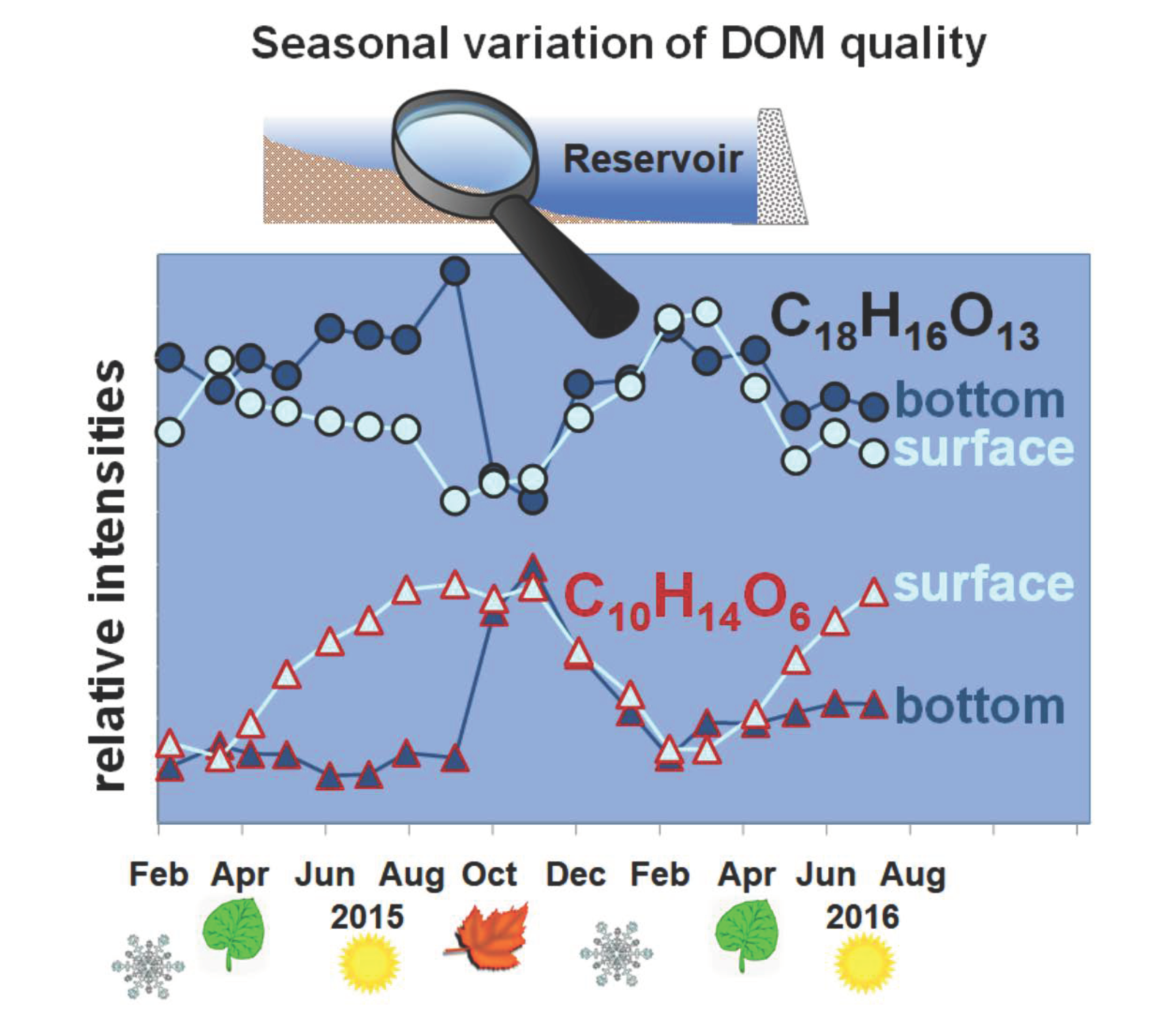
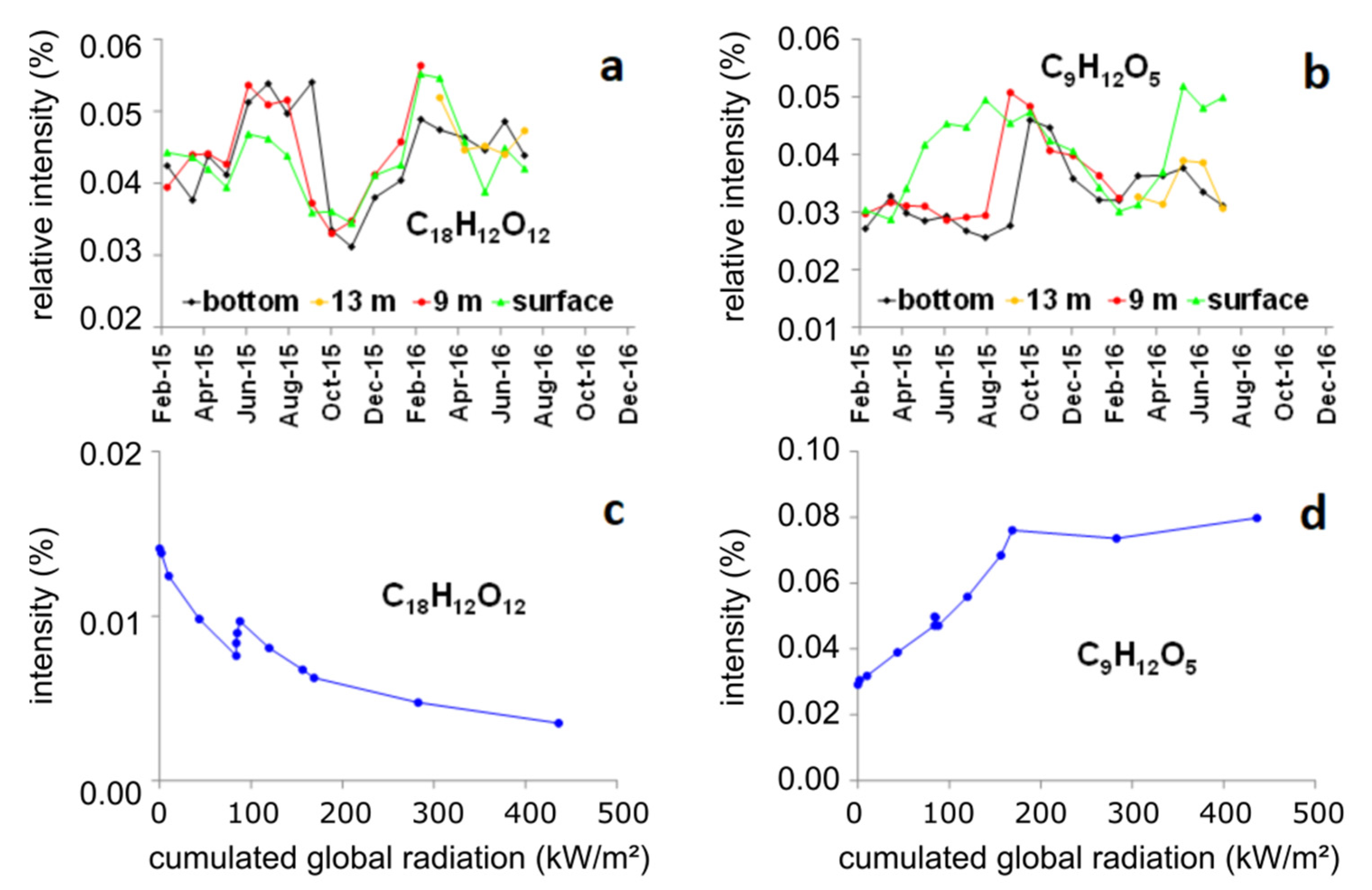
3.4. Detailed Analysis of Two Exemplary MFs and Combination with Reactivity Data from the Literature

As explained in the last section, MFs with different seasonalities were identified. In order to understand the observed seasonal behavior, we selected some MFs whose biogeochemical reactivity has been already discussed in the literature [5,30]. Firstly, the rather opposite seasonal behavior of C₉H₁₂O₅ and C₁₈H₁₂O₁₂ shall be debated. The MF C₉H₁₂O₅ represents compounds correlating positively with PARAFAC component 1, while MF C₁₈H₁₂O₁₂ represents those correlating positively with PARAFAC component 2.

The component C₉H₁₂O₅ (Figure 5b) was characterized by a continuous increase from April to September 2015 at the lake surface, whereas at the lake bottom, its relative intensity (RI) remained mostly unchanged. The RI at the bottom rose to the level of that of the surface water at the end of stratification in October 2015. Its RI was higher in the epilimnion compared to the hypolimnion during the summer months. This can be interpreted as partial production of this compound in the epilimnion. The same component showed similar seasonal and spatial behavior in the Rappbode pre-dam [30]. At this location, the intensity of C₉H₁₂O₅ also increased at the lake surface (epilimnion) during the summer. A considerable RI difference was observed between the epilimnion and hypolimnion in comparison to the Muldenberg Reservoir. The Rappbode Reservoir is about five times larger than the Muldenberg Reservoir.

C₁₈H₁₂O₁₂ showed the opposite behavior (Figure 5a). Its RI was nearly constant at the lake bottom from June to September 2015 (after an increase from May to June) (Figure 5a). Its RI fell during that period at the lake surface, resulting in maximum RI difference, in September 2015, between the lake bottom and lake surface. After lake stratification ended in October 2015 (mixing of epilimnion water with hypolimnion water), the RI of C₁₈H₁₂O₁₂ reached its seasonal minimum, and subsequently increased at all depths until February 2016. C₁₈H₁₂O₁₂ was evidently consumed in the epilimnion.

The reactivities, production of C₉H₁₂O₅, and consumption of C₁₈H₁₂O₁₂ in the epilimnion can be explained by the results of a former study. Inflow water to a pre-dam of the Muldenberg Reservoir was irradiated with natural sunlight in order to investigate the photochemical reaction of the DOM [5]. The component C₁₈H₁₂O₁₂ (Figure 5c) was detected as a photo-degraded compound, and C₉H₁₂O₅ (Figure 5d) as photo product.

In summary, PARAFAC component 1 was an indicator for the photo-degraded fraction of the humic material (newly formed). The second PARAFAC component behaved like material that was of terrestrial and allochthonous (strongly humic-like) origin, and underwent photochemical degradation like the C₁₈H₁₂O₁₂. Component 2 had a higher concentration above ground and was also more aromatic due to the correlation to MFs with low H/C values (Figure 5a,c). The quotient of PARAFAC component 1/PARAFAC component 2 seemed suitable to evaluate the degree of DOM photo transformation in the reservoir water.

However, the issue of the seasonal behavior during winter months remains to be explained.

On the one hand, photo products such as C₉H₁₂O₅ were evidently depleted from October 2015 to February 2016. They were increasingly exported from the reservoir downstream part of the Mulde River, and were no longer produced in the reservoir, or the pre-dam as inflowing water, due to the winter-related reduced intensity of solar radiation (according to PARAFAC component 1 in Figure 2a). In spring 2016, the RI increase was observed at the surface again for the compound C₉H₁₂O₅.

On the other hand, components like C₁₈H₁₂O₁₂, which easily undergo photo-degradation, show no further signs of depletion as solar radiation intensity decreased with the beginning of winter.

Another effect was observed which potentially originates from hypoxia and has been discussed in Section 3.1. Several oxygen-rich and relatively unsaturated components such as C₁₇H₁₈O₁₄ showed similar profiles to iron and manganese during a short period in the summer and autumn of 2015 (Figure S2, component; Figure S3, iron and manganese). They had high RIs at the lake bottom in September 2015. The difference in RIs between the surface and bottom samples (Figure S2) on the sampling date in September as DO reached its minimum in the bottom water, is remarkable. After stratification finished in October, no further RI difference of such a distinct level was observed. This can be explained by the release of carboxylate-rich components under hypoxic conditions after reduction of ferric iron minerals the former having adsorbed these components by complexation. The potential release of oxygen-rich and relatively unsaturated components from sediments under anoxic conditions already has been thoroughly discussed by Dadi et al. [6].

Summarizing the present main outcomes, with the rank correlation performed between MF intersample ranks and, e.g., PARAFAC components, such MFs with potential seasonal and vertical changes of relative intensities could be easily recognized. The two discussed sunlight-related MFs were selected to demonstrate the seasonal and vertical fluctuations within the Muldenberg reservoir. Using these two MF examples, the observations were combined to explain the correlations and variances.

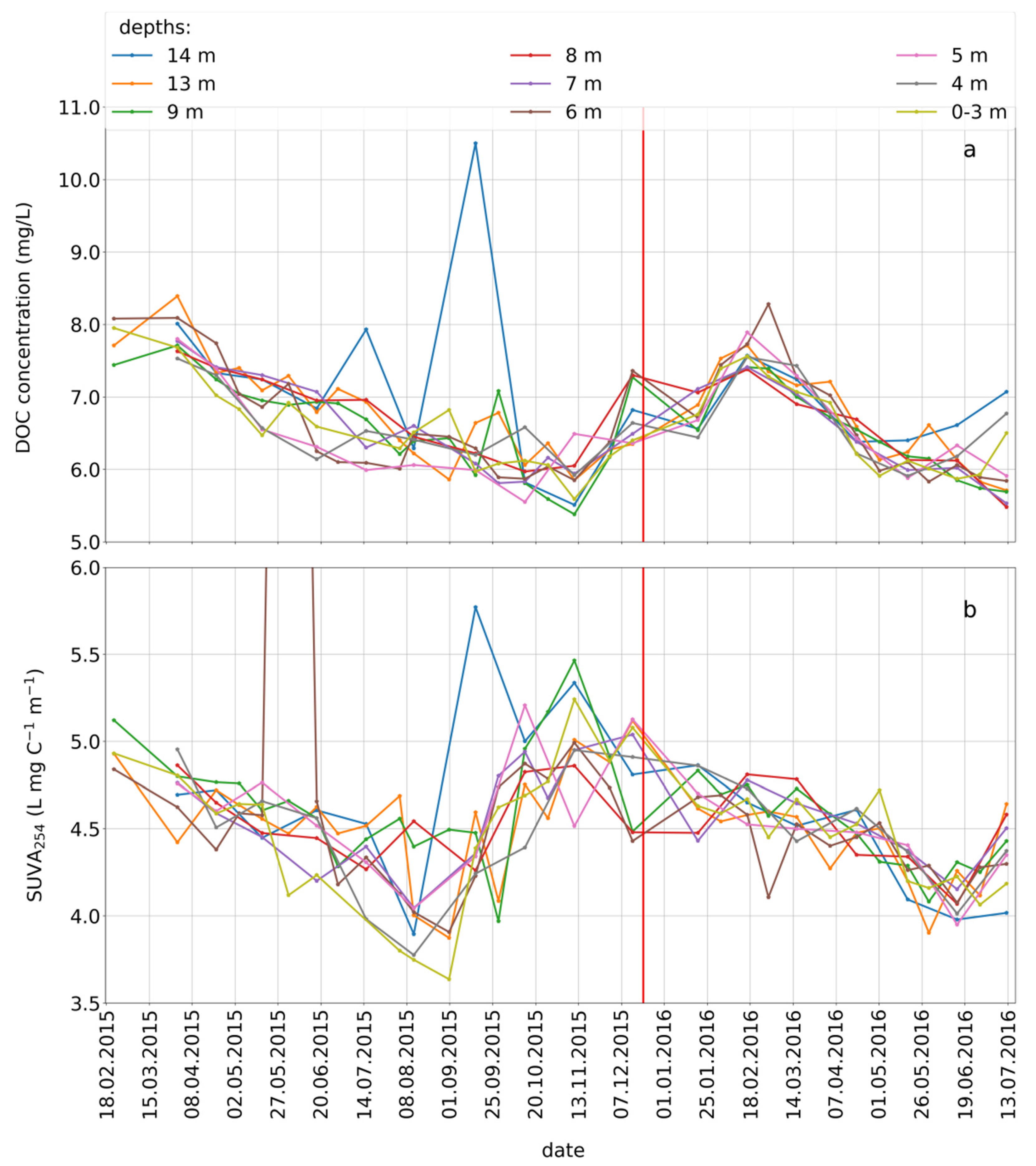
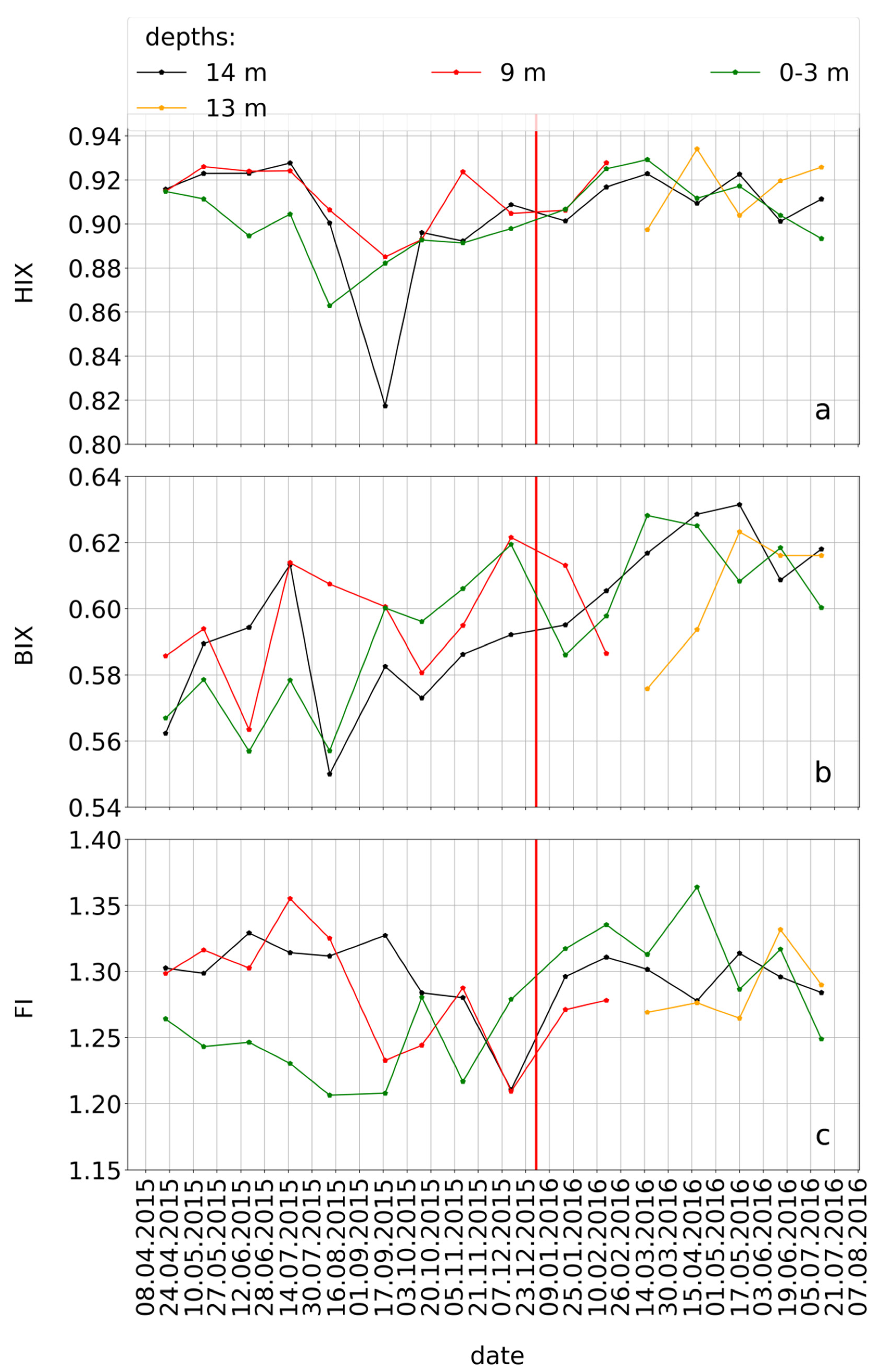
3.5. Seasonal Variations of the Concomitant Parameters

The DOC concentrations depleted slightly from spring to summer 2015 (showing the same trend as in 2016), with no uniform trend to establish distinct gradients as a function of water depth. Regarding the raw water quality, DOC does not seem to be a very meaningful parameter. The highest DOC concentrations were observed between 7 and 8 mg L⁻¹ at all depths, in winter 2015 and 2016 (Figure 6a, Table S1). The low DO concentration and the shallow hypolimnion layer of only 1 or 2 m (Figure 1b, Table S1) explain the high DOC concentration in September 2015. Therefore, as mentioned in the preceding section, mostly polyphenol-like components could be released from sediment into the water body through iron reduction. The same distribution or “peak” was observed with the MF C₁₇H₁₈O₁₄ (Figure S2) and the iron concentration (Figure S3, Table S1). If the volume of the hypolimnion was very small at this time, small DOC inputs from the sediment could lead to visible increases in concentration.

The SUVA₂₅₄ did not show vertical differences, and was between 4 and 6 L mgC⁻¹ m⁻¹ over the whole sampling time (Figure 6b, Table S1). The value of 13.6 L mgC⁻¹ m⁻¹ in May 2015 must have arisen due to the UV value at 254 nm. This cannot be explained.It is defined as an extreme value and may be an outlier. SUVA is often used as a proxy for aromaticity and for humic-rich and colored water. The fluctuations in SUVA (Figure 6b) were not significant, and were similar to other lakes [57]. In this reservoir, SUVA monitoring alone as a function of time and depth appears to be insufficient to describe the DOM quality for raw-water-quality evaluation.

Further resolution may be provided by the fluorescence indices (Figure 7, Table S1). The HIX and FI showed more seasonal differences as a function of depths compared to the BIX. In spring and summer 2015 and in summer 2016, the largest differences between surface and bottom water were observed for the HIX, with the higher levels at the bottom. From spring to fall 2015, an overall depletion from more than 0.92 to 0.88 occurred. In September 2015, the HIX values decreased from 0.9 to 0.82 at the bottom. The BIX did not show as intensive a variation as the SUVA. The values ranged between 0.55 and 0.63. In 2016, the BIX values were higher than in 2015.

The FI of bottom water was higher than that of surface water in 2015. The FI of the surface water was between 1.2 and 1.25 from spring to summer 2015, and the FI of the bottom water was up to 1.3 (Table S1). From September 2015 to December 2015, the water mixed, as did the FI values between the depths. In 2016, the distribution changed and all values at nearly all depths were between 1.25 and 1.35. Photolysis processes were observed to result in a decrease of the FI during summer in the surface water [57].

3.6. Seasonality of the Concomitant Parameters Based on the Spearman’s Rank Correlation with the CHO-MF

To link seasonality behavior between the different observed and calculated parameters, we have calculated the Spearman’s rank correlation coefficients (

Table 1. Spearman’s correlation coefficient matrix of the calculated ranks of observed and calculated parameters. Values in bold indicate significant correlation.

	DOC	SUVA	HIX	BIX	FI	Comp1	Comp2
DOC	1
SUVA	0.021	1
HIX	0.421	−0.005	1
BIX	−0.065	−0.160	0.260	1
FI	0.357	−0.059	0.347	0.134	1
Comp1	−0.677	−0.034	−0.719	−0.060	−0.437	1
Comp2	0.583	−0.035	0.728	0.093	0.467	−0.970	1

).

PARAFAC component 2 and HIX were highly positively correlated (Table 1). PARAFAC component 2 was positively related to the DOC (Table 1). The other fluorescence indices and SUVA were less appropriate due to their weaker correlations with PARAFAC component 2.

The correlation distribution in van Krevelen diagrams was completely different for the SUVA (Figure 8c,d) and BIX (Figure 9c,d). Positively correlated MFs in the SUVA diagram had H/C ratios between 1 and 1.5 and a molecular weight > 400 Da. The O/C ratio mainly ranged between 0.5 and 0.9, whereas the negatively correlated MFs were found to be 0.4 < O/C < 0.6. Negatively correlated MFs showed H/C between 0.5 and 1 and lower masses <400 Da. A low number of MFs were found to be significantly correlated to BIX in comparison to the other correlated parameters. MFs correlated positively to DOC had somewhat larger H/C values compared to those correlated to HIX, FI, and PARAFAC component 2 (Figure 8a,b as well as Figure 8e,f and Figure 2). A positive correlation of HIX and the second PARAFAC component (Table 1) suggested that the carbon structures of this component were related to aromatic molecules [58].

Finally, it can be stated that the PARAFAC components allowed for a more detailed insights and provided more information in comparison to the SUVA or BIX, as these parameters had no significant correlation with any of these components (Figure 2, Figure 8c,d as well as Figure 9c,d, and Table 1). FI and BIX were mainly negatively correlated to HIX [28] but, in the Muldenberg reservoir, the HIX and FI had similar distributions of correlations with MF within the van Krevelen diagram (Figure 8a,b,e,f).

Overall, correlation calculations and inclusion molecular information from the FTICR MS (MF and intensity) provided more detailed information on the real DOM quality fluctuations than the bulk parameters alone, as specified in Table 1.

3.7. Outlook in Terms of Relevance to the Waterworks

In a previous study [30], different MFs with specific characteristics for drinking-water treatment were observed. The rank correlation coefficients of selected MFs were calculated and compared (

Table 2. Selected molecular formulas (MFs), their molecular masses, reactivities (Chla: correlation to chlorophyll a; Rad: correlation to radiation; and +/−/0: positive/negative/no correlation), and rank correlation coefficients between photo products or photo-degraded compounds and the scores of the PARAFAC components as well as the fluorescence indices HIX, BIX, and the DOC. Chla⁺ Rad⁺ are photo products, Chla⁻ Rad⁻ are photo-degraded compounds, Chla⁺ Rad⁰ are microbial products, and Rad- are also photo degraded compounds [30], the byproducts of which are potential precursors for disinfection byproducts [13,14,15].

MF	Mass	Byprod. Precursor	Reactivity	Rank Correlation Coefficient
				Score 1	Score 2	HIX	BIX	DOC
C9H12O5	200.068	-	Chla+ Rad +	+0.62	−0.56	−0.68	0	−0.69
C18H12O12	420.033	-	Rad−	−0.54	+0.48	+0.63	+0.20	+0.34
C9H12O6	216.063	Yes	Chla+ Rad+	+0.64	−0.59	−0.69	−0.02	−0.67
C10H14O7	246.074	Yes	Chla+ Rad+	+0.72	−0.67	−0.72	−0.05	−0.68
C16H12O10	364.043	Yes	Chla− Rad−	−0.34	+0.29	+0.35	−0.003	+0.24
C14H16O8	312.085	Yes	Chla+ Rad0	+0.27	−0.90	−0.94	−0.51	−0.97
C19H28O8	384.178	Yes	Chla+ Rad0	+0.26	−0.23	−0.12	+0.45	−0.36
C18H14O12	422.049	-	Chla− Rad−	−0.65	+0.55	+0.63	+0.04	+0.58
C18H14O13	438.043	-	Rad−	−0.61	+0.52	+0.64	+0.22	+0.54
C18H14O14	454.038	-	-	−0.57	+0.47	+0.63	+0.22	+0.53

) to decide if the additional information obtained from the fluorescence indices, the PARAFAC modeling, and the results of the FTICR MS measurements, were useful with respect to the waterworks. The information that MFs were found to be potential precursors of disinfection byproducts was contrasted with the above-mentioned parameters. The relative intensities over the sampling period in the Muldenberg Reservoir (present study), and their intensities in a photodegradation experiment (Wilske et al. 2020) [5], are shown in Figures S10 and S11.

Highly unsaturated and oxygen-rich compounds, as in the case of the discussed photo-degraded compound C₁₈H₁₂O₁₂, may be coagulated with iron or aluminum salts due to their potential phenol- and/or carboxylate-rich moieties. By using coagulation or other water-treatment processes, like aluminum coagulation or chlorination, up to 50% of the humic-like components were mostly removed [59]. It was shown that the removal efficiency (coagulation) increased with decreasing H/C in a series of MFs having the same O/C [10]. In the series C₁₈H₁₀O₁₂, C₁₈H₁₂O₁₂, C₁₈H₁₄O₁₂, C₁₈H₁₆O₁₂, C₁₈H₁₈O₁₂, C₁₈H₂₀O₁₂, C₁₈H₂₂O₁₂, C₁₈H₂₄O₁₂, the first two members would have the highest coagulation potential. Evidently, the behavior of such DOM constituents can be followed using PARAFAC modeling, as shown by the correlation with PARAFAC component 2. This meant that a proxy for removal efficiency of such humic substances was available. In addition to the removal of humic-like substances, the formation of disinfection byproducts, is of course a crucial issue. PARAFAC component 1 evidently was a proxy for another class of humic-like substances that comprises a large number of photo products. As with C₉H₁₂O₅, C₉H₁₂O₆, or C₁₀H₁₄O₇, such DOM constituents were reported to be potential precursors of disinfection byproducts (Table 2) [13,14,15,55]. This issue might be addressed in the future.

4. Limitations

FTICR MS analysis provided by far the highest analytical resolution addressing DOM quality to date. However, it may be suggested that only part of the bulk DOM was detectable by FTICR MS due to the following reasons. Only the SPE-DOM was detectable. Components that were not adsorbed on PPL cartridges or those which were too strongly adsorbed and could not be eluted by methanol were not detectable [41]. Using the negative electrospray ionization technique, only ionizable components could be detected in the mass spectrometer. Only low-molecular-weight molecules (<800 Da) were considered. Nevertheless, at present, there is no analytical technique to simultaneously overcome the demand on resolution and the completeness of the DOM fraction. A more detailed explanation of the limitations was described in [30].

5. Conclusions

According to our hypothesis, the seasonal change of DOM quality was detected in a reservoir dominated by terrestrial material (humic-like and colored), which could be explained mainly by photochemical transformations. Combining FTICR MS results with EEMs through intersample rank correlations showed that photochemical processes destroyed higher-molecular-weight fluorophore substances and formed smaller fluorophore molecules.

Differences in the distribution of fluorescent components between the epilimnion and hypolimnion were observed, the importance of which for the estimation of specific DOM molecular sizes, was confirmed by correlation with FTICR MS data. A proxy for DOM molecular weight might be one of the decision parameters for drinking-water treatment.

To ensure that the waterworks can use the detailed information generated by combining PARAFAC and FTICR MS for raw-drinking-water treatment, seasonal measurements should be performed, not only in raw, but also in drinking water. It would be important to determine how the two PARAFAC components behave, and whether they affect DOM removal positively or negatively. In terms of future choice of water depth for raw water abstraction, the online sensor provides additional information about molecular structures and the photo reactions in the reservoir.

References

1. Xu, J.; Morris, P.J.; Liu, J.; Ledesma, J.L.J.; Holden, J. Increased Dissolved Organic Carbon Concentrations in Peat-Fed UK Water Supplies Under Future Climate and Sulfate Deposition Scenarios. Water Resour. Res. 2020, 56, e2019WR025592. [Google Scholar] [CrossRef] [Green Version]
2. Morling, K.; Herzsprung, P.; Kamjunke, N. Discharge determines production of, decomposition of and quality changes in dissolved organic carbon in pre-dams of drinking water reservoirs. Sci. Total Environ. 2017, 577, 329–339. [Google Scholar] [CrossRef]
3. Herzsprung, P.; von Tumpling, W.; Hertkorn, N.; Harir, M.; Buttner, O.; Bravidor, J.; Friese, K.; Schmitt-Kopplin, P. Variations of DOM Quality in Inflows of a Drinking Water Reservoir: Linking of van Krevelen Diagrams with EEMF Spectra by Rank Correlation. Environ. Sci. Technol. 2012, 46, 5511–5518. [Google Scholar] [CrossRef] [PubMed]
4. Kraus, T.E.C.; Bergamaschi, B.A.; Hernes, P.J.; Doctor, D.; Kendall, C.; Downing, B.D.; Losee, R.F. How reservoirs alter drinking water quality: Organic matter sources, sinks, and transformations. Lake Reserv. Manag. 2011, 27, 205–219. [Google Scholar] [CrossRef] [Green Version]
5. Wilske, C.; Herzsprung, P.; Lechtenfeld, O.J.; Kamjunke, N.; von Tumpling, W. Photochemically Induced Changes of Dissolved Organic Matter in a Humic-Rich and Forested Stream. Water 2020, 12, 331. [Google Scholar] [CrossRef] [Green Version]
6. Dadi, T.; Harir, M.; Hertkorn, N.; Koschorreck, M.; Schmitt-Kopplin, P.; Herzsprung, P. Redox Conditions Affect Dissolved Organic Carbon Quality in Stratified Freshwaters. Environ. Sci. Technol. 2017, 51, 13705–13713. [Google Scholar] [CrossRef]
7. Bracchini, L.; Dattilo, A.M.; Hull, V.; Loiselle, S.A.; Nannicini, L.; Picchi, M.P.; Ricci, M.; Santinelli, C.; Seritti, A.; Tognazzi, A.; et al. Spatial and seasonal changes in optical properties of autochthonous and allochthonous chromophoric dissolved organic matter in a stratified mountain lake. Photochem. Photobiol. Sci. 2010, 9, 304–314. [Google Scholar] [CrossRef] [PubMed]
8. Andersson, A.; Lavonen, E.; Harir, M.; Gonsior, M.; Hertkorn, N.; Schmitt-Kopplin, P.; Kylin, H.; Bastviken, D. Selective removal of natural organic matter during drinking water production changes the composition of disinfection by-products. Environ. Sci. Water Res. Technol. 2020, 6, 779–794. [Google Scholar] [CrossRef]
9. Niquette, P.; Monette, F.; Azzouz, A.; Hausler, R. Impacts of substituting aluminum-based coagulants in drinking water treatment. Water Qual. Res. J. Can. 2004, 39, 303–310. [Google Scholar] [CrossRef]
10. Raeke, J.; Lechtenfeld, O.J.; Tittel, J.; Oosterwoud, M.R.; Bornmann, K.; Reemtsma, T. Linking the mobilization of dissolved organic matter in catchments and its removal in drinking water treatment to its molecular characteristics. Water Res. 2017, 113, 149–159. [Google Scholar] [CrossRef] [PubMed]
11. Awad, J.; van Leeuwen, J.; Chow, C.W.K.; Smernik, R.J.; Anderson, S.J.; Cox, J.W. Seasonal variation in the nature of DOM in a river and drinking water reservoir of a closed catchment. Environ. Pollut. 2017, 220, 788–796. [Google Scholar] [CrossRef]
12. Zhang, H.F.; Zhang, Y.H.; Shi, Q.; Ren, S.Y.; Yu, J.W.; Ji, F.; Luo, W.B.; Yang, M. Characterization of low molecular weight dissolved natural organic matter along the treatment trait of a waterworks using Fourier transform ion cyclotron resonance mass spectrometry. Water Res. 2012, 46, 5197–5204. [Google Scholar] [CrossRef]
13. Phungsai, P.; Kurisu, F.; Kasuga, I.; Furumai, H. Molecular characterization of low molecular weight dissolved organic matter in water reclamation processes using Orbitrap mass spectrometry. Water Res. 2016, 100, 526–536. [Google Scholar] [CrossRef] [PubMed] [Green Version]
14. Phungsai, P.; Kurisu, F.; Kasuga, I.; Furumai, H. Changes in Dissolved Organic Matter Composition and Disinfection Byproduct Precursors in Advanced Drinking Water Treatment Processes. Environ. Sci. Technol. 2018, 52, 3392–3401. [Google Scholar] [CrossRef]
15. Phungsai, P.; Kurisu, F.; Kasuga, I.; Furumai, H. Molecular characteristics of dissolved organic matter transformed by O3 and O3/H2O2 treatments and the effects on formation of unknown disinfection by-products. Water Res. 2019, 159, 214–222. [Google Scholar] [CrossRef] [PubMed]
16. ISO. DIN EN 1484: 2019-04. Water Analysis—Guidelines for the Determination of Total Organic Carbon (TOC) and Dissolved Organic Carbon (DOC); ISO: Geneva, Switherland, 2019; (German version EN 1484: 1997). [Google Scholar]
17. Peacock, M.; Evans, C.D.; Fenner, N.; Freeman, C.; Gough, R.; Jones, T.G.; Lebron, I. UV-visible absorbance spectroscopy as a proxy for peatland dissolved organic carbon (DOC) quantity and quality: Considerations on wavelength and absorbance degradation. Environ. Sci. Process. Impacts 2014, 16, 1445–1461. [Google Scholar] [CrossRef] [Green Version]
18. Lin, H.J.; Dai, Q.Y.; Zheng, L.L.; Hong, H.C.; Deng, W.J.; Wu, F.Y. Radial basis function artificial neural network able to accurately predict disinfection by-product levels in tap water: Taking haloacetic acids as a case study. Chemosphere 2020, 248, 125999. [Google Scholar] [CrossRef] [PubMed]
19. Hong, H.C.; Zhang, Z.Y.; Guo, A.D.; Shen, L.G.; Sun, H.J.; Liang, Y.; Wu, F.Y.; Lin, H.J. Radial basis function artificial neural network (RBF ANN) as well as the hybrid method of RBF ANN and grey relational analysis able to well predict trihalomethanes levels in tap water. J. Hydrol. 2020, 591, 125574. [Google Scholar] [CrossRef]
20. Deng, Y.; Zhou, X.L.; Shen, J.; Xiao, G.; Hong, H.C.; Lin, H.J.; Wu, F.Y.; Liao, B.Q. New methods based on back propagation (BP) and radial basis function (RBF) artificial neural networks (ANNs) for predicting the occurrence of haloketones in tap water. Sci. Total Environ. 2021, 772, 145534. [Google Scholar] [CrossRef] [PubMed]
21. Howard, D.W.; Hounshell, A.G.; Lofton, M.E.; Woelmer, W.M.; Hanson, P.C.; Carey, C.C. Variability in fluorescent dissolved organic matter concentrations across diel to seasonal time scales is driven by water temperature and meteorology in a eutrophic reservoir. Aquat. Sci. 2021, 83, 1–18. [Google Scholar] [CrossRef]
22. Wang, X.C.; Zhang, H.; Bertone, E.; Stewart, R.A.; O’Halloran, K. Analysis of the Mixing Processes in a Shallow Subtropical Reservoir and Their Effects on Dissolved Organic Matter. Water 2019, 11, 737. [Google Scholar] [CrossRef] [Green Version]
23. Saadi, I.; Borisover, M.; Armon, R.; Laor, Y. Monitoring of effluent DOM biodegradation using fluorescence, UV and DOC measurements. Chemosphere 2006, 63, 530–539. [Google Scholar] [CrossRef]
24. Wang, Z.W.; Wu, Z.C.; Tang, S.J. Characterization of dissolved organic matter in a submerged membrane bioreactor by using three-dimensional excitation and emission matrix fluorescence spectroscopy. Water Res. 2009, 43, 1533–1540. [Google Scholar] [CrossRef] [PubMed]
25. Yang, L.Y.; Hur, J.; Zhuang, W.N. Occurrence and behaviors of fluorescence EEM-PARAFAC components in drinking water and wastewater treatment systems and their applications: A review. Environ. Sci. Pollut. Res. 2015, 22, 6500–6510. [Google Scholar] [CrossRef] [PubMed]
26. Ishii, S.K.L.; Boyer, T.H. Behavior of Reoccurring PARAFAC Components in Fluorescent Dissolved Organic Matter in Natural and Engineered Systems: A Critical Review. Environ. Sci. Technol. 2012, 46, 2006–2017. [Google Scholar] [CrossRef]
27. Gao, J.K.; Shi, Z.Y.; Wu, H.M.; Lv, J.L. Fluorescent characteristics of dissolved organic matter released from biochar and paddy soil incorporated with biochar. RSC Adv. 2020, 10, 5785–5793. [Google Scholar] [CrossRef]
28. Zhao, Y.; Song, K.S.; Wen, Z.D.; Li, L.; Zang, S.Y.; Shao, T.T.; Li, S.J.; Du, J. Seasonal characterization of CDOM for lakes in semiarid regions of Northeast China using excitation-emission matrix fluorescence and parallel factor analysis (EEM-PARAFAC). Biogeosciences 2016, 13, 1635–1645. [Google Scholar] [CrossRef] [Green Version]
29. Wang, W.W.; Zheng, B.H.; Jiang, X.; Chen, J.Y.; Wang, S.H. Characteristics and Source of Dissolved Organic Matter in Lake Hulun, A Large Shallow Eutrophic Steppe Lake in Northern China. Water 2020, 12, 953. [Google Scholar] [CrossRef] [Green Version]
30. Herzsprung, P.; Wentzky, V.; Kamjunke, N.; von Tümpling, W.; Wilske, C.; Friese, K.; Boehrer, B.; Reemtsma, T.; Rinke, K.; Lechtenfeld, O.J. Improved Understanding of Dissolved Organic Matter Processing in Freshwater Using Complementary Experimental and Machine Learning Approaches. Environ. Sci. Technol. 2020, 54, 13556–13565. [Google Scholar] [CrossRef] [PubMed]
31. Herzsprung, P.; Osterloh, K.; von Tumpling, W.; Harir, M.; Hertkorn, N.; Schmitt-Kopplin, P.; Meissner, R.; Bernsdorf, S.; Friese, K. Differences in DOM of rewetted and natural peatlands—Results from high-field FT-ICR-MS and bulk optical parameters. Sci. Total Environ. 2017, 586, 770–781. [Google Scholar] [CrossRef] [PubMed]
32. Stubbins, A.; Lapierre, J.F.; Berggren, M.; Prairie, Y.T.; Dittmar, T.; del Giorgio, P.A. What’s in an EEM? Molecular Signatures Associated with Dissolved Organic Fluorescence in Boreal Canada. Environ. Sci. Technol. 2014, 48, 10598–10606. [Google Scholar] [CrossRef] [PubMed]
33. Hertkorn, N.; Frommberger, M.; Witt, M.; Koch, B.P.; Schmitt-Kopplin, P.; Perdue, E.M. Natural organic matter and the event horizon of mass spectrometry. Anal. Chem. 2008, 80, 8908–8919. [Google Scholar] [CrossRef] [PubMed]
34. Gesetz zur Ordnung des Wasserhaushaltsgesetz—WHG. § 51 Festsetzung von Wasserschutzgebieten, § 52 Besondere Anforderungen in Wasserschutzgebieten. 2019. Available online: https://www.gesetze-im-internet.de/whg_2009/WHG.pdf (accessed on 8 May 2021).
35. Bro, R.; Kiers, H.A.L. A new efficient method for determining the number of components in PARAFAC models. J. Chemom. 2003, 17, 274–286. [Google Scholar] [CrossRef]
36. Harshman, R.A.; Lundy, M.E. PARAFAC—Parallel Factor-Analysis. Comput. Stat. Data Anal. 1994, 18, 39–72. [Google Scholar] [CrossRef]
37. Carroll, J.D.; Chang, J.J. Analysis of Individual Differences in Multidimensional Scaling via an N-way Generalization of Eckart-Young Decomposition. Psychometrika 1970, 35, 283–319. [Google Scholar] [CrossRef]
38. Harshman., R.A. Foundations of the PARAFAC procedure: Models and conditions for an “explanatory” multi-modal factor analysis. UCLA Work. Pap. Phon. 1970, 16, 1–84. [Google Scholar]
39. Stedmon, C.A.; Markager, S.; Bro, R. Tracing dissolved organic matter in aquatic environments using a new approach to fluorescence spectroscopy. Mar. Chem. 2003, 82, 239–254. [Google Scholar] [CrossRef]
40. Dittmar, T.; Koch, B.; Hertkorn, N.; Kattner, G. A simple and efficient method for the solid-phase extraction of dissolved organic matter (SPE-DOM) from seawater. Limnol. Oceanogr. Methods 2008, 6, 230–235. [Google Scholar] [CrossRef]
41. Raeke, J.; Lechtenfeld, O.J.; Wagner, M.; Herzsprung, P.; Reemtsma, T. Selectivity of solid phase extraction of freshwater dissolved organic matter and its effect on ultrahigh resolution mass spectra. Environ. Sci. Process. Impacts 2016, 18, 918–927. [Google Scholar] [CrossRef]
42. Lechtenfeld, O.J.; Kattner, G.; Flerus, R.; McCallister, S.L.; Schmitt-Kopplin, P.; Koch, B.P. Molecular transformation and degradation of refractory dissolved organic matter in the Atlantic and Southern Ocean. Geochim. Cosmochim. Acta 2014, 126, 321–337. [Google Scholar] [CrossRef] [Green Version]
43. Koch, B.P.; Kattner, G.; Witt, M.; Passow, U. Molecular insights into the microbial formation of marine dissolved organic matter: Recalcitrant or labile? Biogeosciences 2014, 11, 4173–4190. [Google Scholar] [CrossRef] [Green Version]
44. Herzsprung, P.; Hertkorn, N.; von Tumpling, W.; Harir, M.; Friese, K.; Schmitt-Kopplin, P. Understanding molecular formula assignment of Fourier transform ion cyclotron resonance mass spectrometry data of natural organic matter from a chemical point of view. Anal. Bioanal. Chem. 2014, 406, 7977–7987. [Google Scholar] [CrossRef] [PubMed]
45. Flerus, R.; Lechtenfeld, O.J.; Koch, B.P.; McCallister, S.L.; Schmitt-Kopplin, P.; Benner, R.; Kaiser, K.; Kattner, G. A molecular perspective on the ageing of marine dissolved organic matter. Biogeosciences 2012, 9, 1935–1955. [Google Scholar] [CrossRef] [Green Version]
46. Hartung, J.E.B.; Klösener, K.H. Statistik-Lehr-und Handbuch de angewandten Statistik. Oldenbourg 2002, 546. Available online: https://www.amazon.de/Statistik-Lehr-Handbuch-angewandten/dp/3486578901 (accessed on 16 June 2021). ISBN 9783486259056.
47. R Core Team. R: A Language and Environment for Statistical Computing; R Foundation for Statistical Computing: Vienna, Austria, 2019; Available online: https://www.R-project.org/ (accessed on 13 March 2019).
48. Benjamini, Y.; Hochberg, Y. Controlling the False Discovery Rate—A Practical and Powerful Approach to Multiple Testing. J. R. Stat. Soc. Ser. B Stat. Methodol. 1995, 57, 289–300. [Google Scholar] [CrossRef]
49. Spencer, R.G.M.; Butler, K.D.; Aiken, G.R. Dissolved organic carbon and chromophoric dissolved organic matter properties of rivers in the USA. J. Geophys. Res. Biogeosci. 2012, 117. [Google Scholar] [CrossRef]
50. Weishaar, J.L.; Aiken, G.R.; Bergamaschi, B.A.; Fram, M.S.; Fujii, R.; Mopper, K. Evaluation of specific ultraviolet absorbance as an indicator of the chemical composition and reactivity of dissolved organic carbon. Environ. Sci. Technol. 2003, 37, 4702–4708. [Google Scholar] [CrossRef] [PubMed]
51. Edzwald, J.K.; Tobiason, J.E. Enhanced coagulation: US requirements and a broader view. Water Sci. Technol. 1999, 40, 63–70. [Google Scholar] [CrossRef]
52. Ohno, T. Fluorescence inner-filtering correction for determining the humification index of dissolved organic matter. Environ. Sci. Technol. 2002, 36, 742–746. [Google Scholar] [CrossRef]
53. Cory, R.M.; McKnight, D.M. Fluorescence spectroscopy reveals ubiquitous presence of oxidized and reduced quinones in dissolved organic matter. Environ. Sci. Technol. 2005, 39, 8142–8149. [Google Scholar] [CrossRef]
54. Parlanti, E.; Worz, K.; Geoffroy, L.; Lamotte, M. Dissolved organic matter fluorescence spectroscopy as a tool to estimate biological activity in a coastal zone submitted to anthropogenic inputs. Org. Geochem. 2000, 31, 1765–1781. [Google Scholar] [CrossRef]
55. Lavonen, E.E.; Kothawala, D.N.; Tranvik, L.J.; Gonsior, M.; Schmitt-Kopplin, P.; Kohler, S.J. Tracking changes in the optical properties and molecular composition of dissolved organic matter during drinking water production. Water Res. 2015, 85, 286–294. [Google Scholar] [CrossRef]
56. Nürnberg, G.K. Quantified hypoxia and anoxia in lakes and reservoirs. Sci. World J. 2004, 4, 42–54. [Google Scholar] [CrossRef] [Green Version]
57. Miller, M.P.; McKnight, D.M. Comparison of seasonal changes in fluorescent dissolved organic matter among aquatic lake and stream sites in the Green Lakes Valley. J. Geophys. Res. Biogeosci. 2010, 115. [Google Scholar] [CrossRef] [Green Version]
58. Hur, J.; Lee, B.M.; Lee, S.; Shin, J.K. Characterization of chromophoric dissolved organic matter and trihalomethane formation potential in a recently constructed reservoir and the surrounding areas—Impoundment effects. J. Hydrol. 2014, 515, 71–80. [Google Scholar] [CrossRef]
59. Markechova, D.; Tomkova, M.; Sadecka, J. Fluorescence Excitation-Emission Matrix Spectroscopy and Parallel Factor Analysis in Drinking Water Treatment: A Review. Pol. J. Environ. Stud. 2013, 22, 1289–1295. [Google Scholar]
Figure 1. Distribution of the temperature (a) and dissolved oxygen (DO) (b) within the drinking-water reservoir at all different depths during the sampling time.
Water 13 01703 g001
Figure 2. Distribution of scores of identified PARAFAC component 1 (a) and component 2 (b) at the three investigated depths (bottom: 14 m; mid: 9–13 m and surface water) of the reservoir.
Water 13 01703 g002
Figure 3. Spearman’s rank correlations between relative formula intensities as detected by FTICR MS and the PARAFAC components 1 (a,b) and 2 (c,d) of all CHO-MF found in all 48 samples. The legend shows positive and negative correlations and MF with no correlations (p > 0.05) and different p-values (p < 0.001, 0.001 < p < 0.01, and 0.01 < p < 0.05).
Water 13 01703 g003
Figure 4. Distribution of the product group and degraded group with highly positive correlation between MF and PARAFAC component 1 (a) and 2 (b).
Water 13 01703 g004
Figure 5. Relative intensities of the degraded group with the MF C18H12O12 (a) and the photo product C9H12O5 (b) at the three different depths of the Muldenberg reservoir. (c,d) The intensity of these two MFs as a function of the cumulated global radiation in a photodegradation experiment [5].
Water 13 01703 g005
Figure 6. Distribution of DOC (a) and SUVA (b) within the reservoir at the different depths. The value not shown at a depth of 6 m was 13.6 L mgC−1 m−1.
Water 13 01703 g006
Figure 7. Distribution of HIX (a), BIX (b), and FI (c) at the three relevant depths (bottom: 14 m; mid: 9–13 m and surface water) of the reservoir.
Water 13 01703 g007
Figure 8. Spearman’s rank correlations between relative intensities of molecular formulas (MFs) as detected by FTICR MS and DOC (a,b) and SUVA (c,d) of all CHO-MF found in all 48 samples. The legend shows positive and negative correlations and MFs with no correlations (p > 0.05) and different p-values (p < 0.001, 0.001 < p < 0.01, and 0.01 < p < 0.05).
Water 13 01703 g008
Figure 9. Spearman’s rank correlations between relative intensities of molecular formulas (MFs) and HIX (a,b), BIX (c,d), and FI (e,f) of all CHO-MF found in all 48 samples. The legend shows positive and negative correlations and MFs with no correlations (p > 0.05) and different p-values (p < 0.001; 0.001 < p < 0.01 and 0.01 < p < 0.05).
Water 13 01703 g009