
Hillslope Contribution to the Clark Instantaneous Unit Hydrograph: Application to the Seolmacheon Basin, Korea


1
School of Civil, Environmental and Architectural Engineering, College of Engineering, Korea University, Seoul 02841, Korea
2
Hydrology and Oceanography Research Center, Vietnam Institute of Meteorology, Hydrology and Climate Change, Hanoi 100000, Vietnam
3
Department of Civil and Environmental Engineering, College of Engineering, Chung-Ang University, Seoul 06974, Korea
*
Author to whom correspondence should be addressed.
Water 2021, 13(12), 1707; https://doi.org/10.3390/w13121707
Submission received: 13 April 2021
/
Revised: 18 June 2021
/
Accepted: 18 June 2021
/
Published: 20 June 2021
(This article belongs to the Special Issue Modelling Hydrologic Response of Non-homogeneous Catchments)
Abstract
:In this study, the time–area curve of an ellipse is analytically derived by considering flow velocities within both channel and hillslope. The Clark IUH is also derived analytically by solving the continuity equation with the input of the derived time–area curve to the linear reservoir. The derived Clark IUH is then evaluated by application to the Seolmacheon basin, a small mountainous basin in Korea. The findings in this study are summarized as follows. (1) The time–area curve of a basin can more realistically be derived by considering both the channel and hillslope velocities. The role of the hillslope velocity can also be easily confirmed by analyzing the derived time–area curve. (2) The analytically derived Clark IUH shows the relative roles of the hillslope velocity and the storage coefficient. Under the condition that the channel velocity remains unchanged, the hillslope velocity controls the runoff peak flow and the concentration time. On the other hand, the effect of the storage coefficient can be found in the runoff peak flow and peak time, as well as in the falling limb of the runoff hydrograph. These findings are also confirmed in the analysis of rainfall–runoff events of the Seolmacheon basin. (3) The effect of the hillslope velocity varies considerably depending on the rainfall events, which is also found to be mostly dependent upon the maximum rainfall intensity.
1. Introduction
Flow velocity in a river basin is one of the key components that determine the overall shape of the basin’s response function. In large river basins, the hillslope velocity or the travel time across hillslopes is assumed to be insignificant, compared to that in streams [1]. However, in small river basins, the contribution from the hillslope is not negligible, and must be properly considered in the representation of the basin response [2,3,4].
Most hydrologic models assume flow velocity over the entire basin to be uniform [5,6,7,8]. This assumption has been proven valid, especially in channel systems [9,10,11]. That is, the channel velocity in an upstream part may be assumed to be the same as that in a downstream part. Along with the assumption of a linear system, including the linear reservoir and linear channel, the assumption of uniform velocity plays a key role in developing various unit hydrograph models, like the geomorphological instantaneous unit hydrograph (GIUH) model [12,13,14] and the Clark model [15].
Recent studies, however, have developed many instantaneous unit hydrograph (IUH) models considering both the channel and hillslope velocity. The width function instantaneous unit hydrograph (WFIUH) is one such model which considers the effect from the channel velocity as well as the hillslope velocity [1,10,16,17,18,19]. Notably, Gyasi-Agyei et al. (1996) developed the dynamic hillslope WFIUH to generate the total runoff by combining the runoff from the main channel network and that from the hillslope channel network [16]. Yang et al. (2002) adopted the WFIUH to consider the lateral flow to the main channel [17], and D’Odorico and Rigon (2003) used the WFIUH to evaluate the relative effect from the hillslope runoff on the total runoff [1]. Grimaldi et al. (2010) revised the WFIUH by introducing the travel time function [10], whose advanced version is also called the parsimonious WFIUH model (WFIUH-1par) [19].
There are also several models which consider the effect of hillslope and channel runoff separately. First, the Hydrologic Engineering Center-Hydrologic Modelling System (HEC-HMS) provides an option to independently consider the hillslope runoff and channel runoff. The total runoff is calculated as a sum of the hillslope runoff and channel runoff [20]. The Soil and Water Assessment Tool (SWAT) also separately considers the hillslope and channel runoff [21,22,23]. Notably, Hoang et al. (2017) created a complete version of SWAT which considers hillslope runoff, i.e., SWAT-HS [23]. Also, most two-dimensional distribution models were developed to consider hillslope runoff, e.g., Areal Nonpoint Source Watershed Environmental Response Simulation (ANSWERS) [24], Gridded Surface Subsurface Hydrologic Analysis (GSSHA) [25,26], MIKE-Systeme Hydrologique Europeen (MIKE-SHE) [27,28], CATchment FLOW (CATFLOW) [29], etc.
The flow velocity in a channel is easily measured, even though it is also complicated. Sufficient information is generally available on the channel flow. However, the flow velocity over the hillslope is rarely measured, and only a little information is available. It is even more complicated to derive the representative value of hillslope velocity for a given basin. This may be the reason why most synthetic unit hydrograph (UH) models do not independently consider the hillslope velocity. Even though the application of the UH is limited to a small basin, no synthetic UH model independently considering the hillslope component is to be found in the literature [30,31,32].
This study concerns this issue, i.e., the effect of the hillslope velocity on the UH of a basin. As an example, this study considers the Clark model. The Clark model is simple and easy to interpret. As is widely known, the Clark IUH represents the direct runoff at the basin outlet due to the instantaneous unit effective rainfall, without considering the interception or infiltration losses, which occurred homogenously over the basin. This is also the reason why the IUH theory applies to a small rather than a large basin [33]. The Clark IUH considers both the translation and the storage effects of a basin, which is, in fact, the result of applying the linear channel model and the linear reservoir model, respectively [15]. The so-called time–area curve can be derived by applying the linear channel model. The time–area curve represents the portion of a basin in which the raindrops reach the basin outlet at a given time. By multiplying the unit effective rainfall intensity by this time–area curve, the inflow to the linear reservoir can be derived, from which the outflow becomes the Clark IUH.
Recent studies on the Clark IUH have been focused on several issues. First, the parameter estimation of the Clark IUH is still an important issue [34,35,36,37]. Due to the nonlinear relationship between the concentration time and storage coefficient of the Clark IUH, we may not expect to derive parameters which have physical meanings by applying a simple method like the least squares method. The use of the mod-Clark or spatially distributed Clark IUH method presents another important issue [38,39,40], namely the use of radar data. Some new approaches for deriving the time–area curve can be found in [41,42,43]. However, except for Jun and Yoo (2021) [44], consideration of the hillslope velocity in Clark IUH cannot be found.
The objective of this study is to analytically evaluate the effect of the hillslope velocity on the shape of the Clark IUH. First, the time–area curve of an elliptical basin is analytically derived by considering both flow velocities in channel and hillslope. This time–area curve is different from that in Jun and Yoo (2021), where they assumed the same flow velocity both in the channel and the hillslope [44]. By considering an elliptical basin, it is possible to analytically derive the time–area curve. The use of an ellipse to mimic the shape of a real basin may not lead to a deterioration in the quality of the estimation of the response function from the basin [45,46]. The derived time–area curve is then used as an input to the linear reservoir to derive the Clark IUH. The derived Clark IUH will be evaluated by applying it to an elliptical basin with various sets of channel and hillslope velocities. Finally, the derived Clark IUH will be applied to the Seolmacheon basin, a small mountainous basin in Korea, to verify its applicability.
2. Analytical Evaluation of the Clark IUH with Different Channel and Hillslope Velocities
2.1. Time–Area Curve of an Ellipse
Many researchers have assumed the shape of real basins to be elliptical [45,47,48,49,50,51]. This was because real basins could be modeled flexibly by an ellipse [52,53,54]. The HEC-HMS also simplifies the shape of a real basin to an ellipse to derive the time–area curve, and ultimately, the Clark IUH [55,56]. Recently, Jun and Yoo (2021) derived the time–area curve of an ellipse under the condition that the channel and hillslope velocities are identical [44]. However, this study assumes that the hillslope velocity could be different from the channel velocity. In that sense, this study may be seen as an extension of work by Jun and Yoo (2021) [44].
The assumptions introduced to derive the time–area curve of an elliptical basin are as follows. First, the vertical axis of the ellipse is assumed to be the channel of the elliptical basin. Second, the direction of the surface runoff is always perpendicular to the channel flow. In fact, this assumption is generally accepted in the downstream part of a basin. Actually, the direction of the flow on the hillslope could vary depending on the local topography. It is generally known that the oblique flow direction from hillslope to channel is common in the upstream basin, while the perpendicular direction is common in the downstream basin [57,58,59,60,61,62]. These two assumptions are very common in analytical studies of unit hydrographs [63,64,65,66,67,68]. It is also true that the assumption of perpendicular angle can make the problem a bit simpler. This is another reason why this study did not take into account whether the basin was located at the upstream or the downstream part.
To derive the time–area curve of an ellipse, the ellipse is assumed to be located vertically on the origin with transverse diameter 2a and conjugate diameter 2b (see Figure 1). The ellipse thus extends (−a, a) along the x-axis, and (0, 2b) along the y-axis. The y-axis in this figure is assumed to be the main channel; also, the flow on the hillslope is assumed to be perpendicular to the channel. An infinite number of raindrops contributing directly to the rainfall excess, are then assumed to reach the surface of the elliptical basin evenly in space. This concept is used to calculate how many raindrops will arrive at the outlet of the basin, that is, the origin, at some given time. This is also related to the number of raindrops having the same travel time to the basin outlet. As an example, consider a point on the y-axis (0, y*). The raindrop at this point will travel the total distance of y* to the basin outlet. The travel time becomes y* divided by the channel velocity. Here, many other raindrops having the same travel time can be found. The locations of these raindrops can be easily found, as the flow velocity in the channel and that on the hillslope are given. Notating the flow velocities in the channel and on the hillslope by v1 and v2, their ratio then becomes m = v1/v2. As can be seen in Figure 1, the raindrops on the two line segments connecting the point (0, y*) and the boundary of the elliptical basin have the same travel time. It is obvious that the slope of the line segments is simply the value of m. If m = 1, the slope becomes unity, as can be seen in Figure 1.
As the ellipse considered in this study is symmetrical about the y-axis, the contributing length of the line segments will be derived as twice that of the right-hand-side line segment. The equation of the line passing the point (0, y*) and having the slope of m becomes:
The intersections of the line of Equation (1) and the ellipse are easily derived. First, the x-coordinate of the intersection can be derived by solving the following equation:
Two solutions of this second-order equation are given as follows:
Firstly, it should be noted that the solutions of Equation (2) are available if y* is located within the range ( = 0 to ). Here, is the longest travel distance along the channel, i.e., the y-axis. If m is greater than 1, the travel length of raindrops from the point of tangency in the hillslope of the basin to the basin outlet can be shorter than . All the raindrops on the two slanted line segments connecting the point (0, y*) and the boundary of the elliptical basin have the same travel time.
This study considered the raindrops reaching the surface of the elliptical basin evenly in space. When it comes to the right-hand line segment, the points of values larger than x2 or smaller than x1 become situated outside the boundary of the basin. This means that the line segment composed of the points inside the basin can only be considered as input data. For example, when y* = b, the positive solution becomes , and when y* = 2b, the positive solution becomes . Also, when , the difference between the two solutions becomes .
Using these solutions, the length l* of line segments with the same travel time can be derived. The equivalent channel length y* can then be converted into the travel time t by considering the channel flow velocity, i.e., y*/v1 = t. That is, the time–length curve is derived as follows:
As a special case, the maximum of l* can be easily derived by letting the first derivative of Equation (4) about the travel length be zero. The maximum l* is derived when y* becomes:
and the resulting maximum l* becomes:
Finally, the above equations of the time–length curve can be converted into the time–area curve by introducing a unit width, ‘1’ on the y-axis. Using the corrected width of the line segment considering its slope m, the area represented by the sloped line segment can be represented as follows:
This time–area curve can be said to be the runoff from the elliptical basin for the instantaneous unit rainfall, derived by considering the linear channel concept. This time–area curve will be used as an input to the linear reservoir to derive the Clark IUH.
2.2. Clark IUH of an Ellipse
To derive the Clark IUH, the time–area curve derived in the previous section should be used as input to the linear reservoir. By incorporating the linear reservoir model S = KO, where S is the storage, O is the outflow, and K is the storage coefficient, the continuity equation is expressed as follows:
where I is the inflow to the linear reservoir. By substituting the inflow I in Equation (8) with the time–area curve (Equation (7)) multiplied by the unit rainfall intensity, the solution can be derived as follows:
The time–area curve A(t) in this equation was written in a compact form as follows to explore the analytical solution:
where , , , and are all constants for a given ellipse. First, when considering the time–area curve () given by Equation (10), Equation (9) becomes as follows:
From the time–area curve in Equation (10), the analytical solution of Equation (9) can be obtained by applying the method suggested by Jun and Yoo (2021) [44]. In Equation (11), the first integration is straightforward. That is,
However, the second integration in Equation (11) does not have the closed-form solution. Thus, in this study, this integration was solved approximately using the Maclaurin series [69]. The resulting solution is derived as follows:
Additionally, the time–area curve () in Equation (10) could also be handled similarly, and the resulting solution is derived as follows:
By combining Equations (12)–(14), the analytical form of the Clark IUH of an elliptical basin can be derived by considering both the channel and hillslope velocity. That is, with the flow velocities in the channel v1 and in the hillslope v2 for the given elliptical basin, the shape of the Clark IUH can be uniquely and analytically determined.
2.3. Application to an Elliptical Basin
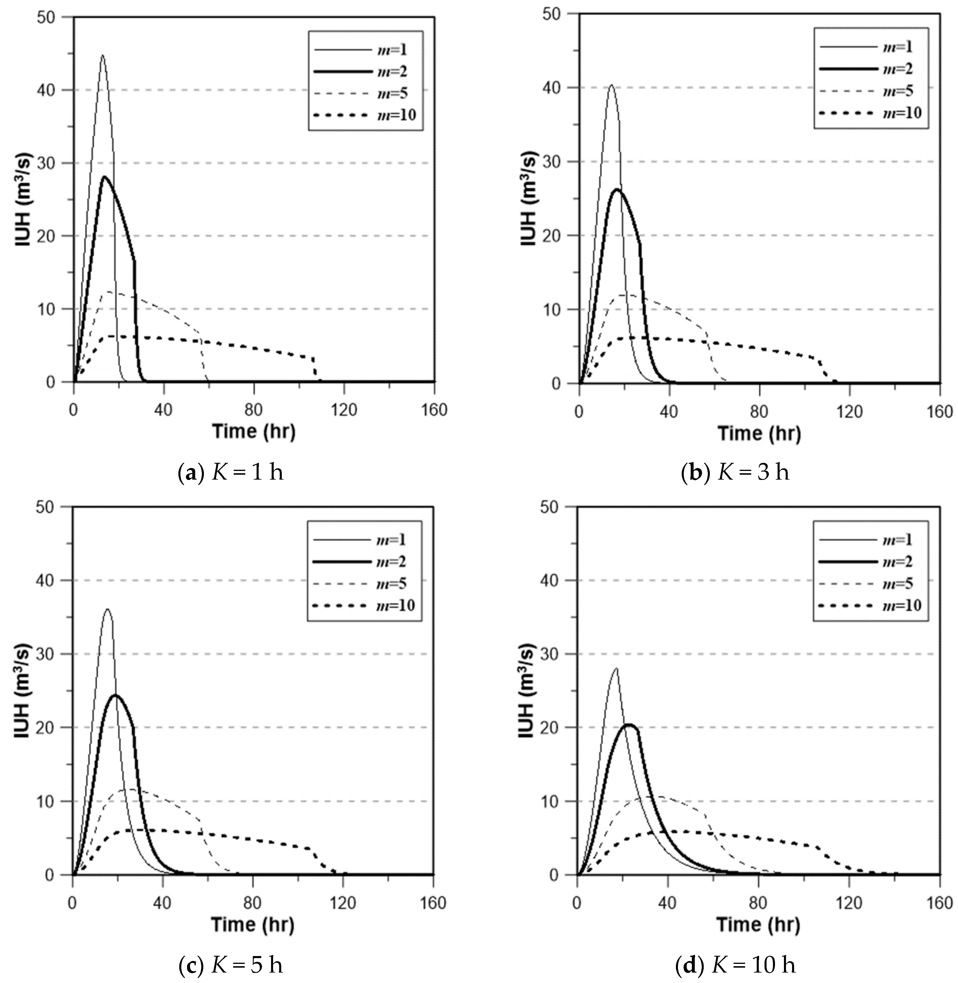
As an example, this study considered an elliptical basin with an area of 188.50 km2. The transverse and conjugate diameters were 20 and 12 km, respectively. Additionally, for the derivation of the Clark IUH, the channel velocity was assumed to be 1 km/h (approximately 0.28 m/s). The hillslope velocity was then determined by assigning four different m values (i.e., m = 1, 2, 5, and 10). This study also considered four different storage coefficients (i.e., 1, 3, 5, and 10 h) in order to find their effect on the shape of the Clark IUH. Figure 2 compares the derived Clark IUHs.
Figure 2 shows that both the effect of m and the storage coefficient on the Clark IUH are very clear. The effect of m can be easily found in Figure 2a, where a very small storage coefficient was applied. For a small m, that is, when the hillslope velocity is very high, the runoff peak flow is very high. As m becomes higher, the runoff peak flow becomes much lower. However, in all cases of m, the peak time seems to remain almost unchanged. In fact, this result is easily understandable, as in Figure 2a, the storage effect is almost negligible.
On the other hand, in Figure 2b–d, the storage effect becomes very significant in other cases, where a very different peak time is derived. As a larger storage coefficient is applied, a much smoother Clark IUH with lower runoff peak and longer peak time is derived. The effect of the storage coefficient on the falling limb of the Clark IUH is also noticeable. Recall that the concentration time remains unchanged, regardless of the high storage coefficient. The storage coefficient also controls the peak time but not the concentration time. The concentration time is dependent upon the ratio between the channel and hillslope velocities, or the value of m in this study. For reference, the concentration time of this basin was estimated for each m value in Table 1. In fact, the concentration time could be estimated simply by dividing by the channel velocity. Additionally, Table 1 shows the peak flow and peak time that were derived for comparison with the concentration time.
3. Study Basin and Rainfall Events
3.1. Study Basin
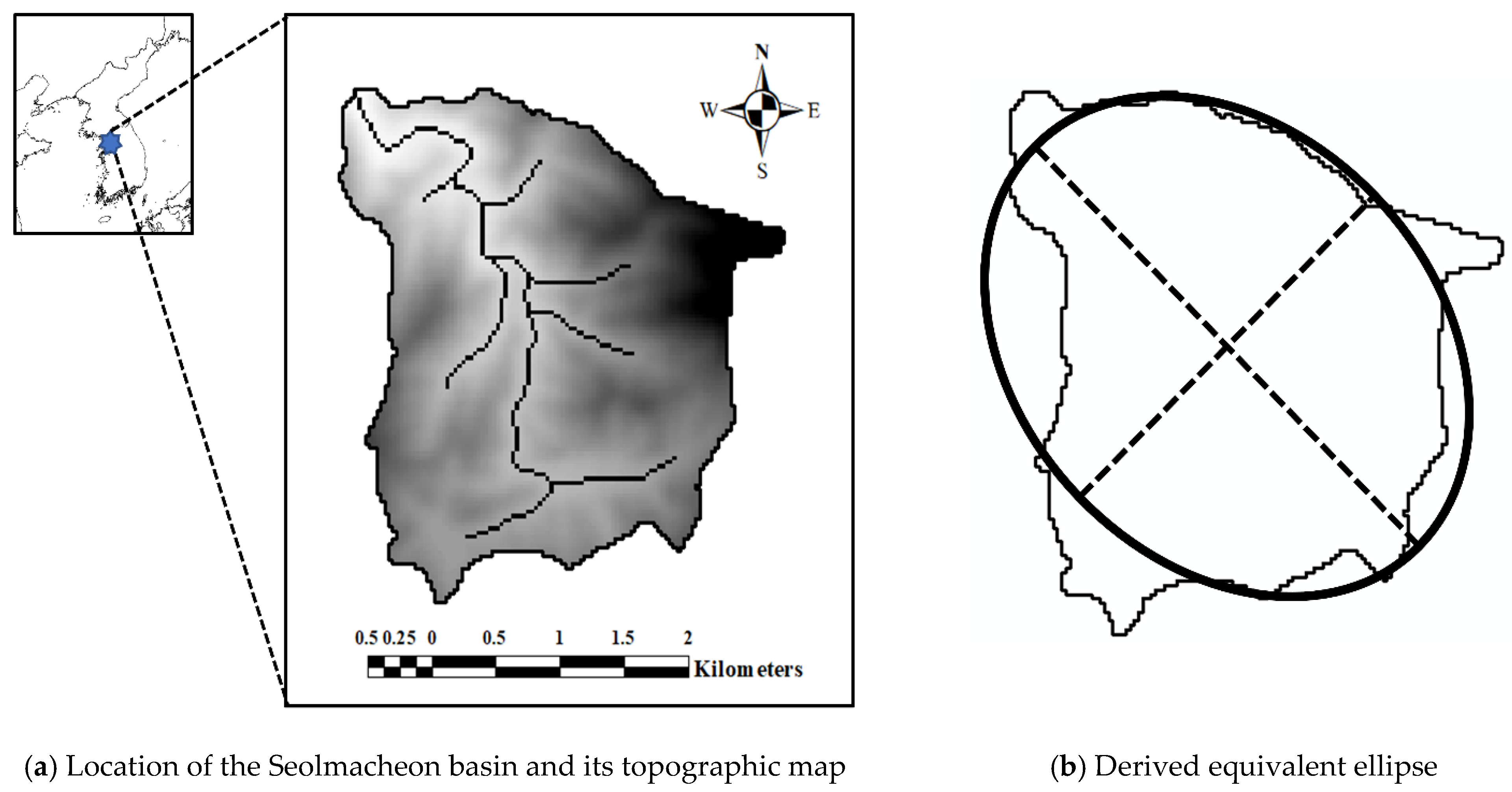
This study analyzed the rainfall–runoff relationship of the Seolmacheon basin in Korea (Figure 3). The Seolmacheon basin is a mountainous basin covered by various coniferous and deciduous trees. The basin area is about 8.5 km2, and the length of the main channel is about 8.8 km, with a slope of 3.3%. The soil is mostly sandy loam, and its depth is known to be very shallow, i.e., less than 1 m in most areas [70]. The annual precipitation is about 1210 mm, and the mean temperature is around 11.5 °C. Most of the rainfall (about 70%) occurs during the summer season, from June to September [71].
The Seolmacheon basin is an experimental basin managed by the Korea Institute of Civil Engineering and Building Technology (KICT). This is the reason why this small basin has six rain gauges within it, measuring the rain rate every 10 min. The water stage is also measured every 10 min at a bridge at the exit of the basin. The rating curve is updated every year, and by applying the corresponding rating curve, the water depth data can be converted into the runoff data. A flux tower at the center of the basin measures various parameters to estimate the evaporation and transpiration. Several time-domain reflectometry (TDR) sensors are also managed to measure the variation of soil moisture.
The method by Moussa (2003) [45] was applied to derive the equivalent ellipse representing the study basin. The method is based on the following four assumptions. First, the center of the ellipse coincides with the center of the given basin. Second, the major axis of the ellipse coincides with the major inertia axis of the basin. Third, the area of the ellipse should be the same as that of the basin. Fourth, the ratios between the maximum and minimum inertia moments in both the ellipse and the basin should be the same. Figure 3b shows the equivalent ellipse that was derived for the Seolmacheon basin. In this figure, the derived equivalent ellipse is overlapped by coinciding both the center and the major axes of the basin. As the geometrical shapes of the basin and derived ellipse match well, the derived equivalent ellipse is assumed to adequately represent the basin. The determined transverse and conjugate diameters of the ellipse are 3.6 and 3.0 km, respectively.
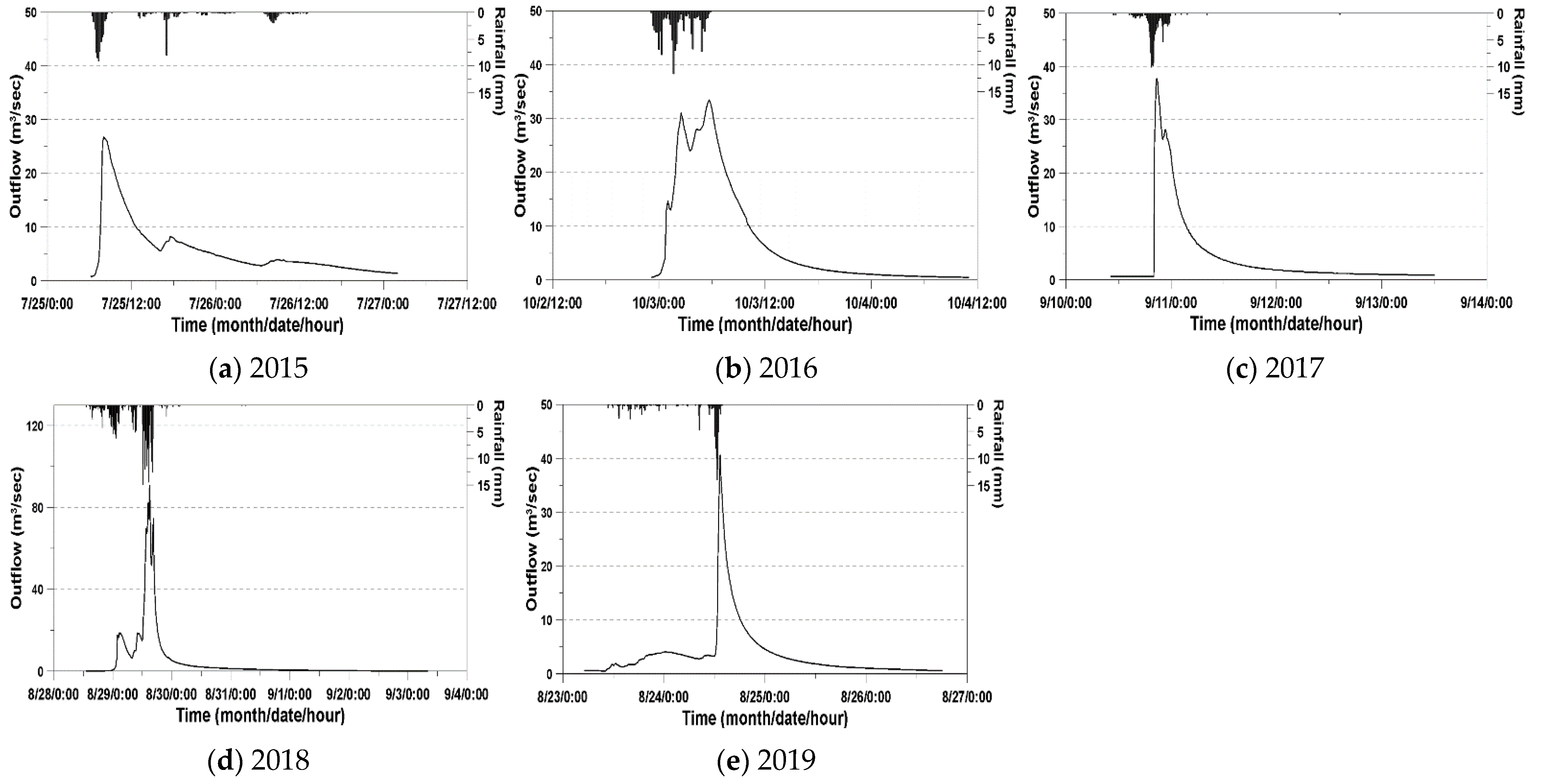
3.2. Rainfall Events
A total of five rainfall events were selected for analysis in this study. These rainfall events were the largest in each year from 2015 to 2019. Four events occurred during the wet summer season from July to September, and the fifth was in October during Typhoon Chaba. The biggest rainfall event among the five occurred on 28 August 2018, and lasted 39 h. The total rainfall amount was 315.1 mm, with a highest rainfall intensity of 53.0 mm/h being recorded on 29 August at 14:40. The smallest event occurred on 25 July 2015, and lasted 30 h. The total rainfall amount was 99.6 mm, and its highest intensity was 42.5 mm/h, recorded on 25 July at 07:30.
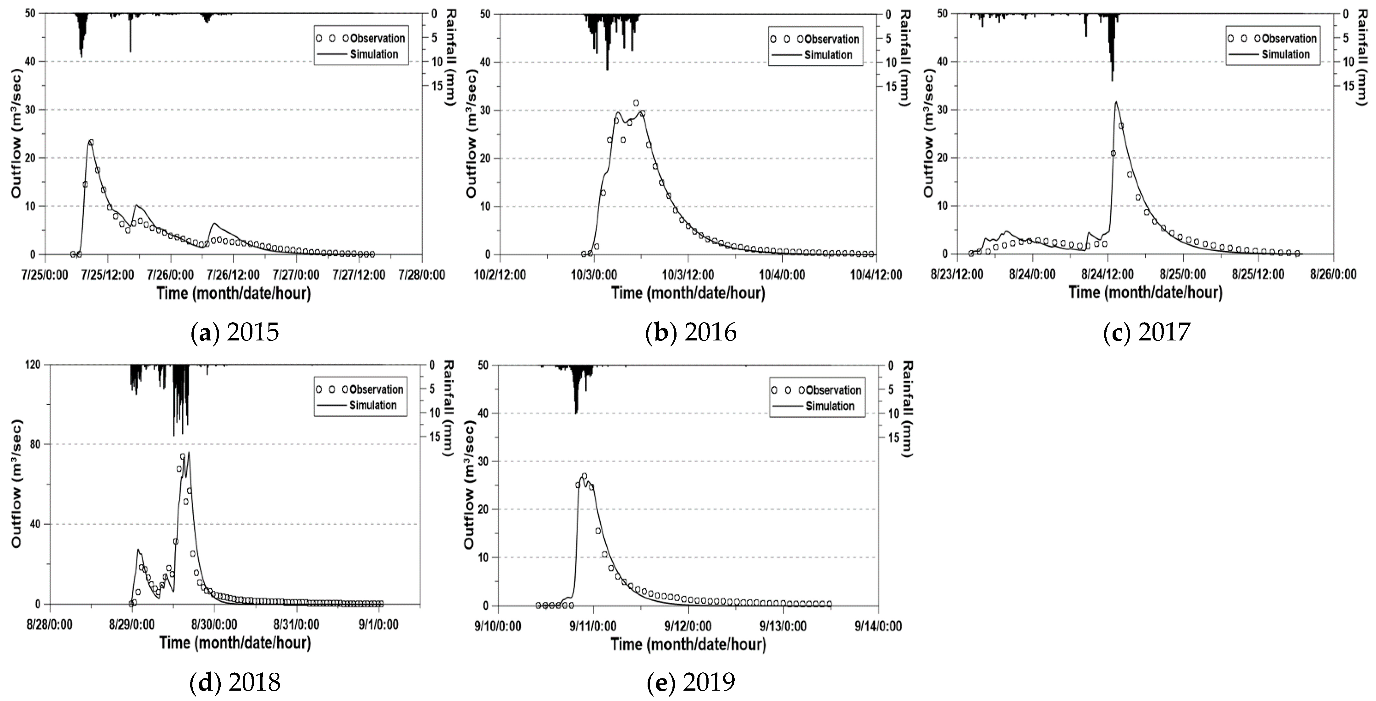
The areal-average rainfall data was estimated by applying the Thiessen polygon method, and the runoff data was derived by applying the rating curve to the water stage data measured at the exit of the basin. The cross-sectional mean channel velocity was also estimated using the runoff data and the cross-sectional area corresponding to the water stage. For example, for the rainfall event in 2018, the peak channel velocity was estimated to be 3.06 m/s, but for other rainfall events, the peak channel velocities were all less than 2.5 m/s. Figure 4 shows the rainfall–runoff data used in this study. Also, Table 2 summarizes the detailed information about these rainfall events.
4. Results and Discussions
4.1. Clark IUH for Uniform Velocity Case (Baseline Case)
The analytically-derived Clark IUH in Section 2 is a function of the channel velocity, hillslope velocity, and storage coefficient. In this section, however, both the channel and hillslope velocity were assumed to be identical (in this study, this case was used as the baseline). This assumption is general for most IUH models [9,10,11,63]. Also, the peak flow velocity measured at the exit of the basin was used for both the channel and hillslope velocities. The use of the peak flow velocity was based on Rodriguez-Iturbe and Valdes (1979) [63]. Additionally, as the storage coefficient variedso much depending on the rainfall event, this study estimated the storage coefficient separately for each rainfall event. In this step, the method proposed by Yoo et al. (2014) was used [37]. Yoo et al. (2014) showed that the concentration time and the storage coefficient of the Clark IUH could be estimated by analyzing the observed rainfall–runoff data [37]. The derived storage coefficient for each rainfall event was then applied to the analytically-derived Clark IUH. Finally the runoff hydrograph could be simulated by applying this analytically-derived Clark IUH.
To estimate the concentration time and storage coefficient of the Clark IUH using the method by Yoo et al. (2014) [37], the effective rainfall and the direct runoff data had to first be derived. In this study, the straight-line method was used to separate the direct runoff from the total runoff, while the Φ-index method was used to estimate the effective rainfall [33]. However, in this study, as the main channel of the Seolmacheon basin was mostly dry, the separation of the direct runoff was not necessary. Using the derived effective rainfall and direct runoff data, the concentration time and the storage coefficient were estimated using the method of Yoo et al. (2014) for each rainfall event [37].
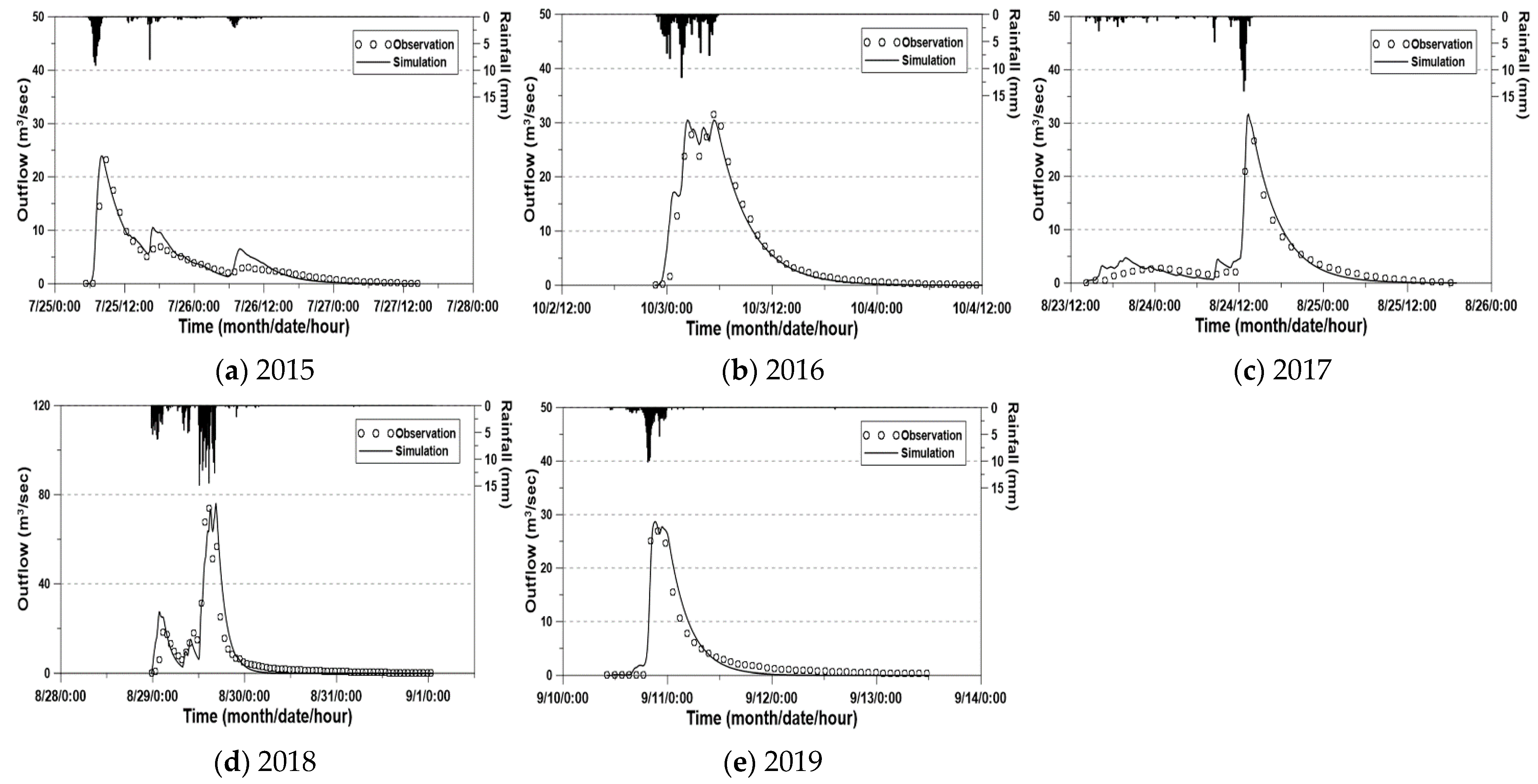
Figure 5 compares these two hydrographs derived for all five rainfall events. As shown in this figure, the two observed and simulated runoff hydrographs were very similar to each other. Even though the difference was not great, in the rainfall events observed in 2015 and 2016, the runoff hydrographs based on the analytically-derived Clark IUH showed a slightly higher peak flow but shorter peak time. On the other hand, the opposite result was derived in the rainfall event observed in 2018, that is, the runoff hydrograph based on the analytically-derived Clark IUH showed a slightly smaller peak flow but a slightly longer peak time. Finally, in the other two rainfall events observed in 2017 and 2019, no obvious difference in peak flow and peak time could be found.
4.2. Clark IUH for Different Velocity Case (Consideration of the Hillslope Velocity)
In this section, the hillslope velocity was assumed to be not necessarily equal to the channel velocity. The hillslope velocity was determined by comparing the observed and simulated runoff hydrographs using the minimum root mean square error. That is, under the condition that the channel velocity is given by the peak flow velocity measured at the exit of the basin, the hillslope velocity was determined by comparing the observed runoff hydrograph and the simulated one. This procedure was repeated for all five rainfall events, and thus, five different hillslope velocities were estimated. In this study, the ratio between the channel velocity and the hillslope velocity was assumed to be within the range of 1 to 20. Based on D’Odorico and Rigon (2003), the general ratio ranges from 5 to 20 [1].
Table 3 summarizes the estimation result of the hillslope velocity. Obviously, the hillslope velocity varied considerably depending on the rainfall event. The ratio between the channel velocity and the hillslope velocity was estimated to be minimum 1 and maximum 6, which is within the range from 1 to 20 assumed in this study based on D’Odorico and Rigon (2003) [1]. The ratio for the rainfall events observed in 2017 and 2018 was estimated to be 1, while for the rainfall event in 2019, it was 1.7. On the other hand, for the rainfall events in 2015 and 2016, the ratio was 4.4 and 6.0, respectively. In the case where the difference between the two runoff hydrographs compared in the previous section was large, the ratio was estimated to be quite high.
Figure 6 shows how the simulated runoff hydrographs became similar to the observed one as the hillslope velocity was considered. The difference between the observed and simulated runoff hydrographs almost disappeared. The effect of the hillslope velocity was clearly dominant with regard to the peak time and peak flow, as in the rainfall event observed in 2016; however, its effect could also be found in the sudden drop off after the peak time, as in the rainfall event observed in 2019. The simulated runoff hydrographs considering the proper hillslope velocity showed a one-step better fit in the falling limb.
The qualitative evaluation result in the previous paragraph was also confirmed by the quantitative evaluation measures like the root mean square error (RMSE) and the coefficient of determination (R2). Table 4 summarizes the comparison result between the uniform velocity case (Section 4.1) and the different velocity case (Section 4.2). As shown in this table, the different velocity case of considering both the channel and hillslope velocities provides a better fit than the uniform velocity case. Especially when m was very high (i.e., when the hillslope velocity is much lower than the channel velocity), the different velocity case showed much better simulation result.
Another interesting point can be seen in the comparison of concentration times. Table 5 compares the concentration times derived for three different cases; the first is based on the observed rainfall-runoff analysis using the method by Yoo et al. (2014) [37], the second is the uniform velocity case, and the third is the different velocity case for considering both the channel and hillslope velocity. As a final outcome, the authors notices that the concentration times estimated by considering both the channel and hillslope velocities became very similar to those estimated by analyzing the observed runoff hydrograph. That is, when considering the uniform flow velocity over the entire basin including the channel and hillslope, the estimated concentration time was vastly different from reality. This result is also in line with the definition of the concentration time. The concentration time simply represents the time required for the raindrop located at the farthest point of a given basin to reach the exit of the basin. This should be estimated by considering different channel and hillslope velocities. This result shows that the hillslope velocity could play a key role in estimating the concentration time. However, it should also be mentioned that the role of the hillslope velocity is highly dependent on the rainfall event itself. In some rainfall events, the effect of the hillslope velocity is very high, but in other cases, it is not. At this time, what makes the difference is not clear.
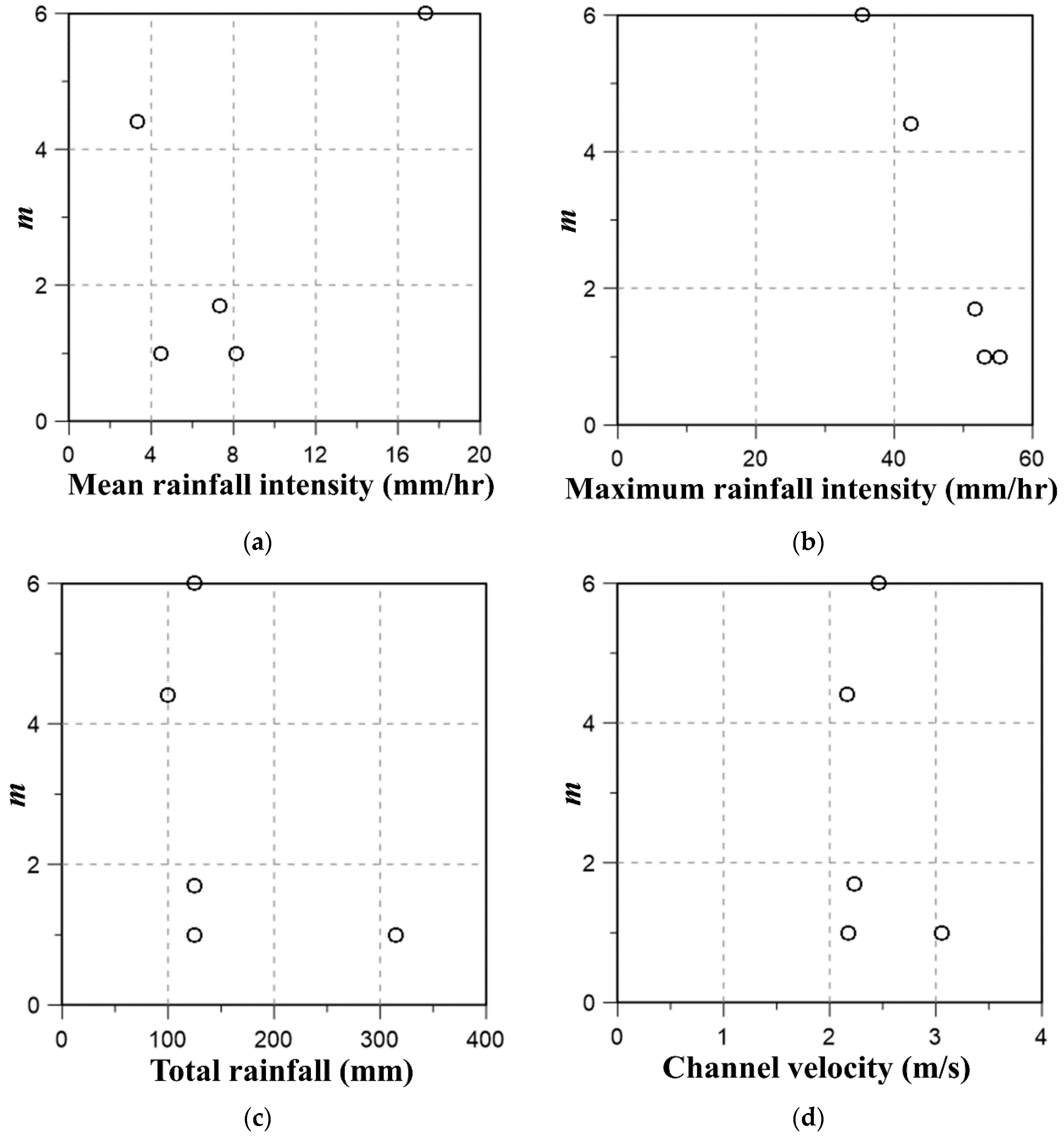
Additionally, to look for the key factor controlling the ratio between the channel and the hillslope velocities, several scatter plots were made, including those shown in Figure 7. Mean rainfall intensity, maximum rainfall intensity, total rainfall, and the channel velocity were considered as independent factors. In the cases with the mean rainfall intensity, total rainfall, and channel velocity, no obvious dependency could be found. However, in the case considering the maximum rainfall intensity, a clear inverse proportionality could be observed, as in Figure 7b. The correlation coefficient between the two was also found to be higher than 0.9. Based on this finding, it could be concluded that the maximum rainfall intensity controls the representative flow velocity in the hillslope region, which, in turn, controls the shape of the runoff hydrograph. As the maximum rainfall intensity increases, the hillslope velocity approaches the channel velocity. Except for the rainfall event which occurred in 2018, the channel velocities of the rainfall events were all estimated similarly, and thus, it was found that the concentration time of the Clark IUH was controlled by the hillslope velocity. This is the reason why the Clark IUH determined by considering both the channel and hillslope velocities provided the most similar concentration times to those based on the analysis of the observed rainfall–runoff data.
4.3. Discussions
The findings in this study show that hillslope velocity can be a key factor in determining the shape of the basin IUH. The role of the hillslope velocity was also confirmed in the application of the Clark IUH to the Seolmacheon basin, Korea. That is, in the case of considering both the channel velocity and hillslope velocity, better results of runoff simulation could be confirmed qualitatively and quantitatively. This result is in line with various previous studies [1,2,3].
This study, however, is different from other studies in some respects. First of all, the model considered in this study is a simple synthetic unit hydrograph. Most previous studies were based on the distributed model [23,24,25,26,27]. Even though the hillslope velocity was considered, its overall effect on the runoff at the exit of the basin could not be quantified easily in the distributed models. This study thus has the technical ability to consider the overall effect of hillslope velocity on the shape of the basin response function. It was very easy to compare the change of the shape of Clark IUH before and after consideration of hillslope velocity, as shown in Figure 2.
The use of a synthetic unit hydrograph in this study has some advantages. One important advantage is that the overall effect of the hillslope velocity could easily be distinguished. Analytical derivation of the time–area curve and the Clark IUH is another important advantage of this study, as the effect of hillslope velocity can easily be tracked. Under the condition that the channel velocity remains unchanged, the hillslope velocity was found to control the runoff peak flow, but not the peak time. The hillslope velocity also controlled the concentration time. Also, the analytical time–area curve in this study can be differentiated from the typical methods like the isosceles triangle and nonlinear curve, as the time–area curve in this study can be derived by considering the translational effect in the hillslope area [34,35,72,73,74].
However, these advantages also bring about disadvantages. First, it is not clear how to determine the representative value of the hillslope velocity. This value was estimated in this study for each rainfall event by minimizing the difference between simulated and observed runoff hydrographs. Thus, the meaning of this value of hillslope velocity became ambiguous. It was shown by the sensitivity analysis that the representative hillslope velocity was related to the rainfall intensity. These fundamental limitations must be overcome with more applications to basins, from small to large. Also, more measurements of the velocity on various hillslopes could be helpful in overcoming the limitations of this study.
It was assumed that the perpendicular flow direction from hillslope to channel adopted in this study is another limitation. As a future study, a more general case of considering the oblique flow direction should be investigated. As the overland flow length is elongated by considering the oblique flow direction, the role of hillslope can be differently quantified. Finally, it should also be mentioned that this is just one application example. The findings in this study may not be generalized quantitatively.
5. Conclusions
In this study, the effect of the hillslope velocity was investigated using the Clark IUH. First, the time–area curve of an ellipse was analytically derived by considering flow velocities within the channel and hillslope. Also, by applying the derived time–area curve as an input to the linear reservoir, the Clark IUH was analytically derived. The derived Clark IUH was then evaluated by considering various sets of channel and hillslope velocities. Finally, the derived Clark IUH was evaluated by applying it to the Seolmacheon basin, a small mountainous basin in Korea. The results of this study may be summarized as follows:
First, the time–area curve of an ellipse was derived analytically, which was then used to find the effect of the hillslope velocity on the shape of the time–area curve. The Clark IUH was also derived analytically by solving the continuity equation, along with the input of the derived time–area curve to the linear reservoir model. The derived Clark IUH was found to be very sensitive to both the hillslope velocity and the storage coefficient. In particular, it was possible to distinguish the effect of the hillslope velocity from that of the storage coefficient. The hillslope velocity was found to control the runoff peak flow and the concentration time. On the other hand, the storage coefficient controlled the peak time, peak flow, and the shape of the falling limb of the Clark IUH.
Second, similar results were derived in the application of the Clark IUH to the Seolmacheon basin in Korea. In particular, it was confirmed that the role of hillslope velocity is a key factor in determining the concentration time of the given basin. When considering both the channel and hillslope velocities, the concentration time was found to be most similar to that derived by analyzing the observed rainfall–runoff events. However, it was also found that the hillslope velocity varied considerably, depending on the rainfall event.
Finally, the maximum rainfall intensity was found to be the most important factor to control the hillslope velocity. In fact, this finding is in line with previous studies, like those of Rodriguez-Iturbe et al. (1979), Bhaskar et al. (1997), and Sahoo et al. (2006) [11,75,76]. In those studies, the representative channel velocity was determined as the maximum one for the given rainfall event. Similarly, the representative channel velocity should be determined to be the maximum one by considering the maximum rainfall intensity. In fact, this result can also be easily understood as both the runoff peak time and the concentration time being controlled by the velocities in both the channel and hillslope.
Author Contributions
Data curation, C.J. and W.N.; Formal analysis, H.P.D. and W.N.; Methodology, C.Y.; Supervision, C.Y.; Visualization, H.P.D. and W.N.; Writing—original draft, C.Y.; Writing—review & editing, C.J. and W.N. All authors have read and agreed to the published version of the manuscript.
Funding
This work was supported by the National Research Foundation of Korea (NRF) grant funded by the Korea government (MSIT) (No. 2020R1A2C2008714), and the National Research Foundation of Korea (NRF) grant funded by the Korea government (MSIT) (No. NRF-2021R1A5A1032433).
Institutional Review Board Statement
Not applicable.
Informed Consent Statement
Not applicable.
Data Availability Statement
Not applicable.
Conflicts of Interest
The authors declare no conflict of interest.
References
- D’Odorico, P.; Rigon, R. Hillslope and channel contributions to the hydrologic response. Water Resour. Res. 2003, 39, WR001708. [Google Scholar] [CrossRef]
- Van der Tak, L.D.; Bras, R.L. Incorporating hillslope effects into the geomorphological instantaneous unit hydrograph. Water Resour. Res. 1990, 26, 2393–2400. [Google Scholar] [CrossRef]
- Robinson, J.S.; Sivapalan, M.; Snell, J.D. On the relative roles of hillslope processes, channel routing, and network morphology in the hydrologic response of natural catchments. Water Resour. Res. 1995, 31, 3089–3101. [Google Scholar] [CrossRef]
- Rinaldo, A.; Vogel, G.K.; Rigon, R.; Rodriguez-Iturbe, I. Can one gauge the shape of a basin? Water Resour. Res. 1995, 31, 1119–1127. [Google Scholar] [CrossRef]
- Snell, J.D.; Sivapalan, M. On geomorphological dispersion in natural catchments and the geomorphological unit hydrograph. Water Resour. Res. 1994, 30, 2311–2323. [Google Scholar] [CrossRef]
- Maidment, D.R.; Olivera, F.; Calver, A.; Eatherall, A.; Fraczek, W. Unit hydrograph derived from a spatially distributed velocity field. Hydrol. Process. 1996, 10, 831–844. [Google Scholar] [CrossRef]
- Muzik, I. Flood modelling with GIS-derived distributed unit hydrographs. Hydrol. Process. 1996, 10, 1401–1409. [Google Scholar] [CrossRef]
- Rodriguez, F.; Andrieu, H.; Creutin, J.D. Surface runoff in urban catchments: Morphological identification of unit hydrographs from urban databanks. J. Hydrol. 2003, 283, 146–168. [Google Scholar] [CrossRef]
- Pilgrim, D.H. Travel times and nonlinearity of flood runoff from tracer measurements on a small watershed. Water Resour. Res. 1976, 12, 487–496. [Google Scholar] [CrossRef]
- Grimaldi, S.; Petroselli, A.; Alonso, G.; Nardi, F. Flow time estimation with spatially variable hillslope velocity in ungauged basins. Adv. Water Resour. 2010, 33, 1216–1223. [Google Scholar] [CrossRef]
- Sahoo, B.; Chatterjee, C.; Raghuwanshi, N.S.; Singh, R.; Kumar, R. Flood estimation by GIUH-based Clark and Nash models. J. Hydrol. Eng. 2006, 11, 515–525. [Google Scholar] [CrossRef]
- Rodríguez-Iturbe, I.; González-Sanabria, M.; Bras, R.L. A geomorphoclimatic theory of the instantaneous unit hydrograph. Water Resour. Res. 1982, 18, 877–886. [Google Scholar] [CrossRef]
- Rinaldo, A.; Marani, A.; Rigon, R. Geomorphological dispersion. Water Resour. Res. 1991, 27, 513–525. [Google Scholar] [CrossRef]
- Kumar, R.; Chatterjee, C.; Singh, R.D.; Lohani, A.K.; Kumar, S. Runoff estimation for an ungauged catchment using geomorphological instantaneous unit hydrograph (GIUH) models. Hydrol. Process. 2007, 21, 1829–1840. [Google Scholar] [CrossRef]
- Clark, C.O. Storage and the unit hydrograph. Trans. Am. Soc. Civil Eng. 1945, 110, 1419–1446. [Google Scholar] [CrossRef]
- Gyasi-Agyei, Y.; De Troch, F.P.; Troch, P.A. A dynamic hillslope response model in a geomorphology based rainfall-runoff model. J. Hydrol. 1996, 178, 1–18. [Google Scholar] [CrossRef]
- Yang, D.; Herath, S.; Musiake, K. A hillslope-based hydrological model using catchment area and width functions. Hydrol. Sci. J. 2002, 47, 49–65. [Google Scholar] [CrossRef]
- Di Lazzaro, M. Regional analysis of storm hydrographs in the rescaled width function framework. J. Hydrol. 2009, 373, 352–365. [Google Scholar] [CrossRef]
- Grimaldi, S.; Petroselli, A.; Nardi, F. A parsimonious geomorphological unit hydrograph for rainfall–runoff modelling in small ungauged basins. Hydrol. Sci. J. 2012, 57, 73–83. [Google Scholar] [CrossRef]
- Zhang, H.L.; Wang, Y.J.; Wang, Y.Q.; Li, D.X.; Wang, X.K. The effect of watershed scale on HEC-HMS calibrated parameters: A case study in the Clear Creek watershed in Iowa, US. Hydrol. Earth Syst. Sci. 2013, 17, 2735–2745. [Google Scholar] [CrossRef] [Green Version]
- Arnold, J.G.; Allen, P.M.; Volk, M.; Williams, J.R.; Bosch, D.D. Assessment of different representations of spatial variability on SWAT model performance. Trans. ASABE 2010, 53, 1433–1443. [Google Scholar] [CrossRef]
- Rathjens, H.; Oppelt, N.; Bosch, D.D.; Arnold, J.G.; Volk, M. Development of a grid-based version of the SWAT landscape model. Hydrol. Process. 2015, 29, 900–914. [Google Scholar] [CrossRef]
- Hoang, L.; Schneiderman, E.M.; Moore, K.E.; Mukundan, R.; Owens, E.M.; Steenhuis, T.S. Predicting saturation-excess runoff distribution with a lumped hillslope model: SWAT-HS. Hydrol. Process. 2017, 31, 2226–2243. [Google Scholar] [CrossRef]
- Bouraoui, F.; Dillaha, T.A. ANSWERS-2000: Runoff and sediment transport model. J. Environ. Eng. 1996, 122, 493–502. [Google Scholar] [CrossRef]
- Downer, C.W.; Ogden, F.L. Gridded Surface Subsurface Hydrological Analysis (GSSHA) User’s Manual; Version 1.43 for Watershed Modeling System 6.1; Engineer Research and Development Center, U.S. Army Corps of Engineers: Washington, DC, USA, 2006. [Google Scholar]
- Zhang, Y.; Shuster, W. The Comparative Accuracy of Two Hydrologic Models in Simulating Warm-Season Runoff for Two Small, Hillslope Catchments. J. Am. Water Resour. Assoc. 2014, 50, 434–447. [Google Scholar] [CrossRef]
- Vázquez, R.F.; Feyen, J. Assessment of the effects of DEM gridding on the predictions of basin runoff using MIKE SHE and a modelling resolution of 600 m. J. Hydrol. 2007, 334, 73–87. [Google Scholar] [CrossRef]
- Noh, S.J.; An, H.; Kim, S.; Kim, H. Simulation of soil moisture on a hillslope using multiple hydrologic models in comparison to field measurements. J. Hydrol. 2015, 523, 342–355. [Google Scholar] [CrossRef]
- Loritz, R.; Hassler, S.K.; Jackisch, C.; Allroggen, N.; Schaik, L.V.; Wienhöfer, J.; Zehe, E. Picturing and modeling catchments by representative hillslopes. Hydrol. Earth Syst. Sci. 2017, 21, 1225–1249. [Google Scholar] [CrossRef] [Green Version]
- Heerdegen, R.G.; Reich, B.M. Unit hydrographs for catchments of different sizes and dissimilar regions. J. Hydrol. 1974, 22, 143–153. [Google Scholar] [CrossRef]
- Jakeman, A.J.; Littlewood, I.G.; Whitehead, P.G. Computation of the instantaneous unit hydrograph and identifiable component flows with application to two small upland catchments. J. Hydrol. 1990, 117, 275–300. [Google Scholar] [CrossRef]
- Cleveland, T.G.; He, X.; Asquith, W.H.; Fang, X.; Thompson, D.B. Instantaneous unit hydrograph evaluation for rainfall-runoff modeling of small watersheds in north and south central Texas. J. Irrig. Drain. Eng. 2006, 132, 479–485. [Google Scholar] [CrossRef]
- Chow, V.T. Applied Hydrology; Tata McGraw-Hill Education: New York, NY, USA, 2010. [Google Scholar]
- Ahmad, M.M.; Ghumman, A.R.; Ahmad, S. Estimation of Clark’s instantaneous unit hydrograph parameters and development of direct surface runoff hydrograph. Water Resour. Manag. 2009, 23, 2417–2435. [Google Scholar] [CrossRef]
- Seong, K.W.; Lee, Y.H. A practical estimation of Clark IUH parameters using root selection and linear programming. Hydrol. Process. 2011, 25, 3676–3687. [Google Scholar] [CrossRef]
- Osman, S.; Abustan, I. Estimating the Clark Instantaneous Unit Hydrograph parameters for selected gauged catchments in the west Coast of Peninsular Malaysia. ASEAN Eng. J. 2011, 1, 126–141. [Google Scholar]
- Yoo, C.; Lee, J.; Park, C.; Jun, C. Method for estimating concentration time and storage coefficient of the Clark model using rainfall-runoff measurements. J. Hydrol. Eng. 2014, 19, 626–634. [Google Scholar] [CrossRef]
- Kar, K.K.; Yang, S.K.; Lee, J.H. Assessing unit hydrograph parameters and peak runoff responses from storm rainfall events: A case study in Hancheon Basin of Jeju Island. J. Environ. Sci. Int. 2015, 24, 437–447. [Google Scholar] [CrossRef] [Green Version]
- Hemmati, M.; Shahnazi, M.; Ahmadi, H.; Salarjazi, M. Flood Peak Flow Simulation and Determination of Flood Source Area in the QARANQU Watershed Using Hydrological Mod-Clark Model and GIS. Irrig. Water Eng. 2017, 7, 65–80. [Google Scholar]
- Cho, Y.; Engel, B.A.; Merwade, V.M. A spatially distributed Clark’s unit hydrograph based hybrid hydrologic model (Distributed-Clark). Hydrol. Sci. J. 2018, 63, 1519–1539. [Google Scholar] [CrossRef]
- Moradi, H.R.; Asadi, H.; Sadeghi, S.H.; Telvari, A. Evaluation of Time-Area Accuracy in Developing IUH. J. Range Watershed Manag. 2015, 68, 647–656. [Google Scholar]
- Sabzevari, T. Runoff prediction in ungauged catchments using the gamma dimensionless time-area method. Arab. J. Geosci. 2017, 10, 131. [Google Scholar] [CrossRef]
- Fariborzi, H.; Sabzevari, T.; Noroozpour, S.; Mohammadpour, R. Prediction of the subsurface flow of hillslopes using a subsurface time-area model. Hydrogeol. J. 2019, 27, 1401–1417. [Google Scholar] [CrossRef]
- Jun, C.; Yoo, C. Relative roles of time-area curve and storage coefficient on the shape of Clark’s instantaneous unit hydrograph: An analytical approach. J. Hydrol. Eng. 2021, 26, 06021001. [Google Scholar] [CrossRef]
- Moussa, R. On morphometric properties of basins, scale effects and hydrological response. Hydrol. Process. 2003, 17, 33–58. [Google Scholar] [CrossRef]
- USACE (United States Army Corps of Engineers). Hydrologic Modeling System HEC-HMS: User’s Manual; US Army Corps of Engineers: Washington, DC, USA, 2016. [Google Scholar]
- Langbein, W.B. Topographic Characteristics of Drainage Basins; U.S. Geological Survey: Reston, VA, USA, 1947. [Google Scholar]
- Taylor, A.B.; Schwarz, H.E. Unit hydrograph lag and peak flow related to basin characteristics. Eos Trans. Am. Geophys. Union. 1952, 33, 235–246. [Google Scholar] [CrossRef]
- Wu, I.P. Design hydrographs for small watershed in Indiana. J. Hydraul. Division. 1963, 89, 36–65. [Google Scholar] [CrossRef]
- Kim, J.C.; Jung, K.S.; Kim, J.H. The correlation analysis between new catchment shape descriptor and the lag time of Nash model. J. Korea Water Resour. Assoc. 2004, 37, 1065–1074. [Google Scholar] [CrossRef]
- McCuen, R.H. Hydrologic Analysis and Design, 3rd ed.; Prentice Hall: New Jersey, NJ, USA, 2005. [Google Scholar]
- Huff, F.A. Time distribution of rainfall in heavy storms. Water Resour. Res. 1967, 3, 1007–1019. [Google Scholar] [CrossRef]
- Hansen, E.M.; Schreiner, L.C.; Miller, J.F. Application of Probable Maximum Precipitation Estimates—United States East of the 105th Meridian, Hydrometeorological Report No. 52; National Weather Service: Washington, DC, USA, 1982. [Google Scholar]
- Suyanto, A.; O’Connell, P.E.; Metcalfe, A.V. The influence of storm characteristics and catchment conditions on extreme flood response: A case study based on the Brue river basin. U.K. Surv. Geophys. 1995, 16, 201–225. [Google Scholar] [CrossRef]
- USACE (United States Army Corps of Engineers). Hydrologic Modeling System HEC-HMS Technical Reference Manual; Hydrologic Engineering Center: Davis, CA, USA, 2000. [Google Scholar]
- Singh, S.K. Clark’s and Espey’s unit hydrographs vs. the gamma unit hydrograph. Hydrol. Sci. J. 2005, 50, 1053–1067. [Google Scholar]
- Quinn, P.F.B.J.; Beven, K.; Chevallier, P.; Planchon, O. The prediction of hillslope flow paths for distributed hydrological modelling using digital terrain models. Hydrol. Process. 1991, 5, 59–79. [Google Scholar] [CrossRef]
- Onda, Y.; Tsujimura, M.; Tabuchi, H. The role of subsurface water flow paths on hillslope hydrological processes, landslides and landform development in steep mountains of Japan. Hydrol. Process. 2004, 18, 637–650. [Google Scholar] [CrossRef]
- Tarolli, P.; Dalla Fontana, G. Hillslope-to-valley transition morphology: New opportunities from high resolution DTMs. Geomorphology 2009, 113, 47–56. [Google Scholar] [CrossRef]
- Sabzevari, T.; Noroozpour, S. Effects of hillslope geometry on surface and subsurface flows. Hydrogeol. J. 2014, 22, 1593–1604. [Google Scholar] [CrossRef]
- Scaini, A.; Hissler, C.; Fenicia, F.; Juilleret, J.; Iffly, J.F.; Pfister, L.; Beven, K. Hillslope response to sprinkling and natural rainfall using velocity and celerity estimates in a slate-bedrock catchment. J. Hydrol. 2018, 558, 366–379. [Google Scholar] [CrossRef]
- Wacha, K.M.; Papanicolaou, A.N.; Giannopoulos, C.P.; Abban, B.K.; Wilson, C.G.; Zhou, S.; Hatfield, J.L.; Filley, T.R.; Hou, T. The role of hydraulic connectivity and management on soil aggregate size and stability in the Clear Creek Watershed, Iowa. Geosciences 2018, 8, 470. [Google Scholar] [CrossRef] [Green Version]
- Rodriguez-Iturbe, I.; Valdes, J.B. The geomorphologic structure of hydrologic response. Water Resour. Res. 1979, 15, 1409–1420. [Google Scholar] [CrossRef] [Green Version]
- Gupta, V.K.; Waymire, E.C.; Wang, C.T. A representation of an instantaneous unit hydrograph from geomorphology. Water Resour. Res. 1980, 16, 855–862. [Google Scholar] [CrossRef]
- Ascough, J.C., II; Baffaut, C.; Nearing, M.A.; Liu, B.Y. The WEPP watershed model: I. Hydrology and erosion. Trans. ASAE 1997, 40, 921–933. [Google Scholar] [CrossRef]
- Broda, S.; Larocque, M.; Paniconi, C. Simulation of distributed base flow contributions to streamflow using a hillslope-based catchment model coupled to a regional-scale groundwater model. J. Hydrol. Eng. 2014, 19, 907–917. [Google Scholar] [CrossRef]
- Hallema, D.W.; Moussa, R. A model for distributed GIUH-based flow routing on natural and anthropogenic hillslopes. Hydrol. Process. 2014, 28, 4877–4895. [Google Scholar] [CrossRef]
- Hallema, D.W.; Moussa, R.; Sun, G.; McNulty, S.G. Surface storm flow prediction on hillslopes based on topography and hydrologic connectivity. Ecol. Process. 2016, 5, 1–13. [Google Scholar] [CrossRef] [Green Version]
- Abramowitz, M.; Stegun, I.A. Handbook of Mathematical Functions with Formulas, Graphs, and Mathematical Tables; Dover Publications: North Hempstead, NY, USA, 1970. [Google Scholar]
- KICT (Korea Institute of Civil Engineering and Building Technology). Operation and Research on the Hydrologic Characteristics of the Experimental Catchment; Korea Institute of Civil Engineering and Building Technology: Goyang, Korea, 2004. [Google Scholar]
- KICT (Korea Institute of Civil Engineering and Building Technology). Hydrological Survey for the Water Disaster Prevention Response; Korea Institute of Civil Engineering and Building Technology: Goyang, Korea, 2018. [Google Scholar]
- O’Kelly, J.J. The employment of unit hydrographs to determine the flows of irish arterial drainage channels. Proc. Inst. Civ. Eng. 1955, 4, 365–412. [Google Scholar]
- Wilson, B.N.; Brown, J.W. Development and evaluation of a dimensionless unit hydrograph. J. Am. Water Resour. Assoc. 1992, 28, 397–408. [Google Scholar] [CrossRef]
- Hydrologic Engineering Center (HEC). Hydrologic Modeling System HEC-HMS: Technical Reference Manual; Hydrologic Engineering Center, Corps of Engineers, US Army: Washington, DC, USA, 2000. [Google Scholar]
- Rodríguez-Iturbe, I.; Devoto, G.; Valdés, J.B. Discharge response analysis and hydrologic similarity: The interrelation between the geomorphologic IUH and the storm characteristics. Water Resour. Res. 1979, 15, 1435–1444. [Google Scholar] [CrossRef]
- Bhaskar, N.R.; Parida, B.P.; Nayak, A.K. Flood estimation for ungauged catchments using the GIUH. J. Water Resour. Plan. Manag. 1997, 123, 228–238. [Google Scholar] [CrossRef]
Figure 1.
Comparison of contributing line segments (thick solid line) having the same travel time for m = 1 and m = 2 (where y* represents the channel length to make its travel time equivalent to both flows in the channel and hillslope).
Figure 1.
Comparison of contributing line segments (thick solid line) having the same travel time for m = 1 and m = 2 (where y* represents the channel length to make its travel time equivalent to both flows in the channel and hillslope).

Figure 2.
Clark’s IUHs derived for an elliptical basin with its area of 188.50 km2 and the channel velocity of 1 km/h for various values of m of the case that the storage coefficients (K) = 1 h (a); K = 3 h (b); K = 5 h (c); and K = 10 h (d).
Figure 2.
Clark’s IUHs derived for an elliptical basin with its area of 188.50 km2 and the channel velocity of 1 km/h for various values of m of the case that the storage coefficients (K) = 1 h (a); K = 3 h (b); K = 5 h (c); and K = 10 h (d).

Figure 3.
Location and topographical map of the Seolmacheon basin (a); and the equivalent ellipse derived for the Seolmacheon basin (b).
Figure 3.
Location and topographical map of the Seolmacheon basin (a); and the equivalent ellipse derived for the Seolmacheon basin (b).

Figure 4.
Annual maximum rainfall-runoff events, which occurred in 2015 (a); 2016 (b); 2017 (c); 2018 (d); and 2019 (e), analyzed in this study.
Figure 4.
Annual maximum rainfall-runoff events, which occurred in 2015 (a); 2016 (b); 2017 (c); 2018 (d); and 2019 (e), analyzed in this study.

Figure 5.
Comparison of the observed and simulated runoff hydrographs derived based on analytically-derived Clark IUH with the same channel and hillslope velocity for the events occurred in 2015 (a); 2016 (b); 2017 (c); 2018 (d); and 2019 (e).
Figure 5.
Comparison of the observed and simulated runoff hydrographs derived based on analytically-derived Clark IUH with the same channel and hillslope velocity for the events occurred in 2015 (a); 2016 (b); 2017 (c); 2018 (d); and 2019 (e).

Figure 6.
Comparison of the observed and simulated runoff hydrographs derived based on analytically-derived Clark IUH with different channel and hillslope velocity for the events occurred in 2015 (a); 2016 (b); 2017 (c); 2018 (d); and 2019 (e).
Figure 6.
Comparison of the observed and simulated runoff hydrographs derived based on analytically-derived Clark IUH with different channel and hillslope velocity for the events occurred in 2015 (a); 2016 (b); 2017 (c); 2018 (d); and 2019 (e).

Figure 7.
Change of the ratio (m) between the channel and the hillslope velocity with respect to (a) mean rainfall intensity, (b) maximum rainfall intensity, (c) total rainfall, and (d) channel velocity.
Figure 7.
Change of the ratio (m) between the channel and the hillslope velocity with respect to (a) mean rainfall intensity, (b) maximum rainfall intensity, (c) total rainfall, and (d) channel velocity.


Table 1.
Comparison of concentration times (Tc), peak times (Tp) and peak flows (Qp) of the Clark’s IUHs derived with different m and storage coefficient (K) for a circular basin with its area of 188.50 km2 and the channel velocity of 1 km/h.
Table 1.
Comparison of concentration times (Tc), peak times (Tp) and peak flows (Qp) of the Clark’s IUHs derived with different m and storage coefficient (K) for a circular basin with its area of 188.50 km2 and the channel velocity of 1 km/h.
| m | Tc (h) | K = 1 h | K = 3 h | K = 5 h | K = 10 h | ||||
|---|---|---|---|---|---|---|---|---|---|
| Tp (h) | Qp (m3/s) | Tp (h) | Qp (m3/s) | Tp (h) | Qp (m3/s) | Tp (h) | Qp (m3/s) | ||
| 1 | 17.63 | 12.80 | 44.72 | 14.26 | 40.35 | 15.48 | 36.07 | 17.27 | 27.97 |
| 2 | 27.09 | 13.72 | 28.04 | 16.63 | 26.20 | 18.93 | 24.32 | 22.78 | 20.37 |
| 5 | 56.51 | 15.25 | 12.27 | 20.63 | 11.95 | 25.04 | 11.58 | 33.13 | 10.66 |
| 10 | 106.23 | 16.48 | 6.24 | 24.01 | 6.17 | 30.35 | 6.09 | 42.75 | 5.85 |
Table 2.
Basic characteristics of the five rainfall-runoff events considered in this study.
| Year | Duration | Total Rainfall (mm) | Maximum Rainfall Intensity (mm/h) | Peak Discharge (m3/s) | Maximum Channel Velocity (m/s) |
|---|---|---|---|---|---|
| 2015 | 7/25 05:50–7/26 11:40 (30.0 h) | 99.6 | 42.5 | 26.71 | 2.16 |
| 2016 | 10/02 22:50–10/03 05:50 (7.2 h) | 124.8 | 35.4 | 33.46 | 2.46 |
| 2017 | 8/23 09:50–8/24 13:50 (28.2 h) | 125.4 | 55.3 | 40.70 | 2.18 |
| 2018 | 8/28 13:10–8/30 03:40 (38.7 h) | 315.1 | 53.0 | 90.78 | 3.06 |
| 2019 | 9/10 10:50–9/11 03:40 (17.0 h) | 124.8 | 51.7 | 37.76 | 2.23 |
Table 3.
Comparison of channel velocity (Vc), hillslope velocity (Vh), their ratio m, and concentration time (Tc) estimated for each rainfall-runoff event.
Table 3.
Comparison of channel velocity (Vc), hillslope velocity (Vh), their ratio m, and concentration time (Tc) estimated for each rainfall-runoff event.
| Year | Vc (m/s) | Vh (m/s) | m | Tc (h) |
|---|---|---|---|---|
| 2015 | 2.16 | 0.49 | 4.4 | 1.11 |
| 2016 | 2.46 | 0.41 | 6.0 | 1.24 |
| 2017 | 2.18 | 2.18 | 1.0 | 0.53 |
| 2018 | 3.06 | 3.06 | 1.0 | 0.38 |
| 2019 | 2.23 | 1.31 | 1.7 | 0.61 |
Table 4.
Comparison of the uniform velocity case and the different velocity case by the root mean square error (RMSE) and the coefficient of determination (R2) estimated by comparing the simulated runoff hydrographs to the observed.
Table 4.
Comparison of the uniform velocity case and the different velocity case by the root mean square error (RMSE) and the coefficient of determination (R2) estimated by comparing the simulated runoff hydrographs to the observed.
| Year | RMSE (m3/s) | R2 | ||
|---|---|---|---|---|
| Uniform Velocity | Different Velocity | Uniform Velocity | Different Velocity | |
| 2015 | 1.748 | 1.268 | 0.887 | 0.942 |
| 2016 | 2.009 | 1.374 | 0.958 | 0.980 |
| 2017 | 1.439 | 1.439 | 0.947 | 0.947 |
| 2018 | 5.706 | 5.706 | 0.877 | 0.877 |
| 2019 | 2.141 | 2.086 | 0.912 | 0.917 |
Table 5.
Comparison of concentration times estimated differently; one is based on the observed rainfall-runoff analysis using the method by Yoo et al. (2014), another is that for the uniform velocity case, and the third considers both the channel and hillslope velocity case.
Table 5.
Comparison of concentration times estimated differently; one is based on the observed rainfall-runoff analysis using the method by Yoo et al. (2014), another is that for the uniform velocity case, and the third considers both the channel and hillslope velocity case.
| Year | Concentration Time Tc (h) | ||
|---|---|---|---|
| Yoo et al. (2014) | Uniform Velocity Case | Considering both the Channel and Hillslope Velocity Case | |
| 2015 | 1.17 | 0.53 | 1.11 |
| 2016 | 1.42 | 0.47 | 1.24 |
| 2017 | 0.50 | 0.53 | 0.53 |
| 2018 | 0.22 | 0.38 | 0.38 |
| 2019 | 0.91 | 0.52 | 0.61 |
Publisher’s Note: MDPI stays neutral with regard to jurisdictional claims in published maps and institutional affiliations. |
© 2021 by the authors. Licensee MDPI, Basel, Switzerland. This article is an open access article distributed under the terms and conditions of the Creative Commons Attribution (CC BY) license (https://creativecommons.org/licenses/by/4.0/).
Share and Cite
MDPI and ACS Style
Yoo, C.; Doan, H.P.; Jun, C.; Na, W. Hillslope Contribution to the Clark Instantaneous Unit Hydrograph: Application to the Seolmacheon Basin, Korea. Water 2021, 13, 1707. https://doi.org/10.3390/w13121707
AMA Style
Yoo C, Doan HP, Jun C, Na W. Hillslope Contribution to the Clark Instantaneous Unit Hydrograph: Application to the Seolmacheon Basin, Korea. Water. 2021; 13(12):1707. https://doi.org/10.3390/w13121707
Chicago/Turabian StyleYoo, Chulsang, Huy Phuong Doan, Changhyun Jun, and Wooyoung Na. 2021. "Hillslope Contribution to the Clark Instantaneous Unit Hydrograph: Application to the Seolmacheon Basin, Korea" Water 13, no. 12: 1707. https://doi.org/10.3390/w13121707
Note that from the first issue of 2016, this journal uses article numbers instead of page numbers. See further details here.