
A Study on the Friction Factor and Reynolds Number Relationship for Flow in Smooth and Rough Channels


Department of Civil and Environmental Engineering, Pusan National University, Busandaehak-ro, 63beon-gil, Geumjeong-gu, Busan 46241, Korea
*
Author to whom correspondence should be addressed.
Water 2021, 13(12), 1714; https://doi.org/10.3390/w13121714
Submission received: 1 June 2021
/
Revised: 16 June 2021
/
Accepted: 16 June 2021
/
Published: 21 June 2021
(This article belongs to the Special Issue Flow Hydrodynamic in Open Channels: Interaction with Natural or Man-Made Structures)
Abstract
:The shear velocity and friction coefficient for representing the resistance of flow are key factors to determine the flow characteristics of the open-channel flow. Various studies have been conducted in the open-channel flow, but many controversies remain over the form of equation and estimation methods. This is because the equations developed based on theory have not fully interpreted the friction characteristics in an open-channel flow. In this paper, a friction coefficient equation is proposed by using the entropy concept. The proposed equation is determined under the rectangular, the trapezoid, the parabolic round-bottomed triangle, and the parabolic-bottomed triangle open-channel flow conditions. To evaluate the proposed equation, the estimated results are compared with measured data in both the smooth and rough flow conditions. The evaluation results showed that R (correlation coefficient) is found to be above 0.96 in most cases, and the discrepancy ratio analysis results are very close to zero. The advantage of the developed equation is that the energy slope terms are not included, because the determination of the exact value is the most difficult in the open-channel flow. The developed equation uses only the mean velocity and entropy M to estimate the friction loss coefficient, which can be used for maximizing the design efficiency.
1. Introduction
Head loss, hf, is a very important physical parameter for both the experimental and the theoretical analyses of fluid phenomena. The mechanism of the head loss in the open-channel flow is very complex and is not clearly explained yet. Usually, friction losses can be calculated whenever the friction coefficient, f, is clearly defined by the Darcy-Weisbach equation [1].
The friction coefficient is a key factor to determine the flow velocity in channel flows, which is also important to ensure the optimum hydraulic design. Furthermore, most studies on the friction coefficient f are not performed in an open channel but in a circular pipe flow. However, theoretical research for the open-channel flow was performed in the case of a relatively slow flow with no secondary current and small distribution. The theoretical analysis of the pipe flow was relatively easy compared to that of the open-channel flow [2].
The experimental data from Bazin [3,4] in the late 1800s and Varwick [5] in the early 1900s showed relationships between the friction coefficient and Moody curves in a pipe flow. For the open-channel flow, similar results by Bazin and Varwick [5] were presented. These results showed that the flow characteristics in the laminar, the transition, and the turbulence flows were similar to those in the pipe flow.
The Bazin, Manning [6], and Ganguillet-Kutter [7] equations were developed by using experimental data performed by Bazin and Varwick [5]. Many researchers, including Chezy [8] and Manning [6], developed empirical equations by using observed data in the open channel. However, these equations do not adequately represent the flow characteristics in the open channel. In order to improve the accuracy for representing the flow characteristics in an open channel, a sufficient study on the adequate and reliable analyses is required.
The Manning’s equation [6] was less accurate, even in well-flowing controlled man-made waterways. Chow [9] also recommended the adjustment of Manning’s roughness coefficient as a function of depth. Studies on the calculation of the friction coefficient and the head losses in the past are still in use or are not actively underway because of difficulties in the physical solution. This is based on studies done about 100 years ago. Additionally, Choo [10] used the entropy concept to derive the mean velocity using Chiu’s velocity formula [11,12], which was also used in this paper to derive the friction coefficient.
For the safe design, operation, and management of an increasingly developed and complex water resource facility, research on the calculations of a more accurate friction coefficient should be based on this study.
Therefore, this paper proposes a new theoretical equation to reflect the probabilistic entropy concepts and hydraulic properties. This article proposes a theory using the two-dimensional velocity formula and the probabilistic entropy to get the equation of the friction coefficient calculations. Equations based on these theories can be expected to be much more reliable than the empirical equations. The relationship between smooth and rough waterways is shown by means of comparison of the measured and estimated values to verify the accuracy of the determined values.
The results from the developed equation are based on a theoretical background. The friction coefficient was calculated directly based on the guidance equation combined with the physical factors. We found that it can be used to calculate the friction coefficients with very high accuracy without using energy slopes.
2. Theoretical Background
2.1. Existing Friction Loss Coefficient
The Hagen-Poiseule equation is shown as Equation (1), which calculates the friction head loss and can be written as:
where hL is the friction head loss, μ is the fluid viscosity coefficient, ω0 is the water unit weight, RH is the hydraulic radius of a pipe, and l is the pipe length.
In this case, the friction head loss coefficient takes form by rearranging Equation (1) with RH = d/4, generating Equation (2) (Darcy-Weisbach [1]):
The representative equation for the friction loss coefficient in uniform flow can be written as Equation (3):
where is the friction coefficient, is the mean velocity, is the acceleration of gravity, is the hydraulic radius, is an energy slope, is the friction head losses, and is the length of a given section.
This equation can be applied in streams close to the uniform flow, because it is difficult to calculate the value accurately in a nonuniform or unsteady flow, because is an energy slope.
In a smooth pipe flow, the relationship can be expressed by using the Blasius [13] equation, written as Equation (4):
where is the Reynold’s number.
The equation is limited to valid values of between 750 and 25,000. For higher values, von Karman [14] developed a general expression modified by Prandtl [15], which matches the data measured by Nikuradse more accurately [16]. The resulting Prandtl-von Karman formula [5,14,15] can be written as Equation (5):
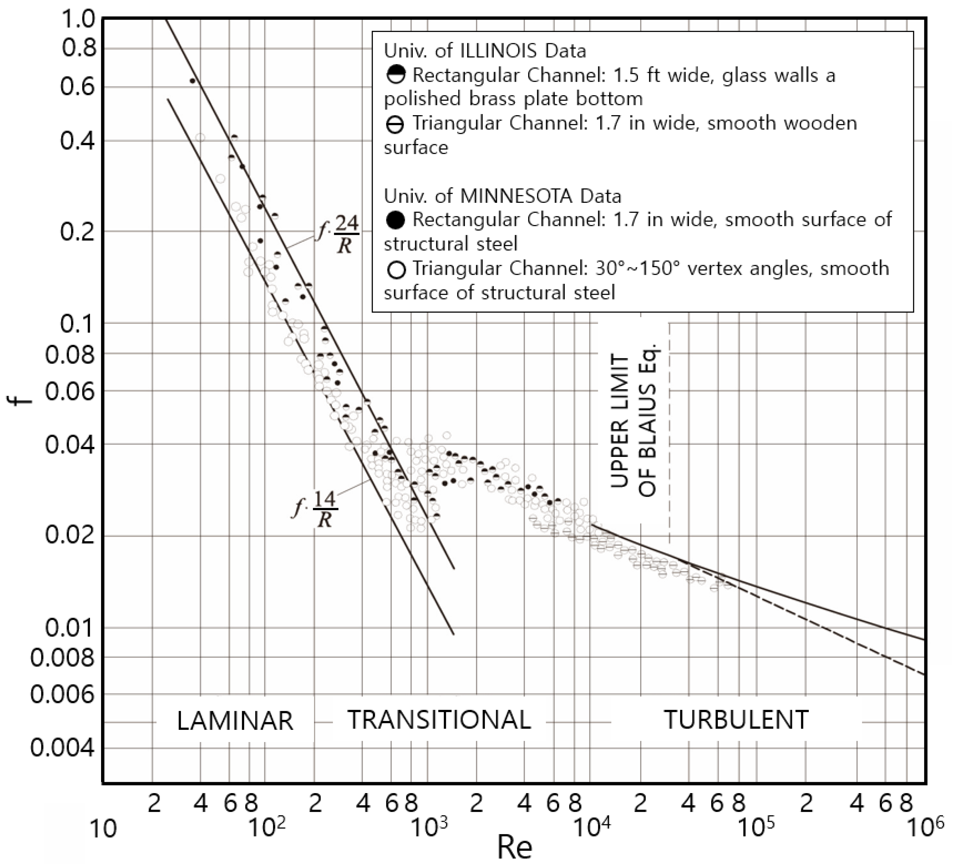
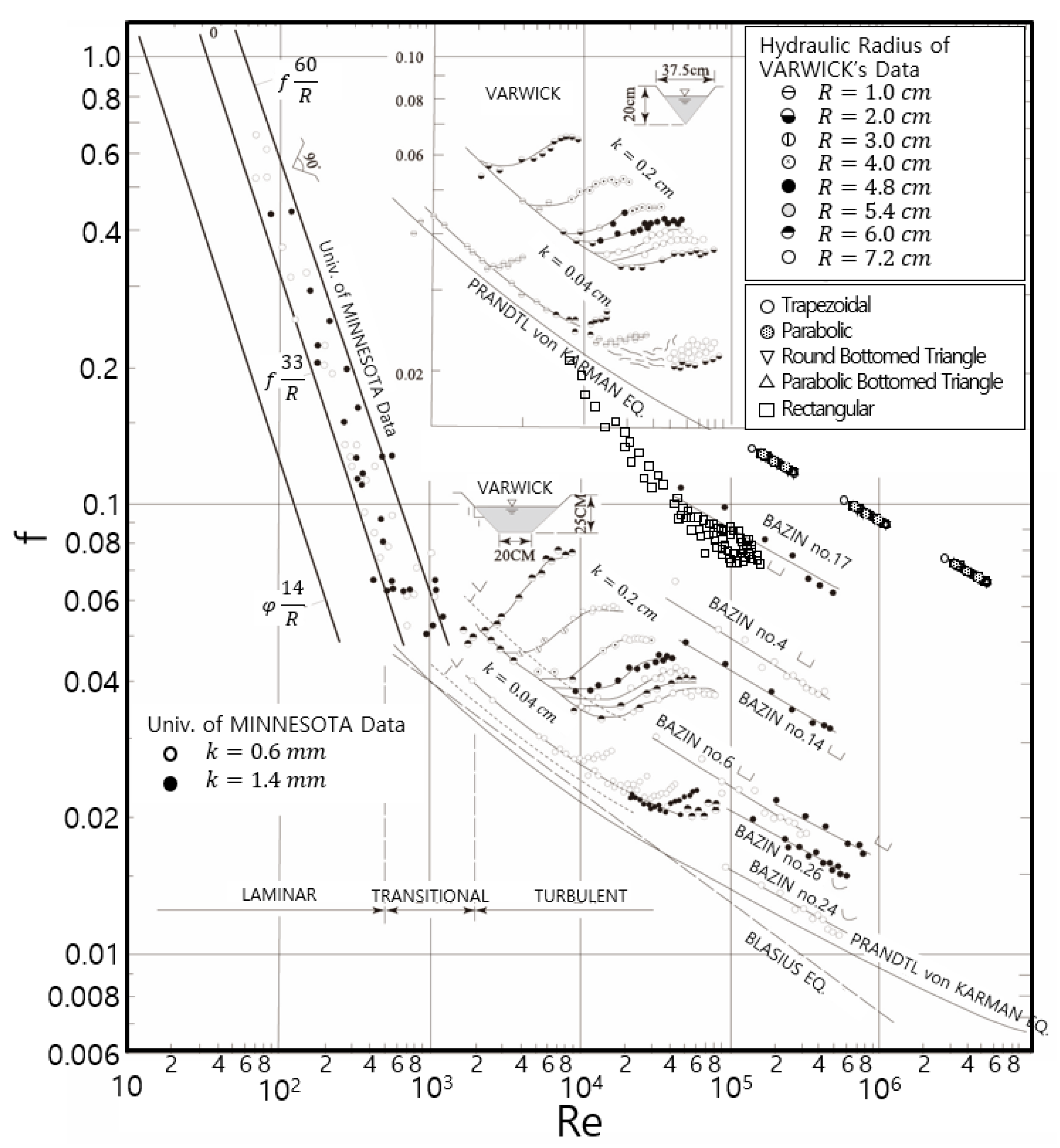
Therefore, it is possible to establish a relationship between and by an experiment in an open-channel flow using the above equations. However, the relation factors to are different between the open-channel flow and the pipe flow, because it is affected by multiple factors, such as free water surfaces in the waterways, hydraulic radius, and water surface slope. Figure 1 shows the relationship between smooth and rough channel flows by analyzing various overseas experimental data [17].
The shortcomings of the above studies are that it is difficult to calculate the energy slopes correctly in an open-channel flow. In addition, equations should be applied differently according to the scope of the . For the example, the Prandtl-von Karman’s equation has to consider an uncertainty when using Equation (3). This is because it is hard to obtain an accurate flow velocity at the bottom of the channel.
2.2. New Friction Coefficient Using Entropy
Shannon [18] first defined entropy by function H(x) and can be written as Equation (6):
where is the probability density function, and is dimensionless but dx has dimension.
Equation (6) means maximizing the entropy that represents the uncertainty for , given for the continuous state variable . Applying this concept to the water velocity can be written as Equation (7):
The following constraints are used, such as the average value and probability, which are available information about which is instantaneous (point) velocity and can be written as Equations (8) and (9):
Arranging the independent constraint conditions can be given as Equation (10):
where is the minimum value of , is the maximum value of , is the constraint number ( is Equation (8) and is Equation (9)).
Therefore, , which maximizes the entropy, can be obtained using the method of Lagrange as Equations (11)–(13):
where .
where and are Lagrange multipliers.
Substituting Equations (12) and (13) into Equation (11) can be constructed as the following Equation (14):
where are the Lagrange multipliers.
Differentiating Equation (14) with respect to results in the velocity as Equation (15):
Equation (15) and (entropy coefficient) are substituted into Equation (8) to obtain Equation (16):
Then Equation (15) and are substituted into Equation (9) to obtain Equation (17) (This is the two-dimensional average velocity equation, which is Chiu’s velocity equation [11,12]):
Equation (17) can be used to restructure Equation (16) to obtain Equation (18):
The shear stress is the product of the dynamic viscosity (kinematic viscosity is the dynamic viscosity divided by density) and the velocity gradient, which can be expressed as Equation (19):
where is the shear stress, is the density of the fluid, is the kinematic viscosity of the fluid, is the mean value of , and is the scale factor, which has the length dimensions.
The shear stress at the channel boundary (bottom) is the shear stress when is , as in Equation (20):
where is the waterway boundary shear stress, is the gravitational acceleration, and is the energy gradient.
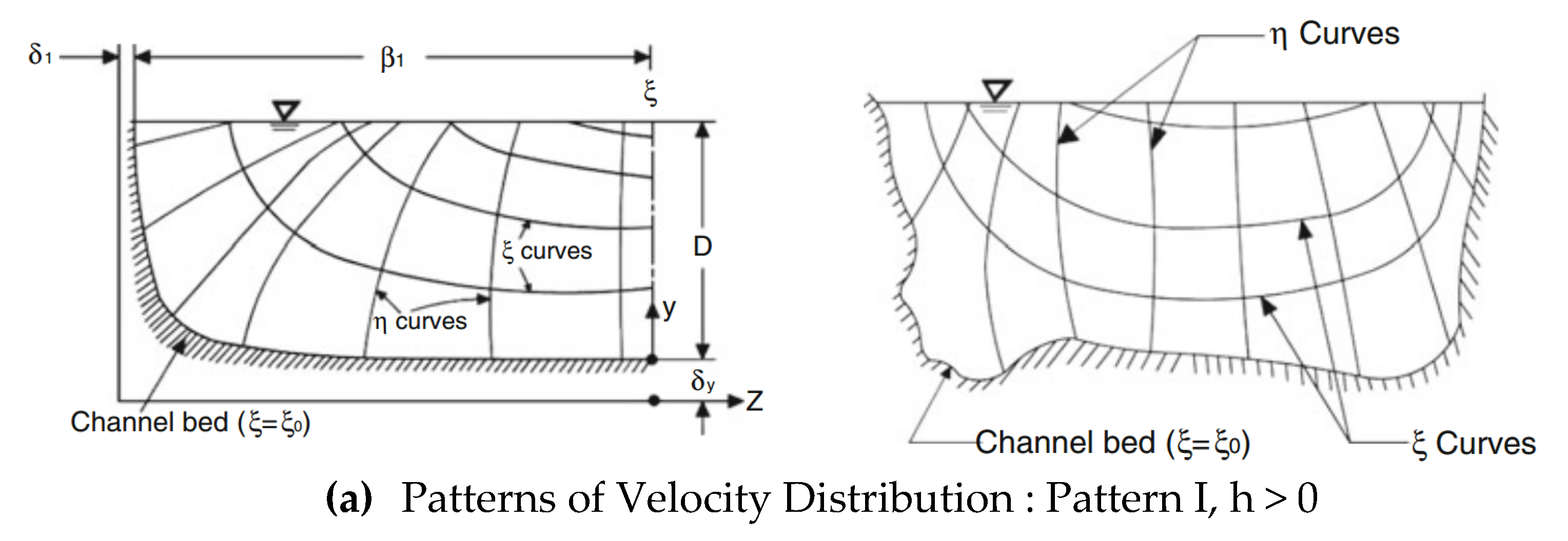
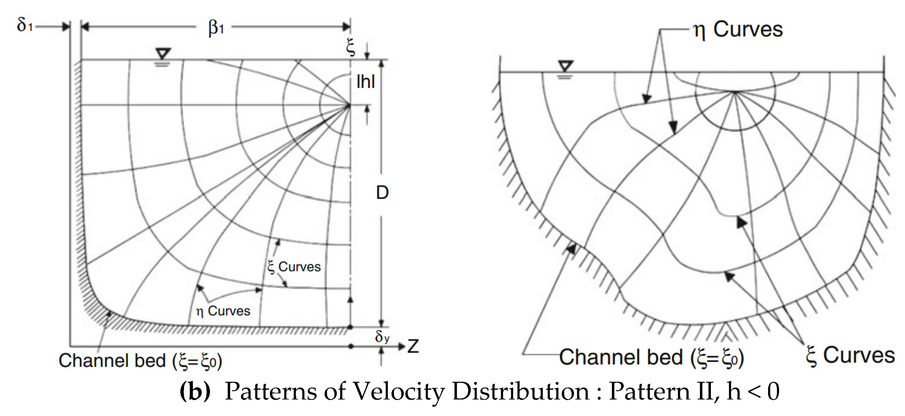
The velocity cumulative probability of is suggested by Chiu [11,12] as Equation (21):
where is the spatial coordinates (), is the velocity at , is the minimum value of (occurring at the channel boundary where ), and is the maximum value of (where is at its maximum (i.e., )) (see Figure 2).
The - coordinates are the isovel system, which was first developed by Chiu [11,12] to explain two-dimensional velocity distribution in the cross-section of an open channel.
In Equation (21), if is at the bottom of the channel, is 0 and is 1, and by differentiating the velocity gradient in the channel bed, where , Equation (22) can be obtained:
For a wide channel, can be simplified to and, hence, . For the hydraulic radius, . Therefore, substituting Equation (22) into Equation (20), Equation (23) is obtained:
Equating Equations (18) and Equation (22) expresses the average water velocity in the open-channel flow as Equation (24):
where .
For the friction velocity (), the relationship between the average water velocity and the friction velocity is shown as Equation (25):
To calculate the friction term in Equation (25), Choo’s mean velocity distribution [10] is used for Equation (26):
where .
Choo’s mean velocity was used earlier for calculating the discharge. However, in this paper, it will be used for converting friction velocity, since it has already been modified for the average water velocity in the open-channel flow [10].
The water velocity slope is differentiated from Equation (26), and and are applied as Equation (27):
where, because the bottom boundary layer , Equation (27) is equal to Equation (28):
Equation (28) is inserted into Equation (20), which is the shear stress at the channel boundary, to obtain Equation (29):
The relationship between the average water velocity and the friction velocity of the friction loss coefficient of the pipe flow is shown in Equation (30):
Equations (25) and (30) are substituted into Equation (29) to obtain Equation (31):
Therefore, if Equation (31) is substituted for Equations (24) ( and (26) ( and use , Equation (32) can be obtained:
Equation (32) can be used to estimate the frictional loss coefficient (f) of the open-channel flow, which reflects its entropy. Equation (32) does not require the hydraulic factors used in the existing equations, such as shear velocity () or energy gradient (). In addition, the friction loss coefficient () can be expressed with only the average water velocity and the entropy , which are easy to obtain. In addition, there is also an advantage in that the energy gradient () can be estimated by using Equation (32).
Therefore, in this study, we proposed the friction loss coefficient of Equation (32) in the open-channel flow by using the concept of entropy, which has been used in many fields recently. The data used to demonstrate the utility of the equation were obtained by Yuen [19] and Babaeyan-Koopaei [20] for each stream of water. It is shown in the Figure 1 that the estimated friction loss coefficient was compared with the measured friction loss coefficient.
3. Experimental Data
To evaluate the accuracy of the proposed equation, we calculated the friction coefficient based on the data measured at the rectangular channel. The estimated results were compared with the measured data, as shown in Figure 1. First, the data measured by Yuen [19] at the trapezoidal section were used. Then, the data were measured by Babaeyan-Koopaei [20] at the trapezoid, the parabolic round-bottomed triangle, and the parabolic-bottomed triangle trapezoidal channel.
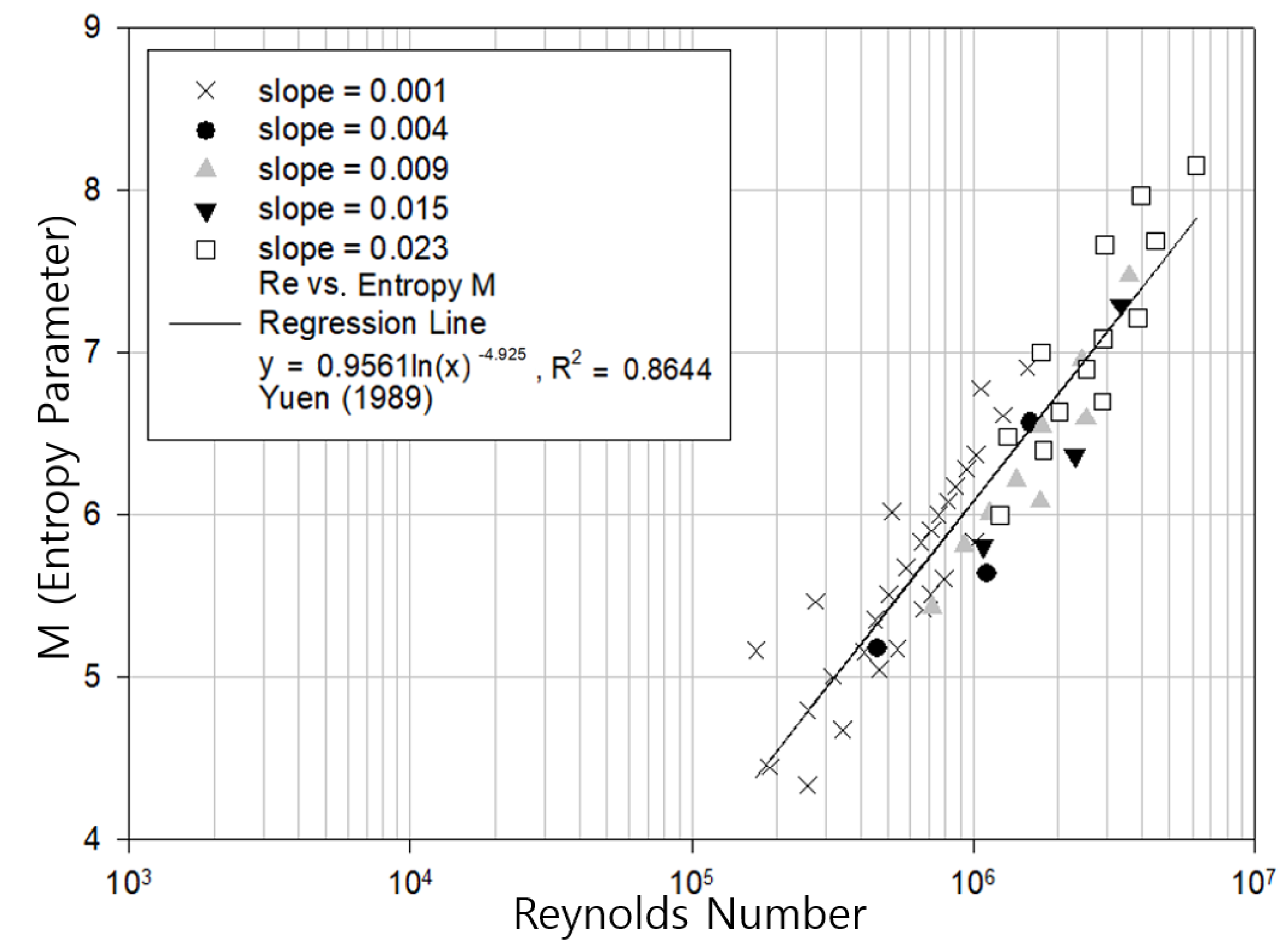
Yuen obtained data in a fully developed turbulent flow of the smooth trapezoidal open-channel flow. The ranges of the data were , and (where was the aspect ratio). The subcritical flow was also studied for the compound trapezoidal channel, which ranged in depths of . Here, Dr is the relative depth ratio ( where is the flow depth of the channel, and is the depth of the lower main channel). Several series of experiments were undertaken by using the Preston tube technique. These experiments were performed in a 21.26-m-long tilting channel with a working cross-section of 0.615 m wide 0.365 m deep. A total of three sets were measured under the equivalent conditions, varying the bed slope at 0.001, 0.004, 0.009, 0.015, and 0.023. In addition, the point velocities were measured across the whole cross-section for the selected flow depths. Particular attention was focused on understanding the Reynolds and Froude number effects on these distributions.
Babaeyan-Koopaei [20] measured the data in the trapezoidal, parabolic, round-bottomed triangle, and parabolic-bottomed triangle channel. For each section, the measured data were used with the changes in the flow velocity and water levels under three flow conditions: , , and (see Babaeyan-Koopaei for more information).
The values of the measured Re data are shown in Table 1. It can be seen that the measured data in the rectangular section reflected the transition zone and the turbulence zone. In the trapezoidal, parabolic, round-bottomed triangle, and parabolic-bottomed triangle sections, the measured data reflected the full turbulence zone.
4. Estimation of the Entropy Parameter, M
An estimate of the entropy parameter is needed to use Equation (29). For the estimation of entropy parameter M, most researches used Equation (15) to calculate the entropy parameters in which the equation required, essentially, the maximum flow velocity in an open channel.
However, the maximum velocity occurred at the center of the pipe flow, but the location of the maximum velocity was unclear at the open-channel flow. Additionally, a lot of manpower, time, and effort were required to measure the maximum velocity in the open-channel flow. Moramarco [21] calculated the values by using Equation (15). For that, he used data obtained from the average and maximum velocities at the upper river basin. Moramarco [22] proposed an equation for calculating by substituting Chiu’s theory and the Manning and Prandtl-von Karman equations. However, the disadvantage of these equations were that it was difficult to clearly identify the point where the maximum velocity occurred, , and imaginary distance, , where the velocity was zero in the riverbed.
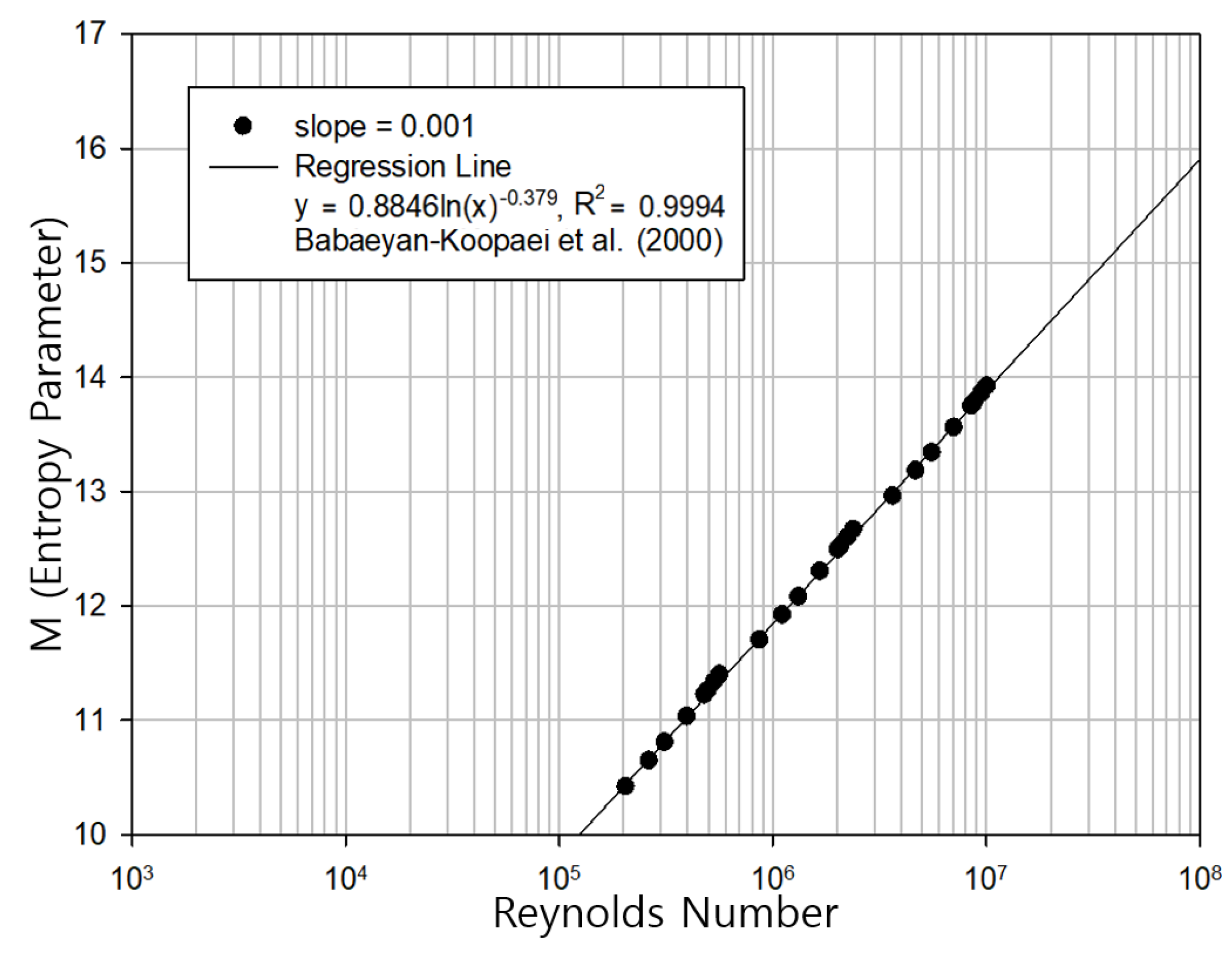
This study determined the entropy parameter by using the expression developed by Choo [23]. The advantage of this method was that the entropy parameters in the stream could be obtained at any time without using the uncertain maximum velocity.
The entropy parameters and the were calculated by using the same characteristics as those shown in Figure 3 and Figure 4. As the entropy parameter, was increased, and the was also increased. On the other hand, as the friction coefficient increased, decreased. Based on the value of , the two flows were identified as turbulent flows.
5. Results Analysis
The entropy parameter M, defined in Section 4, was used in Equation (32) to calculate the coefficient of friction in an open-channel flow. The relationship between and is shown in Figure 5 and Figure 6.
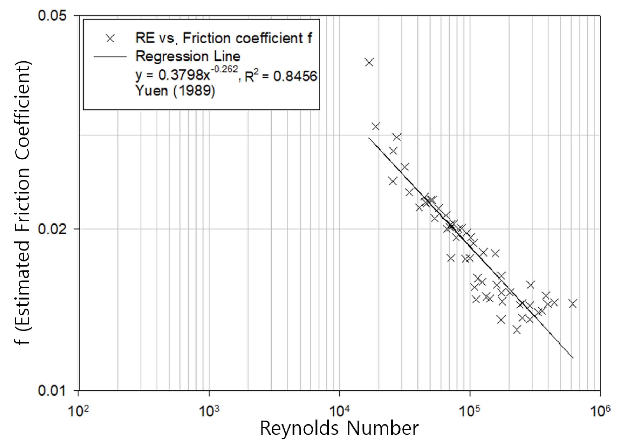
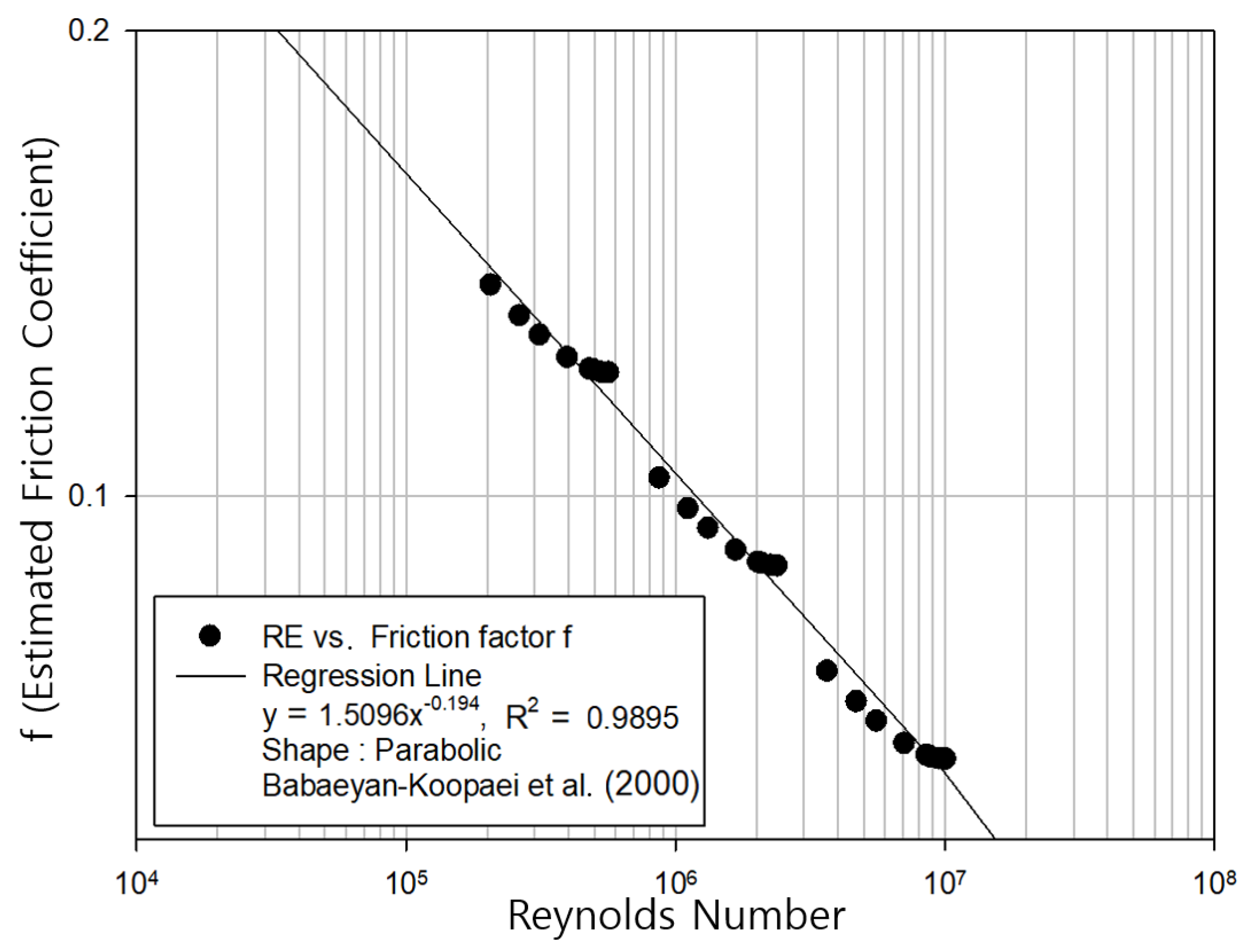
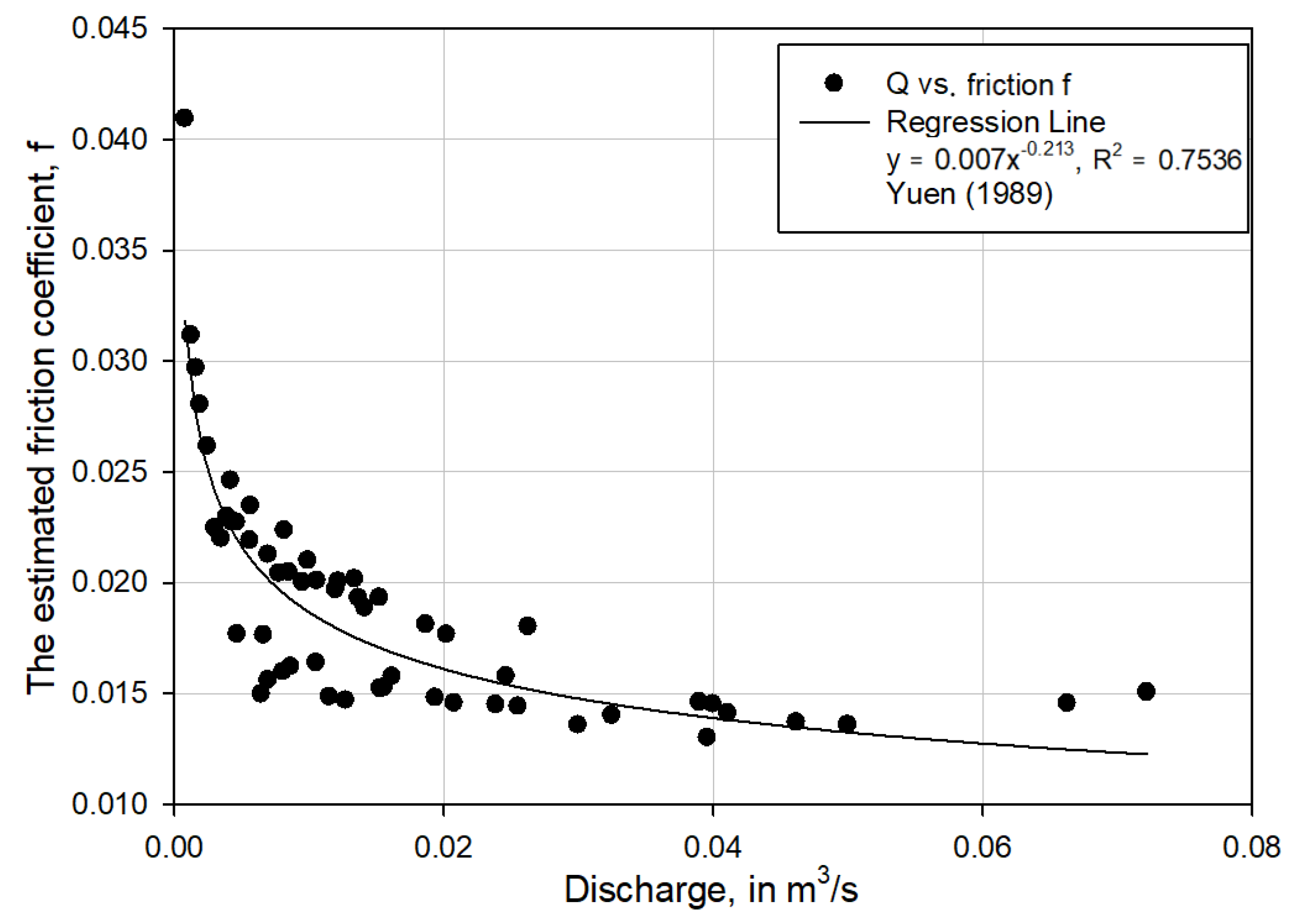
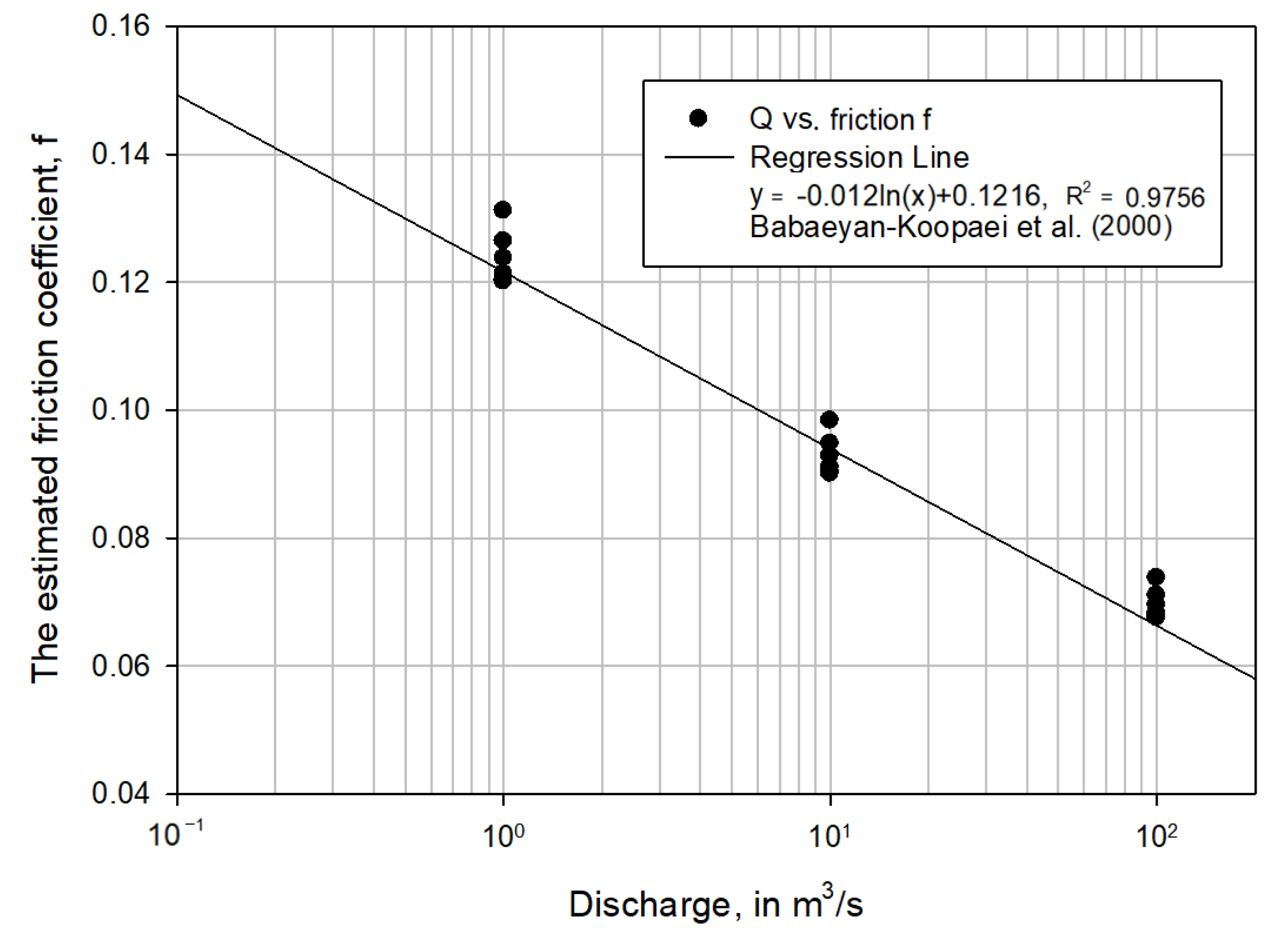
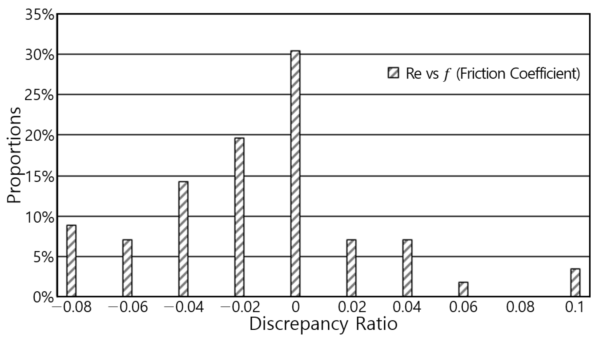
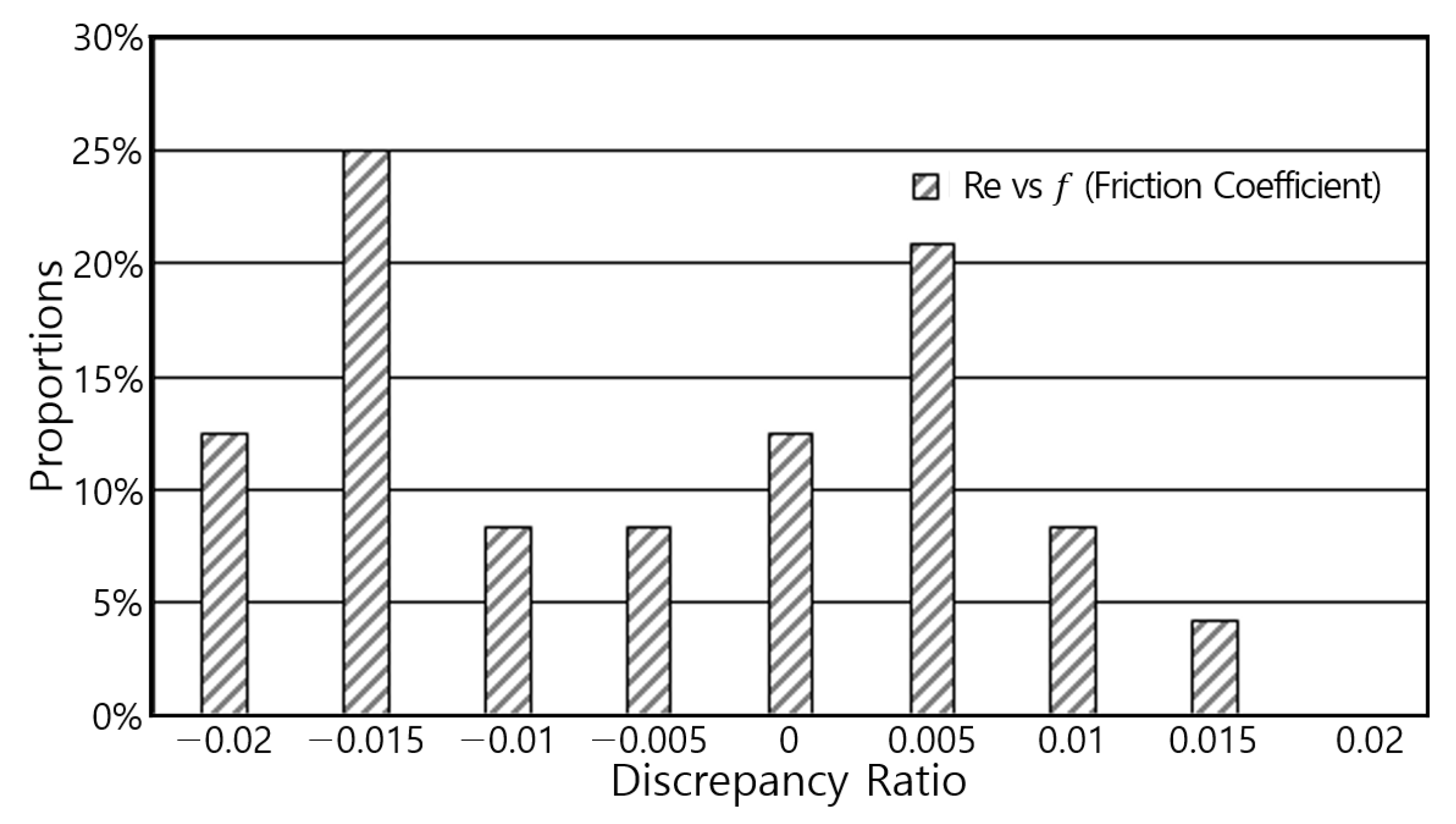
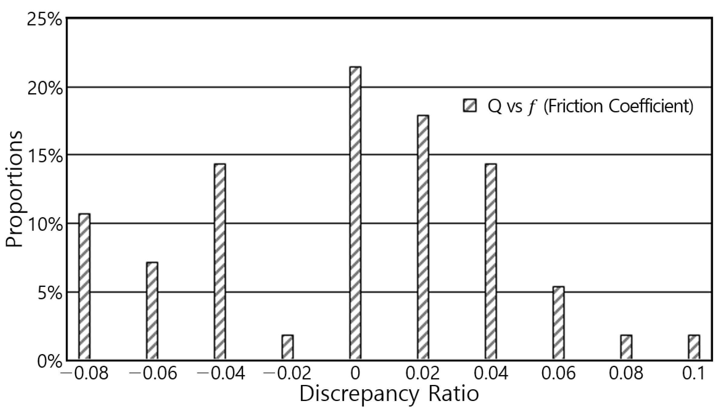
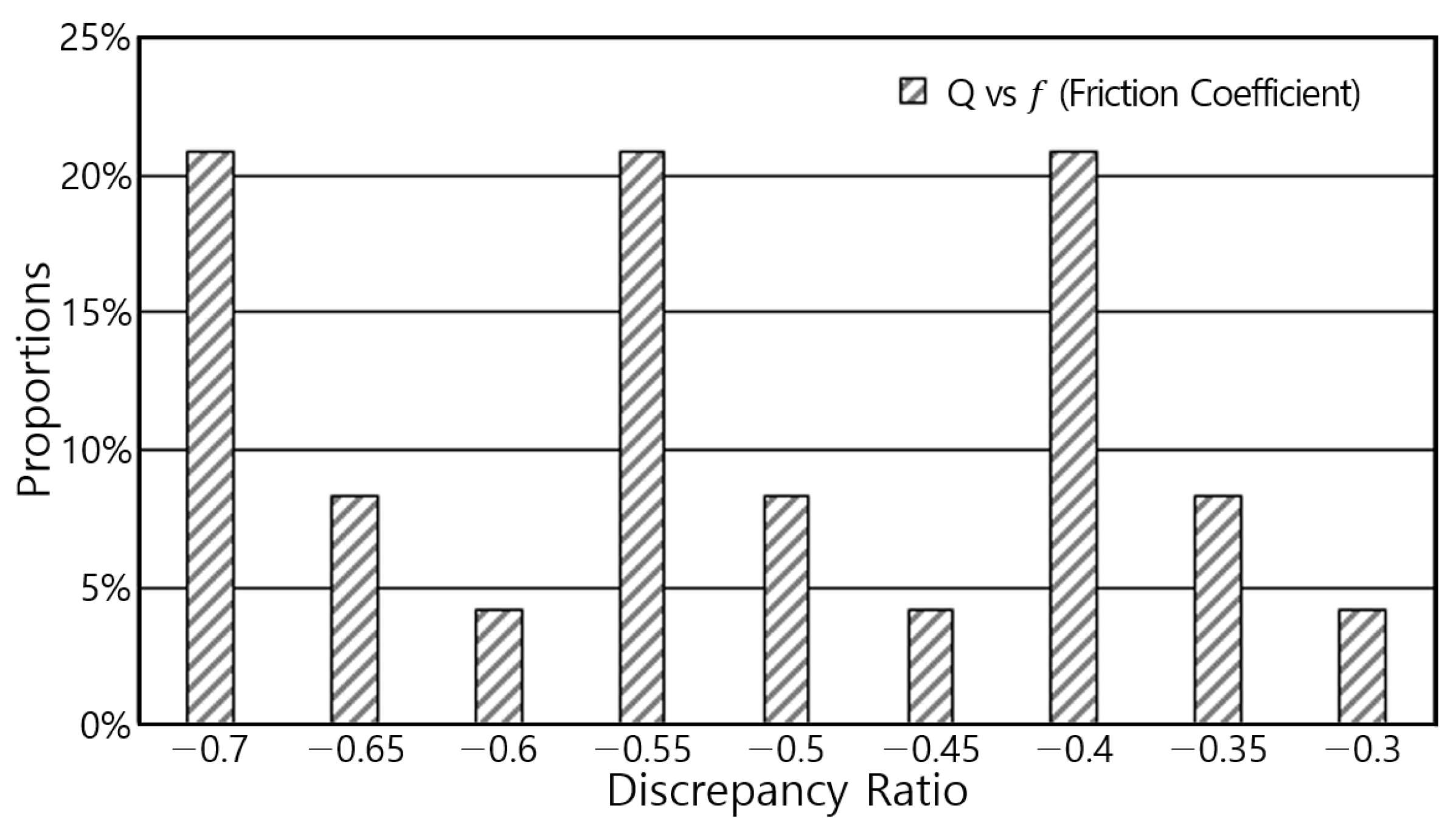
The coefficient of friction f in Figure 5 and Figure 6 shows the same trend as in Figure 1, where f tends to decrease as Re increases. In addition, in Figure 7 and Figure 8, the friction coefficient, , shows a tendency to decrease as the discharge increases. The discrepancy ratio is the error ratio between the measurement and calculated values, separated by a range. The proportions on the y-axis are the ratio of the total comparison quantity to the range of the x-axis. Figure 9, Figure 10, Figure 11 and Figure 12 show that the discrepancy ratio results of the proposed equation were all distributed near 0.
The above results are summarized as follows: The entropy parameter is a linear function of which is an increasing function of . The friction coefficient f is a linear decreasing function of which is a decreasing function of . Figure 13 shows the above results calculated using the proposed Equation (32), along with the relationship between the friction coefficients and . Comparing the scale with a previous empirical study resulted in rough flows; the coefficient of determination was observed to be 0.8 within the range of the flow of the rectangular channel and 0.75 within the range of the flow of the compound trapezoidal channel.
Figure 10 shows the results determined with Yuen’s data measured in the rectangular and trapezoidal channels. Particularly, the calculated value was expressed as , which exceeded the existing value. This range means that the proposed equation can represent the actual phenomenon in the natural stream.
The picture on the right shows the results determined with Babaeyan-Koopaei’s data measured in the trapezoidal, parabolic, round-bottomed triangle, and parabolic-bottomed triangle channels. In this case, the calculated value was expressed as , which was close to the maximum range of the previous value. The important thing is that even the compound trapezoidal sections that were similar to the natural section, which were not available in the existing graph, as shown in Figure 1, can easily be calculated for and . In Table 2 and Table 3, the regression equations from the Yuen [19] and Babaeyan-Koopaei [20] data show the relationship between , , , and .
Comparing the scale with a previous empirical study results in rough flows; the coefficient of determination was observed to be 0.8 within the range of the flow of the rectangular channel and 0.75 within the range of the flow of the compound trapezoidal channel.
As can be seen in Figure 13, the values of the coefficient of friction determined from past experiences are properly correlated with the measured data. There is no bouncing value on the graph. For the rectangular channel, this seems expressed fairly well as Bazin no. 17. Other types of channels matched well with the extended lines of the Prandtl-von Karman equation. In other words, it is meaningful that the values of the friction coefficient determined from proposed equation can be accurately estimate based on a theoretical formula rather than on an empirical parameter under a number of conditions.
6. Conclusions
The results of a study conducted approximately 100 years ago are still used to estimate the friction coefficient in an open-channel flow. However, as with the pipe flow (perfusion), the friction coefficient must be correctly determined in order to interpret the correct flow. This paper proposes a new form of friction coefficient calculation by using the two-dimensional velocity formula of Chiu [11,12] and probabilistic entropy.
The advantage of this equation is that it eliminates the terms of energy slopes, which are difficult to measure or calculate in an open-channel flow, making their application simple and very accurate on a theoretical basis.
In uniform flow conditions, a channel bed gradient may be the same or almost the same as an energy slope or water surface gradient. The normal depth is maintained as long as the slope, cross-section, and the surface roughness of the channel remains unchanged; thus, the average flow velocity remains constant. However, in natural flow and human-made open channels, such as irrigation systems and sewer lines, there are mostly nonuniform or unsteady flows. Unlike uniform flow conditions, these varied flows do not share the same energy slope, bed gradient, and water surface gradient.
Based on the data measured in the rectangular section, the proposed equation was used to determine the entropy parameter and the friction coefficient . The induced entropy parameters were shown to be a linear function of and the friction coefficient was the decreasing function of .
If this study is to be carried out continuously by hydraulic data measured in various channel shapes, laboratory channels, and natural streams, the friction coefficient value estimated from the proposed equation will be actively used in the flow analysis and the design of hydraulic structures.
Author Contributions
Y.-M.C. and S.-H.P. carried out the survey of the previous studies. Y.-M.C. wrote the manuscript. S.-H.P. conducted all the simulations. Y.-M.C., J.-G.K., and S.-H.P. conceived the original idea of the proposed method. All authors have read and agreed to the published manuscript.
Funding
This research was funded by the Institute of Industrial Technology, Pusan National University.
Institutional Review Board Statement
Not applicable.
Informed Consent Statement
Not applicable.
Acknowledgments
This research was supported by the Institute of Industrial Technology, Pusan National University.
Conflicts of Interest
The authors declare no conflict of interest.
References
- Darcy, H.; Bazin, H. Recherches Hydrauliques; Enterprises par M.H. D’Arcy; Imprimerie Nationale: Paris, France, 1865. [Google Scholar]
- Yu, K.K. Particle Tracking of Suspended-Sediment Velocities in Open-Channel Flow. Ph.D. Thesis, Civil and Environmental Engineering, University of Iowa, Iowa City, IA, USA, 2004. [Google Scholar]
- Bazin, H.E. Recherches Experimentales sur Lecoulement de Leau dans les Canaux Decouverts; Memoire Presentes par Divers Savants al Academie des Sciences: Paris, France, 1865. [Google Scholar]
- Bazin, H.E. Etude d’une nouvelle formule pour calculer le debit des canaux decouverts. In Annales des Ponts et Chaussées; P. Vicq-Dunod: Paris, France, 1897; Volume 14, pp. 20–70. [Google Scholar]
- Varwick, F. Zur Fließformel für offene Künstliche Gerinne; Dresden University: Dresden, Germany, 1945. (In German) [Google Scholar]
- Manning, R.; Griffith, J.P.; Pigot, T.F.; Vernon-Harcourt, L.F. On the Flow of Water in Open Channels and Pipes; Transaction of the Institution of Civil Engineers of Ireland: Dublin, Ireland, 1890; Volume 20. [Google Scholar]
- Ganguillet, E.; Kutter, W.R. An investigation to establish a new general formula for uniform flow of water in canals and rivers. Z. Oesterreichischen Ing. Archit. Ver. 1869, 21, 6–25. [Google Scholar]
- Chezy, A. Thesis on the Velocity of the Flow in a Given Ditch; des Ponts et Chaussees, Library in France: Paris, France, 1775; Volume 847. [Google Scholar]
- Chow, V.T. Open-Channel Hydraulics; Mcgrow-Hill Civil Engineering Series; McGraw-Hill: Tokyo, Japan, 1959. [Google Scholar]
- Choo, T.H.; Yoon, H.C.; Lee, S.J. An estimation of discharge using mean velocity derived through Chiu’s velocity equation. Environ. Earth Sci. 2013, 69, 247–256. [Google Scholar] [CrossRef]
- Chiu, C.L. Velocity distribution in open channel flow. J. Hydraul. Eng. 1988, 115, 576–594. [Google Scholar] [CrossRef]
- Chiu, C.L. Application of entropy concept in open-channel flow study. J. Hydraul. Eng. 1991, 117, 615–628. [Google Scholar] [CrossRef]
- Blasius, H. Das Ähnlichkeitsgesetz bei Reibungsvorgängen in Flüssigkeiten; Forschungsheft des Vereins Deutscher Ingenieure: Berlin, Germany, 1913; Volume 131. [Google Scholar]
- Kảrmản, T. Mechanische Ähnlichkeit und turbulenz. In Proceedings of the 3rd International Congress for Applied Mechanics, Stockholm, Sweden, 24–29 August 1930; Volume 1, pp. 85–93. [Google Scholar]
- Prandtl, L. >The Mechanics of Viscous Fluids; Durand, B., Ed.; Aerodynamic Theory Springer: Berlin, Germany, 1935; Volume III, division G. 142. [Google Scholar]
- Nikuradse, J. Gesetzmassigkeiten der turbulenten Stromung in glatten Rohren; Ver Deutsch. Ing. Forschungsheft: Berlin, Germany, 1932; Volume 356. [Google Scholar]
- Ryu, H.J.; Kim, J.H.; Lee, B.H.; Lee, W.H.; Jang, I.S. Choisin Hydrography; Donghwa, Korea, 2007. [Google Scholar]
- Shannon, C.E. A mathematical theory of communication. Bell Syst. Tech. J. 1948, 27, 379–423. [Google Scholar] [CrossRef] [Green Version]
- Yuen, W.H. A Study of Boundary Shear Stress, Flow Resistance and Momentum Transfer in Open Channels with Simple and Compound Trapezoidal cross Section. Ph.D. Thesis, Department of Civil Engineering, University of Birmingham, Birmingham, UK, 1989. [Google Scholar]
- Babaeyan-Koopaei, K.; Valentine, E.M.; Swailes, D.C. Optimal design of parabolic-bottomed triangle canals. J. Irrig. Drain. Eng. 2000, 126, 408–411. [Google Scholar] [CrossRef]
- Moramarco, T.; Saltalippi, C.; Singh, V.P. Estimation of mean velocity in natural channels based on Chiu’s velocity distribution equation. J. Hydrol. Eng. 2004, 9, 442–450. [Google Scholar] [CrossRef]
- Moramarco, T.; Singh, V.P. Formulation of the entropy parameter based on hydraulic and geometric characteristics of river cross sections. J. Hydraul. Eng. 2010, 15, 852–858. [Google Scholar] [CrossRef]
- Choo, Y.M.; Yun, G.S.; Choo, T.H.; Kwon, Y.B.; Sim, S.Y. Study of shear stress in laminar pipe flow using entropy concept. Environ. Earth Sci. 2017, 76, 1–27. [Google Scholar] [CrossRef]
Figure 1.
Relationship between f and Re for smooth channels (Flow conditions: Laminar, Transitional, and Turbulent [14]).
Figure 1.
Relationship between f and Re for smooth channels (Flow conditions: Laminar, Transitional, and Turbulent [14]).


Figure 3.
Relationship between and calculated using Yuen’s data.

Figure 4.
Relationship between and calculated using Babaeyan-Koopaei’s data.

Figure 5.
The relationship between and calculated using Yuen’s data.

Figure 6.
The relationship of and calculated using Babaeyan-Koopaei’s data.

Figure 7.
The relationship of and calculated using Yuen’s data.

Figure 8.
The relationship of and calculated using Babaeyan-Koopaei’s data.

Figure 9.
The discrepancy ratio for and calculated using Yuen’s data.

Figure 10.
The discrepancy ratio for and calculated using Babaeyan-Koopaei’s data.

Figure 11.
The discrepancy ratio for and calculated using Yuen’s data.

Figure 12.
The discrepancy ratio for and calculated using Babaeyan-Koopaei’s data.

Figure 13.
The comparison between the empirical and calculated friction coefficients using Yuen and Babaeyan-Koopaei (rough channel).
Figure 13.
The comparison between the empirical and calculated friction coefficients using Yuen and Babaeyan-Koopaei (rough channel).


Table 1.
The range of Reynolds numbers with the cross-section shape and the channel slope.
| Data | Cross-Section Shape | Channel Slope | Reynolds Number Range |
|---|---|---|---|
| Yuen [19] | Rectangular | 0.001 | 16,920~156,400 |
| 0.004 | 45,770~160,900 | ||
| 0.009 | 71,450~358,000 | ||
| 0.015 | 108,600~335,000 | ||
| 0.023 | 124,400~618,300 | ||
| Babaeyan-Koopaei [20] | Trapezoidal | 0.001 | 167,000~4,474,000 |
| Parabolic | 0.001 | 135,000~4,630,000 | |
| Round-bottomed triangle | 0.001 | 167,000~4,684,000 | |
| Parabolic-bottomed triangle | 0.001 | 167,000~4,630,000 |
Publisher’s Note: MDPI stays neutral with regard to jurisdictional claims in published maps and institutional affiliations. |
© 2021 by the authors. Licensee MDPI, Basel, Switzerland. This article is an open access article distributed under the terms and conditions of the Creative Commons Attribution (CC BY) license (https://creativecommons.org/licenses/by/4.0/).
Share and Cite
MDPI and ACS Style
Choo, Y.-M.; Kim, J.-G.; Park, S.-H. A Study on the Friction Factor and Reynolds Number Relationship for Flow in Smooth and Rough Channels. Water 2021, 13, 1714. https://doi.org/10.3390/w13121714
AMA Style
Choo Y-M, Kim J-G, Park S-H. A Study on the Friction Factor and Reynolds Number Relationship for Flow in Smooth and Rough Channels. Water. 2021; 13(12):1714. https://doi.org/10.3390/w13121714
Chicago/Turabian StyleChoo, Yeon-Moon, Jong-Gu Kim, and Sang-Ho Park. 2021. "A Study on the Friction Factor and Reynolds Number Relationship for Flow in Smooth and Rough Channels" Water 13, no. 12: 1714. https://doi.org/10.3390/w13121714
Note that from the first issue of 2016, this journal uses article numbers instead of page numbers. See further details here.