Discharge Calculation of Side Weirs with Several Weir Fields Considering the Undisturbed Normal Flow Depth in the Channel

Abstract

Discharge behavior at side weirs is significantly influenced by the water surface profile along the weir crest. In the past century, different approaches were developed to describe this profile and the associated discharge coefficients. However, the application of these methods to practical problems poses a particular challenge, as a complex three-dimensional funnel is formed due to the discharge reduction, leading to significant uncertainties in determining the relevant flow depth. For this reason, a new approach for the determination of the discharge coefficient of side weirs was developed that refers to the undisturbed normal flow depth in the main channel. Based on a comprehensive parametric study utilizing 3D-numerical simulations, the influence of the weir and channel characteristics on the discharge behavior at the side weir was analyzed. A revised formula for estimating the discharge coefficient for side weirs with multiple weir fields was derived using multiple regression analyses. Validation of the numerical simulations was carried out by applying a physical scale model, showing good agreement between the results.

1. Introduction

1.1. Discharge Behaviour at Side Weirs in the Context of Flood Risk Management

Side weirs are hydraulic structures used to divert water from the main channel in flooding, agricultural, sewage, and urban runoff applications. In the context of flooding, side weirs are used in rivers where effective flood mitigation requires discharge diversion into an attached channel or retention basin. Through the targeted filling of the retention basin, the flood peak discharge can be significantly reduced. However, early or unnecessary discharge reductions can reduce mitigative retention capacity of the basin, hindering the efficacy of the system [1]. To exploit the full retention capacity of the mitigation system, weir discharge regulation is crucial. Due to the typically lateral arrangement of these basins to the river, inlet structures need to be aligned parallel to the main flow direction in the channel and thus represent a lateral weir. Therefore, the discharge behavior is mainly influenced by prevailing flow depth, weir crest length, and a specific discharge coefficient [2]. In the case of an uncontrolled weir with a fixed crest height and weir length, the weir discharge results as a function of the prevailing flow depth. For a controlled weir with multiple weir fields regulated by sluice gates, weir discharge can be adjusted by the number of open gates, representing the effective weir length. In order to control and adjust this system, reliable flow depth and discharge measurements are required that reflect current flood conditions, but they are unaffected by the impact of discharge reduction on the water surface.

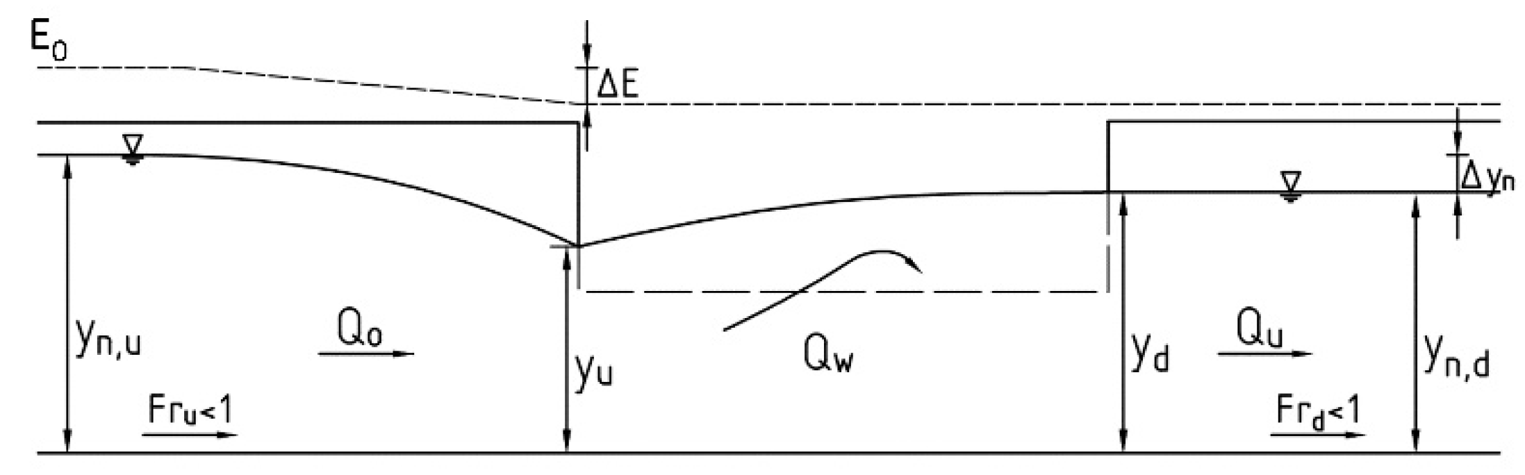
1.2. Theoretical Background

Side weir discharge analysis has been the focus of many researchers, with De Marchi [2] introducing one of the first analytical, rational approaches to calculate the discharge coefficient. The introduced methods and assumptions have served as the framework to further develop evaluation methods for the discharge of side weirs [3,4,5,6,7,8]. However, variations in channel geometry, weir type, and hydraulic conditions have made a standardized approach difficult to develop, inspiring additional investigations [9,10,11,12,13]. Uyumaz and Muslsu [14] provided insights into the flow over a side weir in a circular channel considering both the subcritical and supercritical flow. They developed procedures for determing the discharge coefficent for both flow states utlizing energy relationships. It was observed that flow behavior in front of the weir presented in the same manner as in a rectangular channel assuming constant specific energy in both flow regimes. Citing the complexity of evaluating side weir flow, Castro-Orgaz and Hager [15] contributed an evaluation method based on applying the momentum and energy equations in both streamwise and transverse directions, considering a prismatic channel and a rectangular sharp-crested weir. They concluded that the momentum approach provides superior results given the uncertainties when applying the energy equation, and that the effects of velocity distribution are significant. Crispino et al. [16] investigated supercritical flow conditions, which are not ideal for side weirs, using a low-crested bilateral weir. Their research addressed non-optimal hydraulic conditions that may be present in poorly designed hydraulic devices. They found that predicting hydraulic parameters considering the available theoretical methods proved unreliable, given the flow state and weir type. To address this, both momentum and energy conservation approaches were applied to evaluate side weir hydraulics. In this application, the energy conservation approach provided reasonable accuracy, while the momentum approach required the correct estimation of multiple parameters.

The mentioned authors have provided substantial advancements in evaluating side weir discharge given a range of hydraulic and geometric conditions. However, further research is required considering multiple, adjustable weir fields being initially closed, and opening in response to necessary flood mitigating discharge reductions, representing conditions and systems found in nature. For this purpose, the discharge behavior of the lateral weir is initially considered in this study based on a simplified one-dimensional approach. Assuming subcritical discharge conditions with a normal depth y_n,u upstream of the weir, the discharge reduction at the side weir leads to a reduction in the normal depth y_n,d at the downstream end of the weir. Applying a one-dimensional approach, the flow depth decreases continuously from the upstream normal depth (y_n,u) to the upstream end of the weir (Figure 1).

With the assumption of a constant specific energy head along the weir, the flow reduction at subcritical flow conditions leads to an increasing flow depth. This behavior can be described with the one-dimensional equation of a spatially varied flow, with non-uniform discharge in the channel, which is based on the theoretical principle of energy conservation (Equation (1)) [1,17]:

$$\frac{\mathrm{d}y}{\mathrm{d}x}=\frac{{\mathrm{I}}_{\mathrm{S}}-{\mathrm{I}}_{\mathrm{E}}+\frac{\mathsf{\alpha }\times \mathrm{q}\times {\mathrm{Q}}_x}{\mathrm{g}\times {\mathrm{A}}^2}}{1-\frac{\mathsf{\alpha }\times \mathrm{B}\times {\mathrm{Q}}_x}{\mathrm{g}\times {\mathrm{A}}^3}}$$

(1)

where A is the wetted cross-sectional area, B is the water surface width, g is the acceleration due to gravity, Q_x is the discharge in the channel at position x along the weir, q is the weir discharge per unit length, I_S is the channel slope, I_E is the energy slope, dy/dx is the change in flow depth y with x, and α is the energy correction coefficient for non-uniform velocity distribution (α ≥ 1). The weir discharge per unit length can be calculated with the equation according to Poleni [18], taking a discharge coefficient for side weirs (C_Q)and the weir height (w) into account (Equation (2)):

$$\mathrm{q}=-\frac{\mathrm{dQ}}{\mathrm{d}x}=\frac{{\mathrm{dQ}}_{\mathrm{w}}}{\mathrm{d}x}=\frac{2}{3}\times {\mathrm{C}}_{\mathrm{Q}}\times \sqrt{2\mathrm{g}}\times {\left(y-\mathrm{w}\right)}^{\frac{3}{2}}$$

(2)

Weir discharge (Q_W) is realized when Equation (2) is integrated along the weir length L (Equation (3)):

$${\mathrm{Q}}_{\mathrm{w}}=\frac{2}{3}\times {\mathrm{C}}_{\mathrm{Q}}\times \sqrt{2\mathrm{g}}\times {{\displaystyle \int }}_0^{\mathrm{L}}{\left(y\left(x\right)-\mathrm{w}\right)}^{\frac{3}{2}}\mathrm{d}x$$

(3)

With the assumption that the specific energy E₀ remains constant along the weir despite the discharge reduction, approaches based on approximations of the water surface along the weir have been developed for example by De Marchi [2], Schmidt [19], and Dominguez [20]. The common element in these approaches is the need to empirically determine the respective discharge coefficient by means of numerical or physical experiments. Numerous studies have been conducted in past decades, yielding various formulas for estimating these coefficients [2,3,5,6].

Considering real conditions, a complex, three-dimensional water surface funnel is formed around the weir’s inflow area [12,21]. Therefore, in this study, the magnitude of the occurring drawdown, compared to normal flow conditions closely upstream of the drawdown at the weir, was initially investigated by means of a 3D numerical simulation (details on the applied software and model setup are shown in Section 2). Four channel configurations with varying slopes (0.5, 1.0, 1.5, and 2.0‰) were considered, each equipped with the same set of eight weir fields integrated on the orographic left bank. Upstream inflows to the main channel were set so that the same normal flow depth developed in all four cases upstream of the weir drawdown.

In Figure 2 the drawdown of the water surface is shown, making clear that the simplification given in the 1D approach, namely a horizontal water level in a given cross-section, should be questioned. This effect is particularly significant in the upstream region since this water level serves as the main input to most of the weir equations developed so far. A large variation of the water surface is observed, especially in the cross-section at the most upstream weir field. Hence, besides difficulties in actually measuring a surface elevation there, it is unclear which water level in the cross-section is to be considered as being representative. The span of possible water levels to be used obviously leads to a substantial variation of theoretically obtainable weir discharges and deviates from the actual weir outflow. In this context, Di Bacco et al. [9] criticized several papers published in recent years that lacked details on the selected flow depth and misinterpreted the used approaches.

Therefore, an alternative approach was developed in this study using the normal flow depth upstream of the weir drawdown, which in the case of a prismatic channel would correspond to the normal flow depth at the weir when the weir fields are closed. The considered flow depth (pressure head) is similar to the specific energy E₀ when the kinetic energy is small. This is especially the case in regions close to the channel banks. One simple option to estimate the water level is by using standard formulas for open channel flow. By applying Poleni’s equation, the discharge through the weir is calculated as follows (Equation (4)):

$${\mathrm{Q}}_{\mathrm{W}}=\frac{2}{3}\times {\mathrm{C}}_{\mathrm{b}}\times {\mathrm{L}}_{\mathrm{o}}\times \sqrt{2\mathrm{g}}\times {\mathrm{h}}_0{}^{\frac{3}{2}}$$

(4)

where C_b is the mean discharge coefficient representing all open weir fields, L_o is the weir length that is calculated by the number of open weir fields n_o and the weir field width b (Equation (5)):

$${\mathrm{L}}_{\mathrm{o}}={\mathrm{n}}_{\mathrm{o}}\times \mathrm{b}$$

(5)

The average flow depth h₀ is defined with respect to the weir crest height w, which is related to the channel bottom and refers to the normal flow conditions upstream of the drawdown at the weir (Equation (6)):

$${\mathrm{h}}_0=y_0-\mathrm{w}={\mathrm{E}}_0-\mathrm{w}$$

(6)

By transforming Equation (4) and conducting empirical discharge and flow depth measurements, the discharge coefficient C_b can be determined with Equation (7), depending on specific weir and channel characteristics.

$${\mathrm{C}}_{\mathrm{b}}=\frac{{\mathrm{Q}}_{\mathrm{W}}}{\frac{2}{3}\times {\mathrm{L}}_{\mathrm{o}}\times \sqrt{2\mathrm{g}}\times {\mathrm{h}}_0{}^{\frac{3}{2}}}$$

(7)

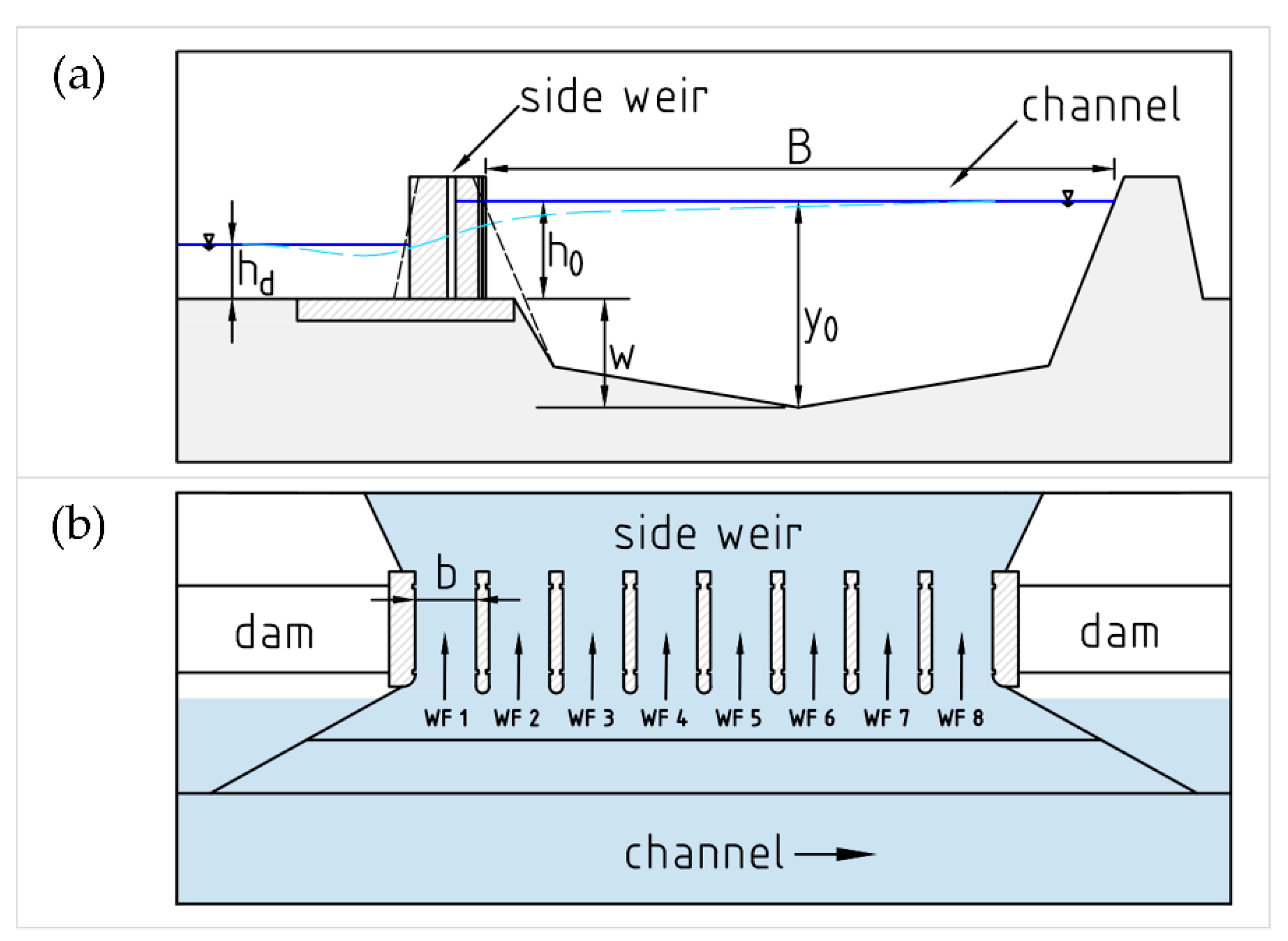
2. Materials and Methods

2.1. Discharge Coefficient

With the aim of deriving a formula for estimating the discharge coefficient C_b (Equation (7)), which is to be used in an equation similar to Poleni’s equation (Equation (4)), a parametric study was carried out using 3D numerical simulations. Besides the obvious local weir geometry, the following parameters characterizing the setup need to be considered: slope of the main channel I_s, weir height w, weir field width b, normal flow depth at undisturbed conditions closely upstream of the weir h₀, flow depth underwater of the weir h_d, the number of open weir fields n_o, and the main channel width B (Equation (8)):

$${\mathrm{C}}_{\mathrm{b}}=\mathrm{f}\left({\mathrm{I}}_{\mathrm{s}},\mathrm{w},\mathrm{b},{\mathrm{h}}_0,{\mathrm{h}}_{\mathrm{d}},n_{\mathrm{o}},\mathrm{B}\right)$$

(8)

Figure 3 shows a sketch of these parameters in a sectional and plan view.

Ensuring standardization, open weir fields were added from up- to downstream. Thus, configurations having one weir field in between the open weir fields (e.g., WF 4) and having one or more upstream weir fields closed (e.g., WF1, WF 2 or WF 3) were not considered. Overall, 103 configurations were analyzed, and the selected range of the respective parameters are summarized in

Table 1. Examined parameters and the selected dimensions.

Parameters	Dimension
Channel roughness kSt	40 (m1/3/s)
Channel slope Is	0.5, 1.0, 1.5, 2.0 (‰)
Froude number Fr at norm flow conditions	0.35, 0.50, 0.65, 0.80 (-)
Channel width B	56, 76, 96, 116 (m)
Flow depth h0	1.6, 2.6, 3.6 (m)
Flow depth underwater of the weir hd	0.0, 0.7*h0, 0.8*h0, 0.9*h0 (m)
Weir field width b	7.0, 15.5, 32.5 (m)
Weir height w	2.2, 4.0, 5.8 (m)
Number of open weir fields no	1–8 (-)

.

In order to derive a formula for estimating the discharge coefficient from the simulation results, dimensionless variables were derived from channel and weir parameters (Equation (9)) by conducting a dimensional analysis (for further details see [22]).

$${\mathrm{C}}_{\mathrm{b}}=\mathrm{f}\left({\mathrm{I}}_{\mathrm{s}},\frac{{\mathrm{h}}_0}{\mathrm{b}\times n_{\mathrm{o}}},\frac{\mathrm{b}\times n_{\mathrm{o}}}{\mathrm{B}},\frac{\mathrm{w}}{{\mathrm{h}}_0},\frac{{\mathrm{h}}_{\mathrm{d}}}{{\mathrm{h}}_0}\right)$$

(9)

The applied multiple linear regression analyses were conducted with the software SPSS, version 24 [23]. The used data were checked to meet the prerequisites of having (i) a linear relationship between the variables, (ii) no outliers, (iii) no autocorrelation, (iv) no multicollinearity, and (v) a normal distribution of the residuals.

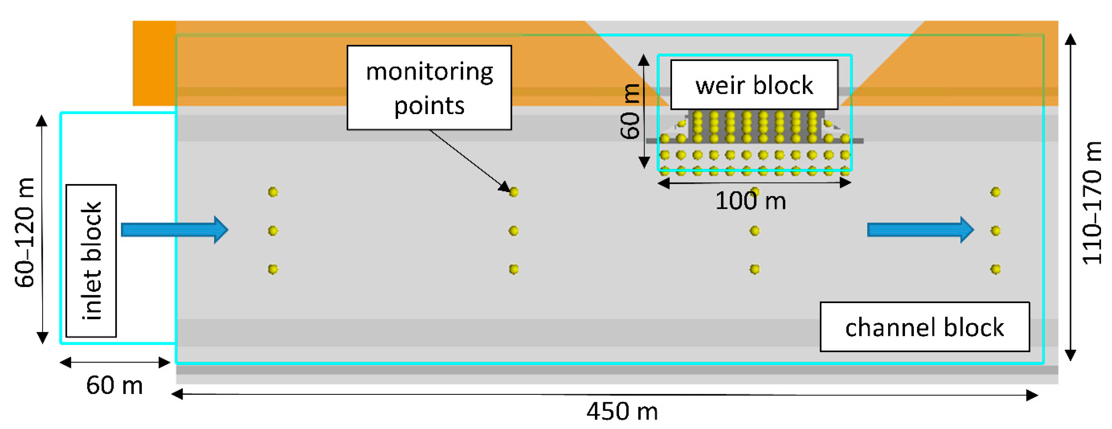
2.2. Numerical Model

The applied software, FLOW-3D^® [24], is widely used and enables modeling of unsteady three-dimensional flows involving complex geometries. The free water level was represented using the volume-of-fluid method according to Hirt and Nichols [25] and the Reynolds-averaged Navier–Stokes equation was solved using the finite difference method on a Cartesian computational grid. The turbulence model used in the simulations was the k-ε model [26].

The numerical model was divided into three mesh blocks (inlet, channel, weir). Since detailed building geometries were considered in the study, an optimized mesh size was required as it determines the degree of spatial resolution. The objective was to represent the channel section under consideration in as much detail as possible. To keep the simulation times at an acceptable level and still have the required accuracy to address the problem, different levels of spatial discretization were tested beforehand. Finally, for the channel and inlet blocks, a non-conforming mesh with an element size x:y:z of 1.0:1.0:0.5 m was used. For the weir, a mesh block was adapted to the surface with a uniform element size of 0.25 m, providing higher resolution in the area of specific interest (Figure 4).

The respective channel discharge was added to the simulation via the inlet mesh block, by applying the boundary condition “volume flow rate”. Using this approach, realistic channel flow conditions can be generated within a short travel distance. The numerical transition from one mesh block to the other occurs via the boundary condition “symmetry”, where flow field variables are transferred along the intersection surface of the mesh blocks, reducing the computational domain, allowing for faster processing, and sparing computer resources.

Outflow characteristics at the downstream end of the channel were controlled by a water level–discharge relationship, which was determined using the Manning–Strickler flow formula with a coefficient of k_St = 40 m^1/3/s. In the numerical model, the equivalent grain roughness was used to describe the channel roughness. Calibration led to a value of k_s = 0.1 m for the channel and k_s = 0.005 m for the weir. For analyzing time series of simulation results, monitoring points and planes were defined in the model setup. In total, 68 monitoring points were defined in 12 cross-sections in the area around the weir and another 12 were defined in the main channel. The discharge was determined both in the channel and in the individual weir fields using measuring baffles.

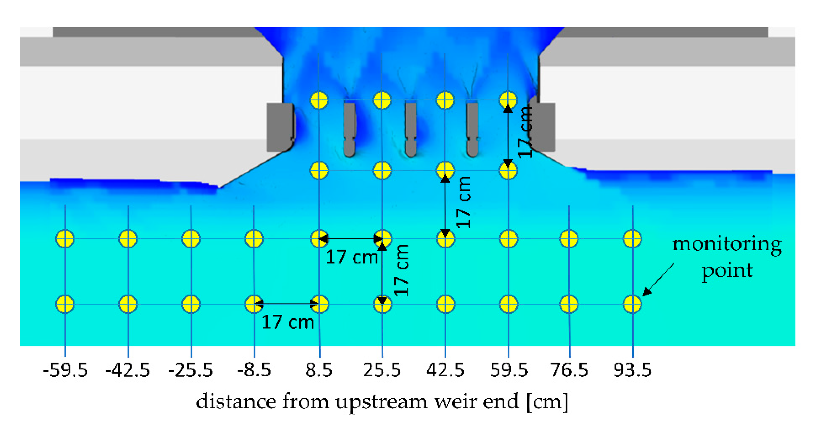
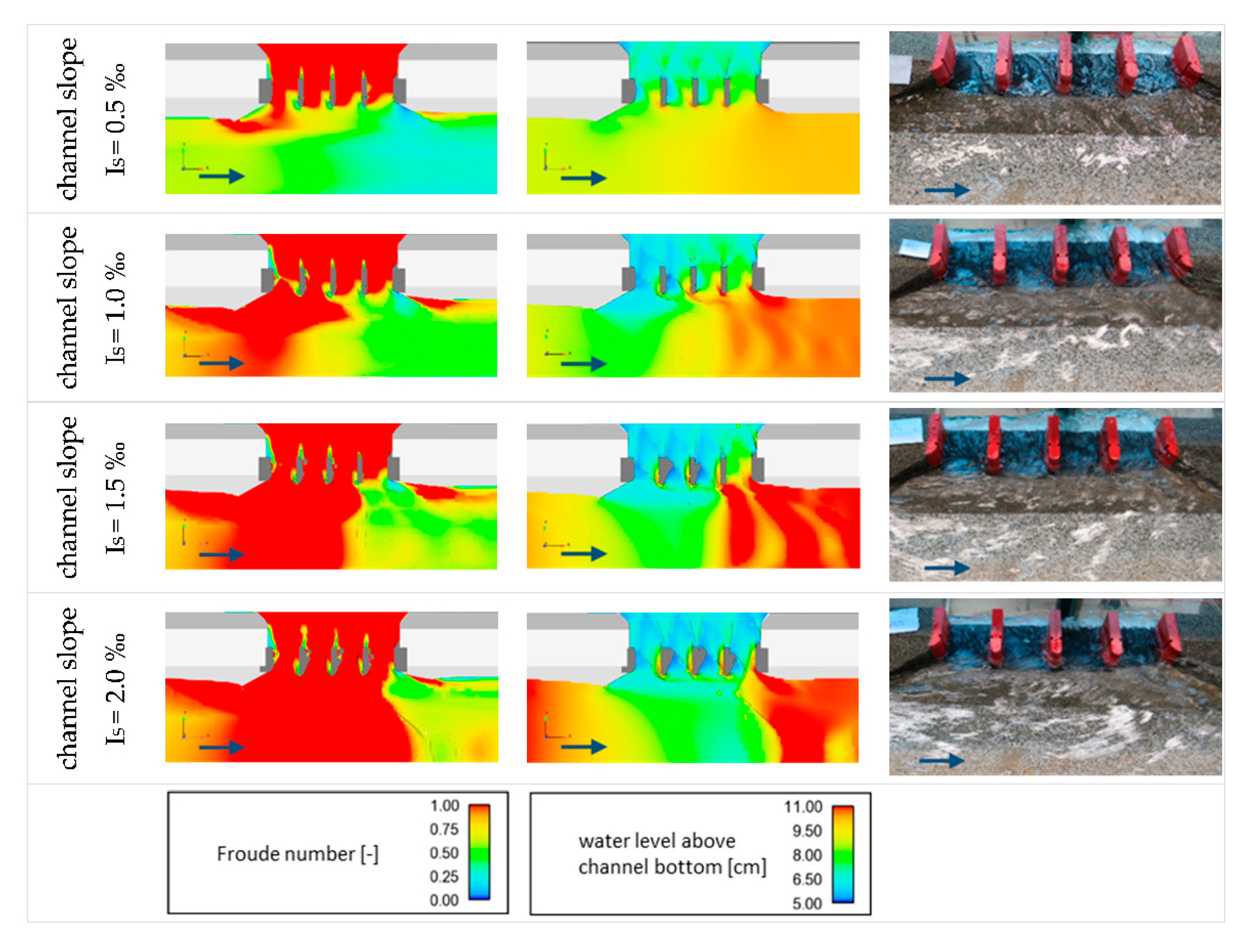
2.3. Validation of the Numerical Simulation Results with a Physical Scale Model

Prior to the parametric study, a validation of numerical simulation results was carried out using a physical model with a scale of 1:50 according to Froude similarity. Due to the limited width of the available glass flume and to avoid surface tension effects in context with the flow behavior over the weir (scale effects), only half of the channel cross-section and a weir with four weir fields were considered in the course of numerical model validation. For the purpose of model validation, the numerical model was adapted accordingly, also accounting for half of the channel cross-section and four weir fields. A comparison of the values in the numerical and in the physical model is shown in

Table 2. Geometric and hydraulic parameters of the physical and the numerical model.

Parameters	Dimensions Numerical Model/Physical Model (1:50)
Channel slope Is	0.5, 1.0, 1.5, 2.0 (‰)
Froude number Fr	0.35, 0.50, 0.65, 0.80 (-)
Channel width B	16.0 (m)/32.0 (cm)
Flow depth h0	3.6 (m)/7.2 (cm)
Flow depth underwater of the weir hd	0.0 (m)/0.0 (cm)
Weir field width b	7.0 (m)/14 (cm)
Weir height w	2.5 (m)/5 (cm)
Number of open weir fields no	0–4 (-)

.

In the experimental flume the channel section was built on a wooden substructure ensuring complete overflow at the weir, avoiding hydraulic influence from water in the weir outflow collection channel. The main channel was constructed of shaped polystyrene blocks, the weir of CNC-milled PVC-elements. A Poncelet weir at the end of a laterally oriented collection channel was used to measure the total discharge leaving via the side weir. An adjustable gate at the downstream end of the channel was used to adapt the boundary conditions according to the particular model configuration. A metal lamella rectifier at the upstream edge of the model ensured uniform flow conditions (Figure 5). Flow depth was evaluated with stationary gauges as well as gauges fixed to a movable gantry. These preliminary investigations included 20 experiments, where the number of weir fields opened (0–4) and the channel slope (0.5–2.0‰) varied. To compare the two modeling approaches, the numerical results first had to be transferred to the model scale, as numerical simulations were carried out on natural scale.

3. Results

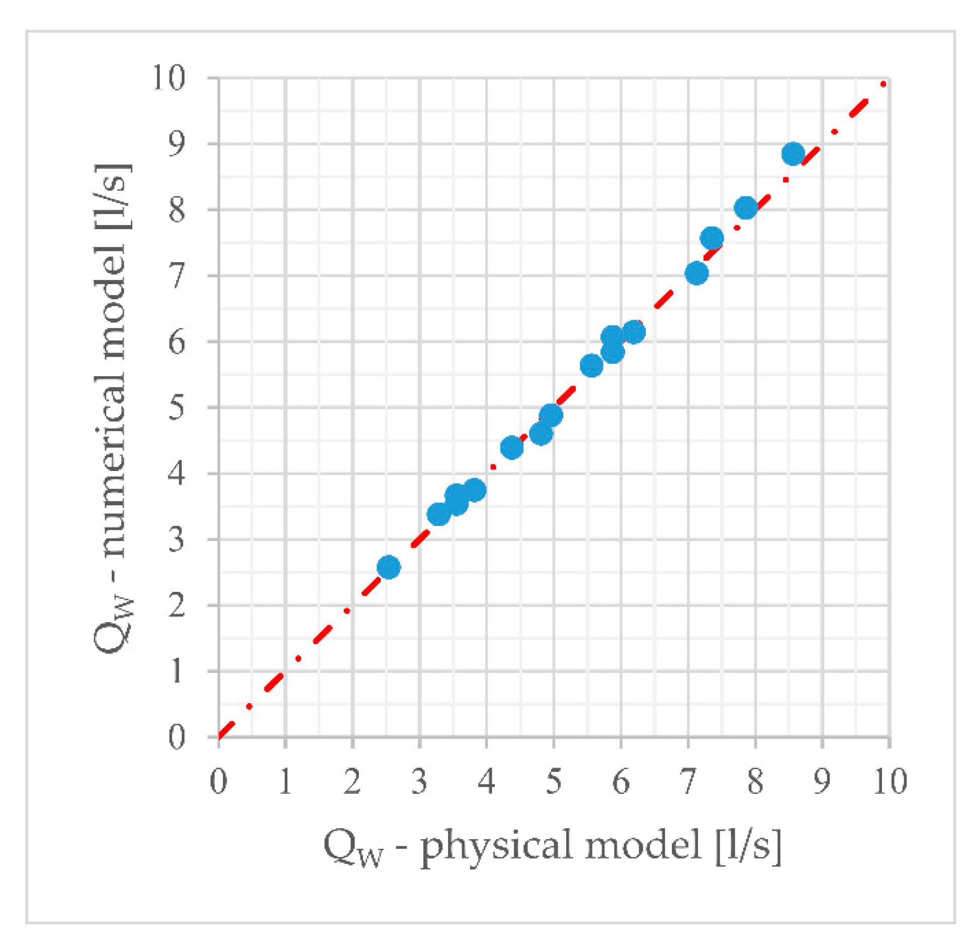
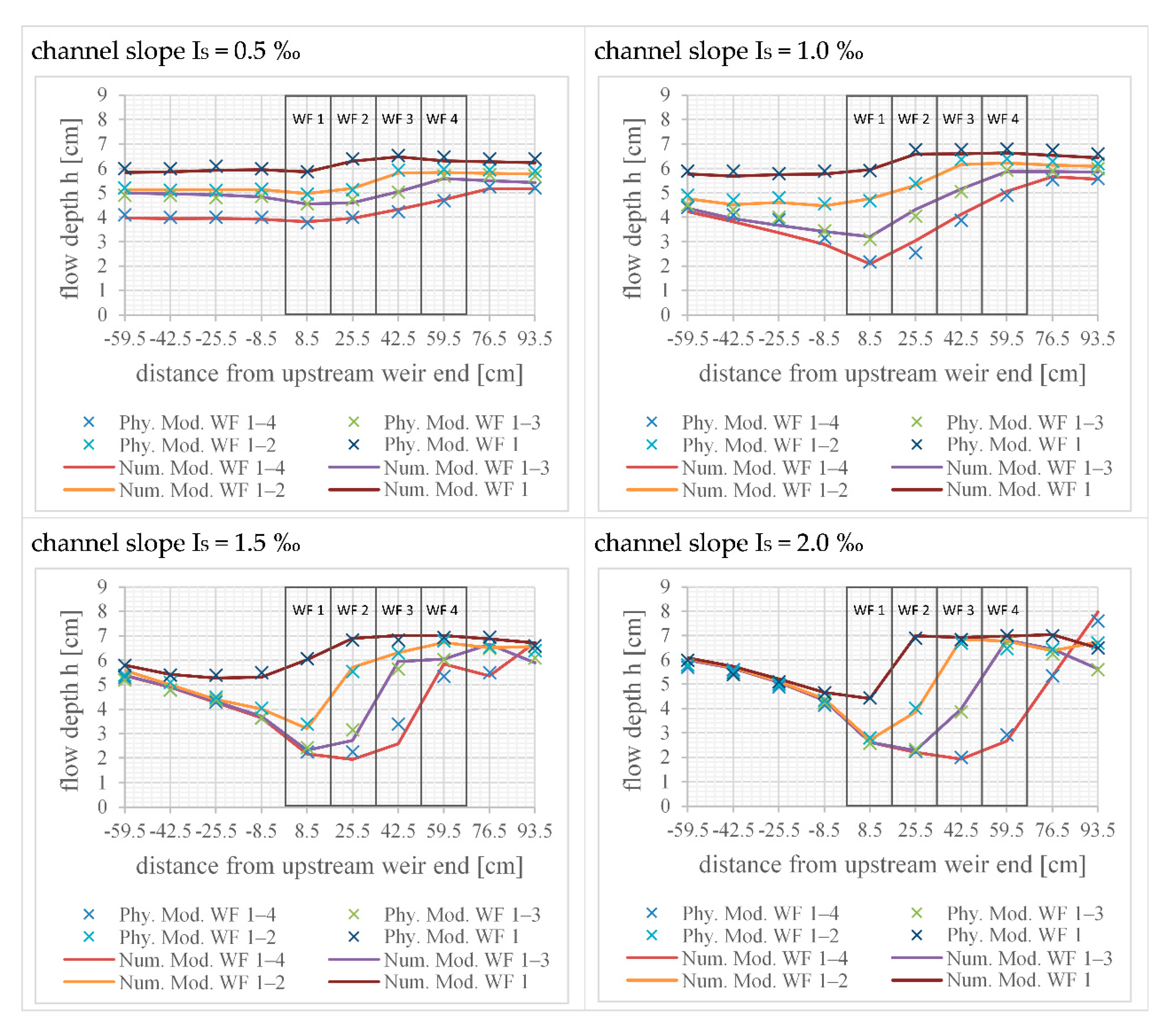
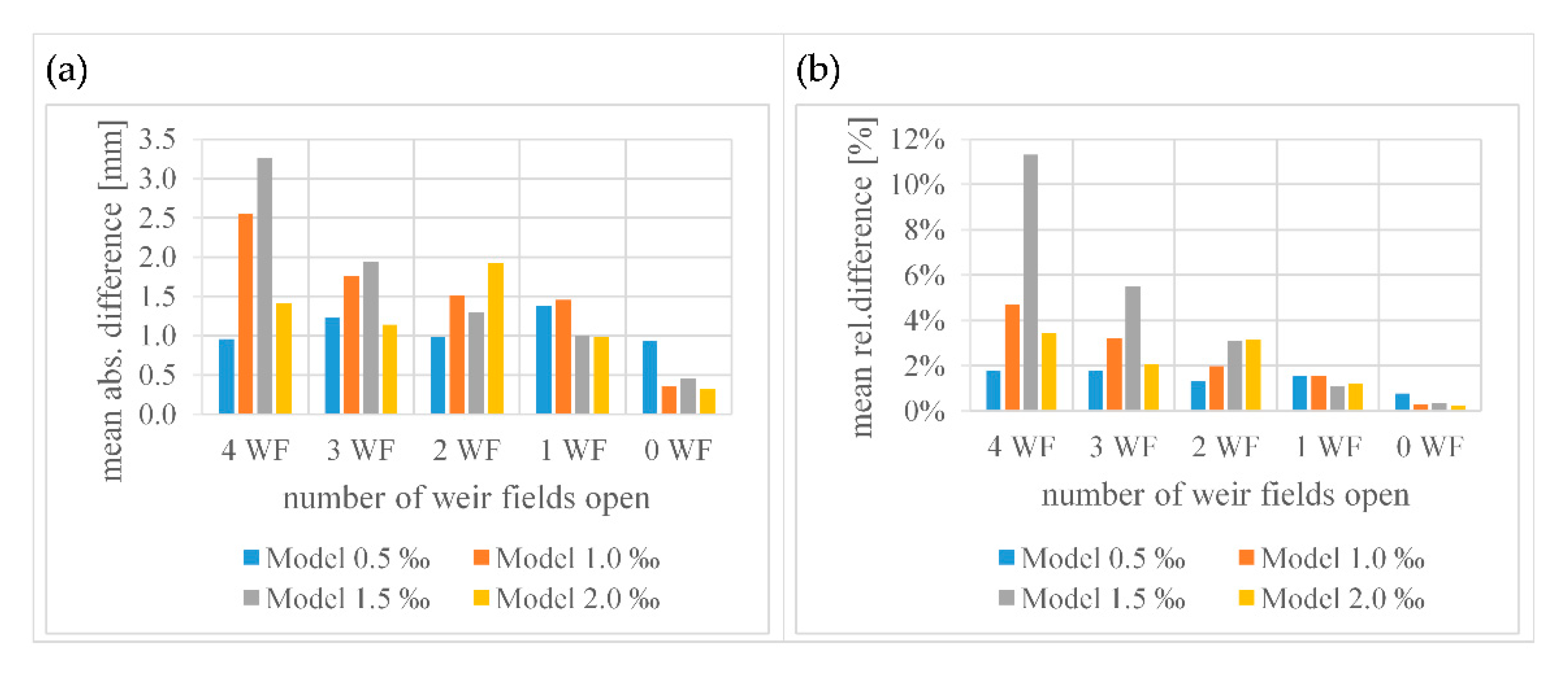
3.1. Comparison of the Numerical and Physical Model Results

To validate the numerical simulations, weir discharges and flow depths at 28 points along 10 cross-sections were recorded in the physical model (Figure 6). The first cross-section was placed 59.5 cm upstream of the upstream end of the weir. The other nine cross-sections were arranged at a distance of 17 cm each, so that sections 5 to 8 encompassed the center of the respective weir fields 1 to 4. The measured values were then compared with the numerical simulation results, which were previously transferred to the model scale. Figure 7 shows the measured weir discharges in the physical model tests versus the results from the numerical simulations, and a very good agreement is observable.

Figure 8 shows profiles of the simulated and measured flow depths along the weir depending on the channel slope and the number of open weir fields. For this representation, the values were averaged along the respective cross-section. Overall, the observed flow depths in the physical model agree very well with those from the numerical simulations.

The evaluation of the absolute and relative differences in Figure 9 underlines this statement. For these diagrams, the difference in flow depth at each point was first determined and then averaged for the respective configuration.

The observed deviations can be explained by the selected measurement method in the physical model and by unsteady flow conditions. The increasing channel slope coupled with discharge reductions and the limited channel width at the upstream end of the weir induced flow state changes from sub- to supercritical. Due to the downstream boundary condition, there was an additional transition along the weir, which resulted in a hydraulic jump. Especially in the model with a channel slope of 1.5‰ in the configuration with all weir fields (4) opened, unsteady waves occurred along the weir and caused uncertainties during the measurement process (Figure 10).

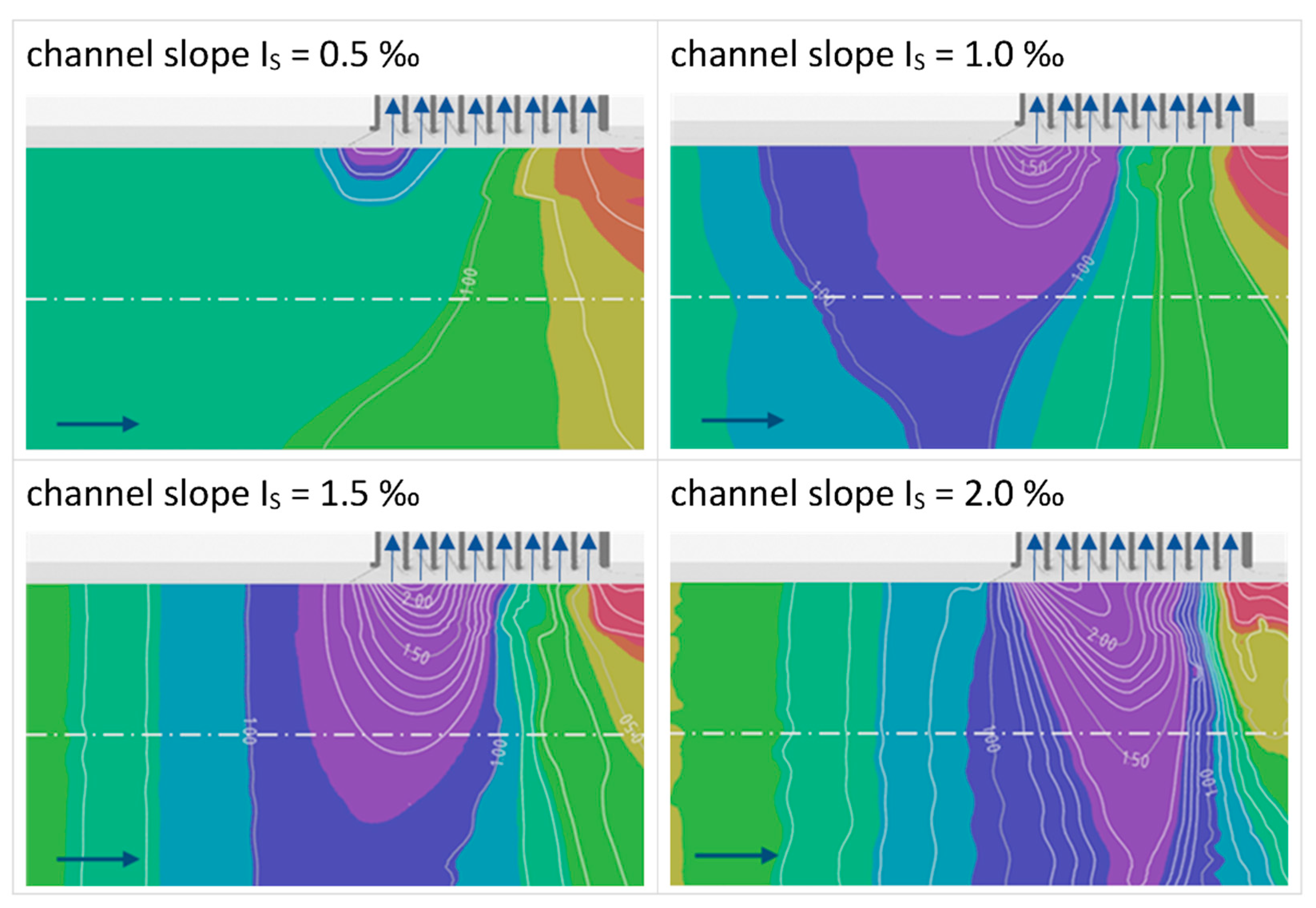
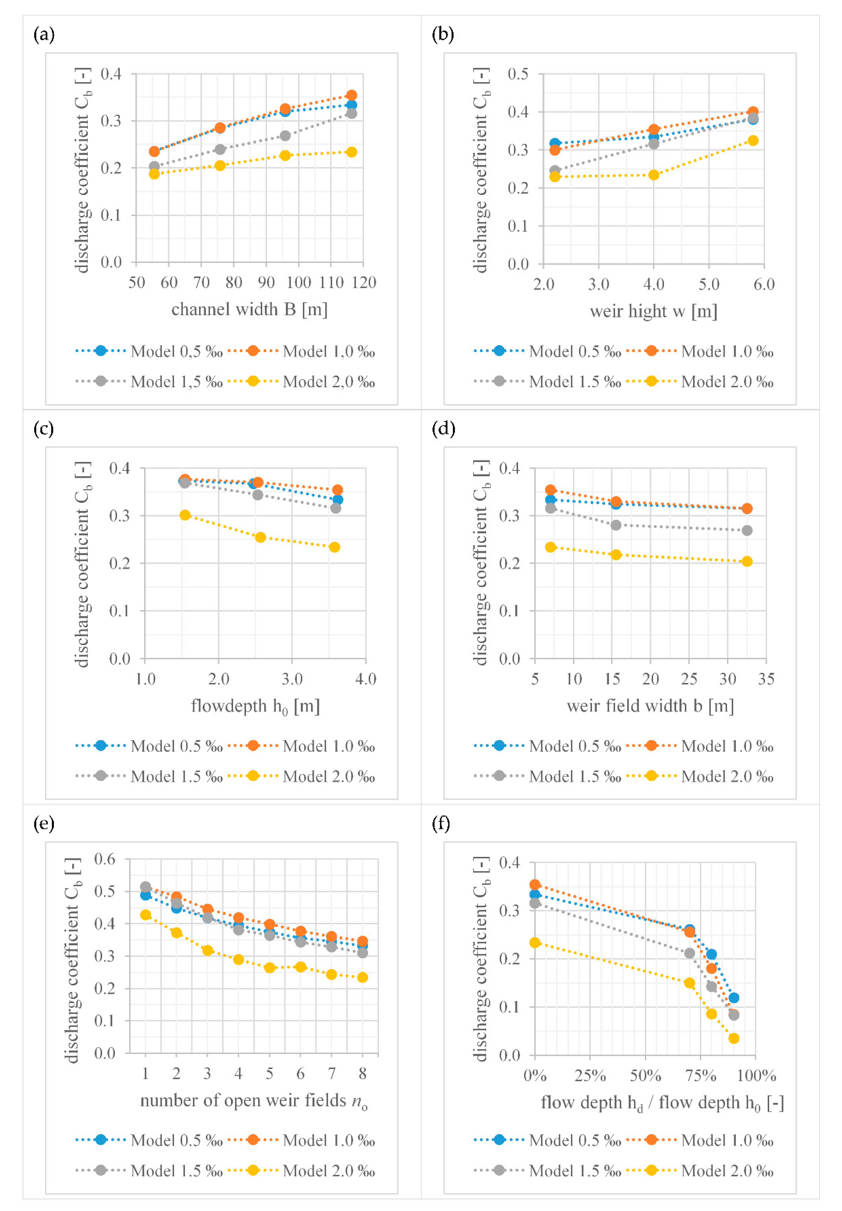
3.2. Influence of Single Parameters on the Discharge Coefficient

The following evaluations aim to describe the influence of the investigated channel and weir parameters on the discharge coefficient (Figure 11). The flow depth h₀ at normal flow conditions upstream of the weir was considered for the determination of the discharge coefficient C_b (Equation (15)), as it not only reflects the actual losses at the weir, but also the impacts of reduced flow depth. As Figure 2 shows, increasing the channel slope yielded significant reductions to the water depth. These circumstances led to reduced weir discharge, even though the models had the same flow depth. The analysis of the discharge coefficient emphasized this effect; models with a slope of 2‰ had the smallest discharge coefficient C_b in almost all variants investigated. Models with 1.0‰ slope showed the largest coefficient C_b, whereas models with 0.5‰ were just slightly lower. As shown in Figure 11a, an extension of the channel width B resulted in an increasing discharge coefficient C_b, whereby models with a channel slope I_S of 0.5 to 1.5‰ were more strongly affected. With the reduction of the channel width B, the impact of the channel slope I_S decreased, which is why the coefficients gradually converge. An increase in weir height relative to the channel bottom also had a positive effect on the discharge coefficient (Figure 11b). As the flow depth above the weir crest declined accordingly, the results showed the opposite behavior. With increasing flow depth h₀, the averaged discharge coefficient C_b decreased (Figure 11c). According to the results in Figure 11d, the coefficient decreases with increasing weir field width b. The arrangement of weir piers and the associated width reduction thus have a positive effect on the discharge capacity. An increasing number of open weir fields leads to a gradual decrease in the discharge coefficient. However, when more weir fields are opened this effect decreases (Figure 11e). The impact of the underwater level shows the typical characteristic as described for example in Aigner and Bollrich [27], for broad-crested weirs. If the flow depth h_d in the underwater rises above 70% in relation to the flow depth h₀, the discharge coefficient is significantly reduced (Figure 11f).

3.3. Regression Analysis

In order to demonstrate the influence of the individual variables on the discharge coefficient, an automated, successive regression analysis was conducted. The variables included in the analysis are in ascending order, depending on their impact on the results. In

Table 3. Successive regression analysis of the averaged discharge coefficient C_b; variables included in the analysis; multiple correlation coefficient R, multiple determination coefficient R², and the standard error.

Variables Included in the Analysis	R	R²	Standard Error	Equation
${\mathrm{C}}_{\mathrm{b}}=\mathrm{f}\left({\left(1-\frac{{\mathrm{h}}_{\mathrm{d}}}{{\mathrm{h}}_0}\right)}^{-0.3}\right)$	0.664	0.414	0.076	(10)
${\mathrm{C}}_{\mathrm{b}}=\mathrm{f}\left(\frac{\mathrm{b}\times n_{\mathrm{o}}}{\mathrm{B}},{\left(1-\frac{{\mathrm{h}}_{\mathrm{d}}}{{\mathrm{h}}_0}\right)}^{-0.3}\right)$	0.866	0.749	0.050	(11)
${\mathrm{C}}_{\mathrm{b}}=\mathrm{f}\left({\mathrm{I}}_{\mathrm{s}}{}^5,\frac{\mathrm{b}\times n_{\mathrm{o}}}{\mathrm{B}},{\left(1-\frac{{\mathrm{h}}_{\mathrm{d}}}{{\mathrm{h}}_0}\right)}^{-0.3}\right)$	0.943	0.888	0.034	(12)
${\mathrm{C}}_{\mathrm{b}}=\mathrm{f}\left({\mathrm{I}}_{\mathrm{s}}{}^5,\frac{{\mathrm{h}}_0}{\mathrm{b}\times {\mathrm{n}}_{\mathrm{o}}},\frac{\mathrm{b}\times n_{\mathrm{o}}}{\mathrm{B}},{\left(1-\frac{{\mathrm{h}}_{\mathrm{d}}}{{\mathrm{h}}_0}\right)}^{-0.3}\right)$	0.954	0.911	0.030	(13)
${\mathrm{C}}_{\mathrm{b}}=\mathrm{f}\left({\mathrm{I}}_{\mathrm{s}}{}^5,\frac{{\mathrm{h}}_0}{\mathrm{b}\times n_{\mathrm{o}}},\frac{\mathrm{b}\times n_{\mathrm{o}}}{\mathrm{B}},\frac{\mathrm{w}}{{\mathrm{h}}_0},{\left(1-\frac{{\mathrm{h}}_{\mathrm{d}}}{{\mathrm{h}}_0}\right)}^{-0.3}\right)$	0.977	0.954	0.022	(14)

the results of this analysis are summarized (Equations (10)–(14)), with the variable $\left(\frac{{\mathrm{h}}_{\mathrm{d}}}{{\mathrm{h}}_0}\right)$ having the highest influence, and the variable $\left(\frac{\mathrm{w}}{{\mathrm{h}}_0}\right)$ with the lowest predicting influence on the coefficient C_b, which varied between 0.01 and 0.53. If the variable $\left(\frac{{\mathrm{h}}_{\mathrm{d}}}{{\mathrm{h}}_0}\right)$ is solely considered in the regression analysis, the estimated value deviates from the simulated coefficient by about 0.076 on average. With an increasing number of variables, this error decreases to a value of 0.022. If all variables are included in the regression analysis, the Equation (15) can be used to determine the discharge coefficient C_b.

$${\mathrm{C}}_{\mathrm{b}}=-0.003\times {\mathrm{I}}_{\mathrm{s}}{}^5+0.253\times \frac{{\mathrm{h}}_0}{\mathrm{b}\times n_{\mathrm{o}}}-0.198\times \frac{\mathrm{b}\times n_{\mathrm{o}}}{\mathrm{B}}+0.036\times \frac{\mathrm{w}}{{\mathrm{h}}_0}-0.228\times {\left(1-\frac{{\mathrm{h}}_{\mathrm{d}}}{{\mathrm{h}}_0}\right)}^{-0.3}+0.603$$

(15)

Figure 12 demonstrates the correlation between the simulated discharge coefficients, which were used as the dependent variables in the regression analysis, and the values calculated based on the obtained regression equation (Equation (15)). In the regression analysis, a multiple correlation coefficient of 97.7% and a multiple determination coefficient of 95.4% were obtained. The significance was found to be clearly below the specified significance level of 1%.

4. Conclusions

The conducted 3D numerical simulations represent an additional contribution to analyze the discharge behavior of side weirs with several weir fields in an open channel. Widely used approaches by De Marchi [2], Schmidt [19] and Dominguez [20] are subject to limitations in their application due to the geometric specifications and the way they are derived. In reality, the given spatial variability of flow depths when weirs are open and water is diverted makes it impossible to specify a representative location used for the calculation of the weir discharge. To overcome this drawback a novel approach was developed, where derived equations refer to the water surface level that corresponds to the normal flow depth in the main channel, located closely upstream of the water level surface drawdown. In the case of prismatic channels, this corresponds to the normal flow depth at the weir when the weir fields are closed. The numerical model, used to simulate different weir and channel configurations, was validated with results from a physical model test. Overall, this comparison shows good agreement and supports the applied numerical model assumptions. In the course of a parametric study, the losses at the structure as well as the spatial reduction in water surface caused by the opening of the individual weir fields could be determined and their influence on the discharge behavior was depicted. Through a regression analysis based on the numerical simulation results, a formula for the estimation of the discharge coefficient was derived (Equation (15)). This formula can be used for the dimensioning of new weirs, while also proving applicable to the operation of existing side weirs with several weir fields, whose local conditions and structural design correspond to the characteristics of the carried out parametric study (Table 1). However, especially in natural river sections with changing geometric and hydraulic conditions, a critical evaluation of the results is required.

References

1. May, R.W.P.; Bromwich, B.C.; Gasowski, Y.; Rickard, C.E. Hydraulic Design of Side Weirs, 1st ed.; Thomas Telford: London, UK, 2003; ISBN 978-0-7277-3167-8. [Google Scholar]
2. De Marchi, G. Saggio di teoria sul funzionamento deglistramazzi laterali. L’Energia Elettr. 1934, 11, 849–854. [Google Scholar]
3. Borghei, S.M.; Jalili, M.R.; Ghodsian, M. Discharge Coefficient for Sharp-Crested Side Weir in Subcritical Flow. J. Hydraul. Eng. 1999, 125, 1051–1056. [Google Scholar] [CrossRef]
4. Cheong, H. Discharge Coefficient of Lateral Diversion from Trapezoidal Channel. J. Irrig. Drain. Eng. 1991, 117, 461–475. [Google Scholar] [CrossRef]
5. Hager, W.H. Lateral Outflow Over Side Weirs. J. Hydraul. Eng. 1987, 113, 491–504. [Google Scholar] [CrossRef] [Green Version]
6. Ranga Raju, K.G.; Gupta, S.K.; Prasad, B. Side Weir in Rectangular Channel. J. Hydraul. Div. 1979, 105, 547–554. [Google Scholar] [CrossRef]
7. Singh, R.; Manivannan, D.; Satyanarayana, T. Discharge Coefficient of Rectangular Side Weirs. J. Irrig. Drain. Eng. 1994, 120, 814–819. [Google Scholar] [CrossRef]
8. Subramanya, K.; Awasthy, S.C. Spatially Varied Flow over Side-Weirs. J. Hydraul. Div. 1972, 98, 1–10. [Google Scholar] [CrossRef]
9. Di Bacco, M.; Scorzini, A.R. Are We Correctly Using Discharge Coefficients for Side Weirs? Insights from a Numerical Investigation. Water 2019, 11, 2585. [Google Scholar] [CrossRef] [Green Version]
10. El-Khashab, A.; Smith, K.V. Experimental Investigation of Flow over Side Weirs. J. Hydraul. Div. 1976, 102, 1255–1268. [Google Scholar] [CrossRef]
11. Emiroglu, M.E.; Ikinciogullari, E. Determination of Discharge Capacity of Rectangular Side Weirs Using Schmidt Approach. Flow Meas. Instrum. 2016, 50, 158–168. [Google Scholar] [CrossRef]
12. Namaee, M.R.; Jalaledini, M.S.; Habibi, M.; Yazdi, S.R.S.; Azar, M.G. Discharge Coefficient of a Broad Crested Side Weir in an Earthen Channel. Water Sci. Technol. Water Supply 2013, 13, 166–177. [Google Scholar] [CrossRef]
13. Říha, J.; Zachoval, Z. Flow characteristics at trapezoidal broad-crested side weir. J. Hydrol. Hydromech. 2015, 63, 164–171. [Google Scholar] [CrossRef] [Green Version]
14. Uyumaz, A.; Muslu, Y. Flow Over Side Weirs in Circular Channels. J. Hydraul. Eng. 1985, 111, 144–160. [Google Scholar] [CrossRef]
15. Castro-Orgaz, O.; Hager, W. Subcritical Side-Weir Flow at High Lateral Discharge. J. Hydraul. Eng. 2012, 138, 777–787. [Google Scholar] [CrossRef] [Green Version]
16. Crispino, G.; Cozzolino, L.; Della Morte, R.; Gisonni, C. Supercritical Low-Crested Bilateral Weirs: Hydraulics and Design Procedure. J. Appl. Water Eng. Res. 2015, 3, 35–42. [Google Scholar] [CrossRef]
17. Chow, V.T. Open-Channel Hydraulics; McGraw-Hill: New York, NY, USA, 1959. [Google Scholar]
18. Poleni, G. De Motu Aquae Mixto Libri Duo; Kessinger Publishing: Padova, Italy, 1717. [Google Scholar]
19. Schmidt, M. Gerinnehydraulik; Bauverlag GmbH: Wiesbaden, Germany, 1957. [Google Scholar]
20. Dominguez, F.J. Hidraulica; Editorial Universitaria: Santiago, Chile, 1999. [Google Scholar]
21. Shariq, A.; Hussain, A.; Ansari, M.A. Lateral Flow through the Sharp Crested Side Rectangular Weirs in Open Channels. Flow Meas. Instrum. 2018, 59, 8–17. [Google Scholar] [CrossRef]
22. Martin, H.; Pohl, R. Technische Hydromechanik 4—Hydraulische und numerische Modelle, 3rd ed.; Beuth Verlag GmbH: Berlin, Germany, 2015. [Google Scholar]
23. SPSS IBM. SPSS Statistics for Windows; Version 24.0; IBM Corp.: Armonk, NY, USA, 2016. [Google Scholar]
24. Flow Science, Inc. FLOW-3D® Solver; Version 11.2; Flow Science, Inc.: Santa Fe, NM, USA, 2017. [Google Scholar]
25. Hirt, C.W.; Nichols, B.D. Volume of Fluid (VOF) Method for the Dynamics of Free Boundaries. J. Comput. Phys. 1981, 39, 201–225. [Google Scholar] [CrossRef]
26. Launder, B.E.; Spalding, D.B. The Numerical Computation of Turbulent Flows. Comput. Methods Appl. Mech. Eng. 1974, 3, 269–289. [Google Scholar] [CrossRef]
27. Aigner, D.; Bollrich, G. Handbuch der Hydraulik für Wasserbau und Wasserwirtschaft, 1st ed.; Beuth Verlag GmbH Berlin: Zurich, Vienna, 2015. [Google Scholar]
Figure 1. Water surface (represented by flow depth y) and energy line (parameter E) in a one-dimensional approach at a side weir at subcritical flow conditions (modified after De Marchi [2]); flow direction from left to right.
Water 13 01717 g001
Figure 2. Spatially distributed drawdown of the water surface in the channels (m) due to water diversion through the side weir with eight open weir fields (blue arrows); channel slope IS ranges between 0.5 and 2.0‰; the illustrated contour lines reflect the reduction of flow depth in meters compared to the undisturbed normal flow depth; the dash-dot line represents the main channel axis; the main flow direction is from left to right.
Water 13 01717 g002
Figure 3. Schematic sketch of the side weir with eight weir fields—cross-section through the main channel and side weir (a) and plan view (b).
Water 13 01717 g003
Figure 4. Arrangement and dimensions of the Cartesian mesh blocks (border lines in cyan blue), position of the defined monitoring points.
Water 13 01717 g004
Figure 5. Physical scale model of the side weir with four weir fields in an experimental flume; rectifier at the upstream edge of the model (a); height-adjustable gate at the downstream edge of the model (b); channel collecting side weir discharge with a Poncelet weir (c).
Water 13 01717 g005
Figure 6. Arrangement of the 28 monitoring points at 10 cross-sections along the side weir; flow direction from left to right.
Water 13 01717 g006
Figure 7. Comparison of weir discharges in the physical and numerical model.
Water 13 01717 g007
Figure 8. Profiles of the flow depths h above the weir crest determined in the numerical and in the physical model along the weir depending on the number of weir fields opened for channel slopes of 0.5–2.0‰ (including position of weir fields 1–4); flow direction from left to right.
Water 13 01717 g008
Figure 9. Mean absolute (a) and relative (b) difference of the flow depths h resulting from the numerical and the physical model.
Water 13 01717 g009
Figure 10. Plots of the Froude number and the flow depths in the numerical model as well as photos of the physical model in the configuration with all weir fields (4) opened for channel slopes of 0.5–2.0‰; flow direction from left to right.
Water 13 01717 g010
Figure 11. Influence of the analyzed weir and channel parameters on the discharge coefficient Cb; channel width B (a); weir height w (b); flow depth h0 (c); weir field width b (d); number of open weir fields no (e); ratio of underwater flow depth hd and flow depth h0 at normal flow conditions closely upstream of the weir (f).
Water 13 01717 g011
Figure 12. Comparison of the simulated and calculated discharge coefficients Cb.
Water 13 01717 g012