Magnolia and Viburnum Plant Factors at Different Growing Seasons and Allowed Depletion Levels in a Monsoonal Climate

Abstract

We investigated seasonal water use, growth and acceptable root-zone water depletion levels to develop tools for the more precise irrigation of two Southeast U.S. landscape species in a monsoonal climate—Magnolia grandiflora and Viburnum odoratissimum. The study was conducted under a rainout shelter consisting of two concurrent studies. One, weighing lysimeter readings of quantified water use (ET_A) at different levels of irrigation frequency that dried the root zone to different allowable depletion levels (ADL). Two, planting the same species and sizes inground and irrigating them to the same ADLs to assess the effect of root-zone water depletion on growth. The projected crown area (PCA) and crown volume were concurrently measured every three weeks in both studies as well as reference evapotranspiration (ETo). Plant factor values were calculated from the ratio of ET_A (normalized to depth units by PCA) to ETo. The two species had different tolerances for irrigation frequency depending on the season: peak magnolia canopy growth was mid-spring to mid-summer, while peak viburnum canopy growth was summer. Canopy growth for both species was most sensitive to greater ADL-water stress during the peak growth stages of both species. For urban landscape irrigation, these data suggest that 60–75% of available water in magnolia and viburnum root zones can be depleted before irrigation and that they can be irrigated at a plant factor (PF) value of 0.6 of ETo. For landscape situations with high expectations, such as during establishment and especially during peak growth, a wetter water budget that minimizes water stress would be more appropriate: 30–45% ADL and PF values of 0.7–0.8. The results of this study are aimed at water managers and landscape architects and designers in a humid climate who need to account for water demand in planning scenarios.

1. Introduction

Often the most important component of urban landscapes, woody plants and trees, typically require irrigation to sustain their health and value. Climate change and drought are forcing landscape managers to be more efficient in conserving water while maintaining woody plant health. This efficiency is achieved with a water budget: irrigating woody plants with just enough at the right time before they become water stressed [1]. A water budget requires reasonable estimates of plant water demand and root-zone depletable water levels to determine when and how much to irrigate.

Adapted from agriculture, the accepted approach for estimating plant water demand is to use an empirically derived correction factor, Plant Factor (PF) (i.e., actual water use divided by reference evapotranspiration (ETo) which is equivalent to Kc in agriculture), to adjust downward the local ETo for a given plant type [1]. However, in general there are limited landscape plant water-use studies on which to base a tool for estimating water demand. Information for humid, high-rainfall climates is particularly limited, even more so for monsoonal, subtropical climates that have both dry and high-rainfall seasons. Furthermore, extant studies have focused largely on trees in temperate-arid to semi-arid climates [2] rather than on shrubs [3,4,5,6,7,8]. Finally, these water-use studies are rarely paired with an investigation into the amount of root-zone water that can be safely depleted before irrigation is required, an important piece of irrigation information in any climate that determines how much a plant can safely mine root-zone water without stress.

The objective of this study was to determine PF values and acceptable root-zone water depletion levels (water stress) for two common woody ornamentals in southeastern U.S. landscapes––the southern magnolia (Magnolia grandiflora) and sweet viburnum (Viburnum odoratissimum––in a dry spring/high summer rainfall monsoonal climate.

2. Materials and Methods

This research consisted of two concurrent experiments for each species. The first used hanging weighing lysimeters to quantify water use of a tree and a shrub species irrigated at different allowed depletion levels (ADLs) to understand how PF values vary with ADL water stress. A complementary study used established inground plants that were irrigated at the same ADL rates but more precisely monitored to assess the minimum ADL that achieved acceptable growth with the least amount of water in a setting more representative of a landscape. Experiments were conducted in an open-side, clear, double polyethylene-covered rainout shelter of 300 m² at the University of Florida Mid-Florida Research and Education Center (MREC) near Orlando during the summer 2008 and spring 2009. Plant materials consisted of Southern magnolia (Magnolia grandiflora L. “D.D. Blanchard”), and sweet viburnum (Viburnum odoratissimum Ker Gawl). These two species were chosen because both are evergreen and commonly used in commercial and residential landscapes throughout the southeastern United States. The lysimeter and inground studies were repeated during typical dry spring conditions and again during high rainfall summer conditions during central Florida’s monsoons.

2.1. Plant Material and ADL Treatments

Southern magnolia in #7 (26.5 L) containers and sweet viburnum in #3 (11.4 L) containers were obtained from a local nursery. To establish plants, the southern magnolias were transplanted in #15 (57 L) containers and the sweet viburnums were transplanted into #7 (26.5 L) containers. The substrate used for transplanting was a standard 60% composted pine bark, 30% NuPeat and 10% sand mixture amended with micronutrients and dolomite, and fertilized with 54 g of Osmocote 14–14–14 (Scotts Co., Marysville, OH, USA) per plant. Transplanted plants were then placed in a full-sun production area for additional growth and irrigated to field capacity several times a day using two spray stakes (Roberts Irrigation), and allowed to grow for two weeks. Plants were fertilized, irrigated and allowed to grow until installed in lysimeters in the rainout shelter.

The rainout shelter was separated into southern magnolia and sweet viburnum planting areas, each with four replicate rows. Southern magnolia replications consisted of four trees installed inground, alternating with four trees in lysimeters one meter apart. There were 16 southern magnolias planted both in lysimeters and inground. Each sweet viburnum row had four lysimeter plants, with two near the ends of the bay and two in the middle, creating three uniform planting spaces. In each planting space between lysimeters, three sweet viburnums were planted 0.6 m apart inground. There were 16 sweet viburnums in lysimeters, and 12 groups of sweet viburnums planted inground. Only the growth of sweet viburnums in the middle of each group were measured during the study.

Treatments for both species consisted of the depletion of the percentage of plant available water the before a container or soil was irrigated back to 100% capacity. The higher the allowed depletion level (ADL), the higher the drought stress level, resulting in less irrigation frequency and less water applied in total. Southern magnolia in both lysimeters and inground were randomly assigned into four treatments, 30, 45, 60, and 75% ADL, with four replicates each, resulting in 70, 55, 40, and 25 plant available water remaining in a root ball before irrigation was electronically triggered the following evening. The 16 sweet viburnum plants in lysimeters were randomly assigned to four irrigation treatments, 10, 30, 50, and 70 ADL, with four replicates each. The 12 groups of sweet viburnums were randomly assigned the same ADL levels, with three single-plant replicates each flanked by two border plants.

2.2. Hanging Lysimeter Setup and Data Collection

To quantify water use and develop PF values, the hanging lysimeter methodology of Beeson was followed [9]. Plants in 0.62 m diameter lysimeter pots were suspended from a metal tripod within inground dry wells made from corrugated plastic drain tile at lengths of 45 to 50 cm. Suspending plants in inground wells limited the heat loading of plastic containers and prevented wind instability. A load cell (45.36 kg capacity) was attached to the inside top of each tripod from which the study plants were suspended inside a metal strap basket. The suspended baskets containing the study plants in 23 L (C2800, Nursery Supply) were adjusted such that container top edge were even with tops of the wells. Wires extended from each load cell to two multiplexers (AM-32 and AM16-32, Campbell Scientific, Logan UT) connected to a datalogger (CR10X, Campbell Scientific, Logan UT) that recorded weight changes due to volumetric plant water use from the plant-container system in 24 h periods. Volumetric water-use totals registered as daily weight changes were translated into irrigation run time by a datalogger program to replace water lost to the desired depletion levels. The datalogger was wired to two relay modules (SDM CD-16ACDC, Campbell Scientific, Logan, UT, USA), each controlling an electric solenoid valve for each lysimeter. The solenoid then was opened by the datalogger program to supply water through 2.54 cm black polyethylene tubing to each suspended container, from which two 0.63 mm micro-irrigation lines were installed that were terminated with spray stakes (Blue pot stakes, 39.4 L/h Maxijet Inc., Dundee, FL, USA). Each lysimeter was calibrated in place with precision weights to 22.7 kg to create a 7-point linear fit.

To apply the irrigation treatments, we first determined plant-available water in the substrate. Initially each container was irrigated to 100% container capacity, allowed to drain, and then weighed. Water loss by transpiration and surface evaporation (actual evapotranspiration) was then allowed to proceed until each plant was visibly water stressed (i.e., wilting) by late morning. The differences in lysimeter mass between the night after water stress and at 100% capacity were calculated to be the quantity of plant available water within each root ball, from which the ADL values applied.

Plants of both species were irrigated daily at midnight to 100% container capacity using a micro-irrigation system for the first two weeks. Then, irrigation frequency was gradually reduced to bring each lysimeter irrigation level to the appropriate ADL level. Daily plant water use was calculated at midnight each day for each lysimeter and values were summed until the cumulative ET_A exceeded the amount of allowed depletion for each plant depending on ADL treatments. When this occurred, a container was irrigated. Irrigation was applied in three different volumes at midnight, 1:00, and 2:00 h with the total applied volume equaling 1.2 times the cumulative ET_A. The extra 20% was to account for increases in plant mass, which offset transpiration water loss and imperfect irrigation coverage and was accounted for by the beginning of the daily data collection when container weight was in a steady state. During the data collection period, the canopy variables of the widest width, width perpendicular to widest width, and canopy height were recorded every three weeks.

2.3. Inground Study Setup and Data Collection

To assess growth for the same ADL irrigation treatments, the same species and sizes were installed under a rainout shelter in native sandy soil (Apopka association: loamy, siliceous, subactive, hyperthermic Grossarenic Paleudult). For the purpose of applying irrigation treatments, we measured volumetric root-zone water content (Ѳv) with EC-5 probes (Decagon Devices, Pullman, WA, USA) installed in both southern magnolia and sweet viburnum inground studies. Probes were installed slightly off-vertical, with probe sensors measuring volumetric water content within the 10 to 15 cm soil layer below the soil surface. One probe was installed for each inground southern magnolia, but for the sweet viburnum, two probes were installed in each group halfway between the center plant and the two border plants.

All EC-5 soil moisture probes were calibrated with the existing soil before each experiment in 2008 and 2009 by determining field capacity and the wilting point. We measured the field capacity at each sensor location by saturating the soil at midnight, then determining the percent volumetric water content at the point of deflection later that morning. The Ѳv declined linearly through most of the night after irrigation, but in the early morning the decline stopped or slowed before sunrise, at which point a measurement was taken to represent field capacity. Available water and ADLs were determined from dehydration curves developed from the mean of six samples using a pressure-plate system (Soil Moisture Equipment Inc., Goleta, CA, USA). Field capacity was the amount of water (Ѳv) after saturating the soil and 24 h of drainage; and wilting point was Ѳv assumed to be at −1.5 MPa. Allowed depletion thresholds that triggered irrigation were calculated as follows:

Ѳv _{Irrigation threshold} = Ѳv _{Field capacity} − (Ѳv _{Field capacity} − Ѳv _{−15 bar}) × ADL as decimal

(1)

For sweet viburnum, irrigation was applied with two 360° inverted cone nozzles (Maxijet, Dundee, FL, USA) per study plant on a 30 cm stake in the middle on either side of the center plant. Two 180° nozzles (Maxijet, Dundee, FL, USA) with half the output were placed on 30 cm stakes on the outside of either end of the planting. For each southern magnolia, two 180° nozzles (Maxijet, Dundee, FL, USA) with half the output used for sweet viburnum were placed on similar 30 cm stakes on either side of a plant. Irrigation frequencies were reduced gradually over two weeks such that plants obtained their assigned ADL at the beginning of data collection. During this period, irrigation was controlled by the results of the soil moisture sensors and the datalogger. Again, growth measurements of height, widest width, and width perpendicular to the widest width were recorded on the center plant of each group of sweet viburnum and on each southern magnolia inground every three weeks.

During the experiment, irrigation occurred at 01:00 h only when % volumetric water content (Ѳv) of both sensors per replication were below their respective threshold levels. Irrigation continued until the Ѳv of both sensors was 25% or greater. The Ѳv at field capacity generally ranged between 15 and 20%. The 25% volumetric water content (VWC) was set so that irrigation would percolate below sensors to the roots below. After treatments were designated, irrigation frequency was gradually decreased by increasing the ADL for all levels over three to five days.

2.4. Weather

In March 2008, a weather station was installed in the middle of the rainout shelter. The station consisted of a CR10X data logger (Campbell Scientific, Logan, UT, USA) to which a temperature/relative humidity sensor (CS-215, Campbell Scientific, Logan, UT, USA), a pyranometer (LI-200, LiCor Inc., Lincoln, NB, USA), a wind sensor (014, Met-One, Bend, OR, USA), and a quantum sensor (model LI-190R) to measure photosynthetically active radiation (PAR) were attached. The pyranometer and quantum sensor were mounted 3.35 m above ground level to limit shading by the rain shelter. The temperature/relative humidity sensor and anemometer were mounted 2 m above ground level. Daily reference evapotranspiration (ETo) was calculated using Campbell Scientific Application Note 4D. It calculated the full American Society of Civil Engineers (ASCE) Penman–Monteith equation with resistances [10].

2.5. Data Analysis

For the lysimeter study, daily water use in volume units was normalized to depth units by dividing by PCA for a given time period to derive water use in depth units (ET_A). Again, daily water was obtained from the datalogger calculations used in applying ADL treatments, and time-period PCA was estimated by nesting the average of the measured PCA taken every three weeks. For example, PCA was measured on the first and fifteenth day of the month and averaged to represent the PCA of the seventh day of each period. Then the first and seventh day PCA measurements were averaged to estimate the 4th day PCA and so forth to arrive at a derived daily PCA. This iterative process was used to calculate a 10-day rolling ET_A average of the previous 10 days’ daily ET_A rate to arrive at ET_A in mm day⁻¹. The PF calculations for the summer of 2008 were based on water use between 1 April and 4 August 2008 for both sweet viburnum and southern magnolia. Spring 2009 calculations were based on water use between 17 December 2008 and 19 April 2009 for sweet viburnum only because it is an evergreen and exhibits continuous growth flushes. The southern magnolia, while also evergreen, has a bud break in Central Florida in mid-April followed by a vigorous growth period, so we extended spring data collection for southern magnolias from 15 March to 18 June to encompass peak growth. Each time period was based on the first day of collecting PCA measurements. The averaged PCA for each time period was used for PF calculations for each plant. We calculated plant factors by taking daily ET_A in depth units and dividing them by daily ETo for a given time period.

The experiment was designed as a randomized complete block design. Pairwise comparisons for growth were completed using the R software (version R×64.3.5.2) to run one-way ANOVA test and an LSD test with a significance level of 0.05, and pairwise comparisons for 2008 and 2009 PF were completed using a paired t-test.

3. Results

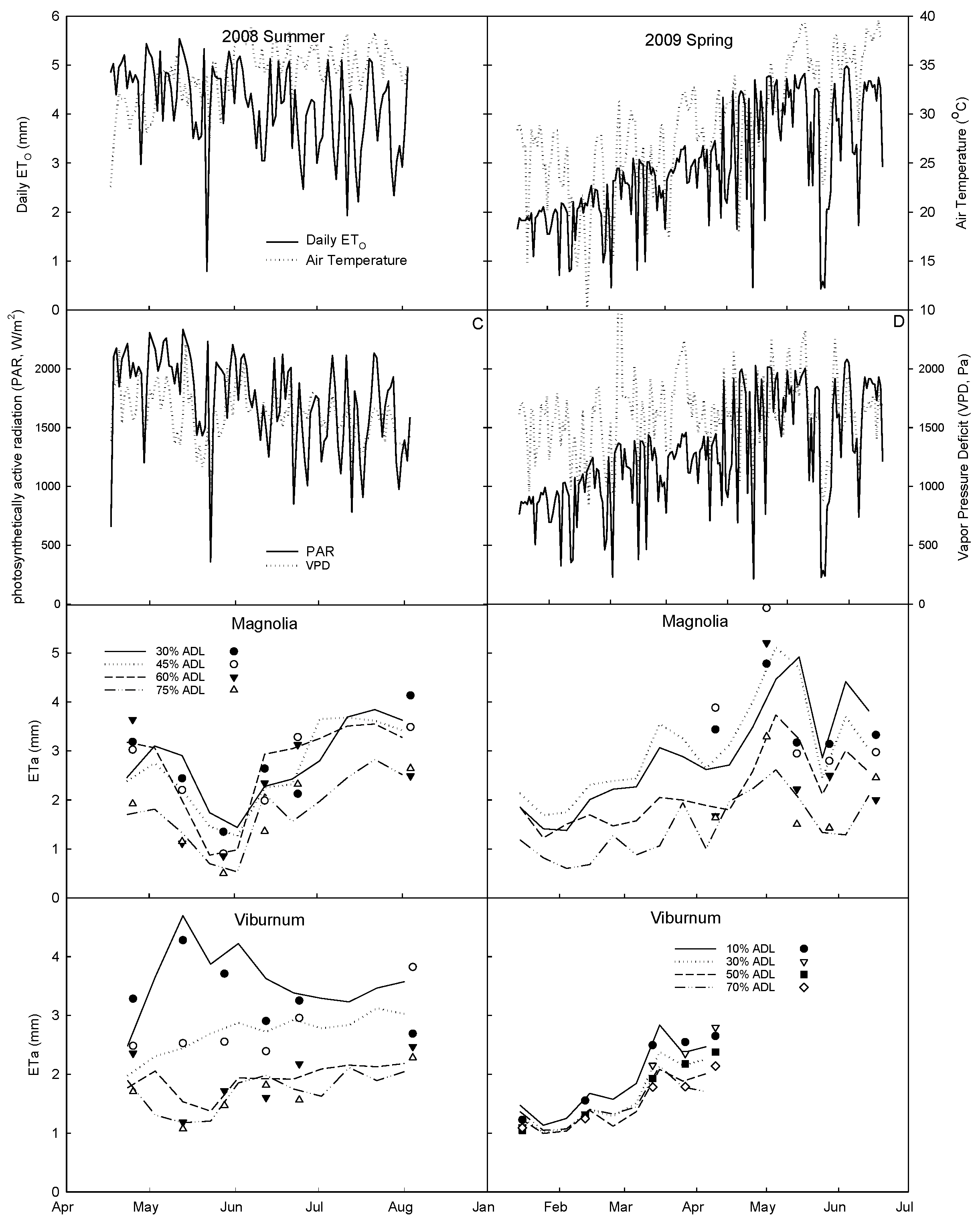
Weather during the two study periods was characteristic of the monsoonal seasons in central Florida independent of rainfall within the rainfall shelter (Figure 1A–D). The winter–spring dry season showed a characteristic steady increase in air temperature (Ta) and solar radiation that pushed the ET_O from about 2.5 in January to 5 mm/day by late May due to higher sun angles, longer days and warmer temperatures (Figure 1A–D). The weather was more variable due to cloudiness and storms during the June–October summer wet season. This meant that while temperatures were higher than in spring, vapor pressure deficit (VPD) was overall lower and PAR fluctuated wildly from day to day, as did ET_O, ranging from 3.8 to 5 mm per day (Figure 1A–D). In a humid climate, such as central Florida, incoming solar radiation is the primary driver of ET_O [11,12], unlike arid climates where the VPD is the main driver [2]. Air was the driest in spring, as the VPD peaked at 2.5 kPa in March–May at the end of the dry season, staying below 2 kPa during the wet season, minimally contributing to evapotranspiration. By contrast, the VPD can range up to 5 kPa or more in arid–semi-arid climates and drive plant water use more than does radiation [2]. We did note that the rainout shelter ET_O was approximately 20% less than that calculated from a nearby (0.5 km) full-sun weather station due to some attenuation of incoming solar radiation (data not shown). However, we assumed that plant water use under the rainout shelter would be affected the same as the ETo under the shelter. Since PF values here were based on the 20% lower ET_O inside the rainout shelter, we believed the PF values were applicable to full-sun conditions.

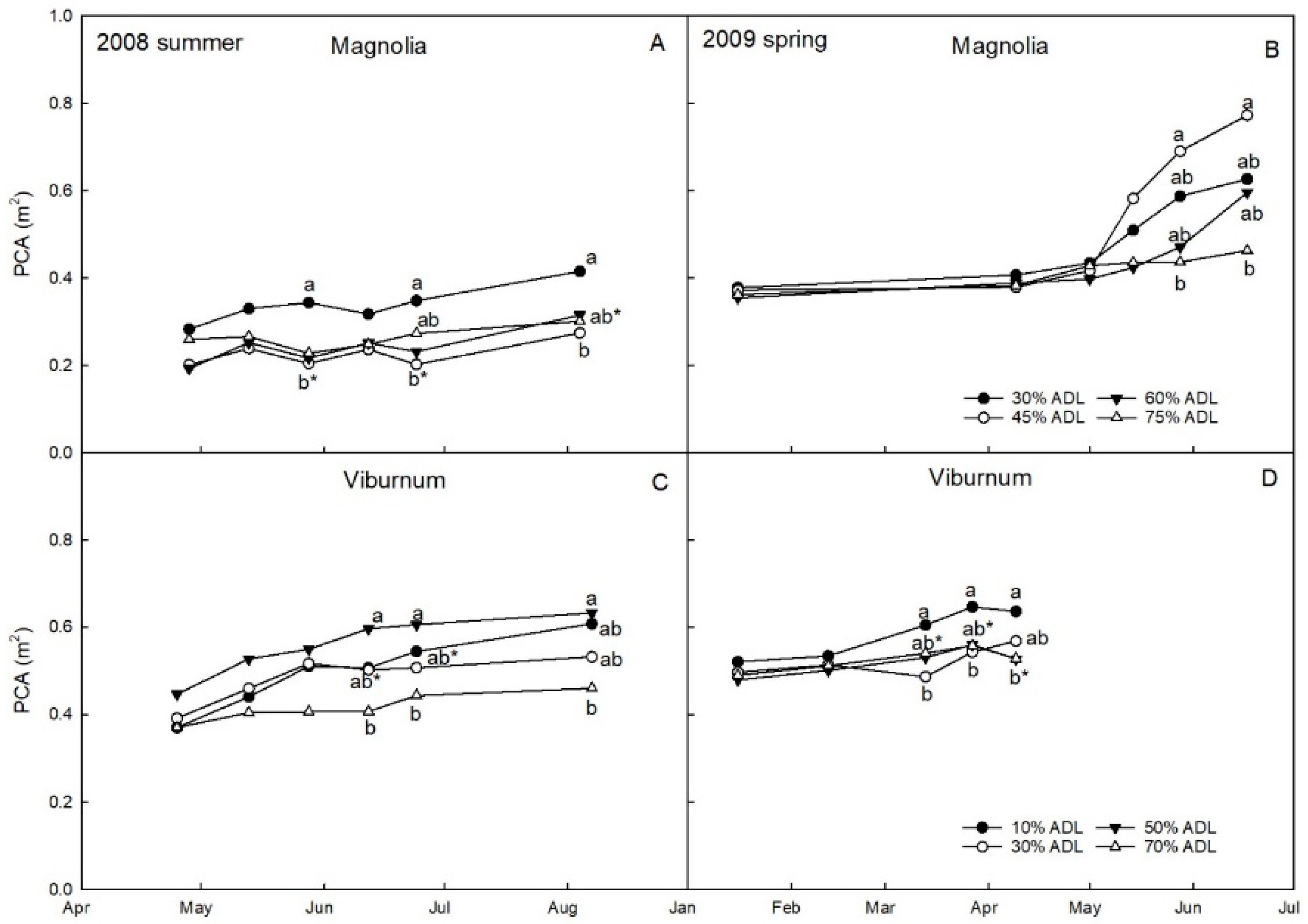
Crown growth increment, measured as projected crown areas (PCA from the inground experiment) over the study periods was modestly affected by greater root-zone drying from less frequent irrigation (Figure 1). Managers typically need a reasonable estimate of the volume of freestanding woody plant water use for irrigation scheduling or planning. Water use volume is the product of the water use rate and the total transpiring leaf area, in particular the sunlit leaf area, that largely drives overall crown transpiration from a freestanding tree. However, a sunlit leaf area and transpiration are difficult to measure and separate from a shaded leaf area [13], so the PCA is a reasonable proxy for the total tree leaf area and transpiration [2,4]. Here, the PCA of both the more frequently irrigated southern magnolia and sweet viburnum (least ADL) was generally greater than the PCA for the less frequently irrigated (greater ADL) treatments, particularly during each species’ seasonal growth flush. The greatest differences were seen during the southern magnolia’s spring growth flush (Figure 1B). Southern magnolia shoot elongation and leaf growth was the greatest from mid-April to late June, as we saw here, continued somewhat during summer (Figure 1A), then stopped from fall through mid-spring. The sweet viburnum peak crown occurs from mid-June until August (Figure 1C) then slows down from fall through early spring (Figure 1D).

Southern magnolia and sweet viburnum water-use normalized to depth units (daily volume water use divided by PCA for a given three-week period) was, like PCA, greatest during the peak growth periods (Figure 2). Differences for the southern magnolia during the summer were not consistent across the four ADL treatments (Figure 2E). During the spring study period (Figure 2F) more frequent irrigation promoted growth (greater PCA) and resulted in increased water use from 1 mm per day in January to above 4 mm per day by June for the 30 and 45% ADL concurrent with increased ET_O, while water use in the 60 and 75% ADL trees were notably lower, with a maximum around 3 mm per day. The brief late May decrease in water use seen in both studies was likely due to expansion by immature leaves that had stomates that may not have been fully functional and transpiring. Reciprocally, ADL treatments had no effect on sweet viburnum water use as it increased from 1 to 3 mm over January to April, but during the summer, sweet viburnum water use in the 10% ADL treatment ranged from 3.5 to 4 mm per day while staying below 2 mm per day for the 50 and 70% ADL treatments. Since the PCA changed little during the summer period, the treatment differences in water were likely due to stress-induced stomatal closure with less frequent irrigation.

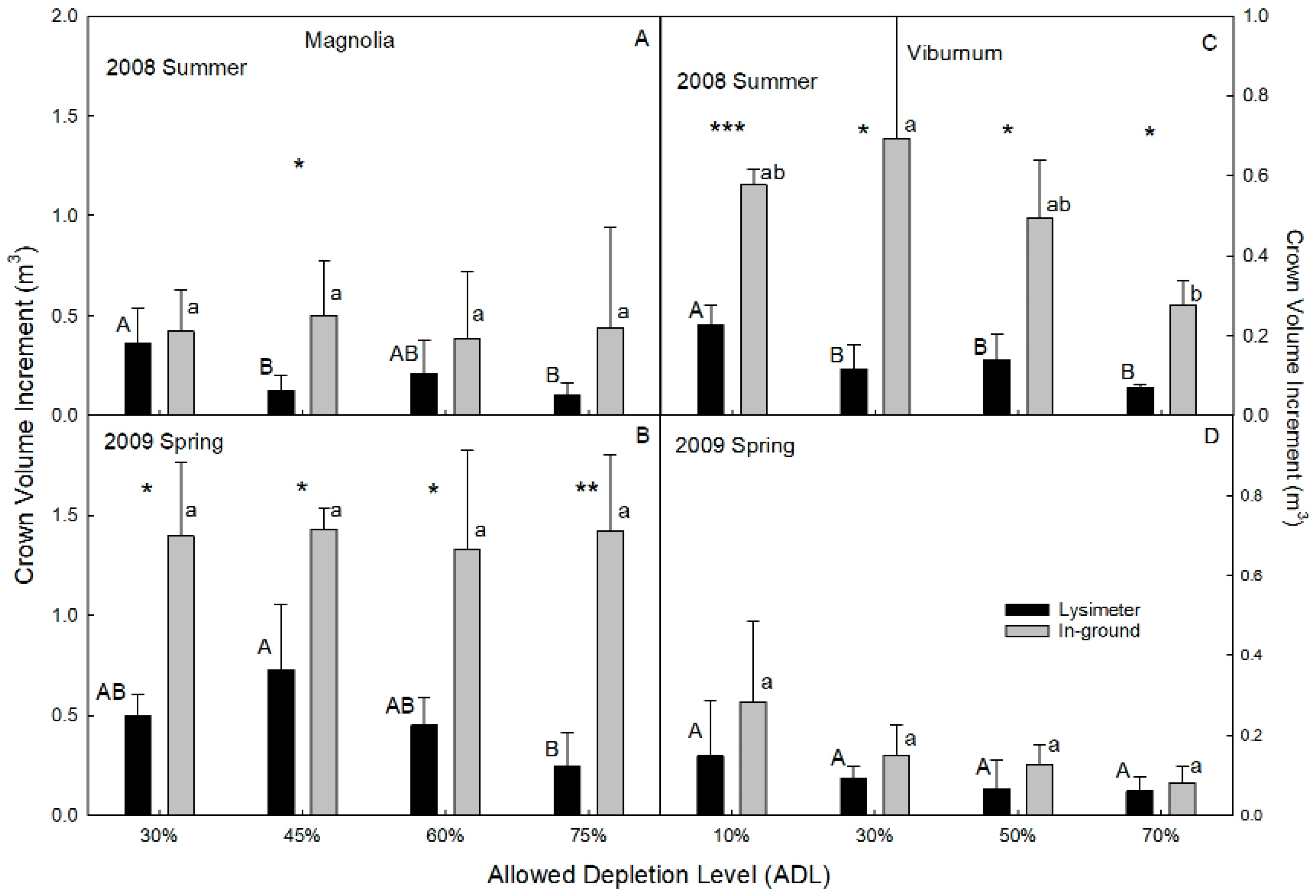
The inground experiment with the same ADL treatments gave more insight into how water stress affected growth in an environment that better approximated a managed landscape. Not surprisingly, both species grew much larger inground than in the lysimeters where root volume was restricted by container size, depending on season of peak growth. But more surprising was that the drought stress treatment effects were minimal (Figure 3). Southern magnolia shoot and leaf growth during spring was up to 4-fold greater inground than in containers due to a vigorous growth flush (Figure 3B), while inground and lysimeter canopy volume increments during the summer were largely minimal (Figure 3A). Conversely, sweet viburnum peak growth was higher during the summer when, again, the inground canopy volume increment was up to 4-fold greater than the lysimeter plants (Figure 3C) but was not different during the somewhat shorter spring experiment in the viburnum canopy increment (Figure 3D). More importantly, drought stress treatments had a relatively minimal impact on inground growth, particularly southern magnolia growth, suggesting that their roots were able to scavenge water despite the close tree spacing of the experimental design. Southern magnolia canopy growth in lysimeter containers under more frequent irrigation at 30% ADL was larger both seasons, but irrigation frequency had no impact on inground southern magnolia canopy growth in either season. Less frequent irrigation did affect sweet viburnum canopy increments during peak summer growth, but there was no ADL treatment effect during the spring treatment. Interestingly, during the peak growth summer experiment, the sweet viburnum canopy increment at 30% ADL was larger than for the other irrigation treatments.

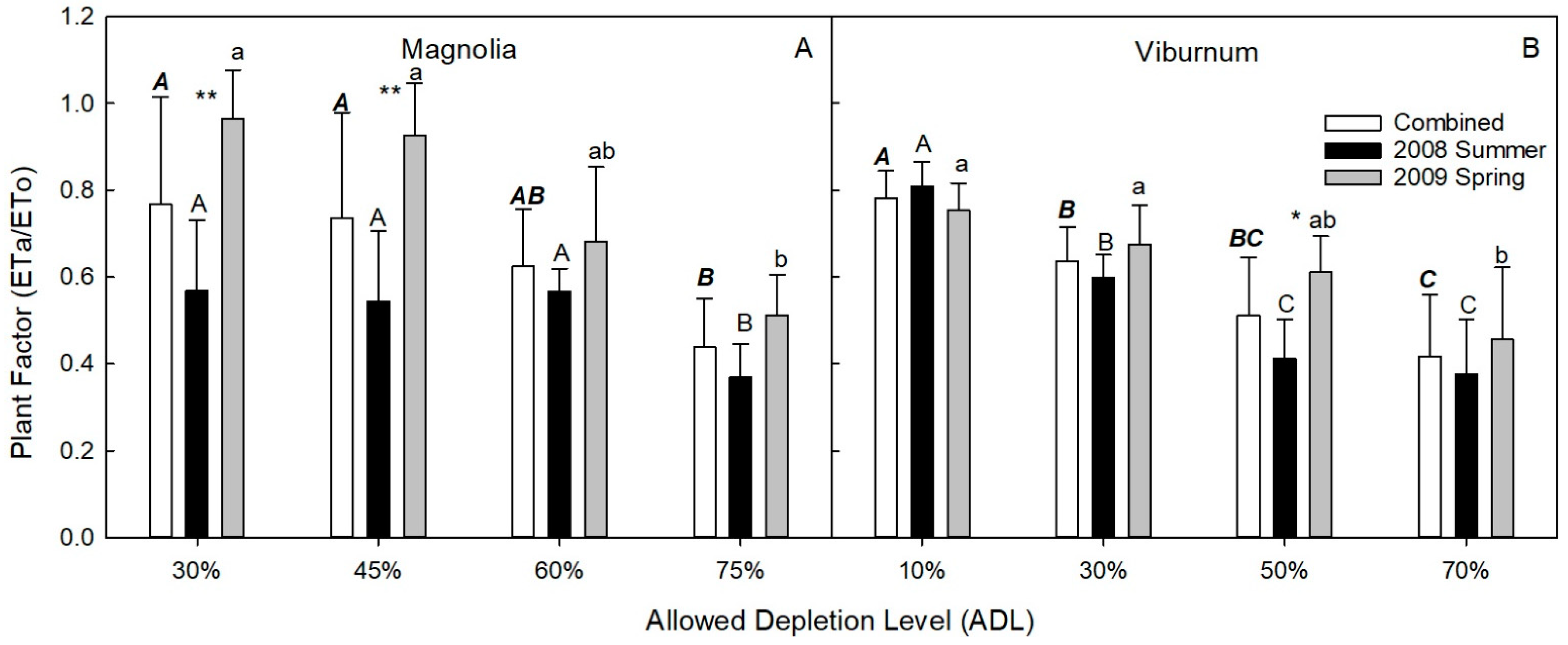
The PF, or the ratio of actual water use ETa in depth units to ET_O, allows landscape and water managers and designers to estimate water demand of a plant or a landscape. Here, irrigation frequency did have an impact on the PF of both the southern magnolia and sweet viburnum within either of the seasonal experiments, as PF values generally decreased as irrigation frequency decreased (greater ADL) but varied by season and species (Figure 4). The southern magnolia PF was the highest in spring—consistent with maximum growth period—with more frequent irrigation (30 and 45% ADL) but was 30% less during summer with less pronounced differences among ADL treatments. Sweet viburnum was somewhat the reverse, as PF differences among the ADL treatments was greatest during its peak growth period, again the highest with the least ADL (more frequent irrigation) and seasonal differences were less than for the magnolia. The combined magnolia PF values at the two wettest ADL treatments (more frequent irrigation) for both species (75) represents a practical balance between the two seasons as a yearly average PF. For the southern magnolia, an average 0.7 PF well represented the two more frequently irrigated treatments (30 and 45% ADL), while for the sweet viburnum combined PF values were 0.78 at 10% ADL and 0.68 at 30% ADL.

4. Discussion

Currently, there are three ways to control irrigation automatically through time clocks: manual changes with season, soil water sensors, and weather-based (ET_O) automatic control based on water budgets, which require a PF value. Time clocks are inexpensive and easy to set up, but frequently adjusting for seasonal—let alone day-to-day—changes in rainfall and ETo is impractical. Soil water sensors wired to a time clock can control irrigation by signaling when to turn on and shut down irrigation by detecting a changes in soil water content relative to a threshold, such as an ADL. Requiring more initial setup are a time clock connected to the daily input of ETo values, and an irrigation duration and frequency set based on ETo x PF to estimate how fast water is being used combined with ADL that sets the threshold of water depletion to trigger irrigation to refill the root zone. In a fully exposed landscape, rainfall needs to factor into a water budget, particularly in a humid climate such as in the southeastern U.S. Many states have weather station networks that provide ET_O data that can be wirelessly digested by appropriately engineering the times.

Here we show that the southern magnolia and sweet viburnum can tolerate moderate root-zone drying (ADL level) while maintaining canopy growth and appearance. Both species had acceptable appearances for all ADL treatments except 75% ADL for the southern magnolia and 70% ADL for the sweet viburnum in lysimeters (data not shown). In dry climates of limited water where landscape conservation is important, managers can maximize water use efficiency though deficit irrigation, or irrigating below plant water demand and imposing mild water stress without affecting yield [14], particularly when applied during growth stages when yield is less sensitive to water stress [15]. Unlike crops, aesthetic appearance rather than yield is of more importance for landscape plants [16], and most non-turf urban landscape plants can maintain acceptable functionality and aesthetic performance even at some level of deficit irrigation [16,17,18], resulting in significant water savings [19]. In this study, greater root-zone drying at 50–60% ADL functioned as a deficit irrigation threshold where both species may have been under mild to moderate water stress but growth and appearance were marginally affected.

The other part of an efficient landscape water budget is the rate of root-zone water depletion, which is daily plant water demand estimated as ET_O x PF. The PF is an important index for irrigation control in urban landscapes, both for single or grouped plantings [1,2,10,20,21]. However, research on PF values has been mostly conducted in arid climates, and recommended PF values are best applied in similar dry climates, but research of PF values of trees and shrubs in a humid climate is limited. Based on the results here, we suggest PF values for southern magnolia of 0.7 during vigorous growth in late spring; and 0.5–0.6 for the rest of the year. For sweet viburnum, PF values of 0.5–0.6 would be reasonable during the spring dry season in a monsoonal climate, but during the summer monsoons, rainfall is frequent enough that irrigation typically is not needed except for extreme drought. This recommendation is within the 0.5 to 0.7 range reported by Pannkuk [22] for the similar climate of south Texas for mixed turf/woody landscapes using drainage lysimeters and for the turf and woody plant PFs [2] suggested for humid climates.

If faster growth rates and larger plant sizes are the goal of a landscape, we do not recommend deficit irrigation. Southern magnolia is typically used as a free-standing specimen tree in landscapes, so rapid canopy growth would be expected until an expected size is reached. Sweet viburnum has similar performance expectations, as it is typically used as a hedge to define borders and block unwanted sights and sounds, so rapid canopy growth would also be the performance expectation until hedge canopy closure is reached. As such, for recently installed landscapes during establishment where deficit irrigation and mild-to-moderate water stress is undesirable, we recommend a more generous water budget: 30% ADL and PF values of 0.7 of ET_O. For the established southern magnolia, which has peak canopy growth in mid-late spring and is used to monsoonal drought, a deficit irrigation of 50% ADL would be appropriate until the start of summer monsoons. For sweet viburnum, frequent, intense rainfall during a typical summer monsoon in a subtropical climate would obviate the need for deficit irrigation; established sweet viburnum hedges with summer growth flush would likely meet performance expectations without irrigation except for extremely dry springs where 0.5 ADL and 0.7 PF would be appropriate.

5. Conclusions

On-the-ground landscape managers can most directly use these results to schedule the irrigation of these two species and similar species adapted to seasonally wet and dry climates. The larger target audience for these results is the design, planning, and supplier community responsible for managing water in urban landscapes. Landscape architects and designers can create water-budget benchmarks based on plant factors together with a landscaped area and local ETo. Furthermore, water agencies can use PFs to track end-user consumption that can be compared against water-budget benchmarks to develop policies that educate and encourage informed conservation practices [23]. Even in a humid climate such as the southeastern U.S., especially Florida, increasing temperatures and dry periods are increasing the demand for landscape irrigation and so making wise and informed conservation policies more important [24].

The results presented here will not necessarily apply to all woody plants that can be grown in humid to subtropical climates. During a drought, PF values can be scaled back for landscapes with native southeastern U.S. species that are likely to be adapted to seasonably dry conditions, such as the southern magnolia and sweet viburnum. However, the many other landscape species that can grow in a humid climate, especially a subtropical one like Florida’s, include many that may have similar water uses but have desiccation-intolerant foliage and shallow root systems that would make them susceptible to damage during a drought and therefore inappropriate for a landscape. A classification of landscape species for drought tolerance, such as in the University of Florida’s Florida-Friendly Landscaping program, is a key to complementing proper landscape water management design, planning and irrigation scheduling [25].

These results also reinforce the concept of a PF for use in landscape irrigation. The crop coefficient Kc and PF both scale down local evaporative demand conditions captured by ETo to that of the plant of interest, and Kc encompasses PF values to an extent [26]. Because of crop uniformity and a limited number of species, research has developed reasonably precise and seasonally accurate Kc values to schedule when and how much to irrigate for much of high-value agriculture. In landscapes, more species and spatial and microclimate diversity limit precision, so the PF represents a more general but useful and accessible tool for scaling a local ETo to the landscape for planning and management purposes. Simply put, a scientifically based PF, such as presented here, is easier for the urban water management community to grasp.

References

- Hilaire, S.R.; Arnold, M.; Wilkerson, D.C.; Devitt, D.A.; Hurd, B.H.; Lesikar, B.J.; Zoldoske, D.F. Efficient water use in residential urban landscapes. HortScience 2008, 43, 2081–2092. [Google Scholar] [CrossRef]
- Kjelgren, R.; Beeson, R.C.; Pittenger, D.R.; Montague, D.T. Simplified landscape irrigation demand estimation: SLIDE rules. Appl. Eng. Agric. 2016, 32, 363–378. [Google Scholar] [CrossRef]
- Beeson, R.C.; Duong, H.; Kjelgren, R. Developing a simple water use model of Ilex × ‘Nellie R. Stevens’ from liners to four meter tall trees. J. Agric. Stud. 2017, 5. [Google Scholar] [CrossRef] [Green Version]
- Beeson, R.C.; Duong, H.; Kjelgren, R. Water use of juvenile Live Oak (Quercus virginiana) trees over five years in a humid climate. Open J. For. 2018, 8, 1–14. [Google Scholar] [CrossRef] [Green Version]
- Koesera, A.K.; Gilman, E.F.; Paz, M.; Harchick, C. Factors influencing urban tree planting program growth and survival in Florida, United States. Urban For. Green 2014, 13, 655–661. [Google Scholar] [CrossRef]
- Scheiber, S.M.; Gilman, E.F.; Sandrock, D.R.; Paz, M.; Wiese, C.; Brennan, M.M. Postestablishment landscape performance of Florida native and exotic shrubs under irrigated and nonirrigated conditions. HortTechnology 2008, 18, 59–67. [Google Scholar] [CrossRef] [Green Version]
- Shober, A.L.; Moore, K.A.; West, N.G.; Wiese, C.; Hasine, G.; Denny, G.; Knox, G. Growth and quality response of woody shrubs to Nitrogen fertilization rates during landscape establishment in Florida. HortTechnology 2013, 23, 898–904. [Google Scholar] [CrossRef] [Green Version]
- Warsaw, A.L.; Fernandez, R.T.; Cregg, B.M.; Andresen, J.A. Water conservation, growth, and water use efficiency of container-grown woody ornamentals irrigated based on daily water use. HortScience 2009, 44, 1308–1318. [Google Scholar] [CrossRef]
- Beeson, R.C. Weighing lysimeter systems for quantifying water use and studies of controlled water stress for crops grown in low bulk density substrates. Agric. Water Man. 2011, 98, 967–976. [Google Scholar] [CrossRef]
- Allen, R.G.; Pereira, L.S.; Raes, D.; Smith, M. Crop Evapotranspiration-Guidelines for Computing Crop Water Requirements-FAO Irrigation and Drainage; Food and Agriculture Organisation of the United Nations: Rome, Italy, 1998; p. 56. [Google Scholar]
- Ringgaard, R.; Herbst, M.; Friborg, T. Partitioning of forest evapotranspiration: The impact of edge effects and canopy structure. Agric. For. Meteorol. 2012, 166, 86–97. [Google Scholar] [CrossRef]
- Gunston, H.; Batchelor, C.H. A comparison of the Priestley-Taylor and Penman methods for estimating reference crop evapotranspiration in tropical countries. Agric. Water Man. 1983, 6, 65–77. [Google Scholar] [CrossRef]
- Pereira, A.R.; Green, S.; Nova, N.A.V. Relationships between single tree canopy and grass net radiations. Agric. For. Meteorol. 2007, 142, 45–49. [Google Scholar] [CrossRef]
- Geerts, S.; Raes, D. Deficit irrigation as an on-farm strategy to maximize crop water productivity in dry areas. Agric. Water Manag. 2009, 96, 1275–1284. [Google Scholar] [CrossRef] [Green Version]
- Cui, N.B.; Du, T.S.; Kang, S.Z.; Li, F.S.; Zhang, J.H.; Wang, M.X.; Li, Z.J. Regulated deficit irrigation improved fruit quality and water use efficiency of pear-jujube trees. Agric. Water Manag. 2008, 95, 489–497. [Google Scholar] [CrossRef]
- Kjelgren, R.; Rupp, L.; Kilgren, D. Water conservation in urban landscapes. HortScience 2000, 35, 1037–1043. [Google Scholar] [CrossRef] [Green Version]
- Montague, T.; Kjelgren, R.; Allen, R.; Wester, D. Water loss estimates for five recently transplanted landscape tree species in a semi-arid climate. J. Environ. Hortic. 2004, 22, 189–196. [Google Scholar] [CrossRef]
- Pittenger, D.R.; Shaw, D.A.; Hodel, D.R.; Holt, D.B. Responses of landscape groundcovers to minimum irrigation. J. Environ. Hortic. 2001, 19, 78–84. [Google Scholar] [CrossRef]
- Hartin, J.S.; Fujino, D.W.; Oki, L.R.; Reid, S.K.; Ingels, C.A.; Haver, D. Water requirements of landscape plants studies conducted by the University of California researchers. HortTechnology 2001, 28, 422–426. [Google Scholar] [CrossRef] [Green Version]
- Costello, L.R.; Matheny, N.P.; Clark, J.R. A Guide to Estimating Irrigation Water Needs of Landscape Plantings in California, the Landscape Coefficient Method and WUCOLS III; University of California Cooperative Extension, California Department of Water Resources: Sacramento, CA, USA, 2000; Available online: cimis.water.ca.gov/Content/PDF/wucols00.pdf (accessed on 10 June 2020).
- Allen, R.G.; Walter, I.; Elliot, R.; Howell, T. The American Society of Civil Engineers Standardized Reference Evapotranspiration Equation; American Society of Civil Engineers: Reston, VA, USA, 2001. [Google Scholar] [CrossRef]
- Pannkuk, T.R.; White, R.H.; Steinke, K.; Aitkenhead-Peterson, J.A.; Chalmers, D.R.; Thomas, J.C. Landscape coefficients for single-and mixed-species landscapes. HortScience 2010, 45, 1529–1533. [Google Scholar] [CrossRef] [Green Version]
- Glenn, D.; Endter-Wada, J.L.; Kjelgren, R.; Neale, C.M. Tools for evaluating and monitoring effectiveness of urban landscape water conservation interventions and programs. Landsc. Urban. Plann. 2015, 139, 82–93. [Google Scholar] [CrossRef] [Green Version]
- Williams, A.P.; Cook, B.I.; Smerdon, J.E.; Bishop, D.A.; Seager, R.; Mankin, J.S. The 2016 Southeastern U.S. drought: An extreme departure from centennial wetting and cooling. J. Geophys. Res. Atmos. 2017, 122, 10888–10905. [Google Scholar] [CrossRef] [PubMed]
- Clem, T.B.; Hansen, G.A.; Dukes, M.D.; Momol, E.; Kruse, J.; Harchick, C.; Bossart, J. Sustainable residential landscapes in Florida: Controlled comparison of traditional versus Florida-friendly landscaping. J. Irrig. Drain. Eng. 2021, 147. [Google Scholar] [CrossRef]
- Allen, R.G.; Dukes, M.D.; Snyder, R.L.; Kjelgren, R.; Kilic, A.A. A review of landscape water requirements using a multicomponent landscape coefficient. Trans. ASABE 2020, 63, 2039–2058. [Google Scholar] [CrossRef]
Figure 1.
Projected crown area (PCA) increase during the summer and spring study periods for Southern magnolia (Magnolia grandiflora; n = 4) and sweet viburnum (Viburnum odoratissiumum; n = 3) growing in lysimeter containers and subjected to four levels of allowable soil water depletion levels (ADL). (A,B), Projected Crown Area (PCA) of magnolia during the 2008 summer and 2009 spring; (C,D) PCA of viburnum during the 2008 summer and 2009 spring. Dates with mean separation letters (a, b, ab) are significantly different at p < 0.05. Letters with an asterisk indicate adjacent date points that are not significantly different.
Figure 2.
(A–D) Atmospheric conditions during two experimental periods, summer of 2008 and spring of 2009, as well as (E–H) woody plant water use for southern magnolia (Magnolia grandiflora; n = 4) and sweet viburnum (Viburnum odoratissimum; n = 3) growing in lysimeter containers and subjected to four levels of allowable soil water depletion levels (ADLs). (A,B), Daily reference evapotranspiration (ETO) and air temperature; (C,D), incoming photosynthetically active radiation and vapor pressure deficit; (E–H), normalized ETA (measured volumetric water use ÷ PCA) with a 10-day rolling ETA (lines) and actual ETA (data marks) on the day of PCA measurement for both periods. Dates showing mean separation letters (a, b, c) are significantly different at p < 0.05. Letters with an asterisk indicate adjacent data points that are not significantly different.
Figure 3.
Effect of allowable depletion level (ADL) on crown volume (projected crown area x plant height) during the summer and spring study periods for southern magnolia (Magnolia grandiflora, n = 4) and sweet viburnum (Viburnum odoratissimum, n = 3) growing in lysimeter containers and subjected to four levels of allowable soil water depletion levels at the termination of the summer and spring studies. (A,B), Crown Volume Increment (CVI) in cubic meters of magnolia during the 2008 summer and 2009 spring; (C,D) CVI of viburnum during the 2008 summer and 2009 spring. Asterisks above the summer and spring experiment columns indicate significant seasonal differences at the 0.001 (***), 0.01 (**) and 0.05 (*) probability levels. Columns showing mean separation letters a, b or A, B are significantly different at p < 0.05 among the ADL treatments for the inground and lysimeter plants, respectively.
Figure 4.
Effect of allowable depletion level (ADL) on plant factor (normalized lysimeter plant water use ETa ÷ reference evapotranspiration ETO) for the southern magnolia (Magnolia grandiflora, n = 4) and sweet viburnum (Viburnum odoratissimum, n = 3) growing in lysimeter containers and subjected to four levels of allowable soil water depletion levels (ADL) for spring and summer study periods, and combined for an average PF (n = 8, 6 respectively). (A), Plant Factor of magnolia in the 2008 summer, 2009 spring and from both periods of time combined contrasted with Allowed Depletion Levels (ADL); (B), Plant Factor of viburnum in the 2008 summer, 2009 spring and from both periods of time combined contrasted with ADL; Asterisks above the summer and spring experiment columns indicate significant seasonal differences at the 0.01 (**) and 0.05 (*) probability level. Columns showing mean separation letters ab, A–B or A–B are significantly different at p < 0.05 across ADL treatments for the 2008 summer, 2009 spring, and both periods combined, respectively.
Publisher’s Note: MDPI stays neutral with regard to jurisdictional claims in published maps and institutional affiliations. |
© 2021 by the authors. Licensee MDPI, Basel, Switzerland. This article is an open access article distributed under the terms and conditions of the Creative Commons Attribution (CC BY) license (https://creativecommons.org/licenses/by/4.0/).
Share and Cite
MDPI and ACS Style
Sun, H.; Kjelgren, R.; Dukes, M.D.; Beeson, R.C. Magnolia and Viburnum Plant Factors at Different Growing Seasons and Allowed Depletion Levels in a Monsoonal Climate. Water 2021, 13, 1744. https://doi.org/10.3390/w13131744
AMA Style
Sun H, Kjelgren R, Dukes MD, Beeson RC. Magnolia and Viburnum Plant Factors at Different Growing Seasons and Allowed Depletion Levels in a Monsoonal Climate. Water. 2021; 13(13):1744. https://doi.org/10.3390/w13131744
Chicago/Turabian StyleSun, Hongyan, Roger Kjelgren, Michael D. Dukes, and Richard C. Beeson. 2021. "Magnolia and Viburnum Plant Factors at Different Growing Seasons and Allowed Depletion Levels in a Monsoonal Climate" Water 13, no. 13: 1744. https://doi.org/10.3390/w13131744
Note that from the first issue of 2016, this journal uses article numbers instead of page numbers. See further details here.