
A New Dam-Break Outflow-Rate Concept and Its Installation to a Hydro-Morphodynamics Simulation Model Based on FDM (An Example on Amagase Dam of Japan)


1
Graduate School of Science and Technology, Tokai University, Kanagawa 259-1292, Japan
2
Department of Civil Engineering, Tokai University, Kanagawa 259-1292, Japan
*
Author to whom correspondence should be addressed.
Water 2021, 13(13), 1759; https://doi.org/10.3390/w13131759
Submission received: 4 May 2021
/
Revised: 16 June 2021
/
Accepted: 21 June 2021
/
Published: 25 June 2021
(This article belongs to the Special Issue Advances in Dam-Break Modeling for Flood Hazard Mitigation: Theory, Numerical Models, and Applications in Hydraulic Engineering)
Abstract
:Dams are constructed to benefit humans; however, dam-break disasters are unpredictable and inevitable leading to economic and human life losses. The sequential catastrophe of a dam break directly depends on its outflow hydrograph and the extent of population centers that are located downstream of an affected dam. The population density of the cities located in the vicinity of dams has increased in recent times and since a dam break hydrograph relies on many uncertainties and complexities in devising a dam-break outflow hydrograph, more researches for the accurate estimation of a dam-break flood propagation, extent and topography change becomes valuable; therefore, in this paper, the authors propose a novel and simplified dam-break outflow rate equation that is applicable for sudden-partial dam breaks. The proposed equation is extensively affected by a dam-break shape. Therefore, the inference of a dam-break shape on a dam-break outflow rate is investigated in the current study by executing hydraulic experiments in a long, dry bed, frictionless and rectangular water channel connected to a finite water tank to acquire a mean break-shape factor. The proposed equation is further validated by regenerating the Malpasset dam-break hydrograph and comparing it to the existing methods and also by installing it on an existing 2D hydro-morphodynamics flood simulation model. Finally, Amagase Dam’s (arch-reaction dam in Japan) break simulation is executed as a case study. The results of the simulations revealed that the greater the height of a dam-break section, the more devastating its flood consequences would be.
1. Introduction
As water is stored behind a dam, enormous potential energy is formed that in the case of a dam-break, devastating catastrophe may follow [1] especially, when densely populated cities are located downstream of a dam [2], in the last two decades, floods resulting from dam breaks are responsible for some of the most devastating man-made disasters. Therefore, every effort to further reduce the severe effects of a dam break and generating a better forecast of its flood extent in the tailwater areas is of immense value [3].
The development of effective emergency action plans and the design of an early warning system that might reduce or eliminate the consequences of a dam break requires its inundation information downstream [4]. The development of the inundation information from a dam break consists of three steps: the routing of the inflow flood through a reservoir, estimating the dam breach characteristics and the downstream flood routing [5]. Out of these three steps, estimating the characteristics and parameters of the dam breach contains the greatest uncertainties of all aspects of dam-break [6]. Therefore, in this paper, the authors present a simplified novel approach relevant to sudden-partial dam-break outflow rate for non-erodible type dams.
Generating precise dam-break hydrographs has been a major concern since the end of the 10th century [3]. The first documented experimental dam-break experiment in a channel might be the one proposed by Bazin [7], following which, Ritter [8], derived an analytical solution of the famous one-dimensional De-Saint Venart equation for sudden dam-breaks. Later on, Su and Barnes [9], extended Ritter’s solution considering the effect of different channel cross-sections and proposed a useful power type equation for this phenomenon. However, until recent years, very few advances have been reported to address the dam-break problem [3].
In most dam-break studies, the reservoir is usually assumed as a long infinite water supply until Aureli et al. [10], presented useful approaches by numerically solving the Ritter, and Su and Barnes [9] methods in combination, as well as considering dam-break bathymetry effects on the produced outflow hydrograph. Fundamentally, an outflow hydrograph is affected by the bathymetry of a dam, valley shape, dam height and shape and extension of the breach. In the papers [3,11,12,13], the effects of dam bathymetry on the dam-break hydrograph have been evaluated and many more researchers have concentrated on the breach formation shape and breach formation time [14].
In all studies predating [3], all researchers had assumed a total dam-break scenario which is not realistic and does not take into account the types of dams that can be partially breached. Concerning this fact, Piloti et al. [3] and Aureli et al. [10] proposed methods to address sudden partial dam breaks. However, based on the equation (23) of Aureli et al. [10] and equation (19) of Pilotti et al. [3] the details of the storage-depth curve of the reservoir are necessary to precisely calculate the outflow hydrograph.
In the practical scenario, the storage-depth curves might either not be available or difficult to acquire for some existing dams. Hence to overcome this issue, the authors propose a new dam-break outflow rate equation that requires only the height of a dam for calculating a dam break outflow rate. The proposed equation is applicable to many concrete dam types. However, because the proposed equation is extensively affected by the dam-break cross-section a flow rate coefficient (break shape factor) must be initially decided. In the present work, for the arch dams (dams with thin width) a mean shape factor is acquired after executing many hydraulic experiments in a channel.
To show the validity of the proposed equation, the hydrograph of the famous Malpasset dam-break that happened in 1959 in Fréjus city of France, is generated and compared to that of [10]. The results reveal that the proposed equation comparatively produces a higher peak discharge and a faster emptying time. Finally, the inference of a dam-break height and width on the extent in inundation area and initial flood wave velocity is investigated by executing many dam-break simulations on the Amagase dam which is a concrete arch-reaction dam in Japan. The results suggest that, as the break section’s height increases, the inundation extent and initial flood velocity increase even if the break cross-sectional area tends to remain the same.
2. Calculation Methods
2.1. New Model of Dam-Break Out-Flow Rate
For the development of the dam-break hydrograph, a finite volume reservoir with a surface area of is assumed with a break section of width and heigh . shown in Figure 1a,b. The shape of a break section can vary from a rectangle to a triangle depending on the shape of a proposed dam valley. Since in this paper, it is intended to develop a dam-break outflow rate equation that is independent of a dam’s stage-discharge curve, an imaginary coefficient is assumed for the dam-break section. is measured from the water surface level of a dam’s reservoir and it is many times the height of a dam. If is set to a very high value compared to the respected dam height, it replicates an almost rectangular dam-break cross-section, and vice versa, if this value is set to a relatively small value, it replicates a trapezoidal and triangle reservoir cross-section. Therefore, the proposed equation can produce the outflow rate of a dam break with different cross-sections.
The run-off rate from the dam lake in the case that the overflow height is assumed constant (water supply is infinite) can be calculated using the below equations:
Here, is the discharge rate; is the final depth of a break section; is the earth’s gravitational force; and are the width and minute height of the break portion at depth ; is falling depth of water surface in a dam lake after a break; is the flow rate coefficient; is the imaginary depth from the dam crown level as shown in Figure 1b.
Since the case of finite water supply from a dam lake is more realistic in the actual dam-break cases, in Equation (3) is substituted with . Here, is the run-off elapse time (sec). In the following, equations for dam-break outflow rate (), and the total volume of discharge (), are developed with considering the case of finite water supply from a dam reservoir;
Now, substituting with gives the below equation for ;
Here, is the cumulative time from the start of the calculations.
2.2. Existing Numerical Simulation Model
For the development of the inundation information and topographical change due to a long-wave flood such as a tsunami or dam-break, the numerical simulation model of Ca et al. [15] is used. The model was developed using the following detailed formulas.
2.2.1. Numerical Model for Fluid Motion
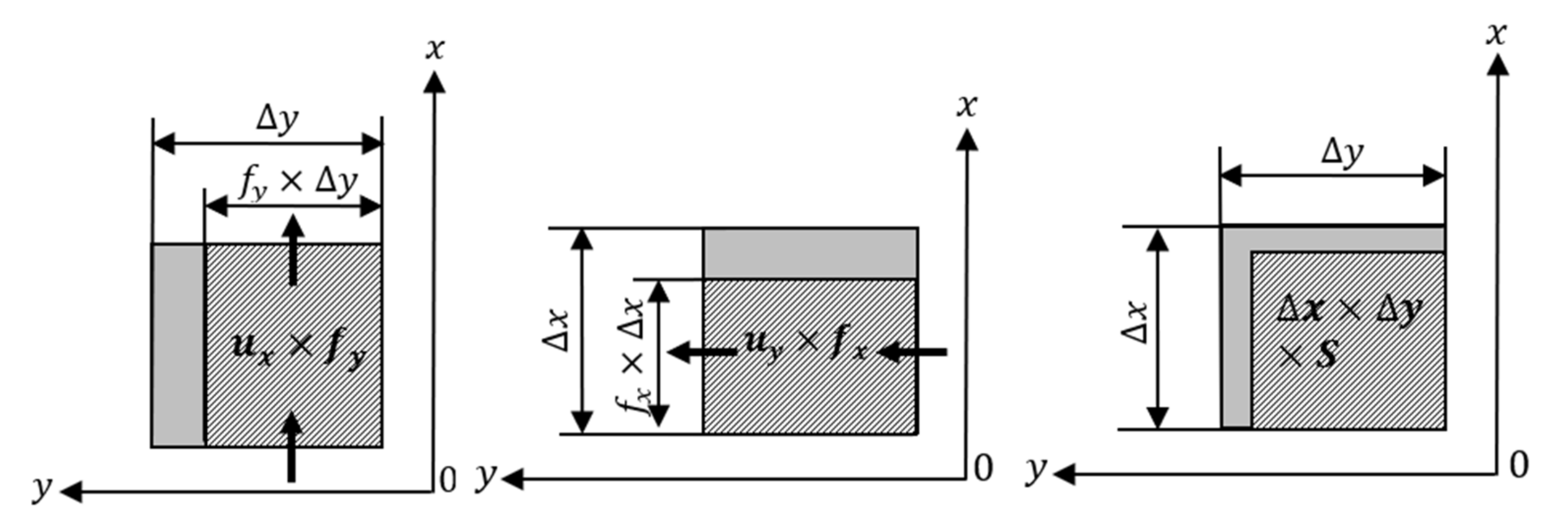
The numerical model used for long-wave flood simulations in this paper is based on a continuity equation of fluid (Equation (14)) and two-dimensional nonlinear long-wave equations (Equations (15) and (16)), and these governing equations are solved by finite difference method using the Crank-Nicholson scheme.
Here, and are the horizontal fluid fluxes in the directions respectively; is the water surface elevation. are the direction ratios of the wet portion in a calculation mesh; is the area ratio of the wet portion in a calculation mesh see Figure 2; is the water depth (from the static water surface +); is the gravitational acceleration; is the eddy viscosity coefficient; is the ground surface friction coefficient; and is the compound value of and .
To calculate the eddy viscosity coefficient and the ground surface friction coefficient, the following equations are used;
Here, and are the flow velocity in and directions; equals (0.1); is Manning’s roughness coefficient; is the building ratio (= the ratio of the area of all vertical objects such as houses and trees to the mesh area). is the weighted average roughness coefficient of areas such as farms, roads and waste and wetlands, respectively, with relative roughness coefficients of [16].
2.2.2. Numerical Model for Topographical Change
The topographical change based on sediment transport by the flow can be expressed by using the continuity equation, Equation (21);
Here, is the ground surface elevation; are respectively the bed-load rate per unit width in directions; is the deposition rate of the suspended load; is the entrainment rate of the suspended load from the bed; and is the porosity of the sediment.
(1) Modeling of qx and qy on Bed-load Transport
For evaluation of the bed-load rate, Ribberink’s formula [17], shown in Equation (22) is used. Yokoyama et al. [18] performed many calculations of scouring by flow and wave using indoor and outdoor data on sand and gravel with a diameter range of 0.2~10 mm and found that accurate results can be obtained using this formula.
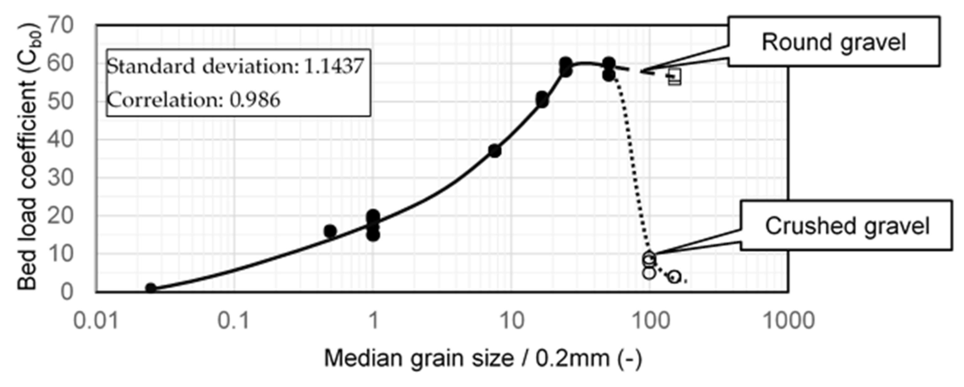
Here, qbi is the bed-load transport rate per unit width in the i direction; Cb is the bed-load transport coefficient determined by verification simulations; however, the authors by performing many hydraulic experiments, developed useful diagrams to acquire the value of this coefficient, refer to Figures 3–5 [19]; θs(t) is the Shields parameter in the i direction; θsc is the critical Shields number, calculated by using the equation of van Rijn, [20]; Δ is the relative density of the sand; g is the gravitational acceleration; D50 is the median diameter of the sediment.
(2) Modeling of on Suspended Load Transport
During a long wave flood, it is necessary to consider the influence of suspended load transport. The deposition rate of the suspended load and the entrainment rate from the bed was evaluated using Equation (23) based on the vertical distribution of suspended load concentration:
Here, ws is the settling velocity of suspended particles which can be calculated using Equation (24) [21,22,23]; C(z) is the suspended load concentration and can be calculated using Equation (25) [24], under the assumption of the sheet flow condition for the whole area; vt is the eddy viscosity.
Here, is the kinematic viscosity of water; is van Rijin’s dimensionless particle parameter; is Karman’s constant ; is the friction velocity; and are estimated using Equation (26) [25].
3. Methods for Evaluation of Empirical Coefficients
3.1. Evaluation of the Break-Shape Coefficient of the Outflow Rate Equation
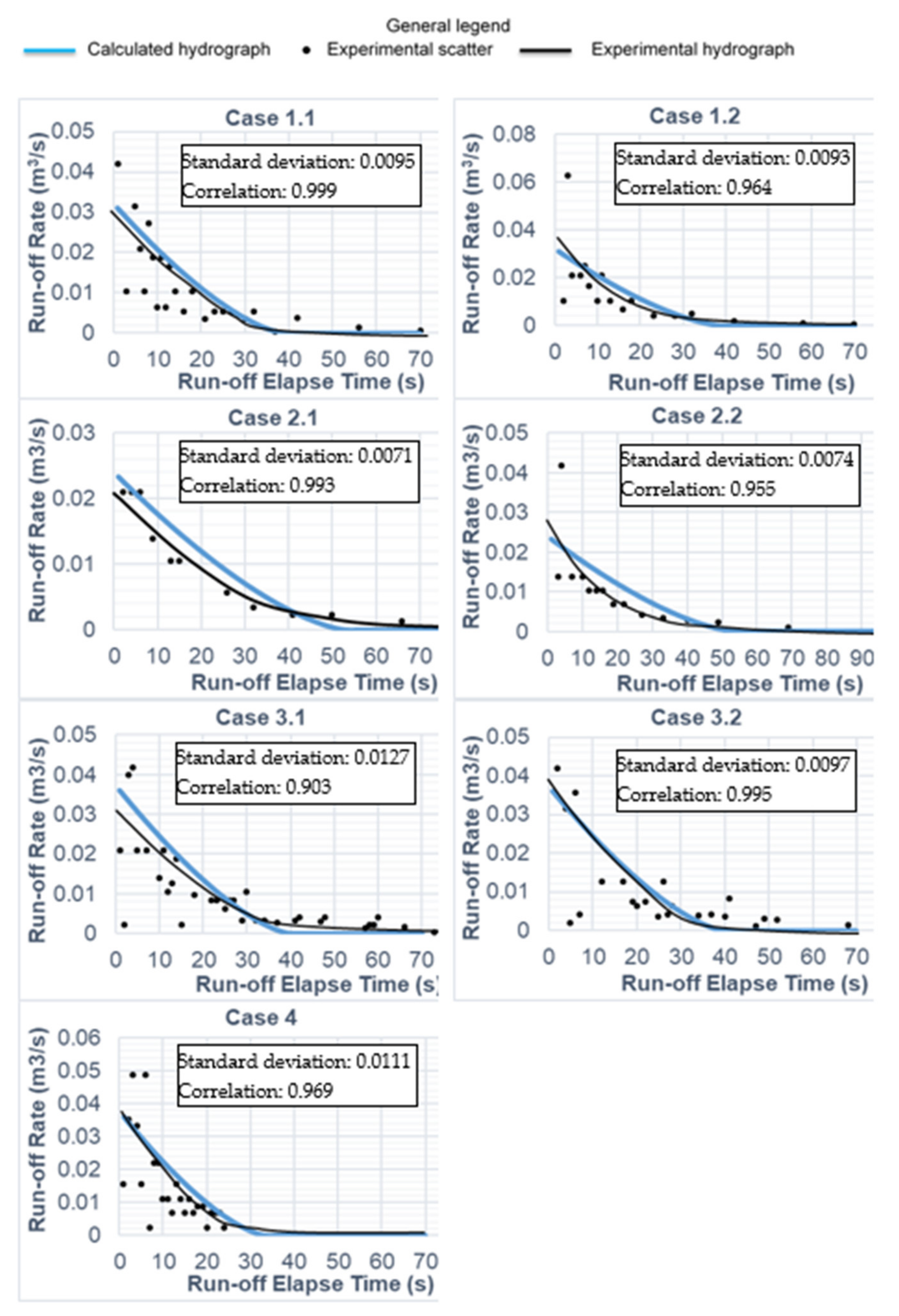
For the newly proposed outflow rate equation, (Equation (4)) the coefficient has a great impact on a calculated hydrograph. This coefficient depends on many variables, i.e., dam bathymetry, type of break, break dimensions and dam width and height. Initially, the dam-break section’s impact on this coefficient is evaluated in this paper, by performing many hydraulic experiments. Figure 3a,b shows the apparatus and experimental arrangements respectively. On the left-hand side of the apparatus, there is a water tank reserve acting as a dam reservoir, at the downstream, there is a dry-bed water channel of 0.5 m in width, 0.4 m in height and 12 m in length. At the one-meter section from the reservoir, two layers of acryl plates of one centimeter in thickness are placed and sealed using silicon glue. The two plates are arranged as both of them are cut to the desired section, listed in Table 1. One other plate placed in between these two acts as a gate where grease is used as a lubricant in between the plates to let one open the gate abruptly. This complies with the objective of sudden partial dam-break. From these experiments, it is intended to develop the hydrographs, therefore, using a digital camera which is focused on the scale bar located about 50 cm upstream of the acryl plates; the whole process of the experiments is recorded. Using this arrangement, one can measure the change in water height behind the dam, and because previously, the bathymetry measurements (reservoir surface area) are taken, the discharge rate is calculated. Figure 4 shows the calculated and measured hydrographs, where the standard deviation and correlation value between the calculated hydrograph and experimental hydrograph are also presented for each of the experimented cases. For calculated hydrographs, the value is set to make the best fit curve with respect to the measured hydrograph. As a result, the best value of is acquired which is tabulated in Table 1 along with their relative experimental data.
The flow rate coefficient () values presented in this paper, can be used for arch reaction dams that have relatively thin dam thickness. In the case of dam-break simulations of the Amagase concrete arch-reaction dam, illustrated in the subsequent sections of this paper, the flow rate coefficient . For Amagase dam-break simulations, the ratio of to is similar to that of cases (1.1–2.2. The ratio of for cases 1.1 and 1.2 of the experiments, being the dam height as shown in Figure 1b, for Cases 2.1 and 2.2, , and for Amagase dam , therefore, the flow rate coefficient () seems logical for Amagase dam-break simulations. In cases 3.1, 3.2 and 4 the height of the break section is larger than the width of the break section , therefore, they are not considered for acquiring the Amagase dam flow rate coefficient.
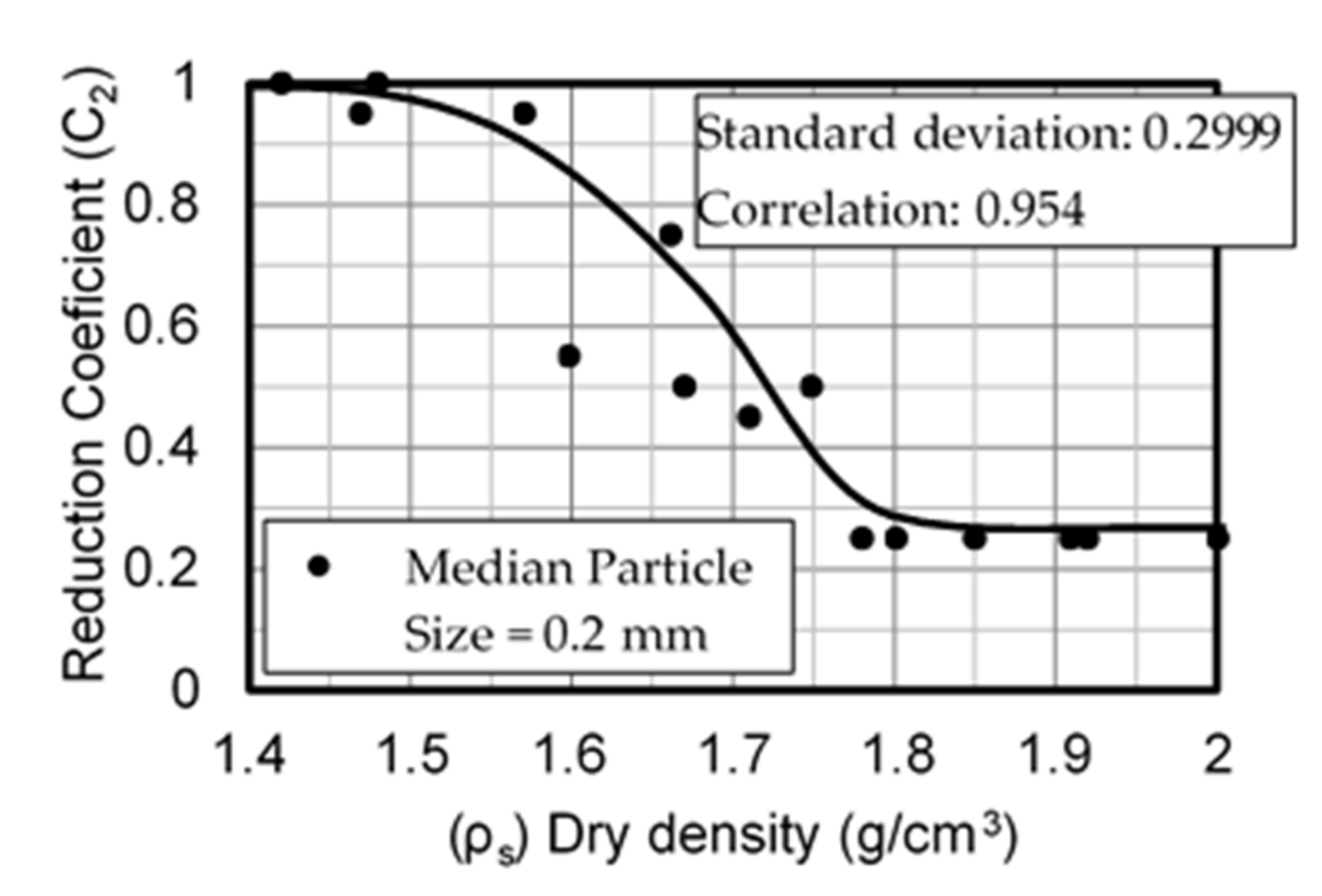
3.2. Rational Evaluation of the Coefficient of Bed-Load Transport Rate
To calculate the bed-load transportation, the model of Ca et al. [15] uses Equation (22) [17]. To use this equation, one needs to calculate the bedload transport coefficient value using the graphs provided in Figure 5, Figure 6 and Figure 7 as well as Equation (27). The presented graphs and illustrations of their production and use are detailed in [19].
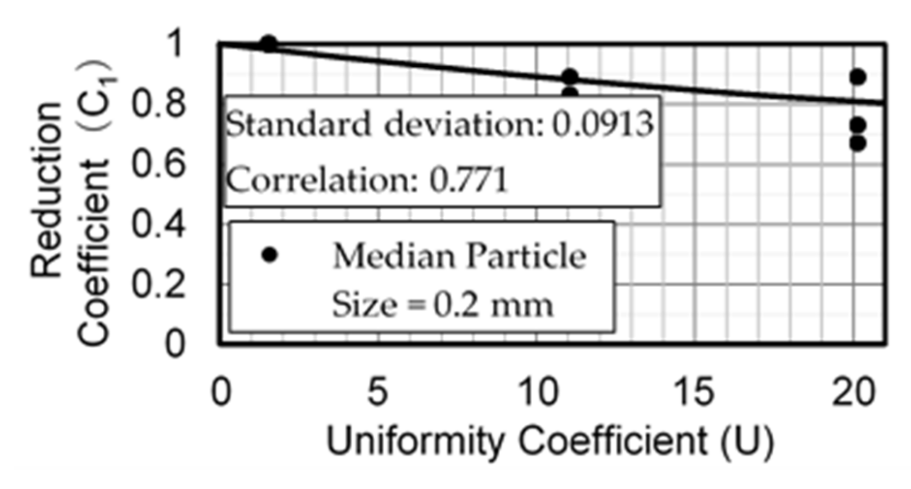
here, is bedload coefficient. It can be acquired from Figure 5 by knowing the median grain size, type of gravels (natural or crushed gravel) for a proposed area and assuming uniformity coefficient of 1.5~3, and dry density of around 1.5 g/cm3. and are reduction coefficients, can be acquired from Figure 6 and Figure 7 respectively.
4. Verification and Application of the Proposed Concept
For verification purposes, the famous Malpasset Dam’s hydrograph is generated using the proposed dam-break outflow rate Equation (4), and it is compared to the model of Aureli et al. [10]. For applicability purposes, the proposed outflow equation is integrated into an existing 2D long-wave flood simulation model of Ca et al. [15]. Even though there are several widely used flood simulation models such as MIKE11, ISIS, ONDA, FLU-COMP and HEC-RAS [26], or the recent and more advanced SPH approach models such as SPHERA [27], the authors have used the model of Ca et al. [15] because of having enough experience of using this model which has given consistent results. This model uses the two-dimensional non-linear shallow water equations, the continuity equation for hydrodynamics calculations and Rebberink’s equation [17] for modeling sediment transport. Since the data of a real dam-break are very difficult to achieve [28], and dam-break flood and a tsunami flood are almost similar [29], the validity of this model for a long wave flood routing was previously investigated by performing many tsunami simulations on the Sendai-Natori coast of Japan, which was hit by the Great East Japan Tsunami in 2011 [19].
4.1. Malpasset Dam-Break Hydrograph
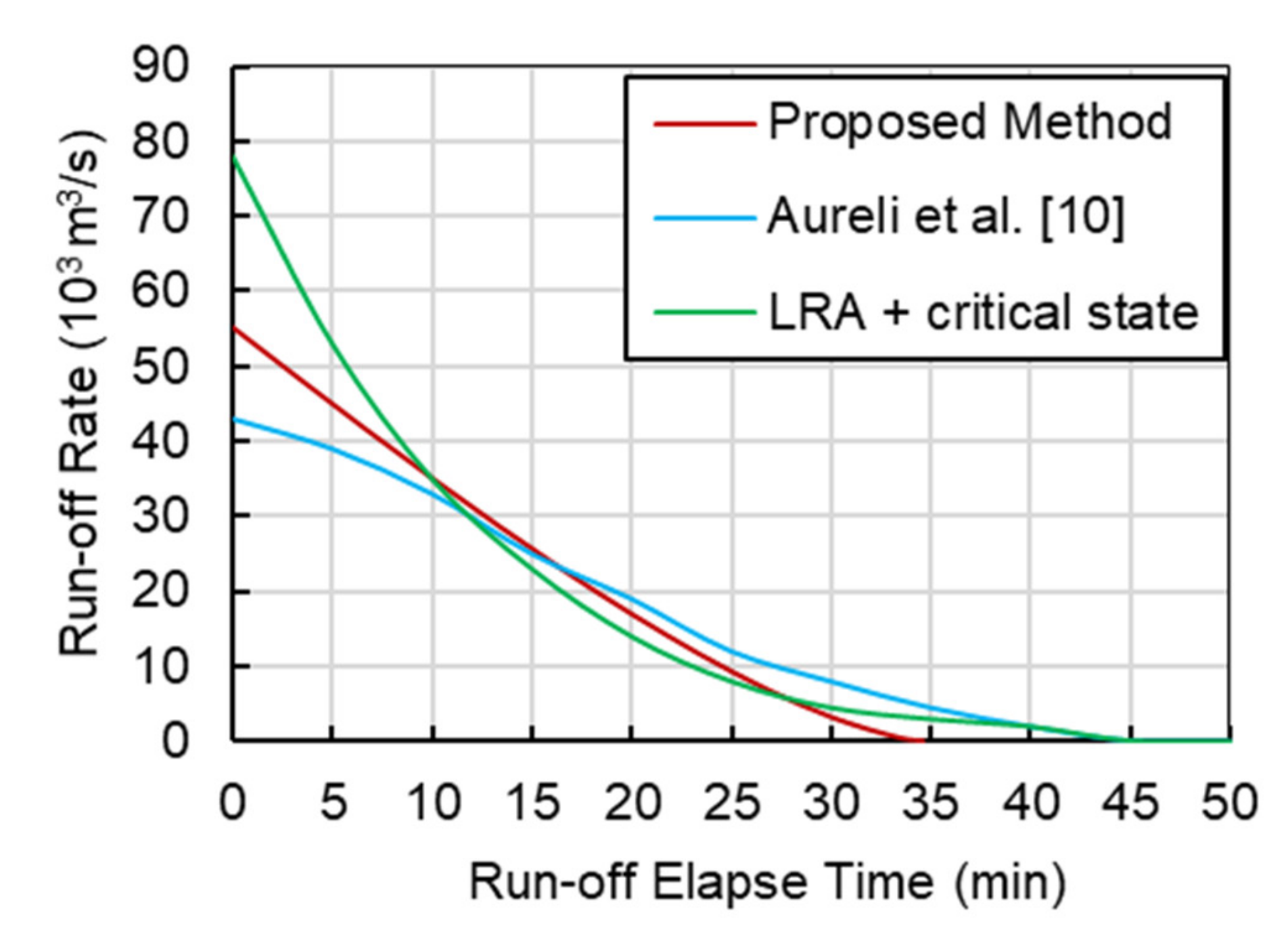
Malpasset Dam was a double-curvature arch-shaped structure located in the Frejus town of France. It had a crest length of approximately 223 m, a height of 66.5 m and a total reservoir capacity of 55 million cubic meters [30]. Following a flash flood on 2nd December 1959 at 21:14, the dam broke and a flood wave as tall as 40 m gushed through the valley towards the town of Frejus. Approximately 48 million cubics of water was released from the dam which caused the devastating catastrophe resulting in 433 casualties [30]. Due to the availability of measured flood propagation data from this dam break, it is quite popular in the literature and is often used as a case study for simulation verification [31,32,33]. Therefore, this paper intended to compare the Maspasset dam-break hydrograph generated using the newly proposed concept and the methods proposed by Aureli et al. [10]. For comparison purposes, the authors have set the break dimensions assuming a partial dam break. 85% of the crest length = 189.6 m as well as the same percentage of the dam height = 56.53 m is assumed broken which is more realistic than a full section dam-breaking assumption assumed by Aureli et al. [10]. Furthermore, the peak discharge flow rate from the proposed method is higher than the Aureli et al. [10] method and lower than the LRA method as shown in Figure 8. Moreover, the emptying time of the proposed method is the fastest among other methods. The reason behind these differences lies extensively in the different initial assumptions for developing these methods. For example, in the proposed method, the inference of reservoir bed slope, as well as water surface gradient during the emptying process, is neglected where this part can be improved in the future.
4.2. Hydro-Morphodynamics Simulation in Sendai-Natori Coast
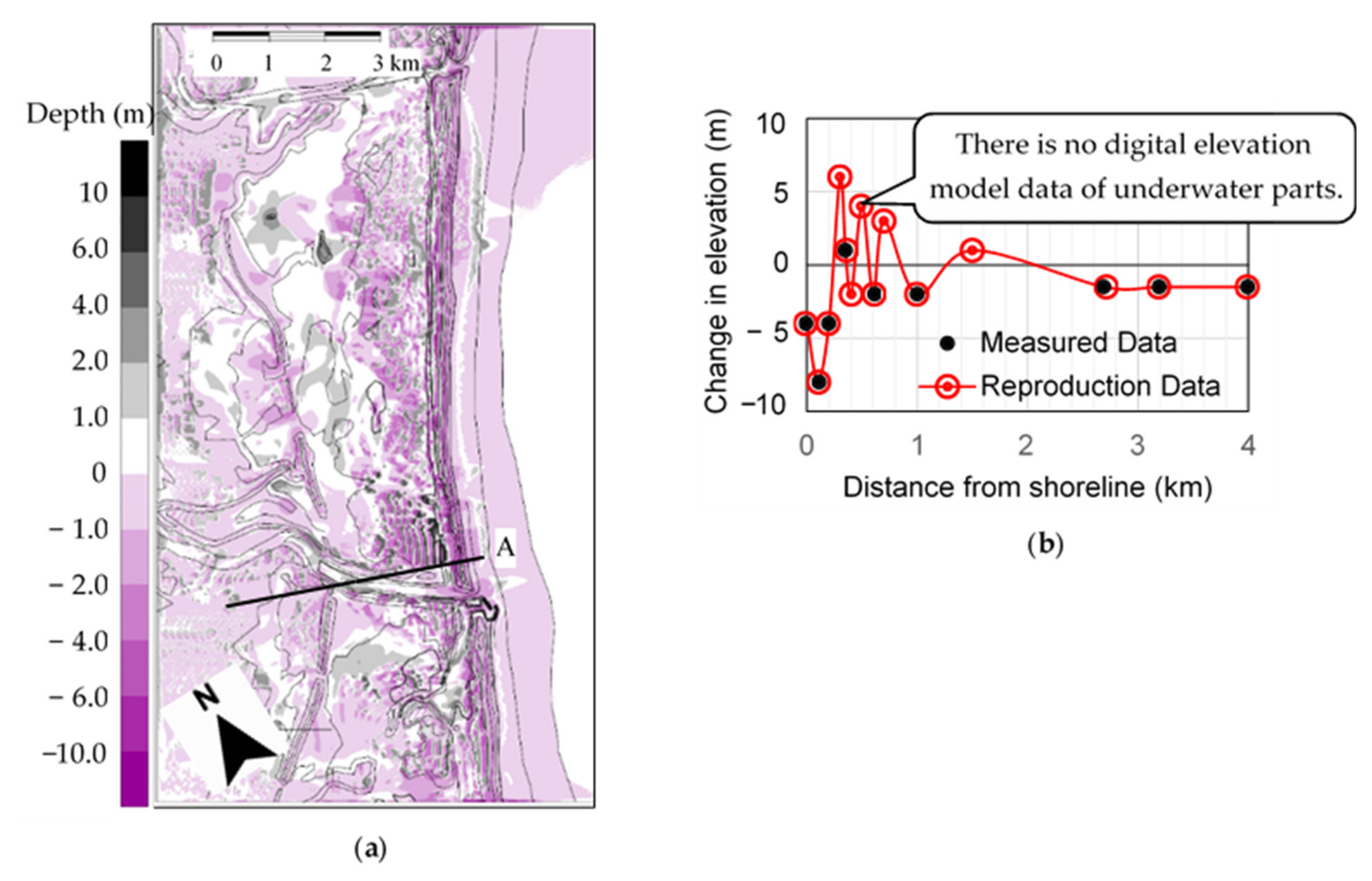
Sendai-Natori coast is located in the Miyagi prefecture of Japan. This coast experienced a magnitude 9.0 earthquake and a consequent catastrophic great tsunami in 2011. The authors executed many hydro-morphodynamics simulations to replicate the actual flooding conditions and presented the results on [19]. The authors also showed in their paper that the results of the simulations are in good agreement with the actual measured data from the area as shown in Figure 9b. Random spot elevation-change points are selected along the line (A) shown in Figure 9a, and their relative data are plotted from both measured data and the reproduction data. For the locations where measured data is available, the calculated data matches perfectly with the measured data. However, for some locations such as the seaside or underwater parts, because there is no digital elevation model data available, one cannot decide whether it differs from the actual topography change situation.
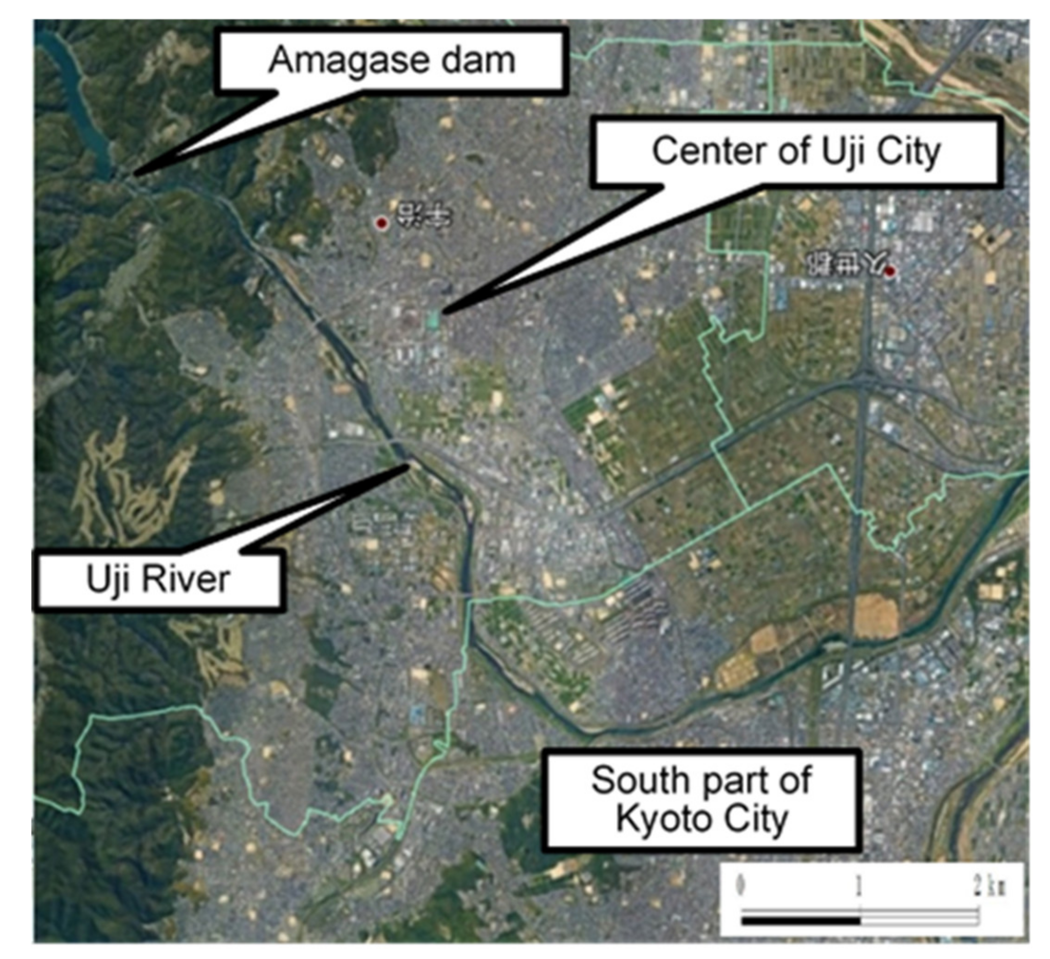
4.3. Dam-Break Hydro-Morphodynamics Simulation (Amagase Dam)
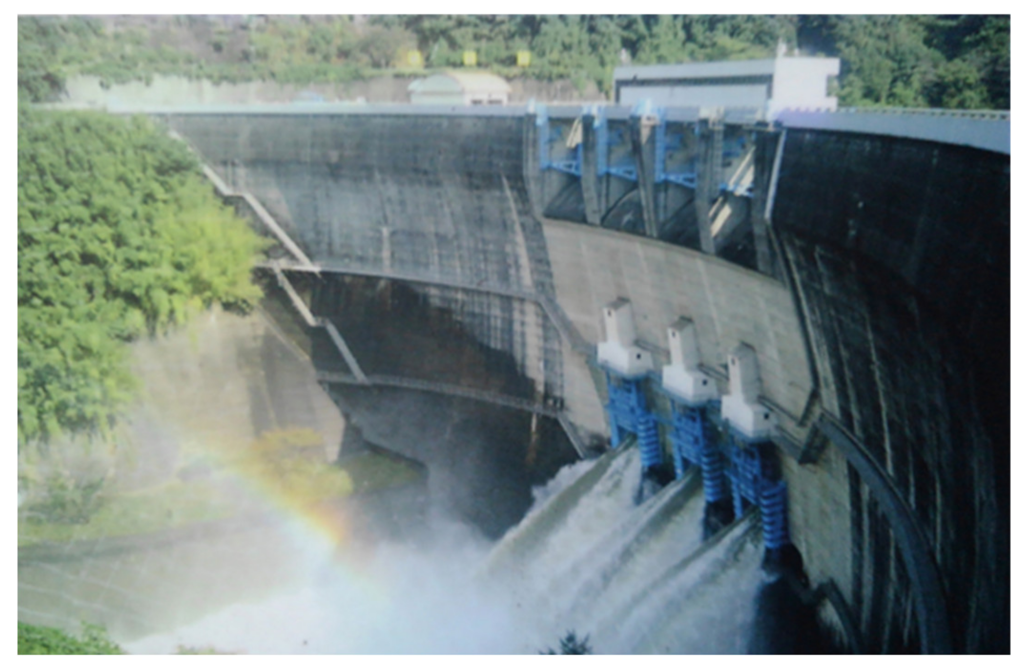
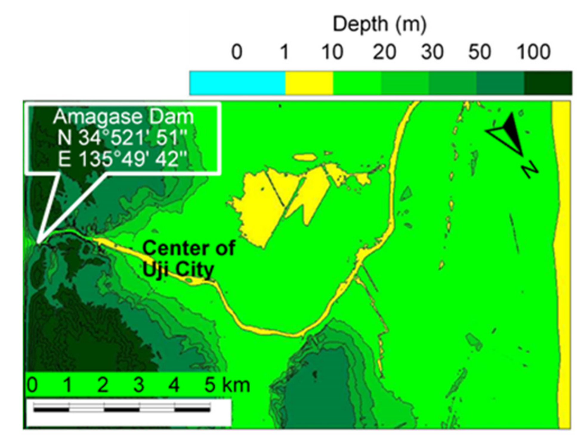
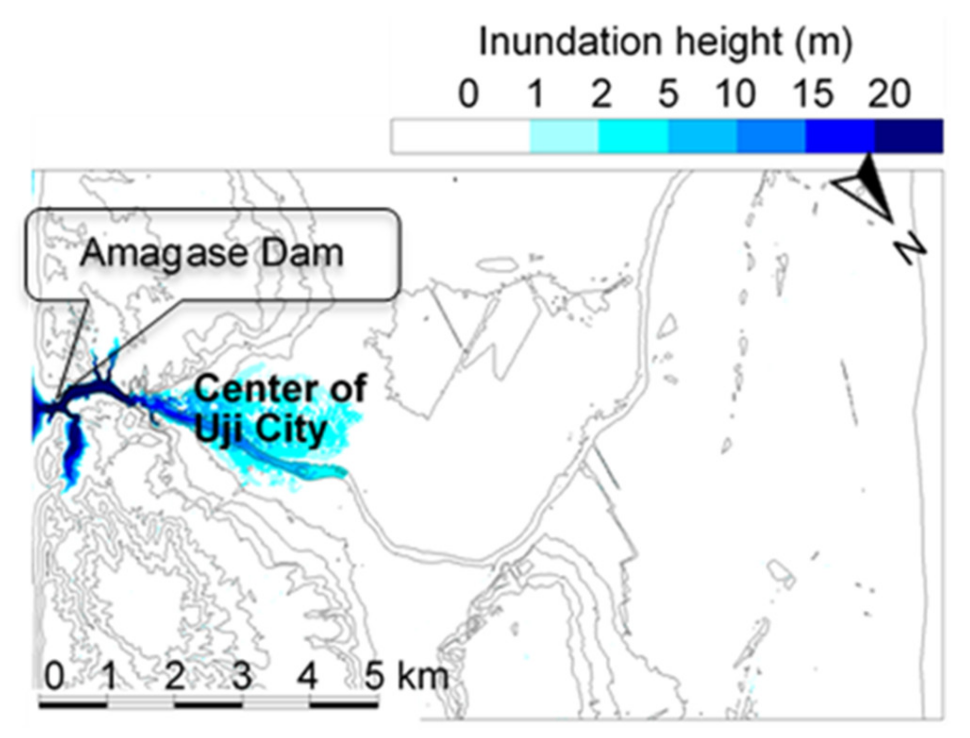
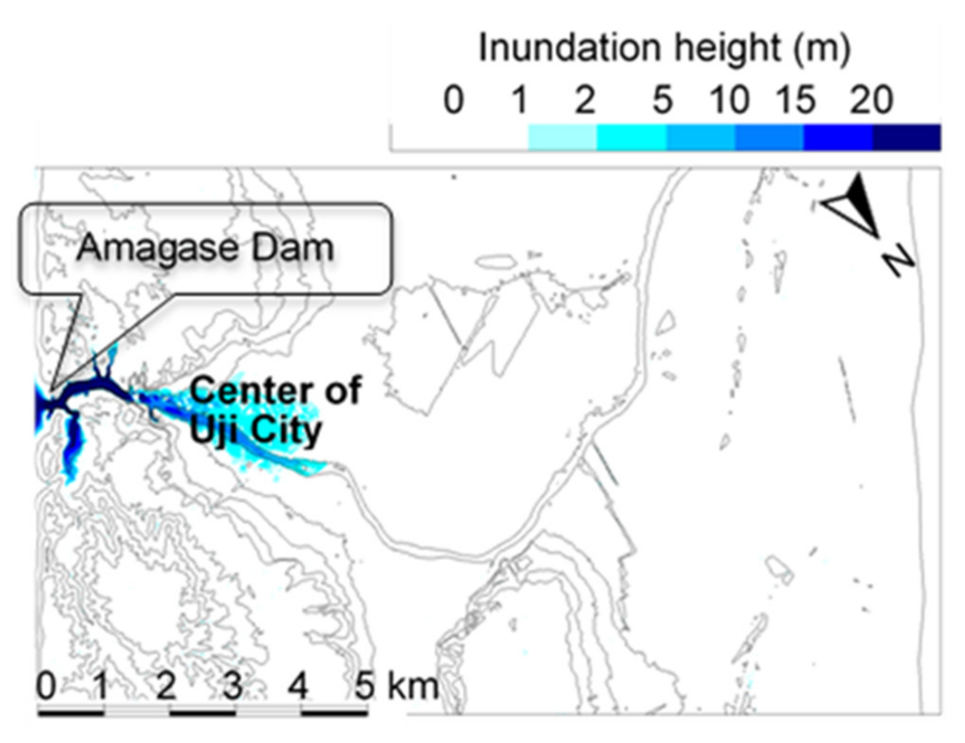
Amagase Dam is located in Uji City in Kyoto Prefecture of Japan. (Figure 10). It is an arch dam made of concrete, built on the Uji-Gawa river (Figure 11). The Amagase dam’s construction started in 1955 and finished in 1964. This dam is mainly constructed for flood control. It also serves as a great water supply reservoir for the Uji City residents. The catchment area of the dam is 4200 km2 and its design volume is 122 thousand cubic meters. The height of the dam is 73 m with a crest length of 254 m. The reason behind why this dam is chosen for simulation is, about 200 thousand people live downstream of the dam. If this dam breaks due to a mega earthquake or any other possible cause, it would be catastrophic. Therefore, in this paper, it is intended to prepare a hazard map to depict the inundation height, velocity, scouring and deposition depths for the possible affected area.
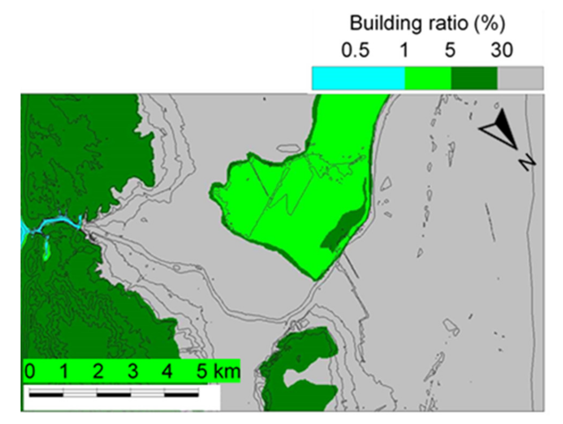
For the proposed dam-break simulation, the following information is required as input data sets; (1) assumed broken width and height, as listed in Table 2. (2) Proposed dam’s reservoir area, as listed in Table 2. (3) Water head behind the dam, as listed in Table 2. (4) Calculation meshes size, as listed in Table 2. Since the proposed model of Ca et al. [15] is based on the finite difference method (FDM), the mesh size limitation is always a concern which mainly depends on the capacity of the available computer, size of the proposed dam and required accuracy. (5) The existing topography contour map is shown in Figure 12. in this research, a 10-m accuracy digital elevation map (DEM) is used, (6) The building and trees ratio in a mesh (as shown in Figure 13, the light green color (the building ratio is 1 % in a mesh area) is referred to a soil and sand area, the dark green color (5 % in a mesh area) shows a wood area and a forest area, the light brown (30 % in a mesh area) shows a house with a garden, the gray color area (70 % in a mesh area) shows a building area, (7) Grain size distribution in the area and (8) Calculation limit boundary. (9) Acquiring the bedload roughness coefficient by using Figure 5, Figure 6 and Figure 7 and Equation (27). In the downstream of Amagase dam, from the position of topography change, there are three types of areas. (a) The high-altitude areas where the flood water cannot inundate. (b) The wetland area (Agricultura area) and (c) the city area.
For type (a) area, there is no need for bedload coefficient. For types (b and c), the calculations are detailed in the following.
For type (b) area:
- , using Figure 5,
- Uniformity coefficient, . Using Figure 6,
- Dry density . Using Figure 7,
- From Equation (27), .
For type (c) area:
- , using Figure 5,
- Uniformity coefficient, . Using Figure 6,
- Dry density . Using Figure 7,
- From Equation (27), .
The value of is set to 1000 m and the shape value is set to 0.28. the method and logic behind deciding the value is previously described in Section 3.1 of this paper.
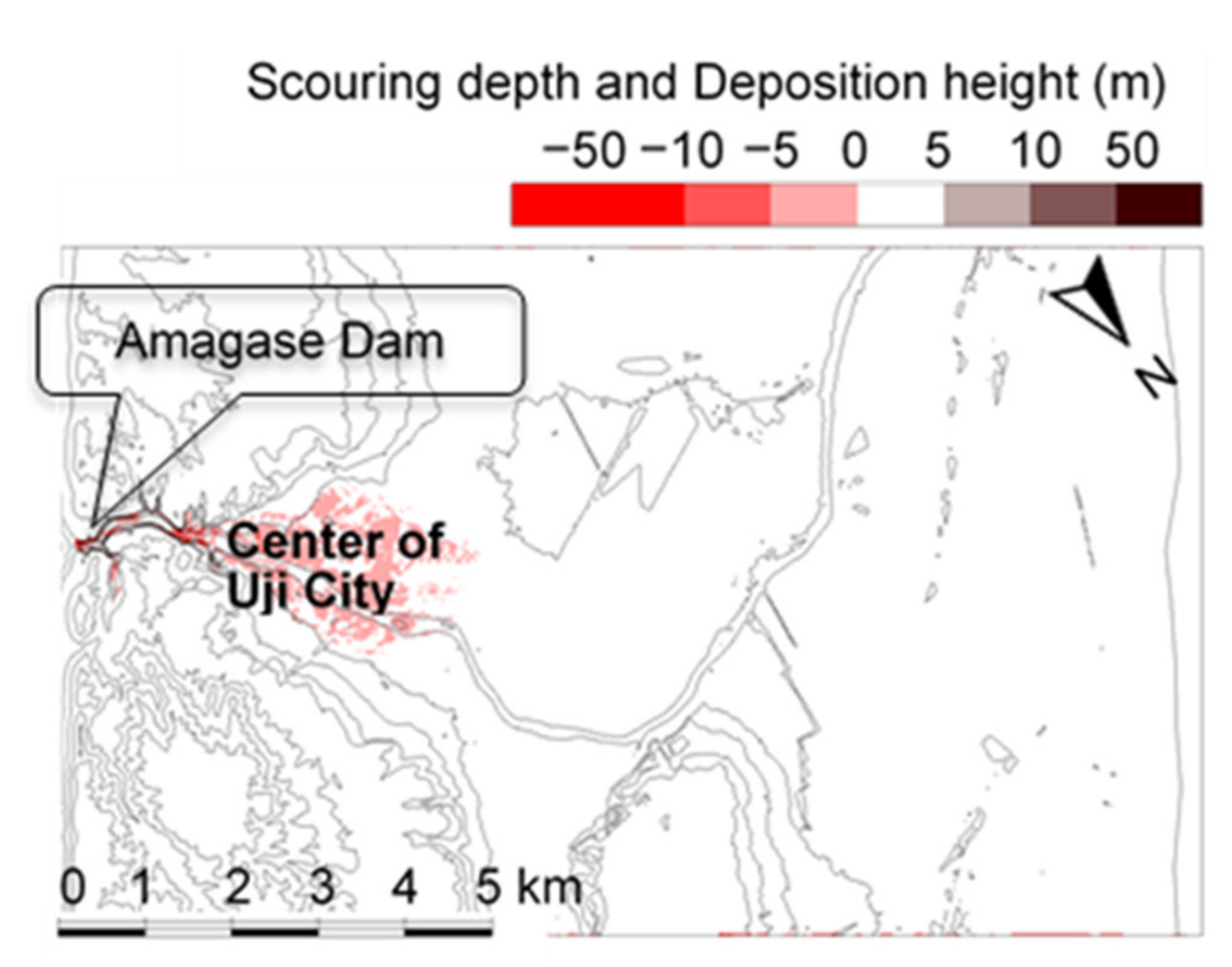
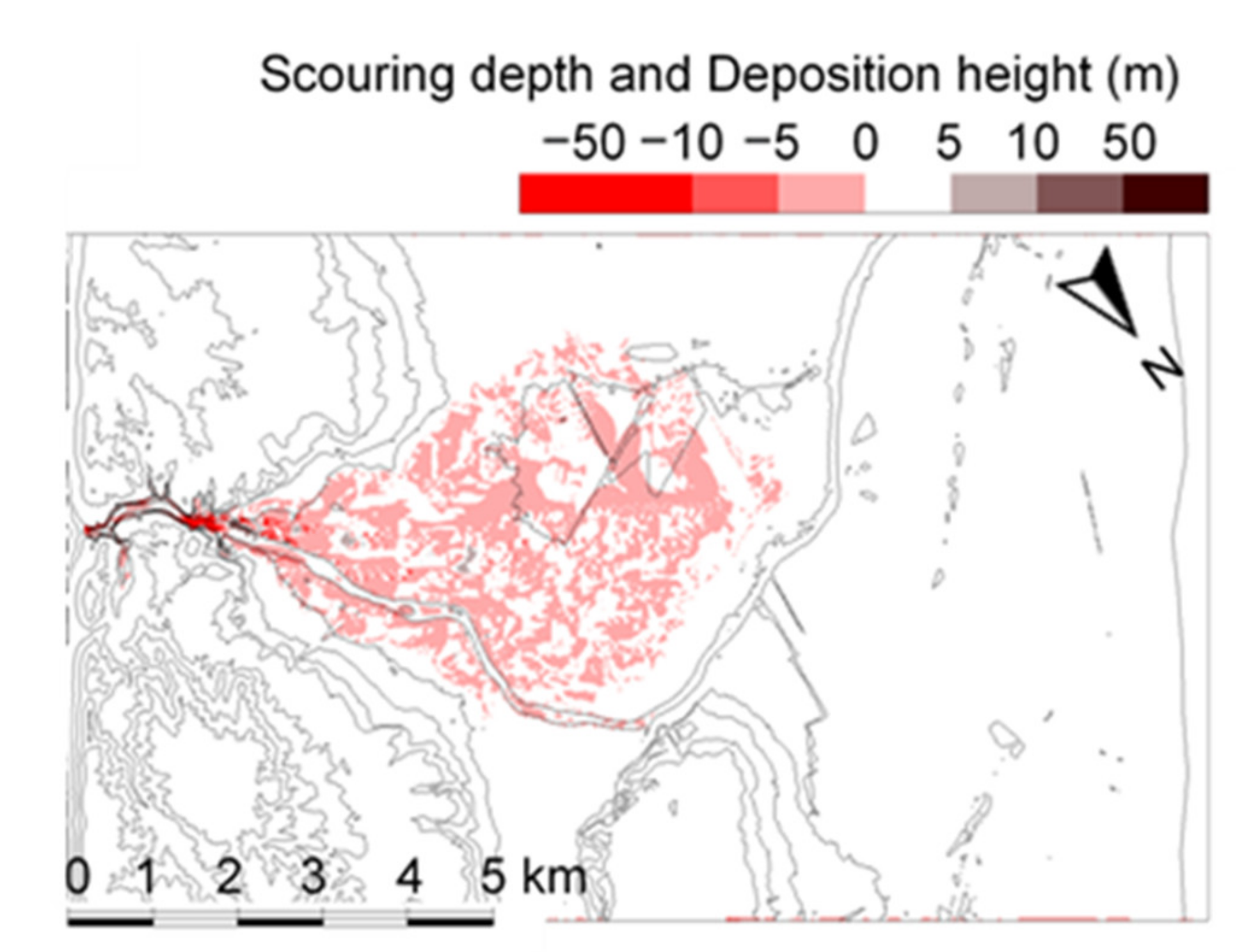
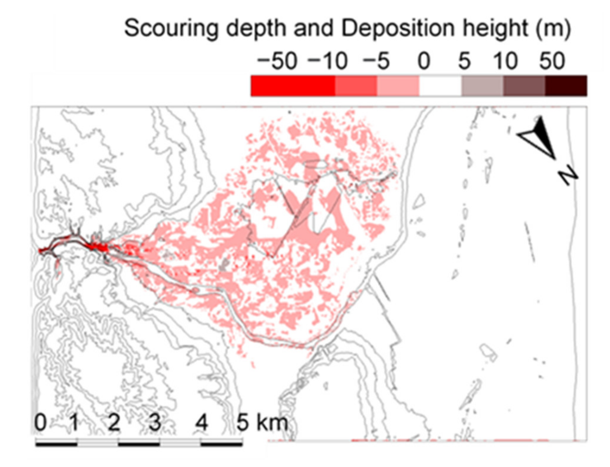
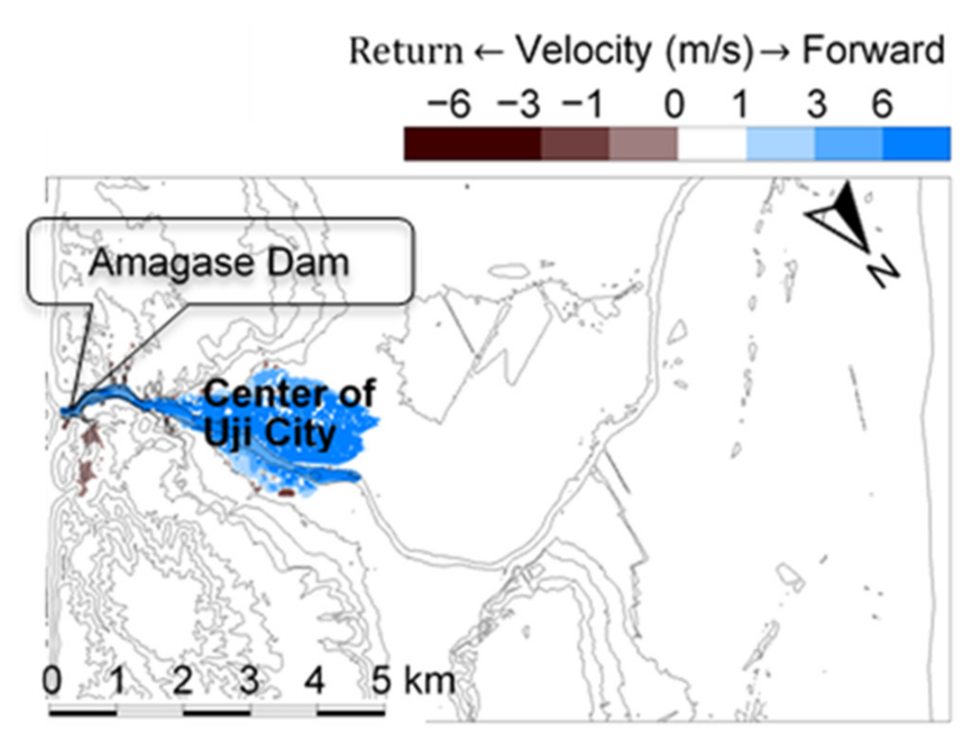
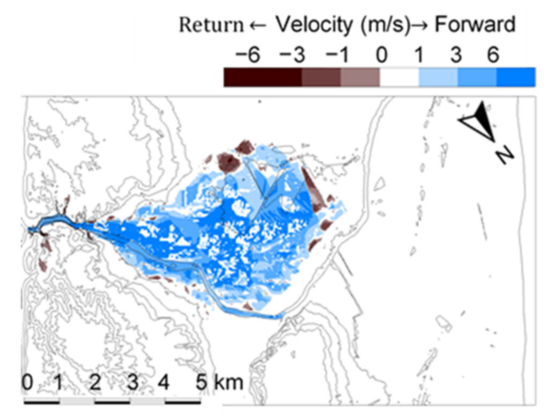
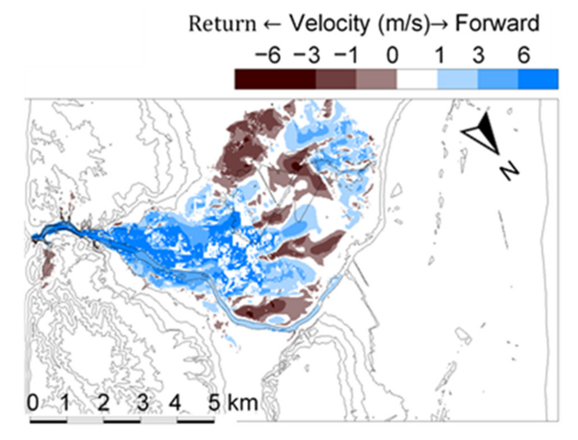
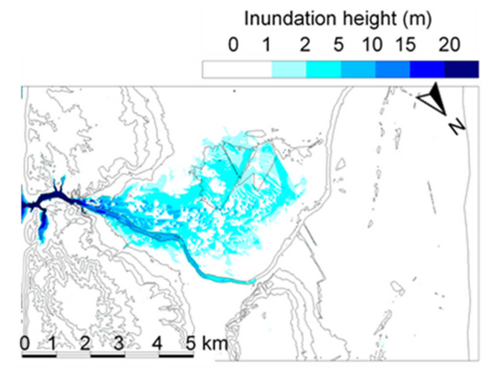
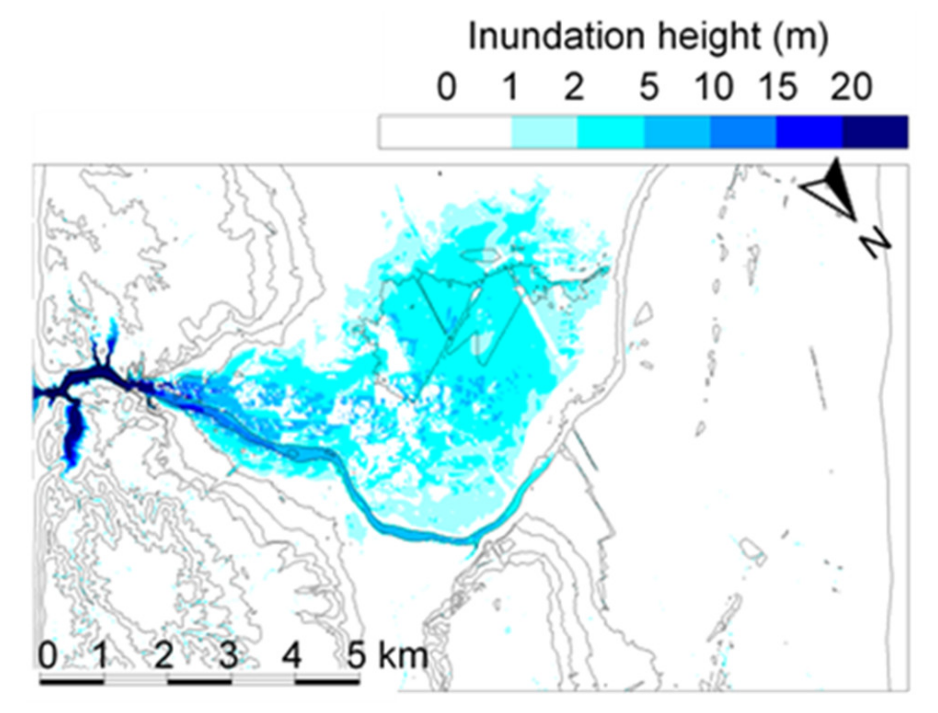
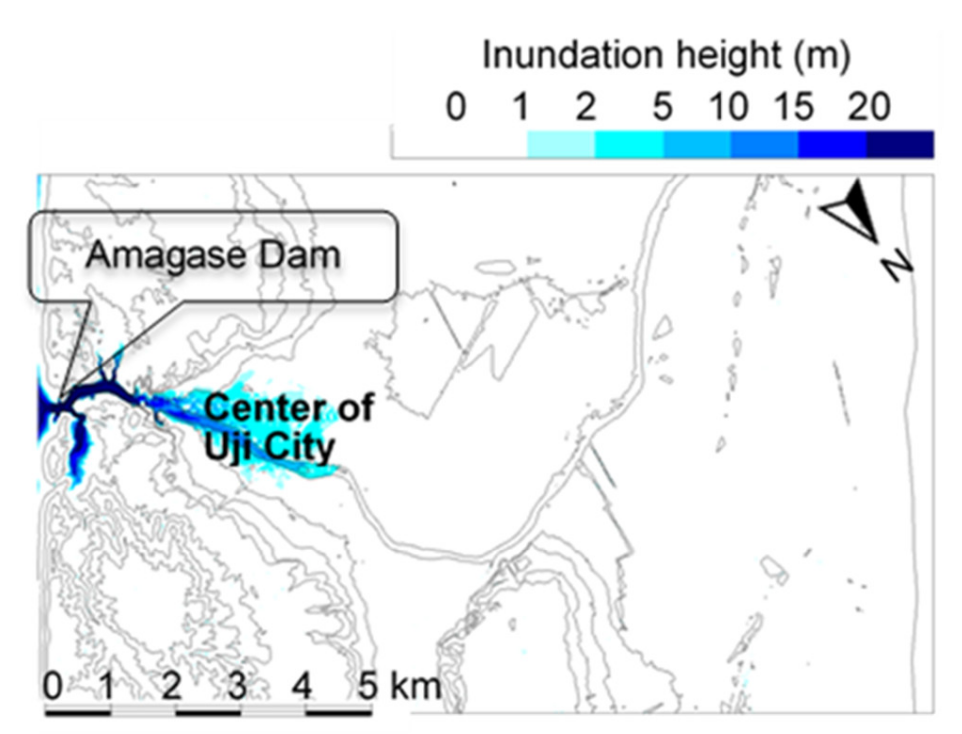
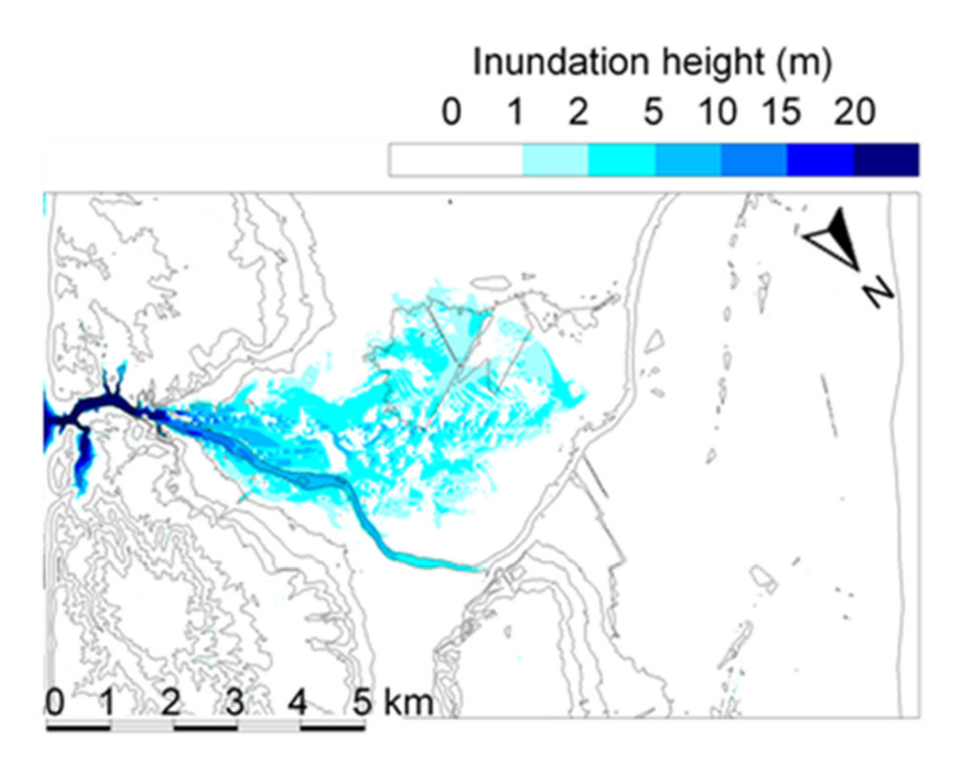
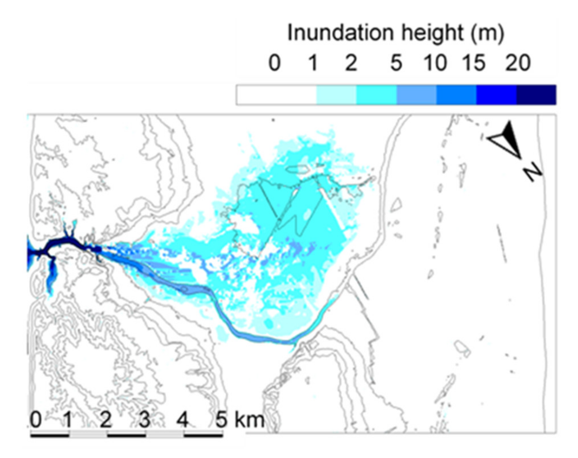
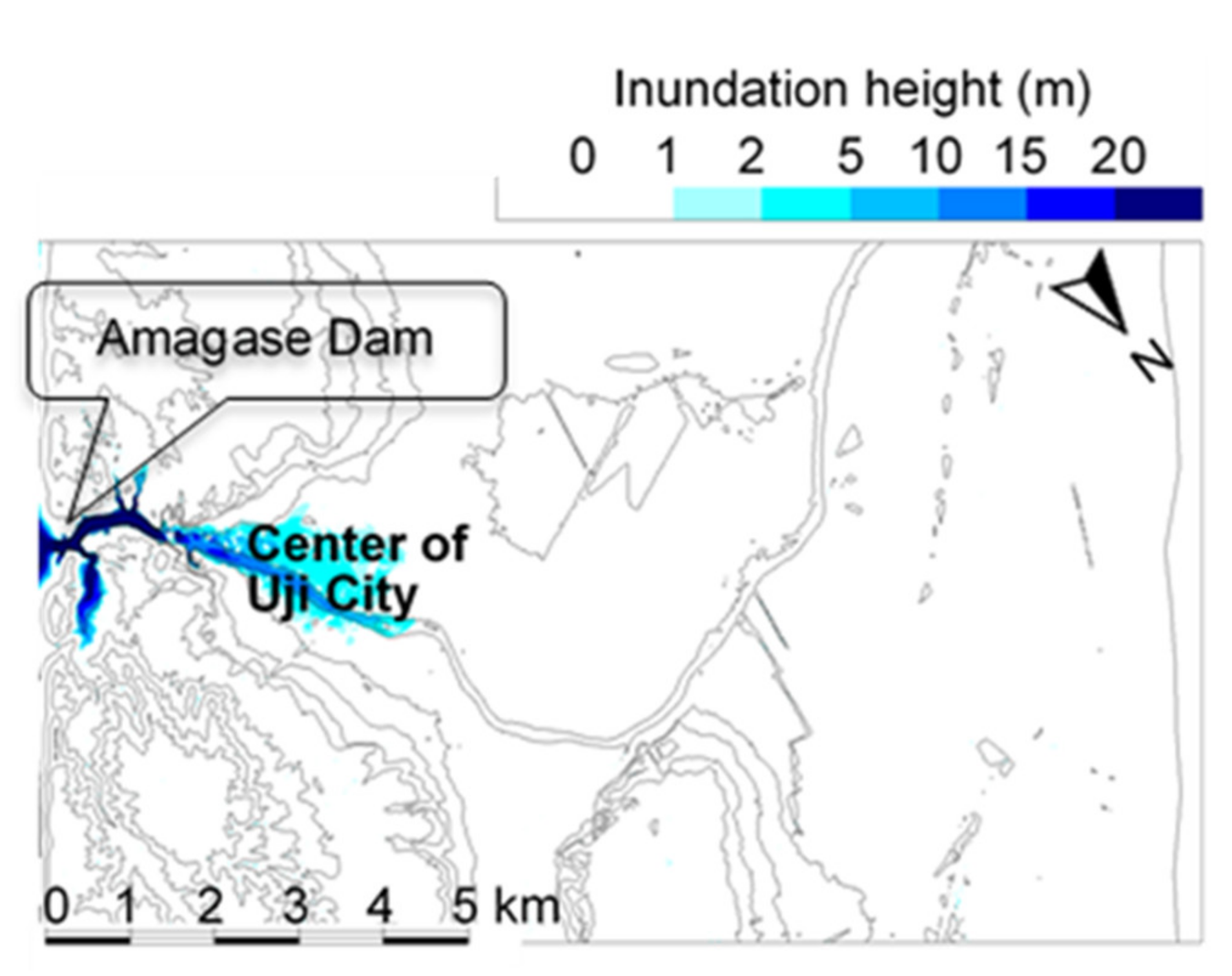
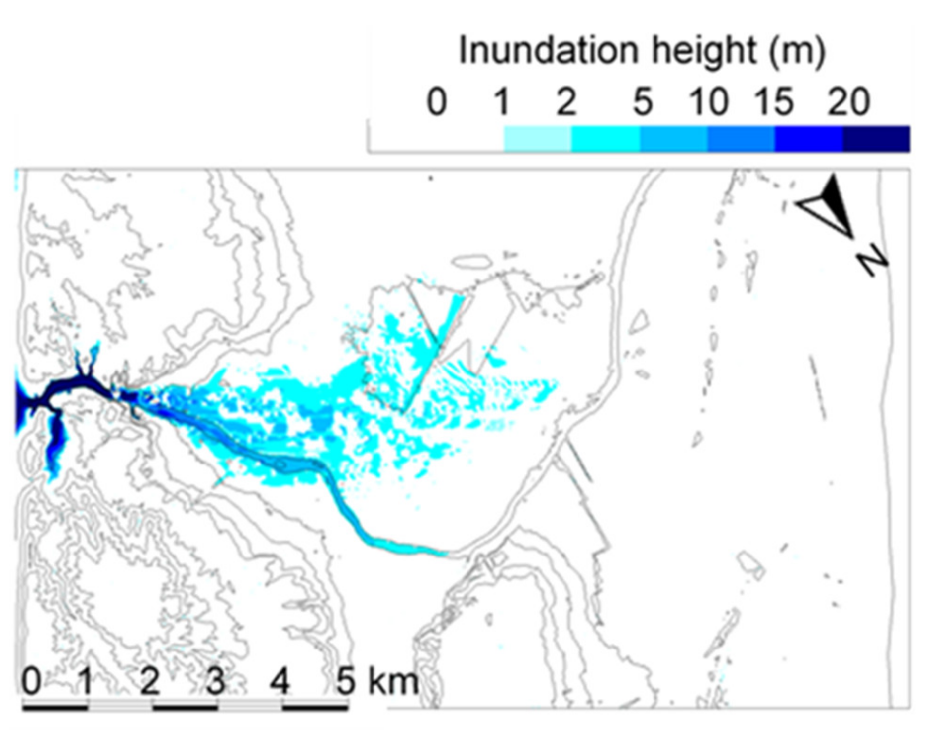
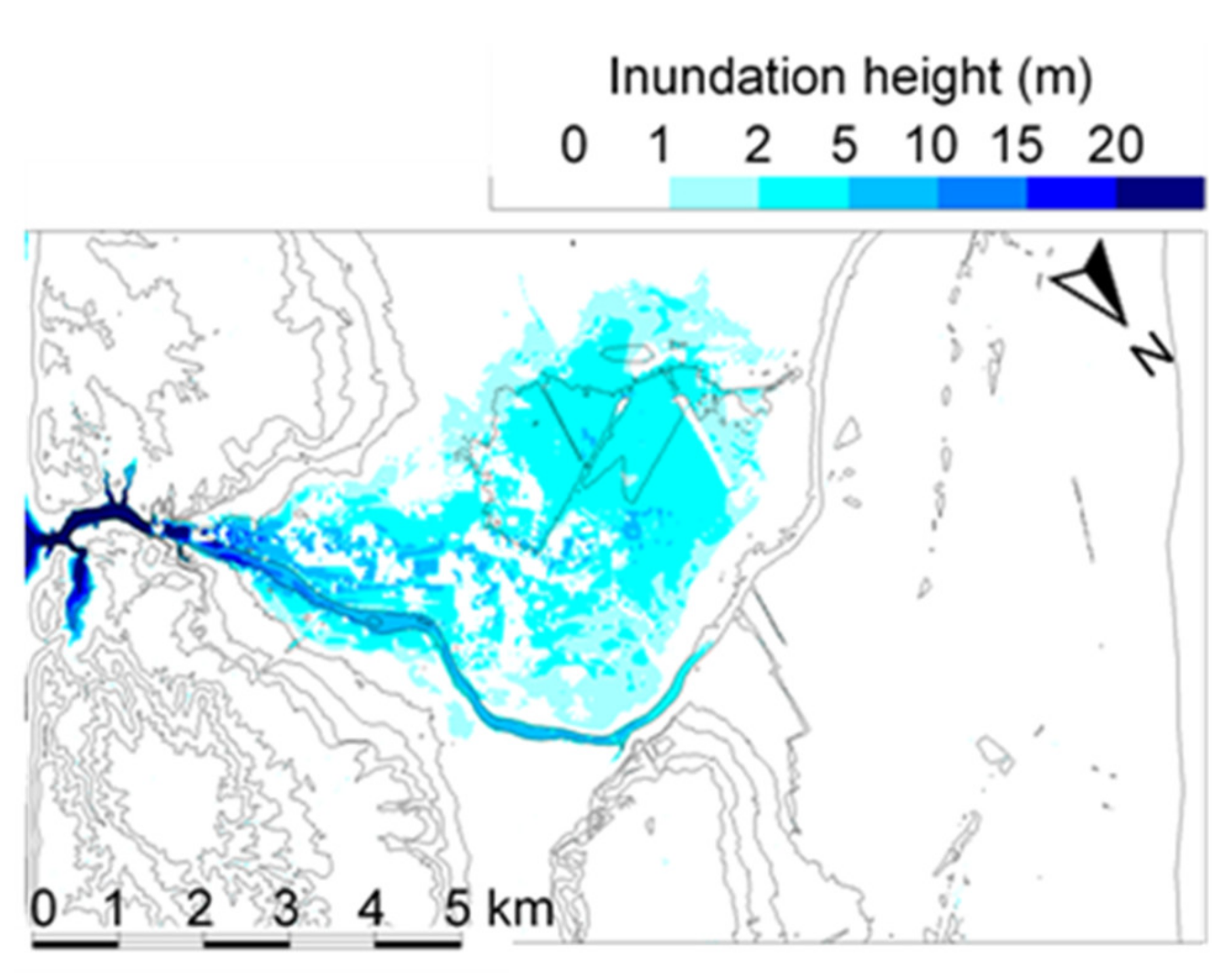
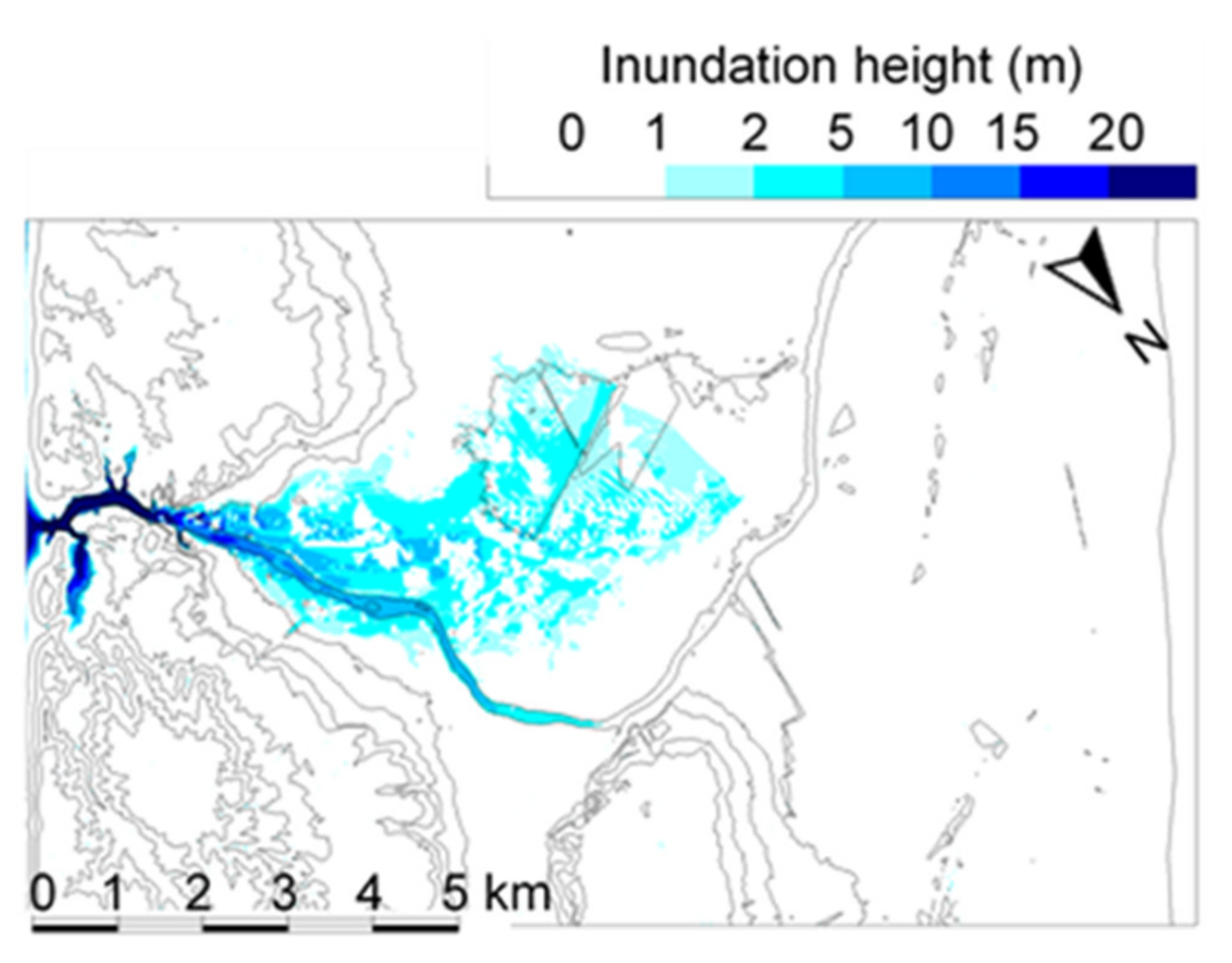
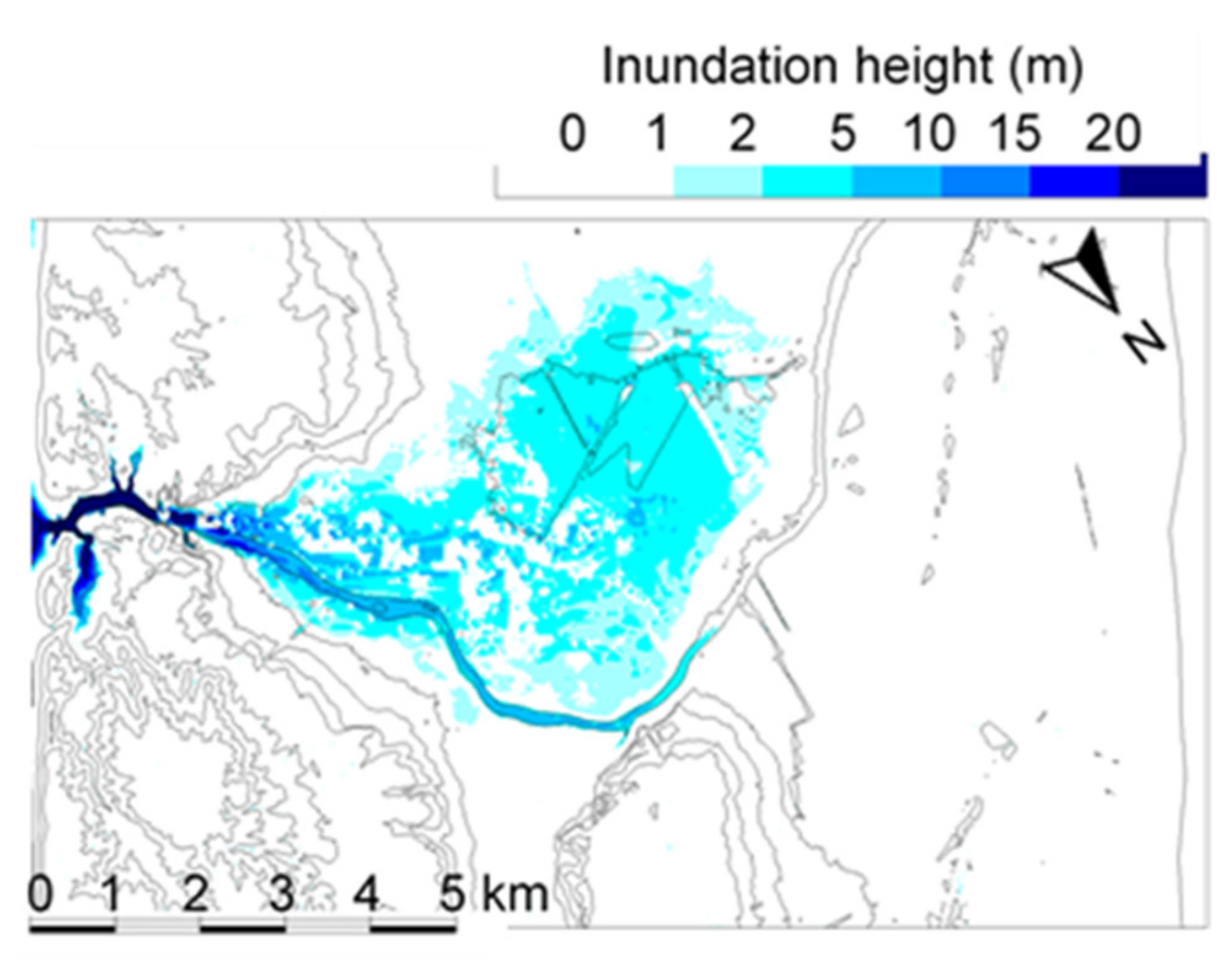
The results of the Amagase dam-break simulation are shown in Figure 14, Figure 15, Figure 16, Figure 17, Figure 18, Figure 19, Figure 20, Figure 21, Figure 22, Figure 23, Figure 24, Figure 25, Figure 26, Figure 27, Figure 28, Figure 29, Figure 30 and Figure 31. Scouring depths and deposition heights are depicted in Figure 14, Figure 15 and Figure 16. The maximum scouring depth is about 10 m close to the dam and it decreases to about 5 m as the bore reaches further locations from the dam. Forward and return velocity distributions are depicted in Figure 17, Figure 18 and Figure 19, the maximum forward velocity is calculated to be about 6 m per second and the maximum return velocity is found to be 3 m per second. Inundation height and extent are depicted in Figure 20, Figure 21 and Figure 22. Since the accurate dam-break section’s dimensions are difficult to anticipate, one needs to perform a dam-break with different possible break sections to find out the maximum inundation extent and velocity. Since a dam-break simulation takes time and effort, the authors in this paper executed many dam-break simulations with different heights and widths to evaluate and generalize the effect of a dam-break section’s height and width on the inundation area and velocity, as listed in Table 2. Four cases of break sections are assumed. The first case’s break section height is twice the height of the second case with the same width between the second case and the third case, the height is kept the same and the height of the third case is half of the second case. Between case four and the first case, again the height is kept the same however the width is half size. A brief comparison of the dam-break simulation results is depicted in Table 3.
Considering the width and height of different break sections (cases 1 through 4), the results of the simulations show that, as the height of the break section increases, the flood velocity and flood range becomes larger.
5. Conclusions
This study presented a novel, useful and simple approach for sudden partial dam break outflow rate. Using the proposed approach, one can assume different dam-break shapes and observe the relative generated hydrographs and decide the best condition to match a proposed dam for break simulation. The merits of the proposed approach are being simple to set up, minimum input values from a dam, such as dam height, width, reservoir surface area and an assumed dam-break section.
Naturally, in the case of non-erodible dams, the dam failure is usually a partial break. Therefore, the proposed equation was developed so that one can set a percentage failure of the dam and observe its hydrograph. The proposed equation is affected by the break section’s shape. Therefore, by performing many hydraulic experiments, a mean shape factor is acquired that can be set for different dam-break shapes. While executing the hydraulic experiments, it is observed that the water surface gradient is not level during the dam reservoir emptying process, therefore, the inference of water surface gradient on the proposed dam-break outflow rate concept, during a dam reservoir emptying process can be a potential future research objective.
Furthermore, to show the validity of the proposed equation, the Malpasset dam-break hydrograph is produced and compared to that of the existing literature. In this comparison, the proposed equation resulted in a relatively higher peak discharge and faster emptying time and it is concluded that the reason behind this is the different initial conditions for developing the different equations. The reliability of the proposed equation and the existing equations in the literature is the same. However, the proposed equation is easy to set up and one can simply evaluate the inference of different dam-break sections on a dam-break outflow rate.
Consequently, by integrating the proposed outflow rate equation on a two-dimensional flood simulation model, and simulating the Amagase dam-break, it is perceived that this equation can be potentially useful for the preparation of dam-break flood routing. According to the simulation results of the Amagase Dam presented in this paper, thousands of lives, as well as a countless amount of economy/businesses, are in a high-risk zone in the case of a dam break. Therefore, the authors suggest that when the dam becomes old, because it will be less durable against a great earthquake, the households living downstream of the dam and in the high-risk zone should be informed of the potential danger; i.e., in the case of superannuated dams in the area where the frequency of Mega Earthquakes is high, the preparation of hazard maps, emergency action plans and early warning systems will be very useful and will lead to the saving of lives and the economy. Especially in the case of the Amagase dam, which a densely populated city is located right at its downstream, widening the dam would result in lowering its risk of calamity in case of a dam-break.
Author Contributions
Conceptualization, S.M.A. and Y.Y.; methodology, S.M.A. and Y.Y.; software, S.M.A.; validation, S.M.A.; formal analysis, S.M.A. and Y.Y.; investigation, S.M.A. and Y.Y.; resources, Y.Y.; data curation, S.M.A.; writing—original draft preparation, S.M.A.; writing—review and editing, S.M.A. and Y.Y.; visualization, S.M.A.; supervision, Y.Y.; project administration, Y.Y.; funding acquisition, S.M.A. and Y.Y. All authors have read and agreed to the published version of the manuscript.
Funding
This research was partially funded by Japan Society for the Promotion of Science grant number 18k04667. And the APC was funded by Ministry of Education, Culture, Sports, Science and Technolog—Japan.
Institutional Review Board Statement
Not applicable.
Informed Consent Statement
Not applicable.
Data Availability Statement
The data presented in this study are available on request from the corresponding author. The data are not publicly available due to privacy reasons.
Acknowledgments
This research was executed under the partial support of Grants-in-Aid for Scientific Research (c; 18k04667) of Japan Society for the Promotion of Science (JSPS). Here, we express gratitude deeply.
Conflicts of Interest
The authors declare no conflict of interest.
References
- Psomiadis, E.; Tomanis, L.; Kavvadias, A.; Soulis, K.X.; Charizopoulos, N.; Michas, S. Potential Dam Breach Analysis and Flood Wave Risk Assessment Using HEC-RAS and Remote Sensing Data: A Multicriteria Approach. Water 2021, 13, 364. [Google Scholar] [CrossRef]
- Wahl, T.L. Predicting Embankment Dam Breach Parameters—A Needs Assessment. In Proceedings of the XXVIIth IAHR Congress, San Francisco, CA, USA, 10–15 August 1997. [Google Scholar]
- Pilotti, M.; Tomirotti, M.; Valerio, G.; Bacchi, B. Simplified Method for the Characterization of the Hydrograph following a Sudden Partial Dam Break. J. Hydraul. Eng. 2010, 136, 693–704. [Google Scholar] [CrossRef]
- Costa, J.E. Floods from Dam Failures; Open-File Report; U.S. Geological Survey: Denver, CO, USA, 1985. [Google Scholar]
- Gary, G. Using HEC-RAS for Dam Break Studies; US Army Corps of Engineers: Washington, DC, USA, 2014. [Google Scholar]
- Wurbs, R.A. Dam-Breach Flood Wave Models. J. Hydraul. Eng. 1987, 113, 29–46. [Google Scholar] [CrossRef]
- Bazin, H. Recherches Expérimentales relatives aux remous et à la propagation des ondes [Experimental research on the hydraulic jump and on wave propagation]. Deux. Partie Rech. Hydraul. Darcy Baz. Dunod Paris 1865, 2, 148. [Google Scholar]
- Ritter, A. Die Fortpflanzung der Wasserwellen. [The propagation of water waves]. Z. Ver. Dtsch. Ing. 1892, 3633, 947–954. [Google Scholar]
- Su, S.-T.; Barnes, A.H. Geometric and Frictional Effects on Sudden Releases. J. Hydraul. Div. 1970, 96, 2185–2200. [Google Scholar] [CrossRef]
- Aureli, F.; Maranzoni, A.; Mignosa, P. A semi-analytical method for predicting the outflow hydrograph due to dam-break in natural valleys. Adv. Water Resour. 2013, 63, 38–44. [Google Scholar] [CrossRef]
- Saberi, O.; Zenz, G. Empirical Relationship for Calculate Outflow Hydrograph of Embankment Dam Failure due to Overtopping Flow. Int. J. Hydraul. Eng. 2015, 4, 45–53. [Google Scholar]
- Basheer, T.A.; Wayayok, A.; Yusuf, B.; Kamal, R. Dam breach parameters and their influence on flood hydrographs for mosul dam. J. Eng. Sci. Technol. 2017, 12, 14. [Google Scholar]
- Hakimzadeh, H.; Nourani, V.; Amini, A.B. Genetic Programming Simulation of Dam Breach Hydrograph and Peak Outflow Discharge. J. Hydrol. Eng. 2014, 19, 757–768. [Google Scholar] [CrossRef]
- Wahl, T.L. Prediction of Embankment Dam Breach Parameters—A Literature Review and Needs Assessment; Dam Safety Office: Denver, CO, USA, 1998. [Google Scholar]
- Ca, V.T.; Yamamoto, Y.; Charusrojthanadech, N. Improvement of Prediction Methods of Coastal Scour and Erosion due to Tsunami Back-flow. In Proceedings of the International Society of Offshore and Polar Engineers (ISOPE), Beijing, China, 20 June 2010. ISOPE-I-10-510. [Google Scholar]
- Suetsugi, T.; Kuriki, M. Research on Application for Flood Disaster Prevention and Simulation of Flooding Flow by Means of New Flood Simulation Model. Doboku Gakkai Ronbunshu 1998, 593, 41–50. [Google Scholar] [CrossRef] [Green Version]
- Ribberink, J.S. Bed-load transport for steady flows and unsteady oscillatory flows. Coast. Eng. 1998, 34, 59–82. [Google Scholar] [CrossRef]
- Yokoyama, Y.; Tanabe, H.; Torii, K.; Kato, F.; Yamamoto, Y.; Vu, T.C.; Arimura, J. A quantitative evaluation of scour depth near coastal structures. In Proceedings of the Coastal Engineering 2002; World Scientific Publishing Company: Cardiff, UK, 2003; pp. 1830–1841. [Google Scholar]
- Ahmadi, S.M.; Yamamoto, Y.; Ca, V.T. Rational Evaluation Methods of Topographical Change and Building Destruction in the Inundation Area by a Huge Tsunami. J. Mar. Sci. Eng. 2020, 8, 762. [Google Scholar] [CrossRef]
- Van Rijn, L.C. Principles of Sediment Transport in Rivers, Estuaries and Coastal Seas. 1: Principles of Sediment Transport in Rivers, Estuaries and Coastal Seas; Aqua Publications: Amsterdam, The Netherlands, 1993; ISBN 978-90-800356-2-1. [Google Scholar]
- Van Rijn, L.C. Sediment Transport, Part I: Bed Load Transport. J. Hydraul. Eng. 1984, 110, 1431–1456. [Google Scholar] [CrossRef] [Green Version]
- Van Rijn, L.C. Sediment Transport, Part II: Suspended Load Transport. J. Hydraul. Eng. 1984, 110, 1613–1641. [Google Scholar] [CrossRef]
- Van Rijn, L.C. Sediment Transport, Part III: Bed forms and Alluvial Roughness. J. Hydraul. Eng. 1984, 110, 1733–1754. [Google Scholar] [CrossRef]
- Richard Soulsby Dynamics of Marine Sands; Thomas Telford Ltd: London, UK, 1997; ISBN 978-0-7277-2584-4.
- Zyserman, J.A.; Fredsøe, J. Data Analysis of Bed Concentration of Suspended Sediment. J. Hydraul. Eng. 1994, 120, 1021–1042. [Google Scholar] [CrossRef]
- Bates, P.D.; De Roo, A.P.J. A simple raster-based model for flood inundation simulation. J. Hydrol. 2000, 236, 54–77. [Google Scholar] [CrossRef]
- Amicarelli, A.; Manenti, S.; Albano, R.; Agate, G.; Paggi, M.; Longoni, L.; Mirauda, D.; Ziane, L.; Viccione, G.; Todeschini, S.; et al. SPHERA v.9.0.0: A Computational Fluid Dynamics research code, based on the Smoothed Particle Hydrodynamics mesh-less method. Comput. Phys. Commun. 2020, 250, 107157. [Google Scholar] [CrossRef]
- He, G.; Chai, J.; Qin, Y.; Xu, Z.; Li, S. Evaluation of Dam Break Social Impact Assessments Based on an Improved Variable Fuzzy Set Model. Water 2020, 12, 970. [Google Scholar] [CrossRef] [Green Version]
- Kocaman, S.; Dal, K. A New Experimental Study and SPH Comparison for the Sequential Dam-Break Problem. J. Mar. Sci. Eng. 2020, 8, 905. [Google Scholar] [CrossRef]
- Goutal, N. The Malpasset dam failure. An overview and test case definition. In Proceedings of the 4th CADAM Meeting, Zaragoza, Spain, 18–19 November 1999; pp. 18–19. [Google Scholar]
- Alcrudo, F.; Gil, F. The Malpasset dam break case study. In Proceedings of the 4th CADAM Meeting, Zaragoza, Spain, 18–19 November 1999; pp. 18–19. [Google Scholar]
- Hervouet, J.-M.; Petitjean, A. Malpasset dam-break revisited with two-dimensional computations. J. Hydraul. Res. 1999, 37, 777–788. [Google Scholar] [CrossRef]
- Valiani, A.; Caleffi, V.; Zanni, A. Case Study: Malpasset Dam-Break Simulation using a Two-Dimensional Finite Volume Method. J. Hydraul. Eng. 2002, 128, 460–472. [Google Scholar] [CrossRef]
Figure 1.
Dam-break plan (a) and section view (b).

Figure 2.
Explanation of and in a control volume. The shaded area shows wet portion. The gray area shows dry portion.
Figure 2.
Explanation of and in a control volume. The shaded area shows wet portion. The gray area shows dry portion.

Figure 3.
(a) Dam-break experiment apparatus. (b) Dam-break experiment in a rectangular channel.

Figure 4.
(Case 1–4) Dam-break hydrographs from experimental cases and calculated using Equation (4).
Figure 4.
(Case 1–4) Dam-break hydrographs from experimental cases and calculated using Equation (4).

Figure 5.
Influence of the median grain size to the bed-load coefficient (Uniformity coefficients are 1.5~3, dry densities are around 1.5 g/cm3).
Figure 5.
Influence of the median grain size to the bed-load coefficient (Uniformity coefficients are 1.5~3, dry densities are around 1.5 g/cm3).

Figure 6.
Influence of the uniformity coefficient to the bed-load reduction coefficient (the median grain size is 0.2 mm; dry densities are around 1.5 g/cm3).
Figure 6.
Influence of the uniformity coefficient to the bed-load reduction coefficient (the median grain size is 0.2 mm; dry densities are around 1.5 g/cm3).

Figure 7.
Influence of dry density to the bed-load reduction coefficient (the median grain size and the uniformity coefficient are 0.2 mm and 20.1).
Figure 7.
Influence of dry density to the bed-load reduction coefficient (the median grain size and the uniformity coefficient are 0.2 mm and 20.1).

Figure 8.
The Malpasset dam hydrograph comparison between the proposed method of this paper, method of Aureli et al. [10] and Level Reservoir Approximation together with the imposition of the critical state at the dam site during the emptying process, Aureli et al. [10].

Figure 9.
(a) Topography change results (Total bed—load), 48 min from start of the tsunami calculations [19]. (b) Relative accuracy of the topography-change along line (A)—shown on Figure 9. (a)—on the measured and reproduced simulation results [19].

Figure 10.
Locations of Amagase Dam and the high-density zone of the population of Uji City (the gray zone is the circumference of “Center of Uji City”).
Figure 10.
Locations of Amagase Dam and the high-density zone of the population of Uji City (the gray zone is the circumference of “Center of Uji City”).

Figure 11.
A photo of Amagase Dam (the dam height is 73 m, the dam width is 254 m).

Figure 12.
Existing topography—Downstream of Amagase dam (Uji City).

Figure 13.
Building ratio in a calculation mesh (=the area ratio of buildings and trees in a mesh).

Figure 14.
(Case–1). Topography change, 10 min after the start of the calculation.

Figure 15.
(Case–1). Topography change, 20 min after the start of the calculation.

Figure 16.
(Case–1). Topography change, 30 min after the start of the calculation.

Figure 17.
(Case–1). Inundation velocity, 10 min after the start of the calculation.

Figure 18.
(Case–1). Inundation velocity 20 min after the start of the calculation.

Figure 19.
(Case–1). Inundation velocity 30 min after the start of the calculation.

Figure 20.
(Case–1). Inundation height, 10 min after start of the calculation.

Figure 21.
(Case–1). Inundation height, 20 min after start of the calculation.

Figure 22.
(Case–1). Inundation height, 30 min after start of the calculation.

Figure 23.
(Case–2). Inundation height, 10 min after start of the calculation.

Figure 24.
(Case–2). Inundation height, 20 min after start of the calculation.

Figure 25.
(Case–2). Inundation height, 30 min after start of the calculation.

Figure 26.
(Case–3). Inundation height, 10 min after start of the calculation.

Figure 27.
(Case–3). Inundation height, 20 min after start of the calculation.

Figure 28.
(Case–3). Inundation height, 30 min after start of the calculation.

Figure 29.
(Case–4). Inundation height, 10 min after start of the calculation.

Figure 30.
(Case–4). Inundation height, 20 min after start of the calculation.

Figure 31.
(Case–4). Inundation height, 30 min after start of the calculation.


Table 1.
Dam-break experiment data and results.
| Case | Description | Break Dimensions | c | |||
|---|---|---|---|---|---|---|
| B (m) | H (m) | Dd (m) | Break Section Thickness (cm) | |||
| I.1 | Trapezoidal | 0.30 | 0.25 | 6 | 3.0 | 0.30 |
| 1.2 | Trapezoidal | 0.30 | 0.25 | 6 | 3.0 | 0.30 |
| 2.1 | Trapezoidal | 0.30 | 0.25 | 4 | 3.0 | 0.20 |
| 2.2 | Trapezoidal | 0.30 | 0.25 | 4 | 3.0 | 0.20 |
| 3.1 | Trapezoidal | 0.20 | 0.30 | 10 | 3.0 | 0.35 |
| 3.2 | Trapezoidal | 0.20 | 0.30 | 10 | 3.0 | 0.35 |
| 4 | Triangle | 0.20 | 0.30 | 1 | 0.2 | 0.50 |
Table 2.
Input data for dam-break simulations.
| Case 1 | Case 2 | Case 3 | Case 4 | |
|---|---|---|---|---|
| Broken width and height (m) | 100 × 50 | 50 × 50 | 50 × 25 | 100 × 25 |
| Broken area (sq. m) | 2500 | 1250 | 625 | 1250 |
| Dam reservoir area (sq. m) | 1,880,000 | 1,880,000 | 1,880,000 | 1,880,000 |
| Water height behind the dam (m) | 68 | 68 | 68 | 68 |
| Mesh size (m) | 20 × 20 | 20 × 20 | 20 × 20 | 20 × 20 |
Table 3.
Inundation area under different dam-break sections.
| Descriptions | Case 1 | Case 2 | Case 3 | Case 4 |
|---|---|---|---|---|
| Inundation area 10 min from the start of the calculation (m2) | 4.4 × 10⁶ | 3.6 × 10⁶ | 2.9 × 10⁶ | 3.0 × 10⁶ |
| Inundation area 20 min from the start of the calculation (m2) | 1.6 × 10⁷ | 1.4 × 10⁷ | 1.3 × 10⁷ | 1.3 × 10⁷ |
| Inundation area 30 min from the start of the calculation (m2) | 2.2 × 10⁷ | 2.0 × 10⁷ | 2.0 × 10⁷ | 2.0 × 10⁷ |
Publisher’s Note: MDPI stays neutral with regard to jurisdictional claims in published maps and institutional affiliations. |
© 2021 by the authors. Licensee MDPI, Basel, Switzerland. This article is an open access article distributed under the terms and conditions of the Creative Commons Attribution (CC BY) license (https://creativecommons.org/licenses/by/4.0/).
Share and Cite
MDPI and ACS Style
Ahmadi, S.M.; Yamamoto, Y. A New Dam-Break Outflow-Rate Concept and Its Installation to a Hydro-Morphodynamics Simulation Model Based on FDM (An Example on Amagase Dam of Japan). Water 2021, 13, 1759. https://doi.org/10.3390/w13131759
AMA Style
Ahmadi SM, Yamamoto Y. A New Dam-Break Outflow-Rate Concept and Its Installation to a Hydro-Morphodynamics Simulation Model Based on FDM (An Example on Amagase Dam of Japan). Water. 2021; 13(13):1759. https://doi.org/10.3390/w13131759
Chicago/Turabian StyleAhmadi, Sayed Masihullah, and Yoshimichi Yamamoto. 2021. "A New Dam-Break Outflow-Rate Concept and Its Installation to a Hydro-Morphodynamics Simulation Model Based on FDM (An Example on Amagase Dam of Japan)" Water 13, no. 13: 1759. https://doi.org/10.3390/w13131759
Note that from the first issue of 2016, this journal uses article numbers instead of page numbers. See further details here.