Accurate Open Channel Flowrate Estimation Using 2D RANS Modelization and ADCP Measurements

Abstract

Boat-mounted Acoustic Doppler Current Profilers (ADCP) are commonly used to measure the streamwise velocity distribution and discharge in rivers and open channels. Generally, the method used to integrate the measurements is the velocity-area method, which consists of a discrete integration of flow velocity over the whole cross-section. The discrete integration is accomplished independently in the vertical and transversal direction without assessing the hydraulic coherence between both dimensions. To address these limitations, a new alternative method for estimating the discharge and its associated uncertainty is here proposed. The new approach uses a validated 2D RANS hydraulic model to numerically compute the streamwise velocity distribution. The hydraulic model is fitted using state estimation (SE) techniques to accurately reproduce the measurement field and hydraulic behaviour of the free-surface stream. The performance of the hydraulic model has been validated with measurements on two different trapezoidal cross-sections in a real channel, even with asymmetric velocity distribution. The proposed method allows extrapolation of measurement information to other points where there are no measurements with a solid and consistent hydraulic basis. The 2D-hydraulic velocity model (2D-HVM) approach discharge values have been proven more accurate than the ones obtained using velocity-area method, thank to the enhanced use of the measurements in addition to the hydraulic behaviour represented by the 2D RANS model.

1. Introduction

The accurate measurement of velocities and discharges in natural and artificial streams is essential when operating hydraulic systems or infrastructures for water resources management. Since infrastructure operators often make their decisions based on the available discharge measurements, they must be reliable and representative. Like any other type of measurement, a discharge measurement must be supported by its associated uncertainty, whereby the measurement is not a single value, but a range containing an estimate of true value with a high probability. Without a thorough assessment of the uncertainty, only a single measurement value is provided without considering the potential error that could be incurred, and data users could be taking wrong decisions motivated by the possible error and misinformation of data.

Among the multiple techniques for performing discharge measurements [1], the most common method uses a vessel-mounted ADCP due to its versatility and reliability [2,3]. ADCP is based on the Doppler effect [4] to measure the velocity profile at a single position. Two different deployment methods can be used: (i) with a moving-vessel, where the boat slowly traverses the test area while ADCP collects velocity measurements of the full section and (ii) stationary method where the ADCP is successively positioned at several locations over the cross-section to measure the velocities at several points of the verticals. Due to its implications, measurement procedure has been deeply studied by many researchers [4,5,6] and significant progress has been made relatively to the quality of the measurements [7] and to the identification and estimation of their possible sources of error [8,9,10]

The importance of discharge measurement uncertainty assessment [11] has lead to the creation of international standards. There are several available standards (ISO, AIAA and ASME) defining a framework for performing measurement uncertainty analysis [12,13,14,15]. These standards are generally consistent with the Guide to the expression of Uncertainty in Measurement (GUM) [16,17], which has become the first internationally recognized guidelines [18] for performing uncertainty analysis and assessing the quality of measurements in many scientific and engineering areas [19]. It has also been adapted for measurements in hydrometry [20].

Uncertainty assessment is generally built on the data reduction equations used to obtain the final measurement results. In general, it is assumed that elemental uncertainty sources are propagated to the final results by means of the first-order Taylor approximation of the data reduction equation [11]. The most commonly used method for computing the discharge is the velocity-area method, which consists of a discrete integration of flow velocity over the whole cross-section [10,21]. It considers the uncertainty components related to the vertical and transversal integration of velocities independently [21]. For each profile, the vertical integration of the measured velocities is performed regardless of the adjacent verticals, even though there is a hydraulic relationship between them due to their proximity. Moreover, the numerical methods usually applied in vertical integration are reduced points methods, velocity distribution method or integration method [13], and none of them consider the measurements of the adjacent profiles. Ref. [10] presented a comprehensive study analysing uncertainty of discharge estimations using ADCP measurements. It is used here as reference to assess the improvement of the proposal.

This paper proposes an alternative to the velocity-area method to integrate the two dimensions velocity field of the cross-section simultaneously instead of independently. This requires the use of an affordable and accurate hydraulic model capable of reliably reproducing the velocity distribution in the full cross-section. In free surface streams, where longitudinal velocities predominate and secondary flows are not relevant, a 2D model based on RANS equations is a useful approach to predict the streamwise velocity distribution [22,23,24], so a 2D RANS model is selected. Recently, [24] improved boundary conditions definition and completed the validation of this hydraulic model with a substantial number of experimental cases available in the literature using different cross-section shapes and roughness conditions with good agreement with experimental data. The hydraulic model allows to perform the vertical and transversal velocity integration consistently, without requiring interpolations of non-hydraulic nature between positions where there are no measurements. Thus, the filling of gaps between measurement locations has a solid and consistent hydraulic basis. Measurement information is further enhanced, leading to a more accurate estimation of the final discharge and a lower value of its associated uncertainty.

In order to integrate measurement and physical-laws of hydraulic behaviour, this paper proposes the state estimation (SE) approach to automatically calibrate and adjust the hydraulic model according to the available measurement set. SE techniques are applied in many cases to estimate the hydraulic state of water supply networks [25,26] or other parameters [27,28]. A state estimator is an algorithm that computes the current state of a system by combining the information provided by measurements and governing equations. Then, the most likely value of the state variables (which fully characterize the status of the system) can be computed considering both source of information and their associated uncertainties. In this particular calibration problem, the measurement set is composed of the water depths and velocities measured by the ADCP, whereas the state variables are the main input parameters of the hydraulic model. Then, the main purpose of SE is to estimate the state variables which adjust the model results such as they are closer to measured values in the specific hydraulic cross-section. Once the state variables are fitted and the numerical model reproduces the measurement field, the final discharge and its uncertainty can be adequately estimated.

The rest of this paper is set out as follows: first, the measurement procedure used to collect all measurements is described, as well as the uncertainty sources considered in the uncertainty analysis. Then, the method typically used to calculate the discharge and propagate the uncertainty sources to the final results is described. Subsequently, the proposed method incorporating the hydraulic model and the SE implementation for this specific hydraulic problem are presented, as well as how it is used to estimate state variables and perform an uncertainty analysis, leading to the new 2D-HVM approach. Following all the theoretical background, the results of implementing 2D-HVM in two real case studies are presented, and the discharges and their associated uncertainty are analyzed and highlighted. Finally, relevant conclusions are duly drawn.

2. Measurement Protocol

In this section the procedure to obtain the velocity measurements within a cross section is explained. To validate the methodology, measurements from two trapezoidal sections of a real irrigation channel in Spain will be used. The methodology is applied to this particular shape but applicable to any other type. It should be noted that one of the employed sections is located near a slight bend, and therefore the asymmetry on the velocity distribution is noticeable.

2.1. Measurements and Discharge Estimation

The velocity measurements in this study were acquired with Qliner 2, a 2MHz ADCP manufactured by Ott Hydromet. This device is valid for medium and small streams with depths up to 10 m, providing velocity profiles by sampling velocity in multiple cells along a vertical segment. It is equipped with four beams to determine among others the streamwise velocity, $V_X$ (with a 0.1 m vertical resolution) or optionally $V_{X3}$ (with a 0.04 m vertical resolution) near the free surface, the mean vertical velocity and the water depth, as shown in Figure 1. Note that the velocities in the top layer of the profile cannot be measured due to the device submergence, the blanking distance and the flow disturbances caused by the ship [4,10]. Furthermore, the bottom layer cannot be measured either due to the side-lobe interference [4]. The reader is referred to the instrument data sheet for further information. Qliner software computes the unmeasured profile at the top and bottom by extrapolating the measured velocity profile assuming a power distribution law, which is used in the velocity-area method to compute the average velocity.

The stationary method of measurement is known as section-by-section, i.e., SxS method. The ADCP is successively positioned at several locations over the free surface to measure the velocities in verticals. A reference line formed by a pulley system and a cable crossing the section is used to position the ADCP on the selected locations. Since the ADCP also acoustically measures water column depth and the measurements are acquired in a man-made channel with a known cross-section, the vertical positions are validated by comparing the measured cross-section with the known cross-section. Subsequently, the discharge is calculated using the velocity-area method, which consists of a discrete integration of flow velocity over the consecutive cross-section panels (i.e., spaces delimited by measured verticals).

All the measurements presented in this work were acquired in two different locations of Canal de Orellana (Spain), a channel used for irrigation. The measurement locations have a trapezoidal cross-section with a bank slope of 0.64V:1H. For the first location (gate group number 11, GG11) the bed width is 1.99 m while for the second one (gate group number 7, GG7) it is 1.89 m. At the time of measurements the water depth was about 3.5 m. GG11 is located in a long straight span leading to a symmetrical velocity distribution while section GG7 is downstream of a slight curve resulting in an asymmetric velocity distribution. In both cases, the channel is covered by a waterproof polyethylene sheet to prevent leakage. Its boundary roughness changes as the irrigation season progresses due to growth of benthic algae, so the estimation of this parameter becomes more complex.

Three sets of ADCP measurements at different times during the irrigation season were made on each section. Each measurement consists of several velocity verticals spaced at 1 m intervals to cover the total width of the channel (about 13 m). Figure 2 illustrates an example of the measurement layout in the GG7 section. The measurements have not strictly followed the recommendations of the standards. For example, [29] recommends spacing the verticals 0.25 m or 1/50 of the total width (whichever is greater), whereas here the distance between verticals is 1 m. As the total number of measured verticals affects the final discharge uncertainty [10,21], it is considered for the measurements performed in this study. The measurement environment at the time of data acquisition was not affected by adverse conditions such as rain or wind.

2.2. Assessment of Uncertainty Sources

An uncertainty analysis requires the consideration of all the potential uncertainty sources involved in the final discharge estimation. Ref. [10] thoroughly analyzed the uncertainty in open channel discharge measurements acquired with StreamPro ADCP, which is very similar to Qliner device. This paper refers to [10] to define the sources and estimate their standard uncertainties. These uncertainties will be used consistently for both the proposed 2D hydraulic velocity model approach (2D-HVM) and the classical velocity-area method for comparison purposes. According to [10], uncertainty sources associated with direct measurements and those associated with the estimation of discharge (inherent discharge model uncertainty) can be generally distinguished. Those associated with the estimation of discharge are divided into: discharge model ($u{Q}_{mo}$), number of verticals ($u{Q}_{nv}$), edge discharge model ($u{Q}_{eg}$), flow unsteadiness ($u{Q}_{us}$) and operational conditions ($u{Q}_{op}$). These uncertainties are complex to quantify, although working with a more complete model physically based, and validated with real data, leads to smaller uncertainties associated to estimation of discharge. It is assumed that here proposed 2D-HVM is going to provide better estimation of discharge uncertainty than the one provided by velocity-area method, with weaker physical support. However, in order to highlight the improvement of the proposed method, this paper focuses on quantifying the propagation of direct measurement uncertainties. This does not mean that we disregard uncertainties associated with the estimation of discharge, but they are simply not quantified or assessed.

Thus, only uncertainties affecting the direct measurements of the physical variables involved in an ADCP measurements are quantified and propagated to the final results. In this way, the different methods are compared objectively, propagating the same measurement uncertainties to the final discharge. In an ADCP measurement, the mean velocity in verticals ${\overline{v}}_n$, the water depth in verticals $d_n$ and the distance between verticals $b_n$ are measured. The uncertainty sources affecting the measurement of each physical variable are described below and a summary of the sources and standard uncertainties considered in this study is provided in

Table 1. Elemental uncertainty sources associated with the stream discharge measurement using Qliner ADCP.

Source	Notation	Standard Uncertainty, $\mathit{u}\left({\mathit{x}}_{\mathit{i}}\right)$
Sources associated with the mean velocity in verticals, ${\overline{v}}_n$
Instrument resolution	$u\left({\overline{v}}_{re}\right)$	0.0005 m/s
Instrument accuracy	$u\left({\overline{v}}_{ac}\right)$	$5\%$
Sampling time	$u\left({\overline{v}}_{st}\right)$	$2.5\%$
Near transducer	$u\left({\overline{v}}_{tr}\right)$	Not evaluated
Vertical velocity model	$u\left({\overline{v}}_{vd}\right)$	$0.5\%$
Flow angle induced error	$u\left({\overline{v}}_{an}\right)$	$1\%$
Operational conditions	$u\left({\overline{v}}_{op}\right)$	0.006 m/s
Sources associated with the depth in verticals, d
Instrument resolution	$u\left(d_{re}\right)$	$0.005$ m
Instrument accuracy	$u\left(d_{ac}\right)$	$0.018$ m
Operational conditions	$u\left(d_{op}\right)$	$0.0018$ m
Sources associated with the distance between verticals, b
Instrument resolution	$u\left(b_{re}\right)$	$0.001$ m
Operational conditions	$u\left(b_{ac}\right)$	$0.015$ m

.

2.2.1. Uncertainty Sources Associated with the Mean Velocity in Verticals, ${\overline{v}}_n$

Qliner calculate the mean velocity in a vertical profile using the measured velocities $V_X$ and $V_{X3}$ at different depths and adjusting a power velocity law to the measured profile. However, velocity measurements are affected by the following sources of uncertainty:

• Instrument resolution, $u\left({\overline{v}}_{re}\right)$: It depends on the last significant digit given by the software. The standard uncertainty for the instrument resolution is 0.0005 m/s, half of the last significant digit of the Qliner software for velocity values (0.001 m/s).
• Instrument accuracy, $u\left({\overline{v}}_{ac}\right)$: Similar to the RDI manufacturer with the StreamPro, the specification of the Qliner manufacturer (Ott) for the instrument accuracy is $\pm 1\%$ or $\pm 0.5\times {10}^{-2}$ m/s. Ref. [10] disregarded the manufacturer specification and assessed the accuracy of the instrument through end-to-end customized experiments. The instrument accuracy according to the experiments was around $5\%$. Due to the similarity between StreamPro and Qliner, the standard uncertainty considered for this source is $5\%$ of the measured value.
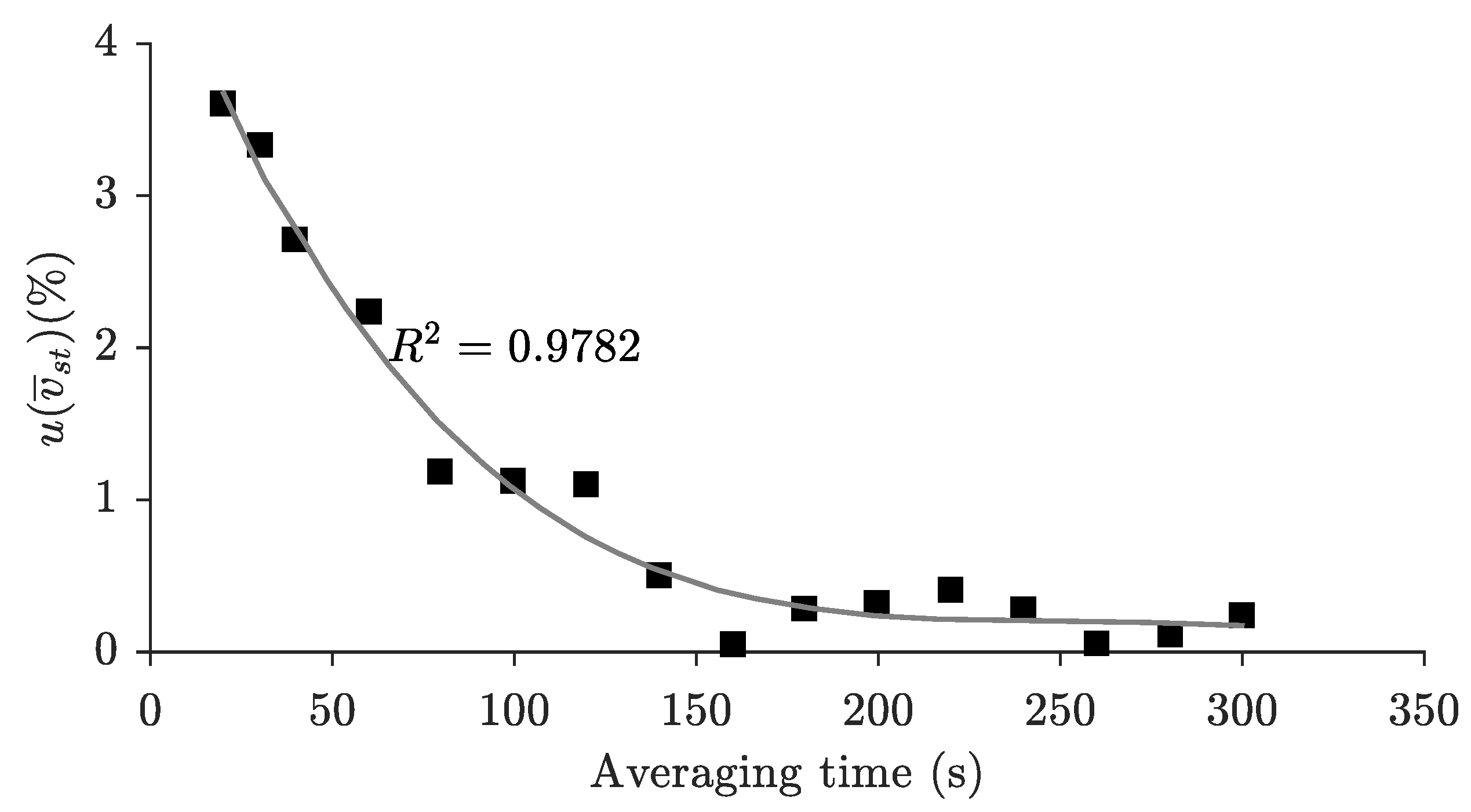
• Sampling time, $u\left({\overline{v}}_{st}\right)$: Velocities at any point in the cross-section are continuously and randomly fluctuating due to turbulence. Sampling the flow over a time interval is required to estimate the mean velocity at a point in order to disregard the turbulence influence. The duration of this measurement is labelled here as sampling time, although other terms are used in the literature such as measuring time [29,30] or exposure time [31]. Sampling time uncertainty is site-dependent, as the flow temporal scales depend on the flow regime, channel geometry and boundary roughness. There is no clear agreement on the appropriate method for selecting the required sampling time [29,31]. One possible solution was applied by [10] by measuring long sampling periods at a fixed position and analyzing the acquired data by applying a cumulative moving average and examining the mean values and dispersion for different time series. The results are shown in Figure 3. The conclusion was that $300$ s sampling time were necessary to stabilise the mean velocity value, which agrees well with previous studies in the literature [32,33]. In this work the sampling time was $60$ s, which according to Figure 3, has an associated standard uncertainty of about 2.5%, consistent with that suggested in Table E.3 of [13].
• Near-transducer, $u\left({\overline{v}}_{tr}\right)$: There is generally a low bias error in the ADCP measurements at the top of the vertical near the transducer. This near-transducer error has different reasons (e.g., ringing, flow disturbance and multi-beam probe configuration) and has been documented in previous studies [34,35]. The full assessment of this source has not been developed in this study and velocity measurements close to the transducer (measurements in the upper $0.4$ m) are simply discarded once the possible effect of the proximity of the transducer has been analyzed.
• Vertical velocity model, $u\left({\overline{v}}_{vd}\right)$: This uncertainty source arises because of the limited number of sampling points in a profile. Table E.4 of [13] defines the uncertainty values that are derived from many samples of irregular vertical velocity curves. Due to the number of measured points in each profile, the measurement method is velocity distribution and the associated uncertainty for this source is $0.5\%$.
• Flow-angle induced error, $u\left({\overline{v}}_{an}\right)$: Flow-angle errors are induced by the deviation of the ADCP orientation from the flow direction. Although Qliner has a compass to automatically correct these errors at the time of the measurements, the ship is not fully stable during the sampling time and a conservative uncertainty of $1\%$ is here considered.
• Operational conditions, $u\left({\overline{v}}_{o}p\right)$: This uncertainty source captures the effects of non-uniformity of suspended scatters in the acoustic beams, tag line deflections, disturbance of the water surface by waves, and operator-induced effects. In order to define this error, a sufficient number of measurements must be made to assess the dispersion of the measured values. Since the accurate estimation of this standard uncertainty has not been performed in this study, the value estimated by [10] ($0.006$ m/s) is used.

2.2.2. Uncertainty Sources Associated with Depth in Verticals, $d_n$

Qliner has a vertical beam (Beam 4) for measuring the depth at the measurement locations. The uncertainty sources associated with depth are listed below according to [10].

• Instrument resolution, $u\left(d_{re}\right)$: Similar to the instrument resolution for velocity measurements, this uncertainty source depends on the last significant digit provided by the Qliner software. Thus, a value of 0.005 m is the standard uncertainty for this source herein, being half of the last significant digit (0.01 m).
• Instrument accuracy, $u\left(d_{ac}\right)$: This uncertainty source depends on the instrument itself and the penetration of the acoustic beam into the bed, which in turn depends on the pulse frequency and consistency of the bed. Therefore, the uncertainty associated with this source is site- and instrument-dependent. End-to-end approaches and specific experiments could be used to assess it accurately like in [10]. However, since the accurate uncertainty estimation has not been accomplished in this study, the standard uncertainty calculated by [10] is assumed, even though it is not the same measurement section or the same instrument. The standard uncertainty for this source is therefore 0.018 m. In addition, this value is consistent with that suggested by table E.2 of [13] for a similar measurement.
• Operational conditions, $u\left(d_{op}\right)$: This uncertainty source involves any consideration that affects the instrument operation: non-uniform concentration of suspended scatters near the bottom, irregular bottom with debris, instabilities in the ship during the measurement, turbulence in water surface by waves and others. The standard uncertainty for this source is 0.0018 m according to [10].

2.2.3. Uncertainty Sources Associated with the Distance between Verticals, $b_n$

The locations of Qliner measurements across the channel were established by setting marks on the tag line of the cable using a measuring tape. In addition, the positions are validated as the depths are measured and the cross-section is known. The uncertainty sources associated with the distance between verticals are listed below.

• Instrument resolution, $u\left(b_{re}\right)$: Similar to the instrument resolution in previous measurements, half of the last significant digit is used as the standard uncertainty. The finest graduation of the measuring tape used is 0.002 m, so the standard uncertainty for this source is 0.001 m.
• Operational conditions, $u\left(b_{op}\right)$: Improper positioning of the verticals during an SxS measurement has negative consequences on the measured velocities and depth, and consequently on the total discharge. The measured cross-sections are known and the vertical positions have been validated by comparing the section measured by the vertical depths and the known section. The standard uncertainty for this source is 0.015 m.

3. Models for Discharge Estimation

This section describes the models for calculating the final discharge from the ADCP velocity measurements. The traditional velocity-area method, specifically the mid-section method, is described, as well as the elemental uncertainties propagation to the final results. Then, the 2D-hydraulic velocity model proposed as an alternative to the velocity-area method is detailed.

3.1. Velocity-Area Method

The velocity-area method consists of a discrete integration of flow velocity over the channel cross-section [10,21]. Each location with data along the vertical profile is characterized by its mean velocity, ${\overline{v}}_n$, and its influence area or area panel, determined by the distance between consecutive locations, $b_n$, and measured depth, $d_n$. Then, total discharge, $Q_t$, is computed by aggregating all panel discharges. Using the notation in Figure 2, the total discharge is defined by:

$$Q_m={\overline{v}}_1{d}_1\left(\frac{b_2-b_1}{2}\right)+\sum _{n=2}^{N-1}\left({\overline{v}}_n{d}_n\left(\frac{b_{n+1}-b_{n-1}}{2}\right)\right)+{\overline{v}}_N{d}_N\left(\frac{b_N-b_{N-1}}{2}\right)$$

(1)

$$Q_t=Q_{LB}+Q_m+Q_{RB}$$

(2)

$$Q_{LB}=0.3535b_1{d}_1{\overline{v}}_1$$

(3)

$$Q_{RB}=0.3535b_{RB}-b_N{d}_N{\overline{v}}_N$$

(4)

where N is the total number of verticals and $b_n$ is the distance of the verticals from the left bank. Therefore, $\left(b_{n+1}-b_{n-1}\right)/2$ is the width associated with the panel at the n-th vertical. Besides, $b_{RB}$ is the distance measured from the left bank to the right bank, i.e., the total width of the cross-section. All variables involved in Equations (1)–(4) are provided by the Qliner software. Above, $Q_{LB}$ and $Q_{RB}$ are the bank flows [36], out of the area covered by direct ADCP measurements, as shown in Figure 2.

The uncertainties described in the previous section are aggregated and propagated to the final discharge results. The final uncertainties associated with the measured variables (mean velocity in the vertical, depth and width) are calculated by aggregating all sources of uncertainty involved in each variable with the following expressions [10]:

$$u({\overline{v}}_n)=\sqrt{u{\left({\overline{v}}_{re}\right)}^2+u{\left({\overline{v}}_{ac}\right)}^2+u{\left({\overline{v}}_{st}\right)}^2+u{\left({\overline{v}}_{vd}\right)}^2+u{\left({\overline{v}}_{an}\right)}^2+u{\left({\overline{v}}_{op}\right)}^2},$$

(5)

$$u(d_n)=\sqrt{u{\left(d_{re}\right)}^2+u{\left(d_{ac}\right)}^2+u{\left(d_{op}\right)}^2},$$

(6)

$$u(b_n)=\sqrt{u{\left(b_{re}\right)}^2+u{\left(b_{op}\right)}^2},$$

(7)

and the expanded uncertainty for the discharge is then given by

$$u_c(Q_t)=\sqrt{\sum _{n=1}^{N}u{\left({\overline{v}}_n\right)}^2{\left(\frac{\mathsf{\partial }{Q}_t}{{\overline{v}}_n}\right)}^2+\sum _{n=1}^{N}u{\left(d_n\right)}^2{\left(\frac{\mathsf{\partial }{Q}_t}{d_n}\right)}^2+\sum _{n=1}^{N}u{\left(b_n\right)}^2{\left(\frac{\mathsf{\partial }{Q}_t}{b_n}\right)}^2},$$

(8)

$$U\left(Q_t\right)=k{u}_c\left(Q_t\right).$$

(9)

Note that Equation (8) is a first-order Taylor approximation used to propagate the uncertainty of each variable to the final discharge results. In addition of these terms, the contribution of correlated uncertainties should be added because the total discharge is the sum of the discharge of consecutive panels where velocities, depths and widths have been measured with the same instrument. However, even though the three measured variables are affected by correlated uncertainties (they are not independent variables), these terms are difficult to estimate [10], and therefore they are assumed to be zero in the present analysis. Finally, a coverage coefficient k of 2 corresponding to a confidence level of approximately 95% is considered for calculating the final uncertainty [18].

3.2. Proposed Method: The 2D-Hydraulic Velocity Model (2D-HVM)

An alternative to the velocity-area method is the employment of a numerical model to reproduce the velocity distribution within the whole cross section. Recently, [24] improved and validated a 2D streamwise velocity model based on the RANS equations using different cross-section shapes (circular, rectangular, trapezoidal and compound section) and roughness conditions with quite good agreement with experimental values, and also including the effects of free surface boundary layer. The original numerical model is only suitable for straight channels since for symmetric cross-sections it leads to symmetric velocity distributions. A modification of the numerical model to aggregate the effect of the asymmetry of the flow near bends is here proposed. The partial differential equation to be solved in [24] is given by

$$\frac{\mathsf{\partial }}{\mathsf{\partial }y}\left((\nu +{\nu }_t)\frac{\mathsf{\partial }u}{\mathsf{\partial }y}\right)+\frac{\mathsf{\partial }}{\mathsf{\partial }z}\left((\nu +{\nu }_t)\frac{\mathsf{\partial }u}{\mathsf{\partial }z}\right)=-g{S}_f,$$

(10)

being $u\equiv$ the streamwise velocity in $x-$ direction, $\nu \equiv$ the kinematic viscosity of the fluid, ${\nu }_t\equiv$ the eddy viscosity, $S_f\equiv$ the friction slope and y and z the transverse and vertical direction respectively. The reader is referred to the original work for more details. The gravitational action given by the term $-g{S}_f$ in Equation (10) can be modified considering it linearly dependent on the cross-stream position (y) instead of constant over the whole section. Equation (10) therefore becomes as follows:

$$\frac{\mathsf{\partial }}{\mathsf{\partial }y}\left((\nu +{\nu }_t)\frac{\mathsf{\partial }u}{\mathsf{\partial }y}\right)+\frac{\mathsf{\partial }}{\mathsf{\partial }z}\left((\nu +{\nu }_t)\frac{\mathsf{\partial }u}{\mathsf{\partial }z}\right)=-gmax\left[S_f+m_{S_f}y,S_{f_{min}}\right],$$

(11)

where $m_{S_f}\equiv$ is the variation of the friction slope in the cross-stream direction with the centre of the cross-section at $y=0$ and $S_{f_{min}}$ is the minimum friction slope assumed (${10}^{-6}$). The minimum value is always positive, due to the fact that the flow cannot reverse, therefore the friction slope cannot have an opposite sign to the flow direction. Once the numerical model is solved, it allows the numerical integration of the velocity distribution to obtain the total flow discharge.

4. State Estimation

State Estimation (SE) techniques allow the hydraulic model to be fitted to adequately reproduce the measurements, and to perform the uncertainty analysis propagating the elemental uncertainty sources to the final results.

For a given set of variables related with a system of governing equations, the state variables (unknown variables) are the minimum number of variables that set the state of the full system. A SE algorithm enables the most likely value of the state variables to be computed by combining the information provided by a set of imperfect measurements and a system of governing equations [26]. In general terms, the SE problem is based on the following model:

$$\mathbf{z}=\mathbf{g}(\mathbf{x})+\mathbf{e}.$$

(12)

where $\mathbf{z}\in {\mathbb{R}}^m\equiv$ is the measurement vector (measured velocities and water depths); $\mathbf{x}\in {\mathbb{R}}^n\equiv$ is the state variables vector (unknown parameters of the numerical model to be calibrated); g: ${\mathbb{R}}^n\to {\mathbb{R}}^m\equiv$ is the relationship between measurements and state variables (given by the governing equations); and $\mathbf{e}\equiv$ is the measurement error vector (typically assumed to be Gaussian with zero mean, i.e., unbiased, with the variance-covariance matrix ${\mathbf{R}}_{\mathbf{z}}$) [26,37].

SE methods use statistical criteria to estimate the actual value of those unknown variables. One option is to solve the weighted least squares (WLS) problem given by

$$\underset{\mathbf{x}}{min}F(\mathbf{x})={\mathbf{e}}^T{{\mathbf{R}}_{\mathbf{z}}}^{-1}\mathbf{e}={[\mathbf{z}-\mathbf{g}\mathbf{x}]}^T{{\mathbf{R}}_{\mathbf{z}}}^{-1}[\mathbf{z}-\mathbf{g}(\mathbf{x})].$$

(13)

Since the governing equations here involve a nonlinear relationship between the measurements and the state variables, it can only be computed in an iterative way using the well-known Gauss-Newton method between successive iterations [38,39], i.e.:

$$\begin{array}{c}\Delta {\mathbf{x}}_{i+1}={\left[{\mathbf{J}}_i^T{{\mathbf{R}}_{\mathbf{z}}}^{-1}{\mathbf{J}}_i\right]}^{-1}\left[{\mathbf{J}}_i^T{{\mathbf{R}}_{\mathbf{z}}}^{-1}\right][\mathbf{z}-\mathbf{g}\left({\mathbf{x}}_i\right)]\\ {\mathbf{x}}_{i+1}={\mathbf{x}}_i+\Delta {\mathbf{x}}_{i+1}\end{array}$$

(14)

where ${\mathbf{J}}_i\in {\mathbb{R}}^{m\times n}\equiv$ is the Jacobian matrix which represents the sensitivity of the measurements with respect to the state variables at iteration i. In addition, the SE uncertainty can also be estimated by computing the variance-covariance matrix for the state variables (${\mathbf{R}}_{\mathbf{x}}$) according to the following formulation [26]:

$${\mathbf{R}}_{\mathbf{x}}={\left[{\mathbf{J}}^T{{\mathbf{R}}_{\mathbf{z}}}^{-1}\mathbf{J}\right]}^{-1}$$

(15)

Application of SE to the Hydraulic Model

In Equation (12), the state variables x are the inputs of the hydraulic model, that in the considered numerical model are: friction slope ($S_f$), boundary roughness ($k_s$), water level (H) and the transverse variation of the friction slope ($m_{S_f}$). The parameter $m_{S_f}$ is considered as a state variable only in the case of an asymmetric velocity distribution, i.e., for GG7. Note that state variables include traditionally referred as parameters (e.g., boundary roughness), beside variables (e.g., friction slope or water level). The major difference comes from the persistence of their values over time (longer or permanent for parameters). In the SE context, both can be considered state variables. The measurements vector, z, is constituted by the column vector, d, containing the depth of each vertical ($d_n$) and the column vectors containing all measured velocities $V_X$ and $V_{X3}$ obtained by the ADCP. The non-linear relationship between measurements and state variables $\mathbf{g}\left(\mathbf{x}\right)$ is the hydraulic model described in the previous section. The Jacobian matrix J relating the measurements with the state variables is constructed as follows:

$$\mathbf{J}=\left[\begin{array}{cccc}\frac{\mathsf{\partial }\mathbf{d}}{\mathsf{\partial }{s}_f}& \frac{\mathsf{\partial }\mathbf{d}}{\mathsf{\partial }{k}_s}& \frac{\mathsf{\partial }\mathbf{d}}{\mathsf{\partial }H}& \frac{\mathsf{\partial }\mathbf{d}}{\mathsf{\partial }{m}_{S_f}}\\ \frac{\mathsf{\partial }{V}_X}{\mathsf{\partial }{s}_f}& \frac{\mathsf{\partial }{V}_X}{\mathsf{\partial }{k}_s}& \frac{\mathsf{\partial }{V}_X}{\mathsf{\partial }H}& \frac{\mathsf{\partial }{V}_X}{\mathsf{\partial }{m}_{S_f}}\\ \frac{\mathsf{\partial }{V}_{X_3}}{\mathsf{\partial }{S}_f}& \frac{\mathsf{\partial }{V}_{X_3}}{\mathsf{\partial }{k}_s}& \frac{\mathsf{\partial }{V}_{X_3}}{\mathsf{\partial }H}& \frac{\mathsf{\partial }{V}_{X_3}}{\mathsf{\partial }{m}_{S_f}}\end{array}\right].$$

(16)

The variance-covariance matrix of the measurements, ${\mathbf{R}}_{\mathbf{z}}$, consists of the uncertainties associated with the measurements. The uncertainty of the depth of the verticals, $u\left(d_n\right)$, is directly calculated with the Equation (6), whereas the uncertainties of the measured velocities, $u\left(V_X\right)$ and $u\left(V_{X3}\right)$, are calculated with the Equation (5). Besides, the uncertainty of the distance between verticals, $u\left(b_n\right)$, must be also included even when this variable is not inside the measurements vector. In order to consider it, the potential changes of the velocities when changing the position of the verticals are assessed. This requires using the velocity distribution of the hydraulic model and the uncertainty associated with the distance between verticals, $u\left(b_n\right)$, calculated with Equation (7). Therefore, the following terms must be aggregated to the uncertainties of the measured velocities $u\left(V_X\right)$ and $u\left(V_{X3}\right)$:

$$u\left(V_{X_b}\right)=\left[u\left(b_n\right)\left(\frac{\mathsf{\partial }{V}_X}{\mathsf{\partial }{b}_n}\right)\right],\mathrm{and}u\left(V_{X{3}_b}\right)=\left[u\left(b_n\right)\left(\frac{\mathsf{\partial }{V}_{X3}}{\mathsf{\partial }{b}_n}\right)\right].$$

(17)

Finally, once the uncertainty of the distance between verticals is accounted for into the uncertainty of the measured velocities, the variance-covariance matrix of the measurements ${\mathbf{R}}_{\mathbf{z}}$ is constituted by the vector $[u{(d_n)}^2;u{(V_X)}^2;u{(V_{X3})}^2]$ on its diagonal and by the covariances between the velocities measured on the same vertical:

$${\mathbf{R}}_{\mathbf{z}}=\left[\begin{array}{ccc}u{(d_n)}^2& u(d_n)u(V_X)& u(d_n)u(V_{X3})\\ u(V_X)u(d_n)& u{(V_X)}^2& u(V_X)u(V_{X3})\\ u(V_{X3})u(d_n)& u(V_{X3})u(V_X)& u{(V_{X3})}^2\end{array}\right].$$

(18)

Equation (14) is applied iteratively yielding a new value for the state variables at every iteration. The Gauss-Newton method is an approximate iterative method based on problem linearization. It is applied until the state variables reach their optimal value that minimizes the differences between measurement and model results. Once the optimal value of the state variables is reached, the variance-covariance matrix of the state variables can be calculated by applying the Equation (15). This matrix provides the uncertainty of the state variables and can be expressed as:

$${\mathbf{R}}_{\mathbf{x}}=\left[\begin{array}{cccc}u{\left(S_f\right)}^2& u\left(S_f\right)u\left(k_s\right)& u\left(S_f\right)u\left(H\right)& u\left(S_f\right)u(m_{S_f})\\ u(k_s)u(S_f)& u{(k_s)}^2& u(k_s)u(H)& u(k_s)u(m_{S_f})\\ u(H)u(S_f)& u(H)u(k_s)& u{(H)}^2& u(H)u(m_{S_f})\\ u(m_{S_f})u\left(S_f\right)& u(m_{S_f})u(k_s)& u(m_{S_f})u(H)& u{(m_{S_f})}^2\end{array}\right].$$

(19)

Then, since the hydraulic model provides the velocity distribution of the whole cross-section, the total discharge is a derived variable and its uncertainty can be calculated with the following expression:

$$u_c{\left(Q_t\right)}^2=\left[\begin{array}{cccc}\frac{\mathsf{\partial }{Q}_t}{\mathsf{\partial }{S}_f}& \frac{\mathsf{\partial }{Q}_t}{\mathsf{\partial }{k}_s}& \frac{\mathsf{\partial }{Q}_t}{\mathsf{\partial }H}& \frac{\mathsf{\partial }{Q}_t}{\mathsf{\partial }{m}_{S_f}}\end{array}\right]{\mathbf{R}}_x{\left[\begin{array}{cccc}\frac{\mathsf{\partial }{Q}_t}{\mathsf{\partial }{S}_f}& \frac{\mathsf{\partial }{Q}_t}{\mathsf{\partial }{k}_s}& \frac{\mathsf{\partial }{Q}_t}{\mathsf{\partial }H}& \frac{\mathsf{\partial }{Q}_t}{\mathsf{\partial }{m}_{S_f}}\end{array}\right]}^T$$

(20)

$$U\left(Q_t\right)=k{u}_c\left(Q_t\right)$$

(21)

5. Results

This section presents the results of the application of the velocity-area method and the 2D-HVM new approach for the discharge estimation and its associated uncertainty. The improvement in final uncertainty resulting from propagating the uncertainty of direct measurements is quantified, without assessing the inherent uncertainties of the models, which will be better in the case of the 2D-HVM approach, since it is a physically based and tested model. First, results for measurements in section GG11, which has a symmetrical velocity distribution, are presented. Finally, results for measurements in section GG7 are presented, which is characterised by an asymmetric velocity distribution due to its location downstream of a slight channel bend.

5.1. Measurements in GG11

Three sets of ADCP measurements at different dates were taken in section GG11, each set consisting of two independent SxS measurements (a and b). Each measurement consists of 12 measured verticals spaced horizontally 1 m to cover the total width of the channel. The detailed results from the application of the velocity-area method and the adjusted hydraulic model are presented in

Table 2. Results for measurements of section GG11. Coverage coefficient—$k=2$.

Set	Id	Water Level	Velocity-Area Method			2D-HVM Method
			${\mathit{Q}}_{\mathit{t}}$	$\mathit{U}({\mathit{Q}}_{\mathit{t}})$	$\mathit{U}({\mathit{Q}}_{\mathit{t}})$	${\mathit{Q}}_{\mathit{t}}$	$\mathit{U}({\mathit{Q}}_{\mathit{t}})$	$\mathit{U}({\mathit{Q}}_{\mathit{t}})$
		(m)	(m3/s)	(m3/s)	(%)	(m3/s)	(m3/s)	(%)
1	a	3.425	38.252	1.413	3.693	38.227	0.260	0.679
1	b	3.421	37.802	1.403	3.712	38.071	0.260	0.682
2	a	3.401	34.769	1.293	3.717	34.969	0.239	0.684
2	b	3.401	34.808	1.289	3.704	34.917	0.239	0.684
3	a	3.521	37.531	1.391	3.707	37.330	0.251	0.672
3	b	3.511	37.621	1.386	3.685	37.759	0.250	0.662

.

Overall, the computed discharges using both methods are consistent and there are no significant differences between them, being the values within the confidence intervals defined by their final uncertainties. The main advantages of using the 2D-HVM method are that the velocity distribution is estimated over the whole cross-section thanks to the 2D-RANS streamwise modelization, accounting in the computation for the real governing equations that describe the phenomena, and the physical relationships among measurements. Thus, the uncertainty values for the computed discharge are much lower than those using the velocity-area method, yielding to a higher confidence of estimated discharge. Note that, even though only uncertainties associated with the direct measured variables are considered, the uncertainties associated to the final discharge are notable in the case of the velocity-area method, greater than $3.6\%$ in all cases. Those values are reduced below $0.7\%$ when using the adjusted hydraulic model. In addition to this improvement by propagating the uncertainties of the direct measurements, the uncertainty inherent of the discharge model, although not assessed, will also be lower since it uses a 2D-RANS model, which incorporates the most important physical phenomena involved and has been extensively validated under many different real conditions.

Besides, using proposed method allows obtaining the most probable value of the state variables and their associated uncertainties, as shown in

Table 3. Optimal state variables and their associated uncertainties in section GG11 from SE. Coverage coefficient—$k=1$.

Set	Id	${\mathit{S}}_{\mathit{f}}$	$\mathit{u}({\mathit{S}}_{\mathit{f}})$	${\mathit{k}}_{\mathit{s}}$	$\mathit{u}({\mathit{k}}_{\mathit{s}})$	H	$\mathit{u}(\mathit{H})$
		(−)	(−)	(m)	(m)	(m)	(m)
		($\times {\mathbf{10}}^{-\mathbf{4}}$)	($\times {\mathbf{10}}^{-\mathbf{4}}$)	($\times {\mathbf{10}}^{-\mathbf{4}}$)	($\times {\mathbf{10}}^{-\mathbf{4}}$)
1	a	1.774	0.097	1.482	0.884	3.426	0.005
1	b	1.864	0.111	2.521	0.884	3.421	0.005
2	a	1.758	0.073	4.296	0.994	3.400	0.005
2	b	1.790	0.087	4.814	1.302	3.399	0.005
3	a	1.838	0.078	6.687	1.792	3.519	0.005
3	b	1.788	0.081	4.628	1.249	3.512	0.005

. This additional information could help to adequately manage hydraulic structures. For instance, in the analyzed case, the estimated boundary roughness, $k_s$, increases with time, which is congruent with the growth of benthic algae experienced in this irrigation channel.

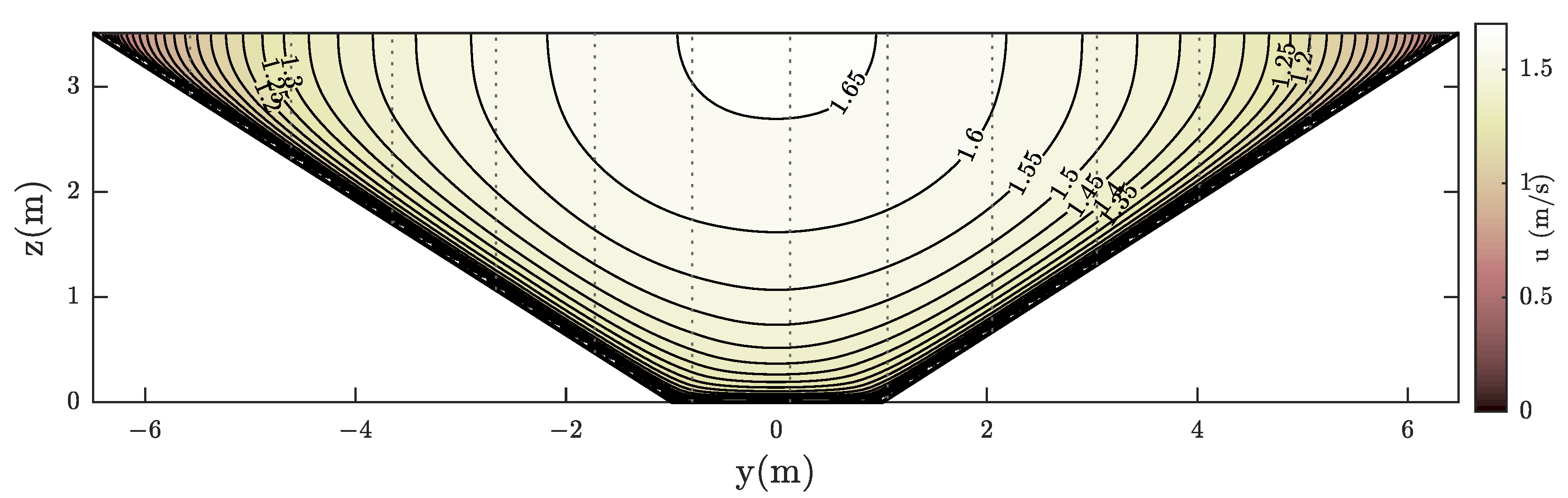
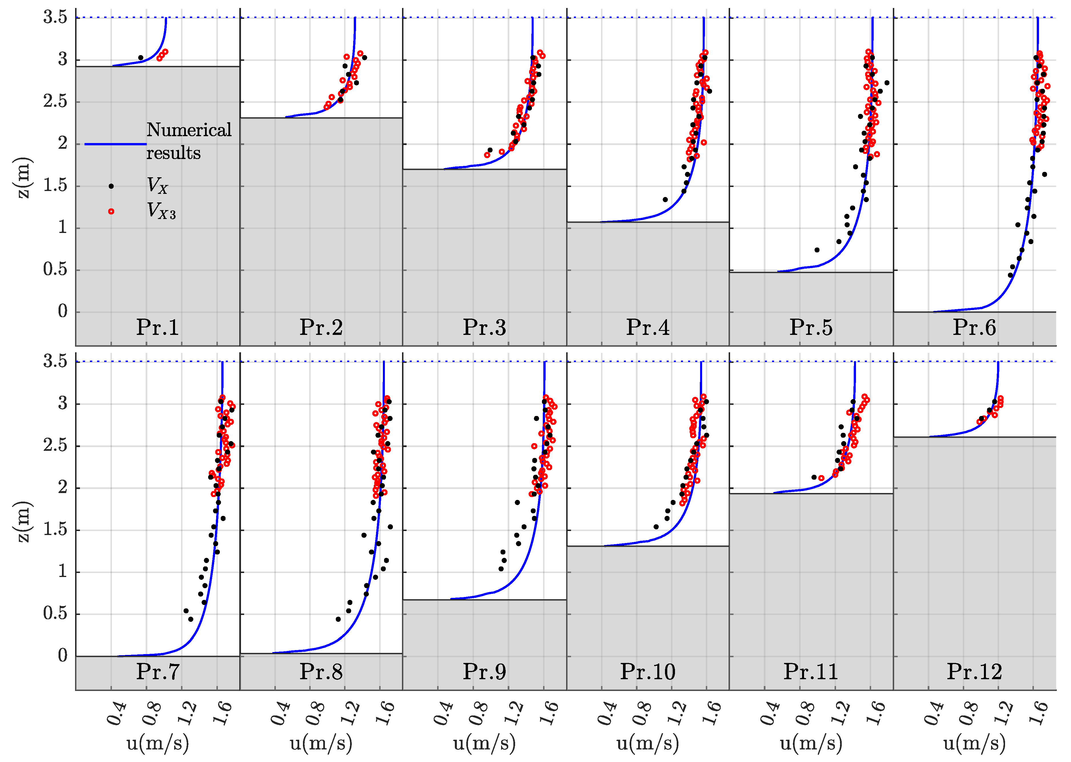
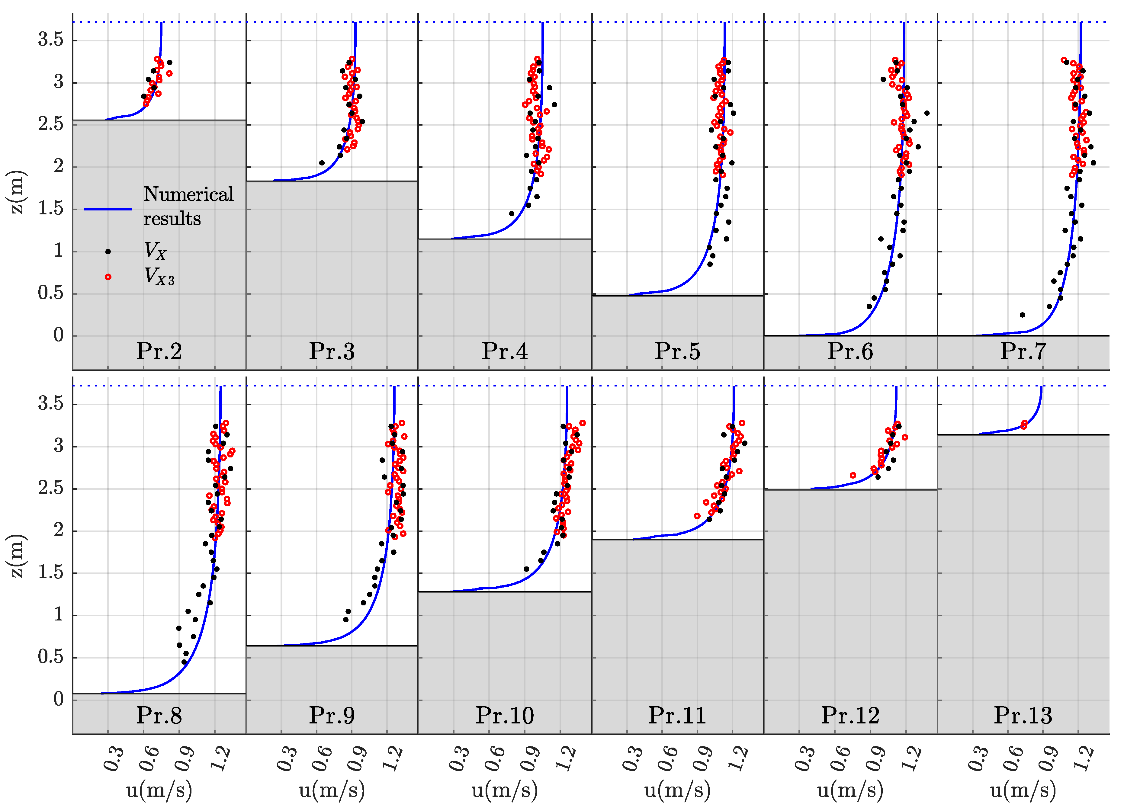
Figure 4 represents the velocity distribution of the hydraulic model for measurement 3b. The position of all measured verticals is shown with grey dashed lines. Figure 5 represents all velocity profiles of the measured verticals where the model results and the measured velocities ($V_X$ and $V_{X3}$) are shown. The velocity profiles illustrate that the coherence between the model results and the measured velocities is quite good. Hence, the hydraulic model is able to reliably reproduce the measurements.

Coherence between different measurements of the same set, a and b, is also observed in all cases and for both methods. Small differences between both are probably caused by small flow unsteadiness or regime change during the measurement. However, they are all consistent and there is a wide overlap of their confidence intervals.

5.2. Measurements in GG7

Similarly to section GG11, three sets of ADCP measurements at different times were made in section GG7. Each measurement consists of 12 or 13 measured verticals spaced horizontally 1 m to cover the total width of the channel. The detailed results from the application of the velocity-area method and the adjusted hydraulic model are presented in

Table 4. Results for measurements of section GG7. Coverage coefficient—$k=2$.

Set	Id	Water Level	Velocity-Area Method			2D-HVM Method
			${\mathit{Q}}_{\mathit{t}}$	$\mathit{U}({\mathit{Q}}_{\mathit{t}})$	$\mathit{U}({\mathit{Q}}_{\mathit{t}})$	${\mathit{Q}}_{\mathit{t}}$	$\mathit{U}({\mathit{Q}}_{\mathit{t}})$	$\mathit{U}({\mathit{Q}}_{\mathit{t}})$
		(m)	(m3/s)	(m3/s)	(%)	(m3/s)	(m3/s)	(%)
1	a	3.636	28.303	1.030	3.638	28.453	0.202	0.711
1	b	3.641	28.514	1.041	3.651	28.798	0.201	0.697
2	a	3.716	29.476	1.074	3.644	29.608	0.191	0.645
2	b	3.721	29.683	1.080	3.635	29.922	0.195	0.651
3	a	3.656	25.477	0.926	3.636	25.378	0.169	0.668
3	b	3.643	25.620	0.937	3.656	25.732	0.166	0.647

.

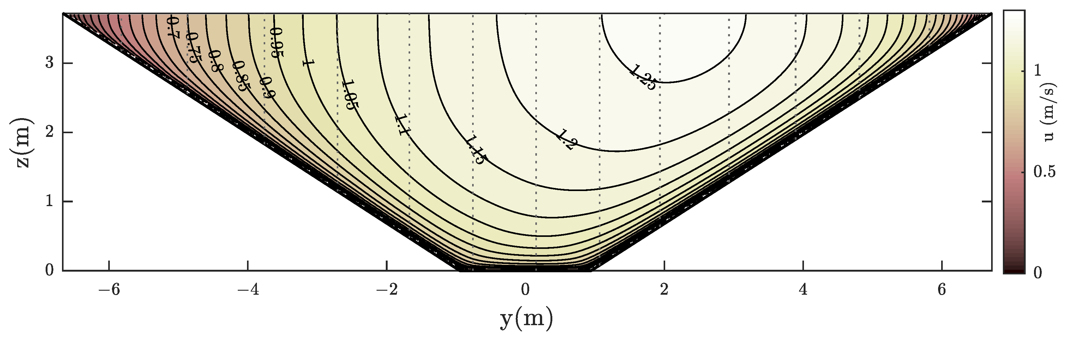
The results in section GG7 support the conclusions induced by section GG11, validating the hydraulic model as a good alternative to the velocity-area method. Again, the discharges of both methods are coherent and there are no significant differences between them. There is a notable region of overlap between the confidence intervals derived from the application of both methods. The discharge confidence interval of the hydraulic model is entirely within the one of the velocity-area method. Another example of the good behaviour of the hydraulic model is presented in Figure 6 and Figure 7. In this case, the measurement corresponds to 2b case. Figure 6 represents the velocity distribution of the hydraulic model which is asymmetric (downstream of a slight bend). Unlike the previous case, the variation of the friction slope has been considered as a state variable. Its value is estimated with the SE process together with the rest of the state variables. Figure 7 represents the velocity profiles of the measured verticals where the model results and the measured velocities ($V_X$ and $V_{X3}$) are presented. There is again very good agreement between the results of the hydraulic model and the measurements, and the hydraulic model replicates the measurements closely even with asymmetric velocity distribution.

Coherence between successive measurements remains in section GG7, which validates the measurements used in this study. Regarding the uncertainty associated to the final discharge, its value is again considerably smaller when applying the hydraulic model (≲$0.7\%$) compared to the velocity-area method (≳$3.6\%$). The optimal state variables for all measurements in section GG7, as well as their associated uncertainties, are shown in

Table 5. Optimal state variables and their associated uncertainties in section GG7 from SE. Coverage coefficient—$k=1$.

Set	Id	${\mathit{S}}_{\mathit{f}}$	$\mathit{u}({\mathit{S}}_{\mathit{f}})$	${\mathit{k}}_{\mathit{s}}$	$\mathit{u}({\mathit{k}}_{\mathit{s}})$	H	$\mathit{u}(\mathit{H})$	${\mathit{m}}_{{\mathit{S}}_{\mathit{f}}}$	$\mathit{u}({\mathit{m}}_{{\mathit{S}}_{\mathit{f}}})$
		(−)	(−)	(m)	(m)	(m)	(m)	(−)	(−)
		($\times {\mathbf{10}}^{-\mathbf{4}}$)	($\times {\mathbf{10}}^{-\mathbf{4}}$)	($\times {\mathbf{10}}^{-\mathbf{4}}$)	$\times {\mathbf{10}}^{-\mathbf{4}}$			($\times {\mathbf{10}}^{-\mathbf{5}}$)	($\times {\mathbf{10}}^{-\mathbf{5}}$)
1	a	1.029	0.059	7.524	2.244	3.635	0.005	1.990	0.113
1	b	0.098	0.048	5.060	1.227	3.638	0.005	1.781	0.085
2	a	0.098	0.055	6.440	1.738	3.715	0.005	2.109	0.106
2	b	1.073	0.048	9.867	2.642	3.720	0.005	1.975	0.090
3	a	0.088	0.049	12.04	3.562	3.655	0.005	1.532	0.082
3	b	0.080	0.044	5.839	1.540	3.643	0.005	1.619	0.086

.

6. Conclusions

A new alternative to the conventional velocity-area method for calculating the total discharge and its associated uncertainty from SxS measurements with ADCP in open channels is presented. The velocity-area method is commonly used to calculate the discharge from ADCP measurements. This method, which has both mid-section and mean-section options, consists of a discrete integration of the partial discharge of the cross-section panels which are defined by the measured verticals. Since this is a discrete integration, the two dimensions of the cross-section are integrated independently, meaning that the mean velocity in one profile is independent of the adjacent profile data, even where there is a hydraulic relationship between their velocities by proximity. Instead of considering vertical and horizontal integration independently, the proposed 2D-HVM method integrates them together and takes advantage of the relationships between them. For this purpose, the new methodology uses the 2D-RANS model, an affordable and proven numerical model to compute the longitudinal velocity distribution in an open-channel. The 2D-RANS model is fitted using state estimation techniques to accurately reproduce the measurement field and the behaviour of the free-surface stream. The good performance of the 2D-RANS model and its fitting process have been validated with measurements on two different trapezoidal cross-section of a real channel. Moreover, the good performance remains even with asymmetric velocity distributions caused by a slight upstream bend in one of the measured sections. Besides reproducing the measurement field faithfully in all cases, the hydraulic model provides the velocity distribution over the entire cross-section. Then, measurement information is extrapolated to positions where there are no measurements without making non-hydraulic assumptions, i.e. the connections between measurements have a solid and consistent hydraulic basis.

The new 2D-HVM method produces discharge estimations consistent with velocity-area method, but with a significant uncertainty reduction, considering only measurement uncertainties propagation. Furthermore, the measurement information is further enhanced, since it is considered together rather than isolated by verticals, and allows the final uncertainty of the discharge to be reduced. In the uncertainty analysis, only the uncertainties associated with the directly measured variables have been considered and propagated to the final results. Thus, an objective comparison is achieved without assessing the uncertainty associated with the computing models as well as other uncertainties independent of the direct measurements. Because uncertainty associated to the model is also better for 2D-RANS model than for the purely empirical assumptions about the 2D velocity field map used for the velocity-area methods, the total confidence of the 2D-HVM is superior to the velocity-area method.

Another advantage of the proposed method is the possibility to assess the uncertainty effect of considering more or less number of measurements, e.g., by changing the distance between verticals. Typically, a significant portion of the final uncertainty when applying the velocity-area method depends on the number of verticals, whose standard uncertainty is based on an empirical function which does not consider the spatial distribution of verticals or the flow distribution. This uncertainty source, which has not been accounted (inherent uncertainty) in this study to compare both methods, can be assessed objectively with the proposed method. Furthermore, the hydraulic model clearly allows outliers to be detected. Then, those measurements inconsistent with their position and environment are detected, and thus the measurements can be validated.

References

- Rantz, S.E. Measurement and Computation of Streamflow. Vol. 1, Measurement of Stage and Discharge, 1st ed.; Water-Supply Paper 2175; US Geological Survey: Washington, DC, USA, 1982.
- Morlock, S.E. Evaluation of Acoustic Doppler Current Profiler Measurements of River Discharge; Water-Resources Investigations Report 95-4218; U.S. Geological Survey: Indianapolis, IN, USA, 1996.
- Oberg, K.A.; Mueller, D. Validation of stream flow measurements made with acoustic Doppler current profilers. J. Hydraul. Eng. 2007, 12, 1421–1432. [Google Scholar] [CrossRef] [Green Version]
- Simpson, M.R. Discharge Measurements Using a Broad-Band Acoustic Doppler Current Profiler; Open-File Report 01-1.; U.S. Geological Survey: Sacramento, CA, USA, 2001.
- Mueller, D.S.; Wagner, C.R.; Rehmel, M.S.; Oberg, K.A.; Rainville, F. Measuring Discharge with Acoustic Doppler Current Profilers from a Moving Boat: U.S. Geological Survey Techniques and Methods 3-A22; U.S. Geological Survey: Reston, VA, USA, 2013.
- Gordon, R.L. Acoustic Measurement of River Discharge. J. hydraul. Eng. 1989, 115, 925–936. [Google Scholar] [CrossRef]
- Oberg, K.A.; Mueller, C.D. Recent Applications of Acoustic Doppler Current Profilers. In Proceedings of the Symposium on Fundamentals and Advancements in Hydraulic Measurements and Experimentation, Buffalo, NY, USA, 1 August 1994; ASCE: New York, NY, USA, 1994; pp. 341–350. [Google Scholar]
- Pelletier, P.M. Uncertainties in the single determination of river discharge: A literature review. Can. J. Civ. Eng. 1988, 15, 834–850. [Google Scholar] [CrossRef]
- Sauer, V.B. Determination of Error in Individual Discharge Measurements; Open-File Report 92-144; US Geological Survey: Norcross, GA, USA, 1992; p. 21.
- Lee, K.; Ho, H.; Muste, M.; Wu, C. Uncertainty in open channel discharge measurements acquired with StreamPro ADCP. J. Hydrol. 2014, 509, 101–114. [Google Scholar] [CrossRef]
- Muste, M.; González-Castro, J.A.; Starzmann, E. Methodology for estimating ADCP measurement uncertainty in open-channel flows. In Proceedings of the World Water & Environmental Resources Congress, Salt Lake City, UT, USA, 27 June–1 July 2004. [Google Scholar]
- ISO/TS 25377. Hydrometric Uncertainty Guidance (HUG); International Organization for Standardization: Geneva, Switzerland, 2007; p. 51. [Google Scholar]
- ISO 748. Hydrometry—Measurement of Liquid Flow in Open Channels Using Current-Meters or Floats; International Organization for Standardization: Geneva, Switzerland, 2007; p. 46. [Google Scholar]
- AIAA. Assessment of Wind Tunnel Data Uncertainty; AIAA S-071-1995; American Institute of Aeronautics and Astronautics (AIAA): Washington, DC, USA, 1995. [Google Scholar]
- ASME. Test Uncertainty: Instruments and Apparatus; PTC 19.1-1998; American Society of Mechanical Engineers (ASME): New York, NY, USA, 1998. [Google Scholar]
- ISO. Guide to the Expression of Uncertainty in Measurement, 1st ed.; International Organization for Standardization: Geneva, Switzerland, 1993. [Google Scholar]
- Herschy, R.W. The uncertainty in a current meter measurement. Flow Meas. Instrum. 2002, 13, 281–284. [Google Scholar] [CrossRef]
- GUM. Evaluation of Measurement Data—Guide to the Expression of Uncertainty in Measurement; JGGM Member Organizations (BIPM, IEC, IFCC, ILAC, ISO, IUPAC, IUPAP and OIML): Geneva, Switzerland, 2008; p. 120. [Google Scholar]
- Muste, M.; Lee, K.; Bertrand-Krajewski, J. Standardized uncertainty analysis for hydrometry: A review of relevant approaches and implementation examples. Hydrol. Sci. J. 2012, 57, 643–669. [Google Scholar] [CrossRef] [Green Version]
- Muste, M. Guidelines for the Assessment of Uncertainty of Hydrometric Measurements. Commission for Hydrology Project: Assessment of the Performance of Flow Measurement Instruments and Techniques; World Meteorological Organization–Weather, Climate and Water: Iowa City, IA, USA, 2009. [Google Scholar]
- Le Coz, J.; Camenen, B.; Peyrard, X.; Dramais, G. Uncertainty in open-channel discharges measured with the velocity-area method. Flow Meas. Instrum. 2012, 26, 18–29. [Google Scholar] [CrossRef] [Green Version]
- Kean, J.W.; Kunhle, R.A.; Smith, J.D.; Alonso, C.V.; Langendoen, E.J. Test of a method to calculate near-bank velocity and boundary shear stress. J. Hydraul. Eng. 2009, 135, 588–601. [Google Scholar] [CrossRef]
- Cassan, L.; Roux, H.; Dartus, D. Velocity distribution in open channel flow with spatially distributed roughness. Environ. Fluid Mech. 2020, 20, 321–338. [Google Scholar] [CrossRef]
- Figuérez, J.A.; Galán, A.; González, J. An enhanced treatment of boundary conditions for 2D RANS streamwise velocity models in open channel flow. Water 2021, 13, 1001. [Google Scholar] [CrossRef]
- Powell, R.; Irving, M.; Sterling, M. A comparison of three real-time state estimation methods for on-line mointoring of water distribution systems. In Computer Applications in Water Supply. Volume 1: Systems Analysis and Simulation; Coulbeck, B., Orr, C., Eds.; Research Studies Press Ltd.: Taunton, UK, 1988; pp. 333–348. [Google Scholar]
- Diaz, S.; González, J.; Mínguez, R. Uncertainty evaluation for constrained state estimation in water distribution systems. J. Water Resour. Plan. Manag. 2016, 142, 12. [Google Scholar] [CrossRef]
- Kapelan, Z.; Savic, D.; Walters, G. Multiobjective sampling design for water distribution model calibration. J. Water Resour. Plan. Manag. 2003, 129, 466–479. [Google Scholar] [CrossRef]
- Diaz, S.; González, J.; Mínguez, R. Calibration via multi-period state estimation in water distribution systems. Water Resour. Manag. 2017, 31, 4801–4819. [Google Scholar] [CrossRef]
- ISO 1088. Hydrometry-Velocity-Area Methods Using Current-Meters-Collection and Processing of Data for Determination of Uncertainties in Flow Measurement; International Organization for Standardization: Geneva, Switzerland, 2007. [Google Scholar]
- Herscy, R.W. Streamflow Measurement; Routledge. Taylor & Francis Group: London, UK, 2009. [Google Scholar]
- Garcia, C.M.; Tarrab, L.; Oberg, K.; Szupianny, R.; Cantero, M.I. Variance of discharge estimates sampled using ADCP’s from moving platforms. J. Hydraul. Eng. 2012, 138, 684–694. [Google Scholar] [CrossRef]
- Stone, M.C.; Hotchkiss, R.H. Evaluating velocity measurement techniques in shallow streams. J. Hydraul. Res. 2007, 45, 752–762. [Google Scholar] [CrossRef]
- Szupiany, R.N.; Amsler, M.L.; Best, J.L.; Parsons, D.R. Comparison of fixed- and moving-vessel flow measurements with an aDP in a large river. J. Hydraul. Eng. 2007, 133, 1299–1309. [Google Scholar] [CrossRef]
- Mueller, D.S.; Abad, J.D.; García, C.M.; Gartner, J.W.; García, M.H.; Oberg, K.A. Errors in acoustic Doppler profiler velocity measurements caused by flow disturbance. J. Hydraul. Eng. 2007, 133, 1411–1420. [Google Scholar] [CrossRef] [Green Version]
- Muste, M.; Kim, D.; Gonzalez-Castro, J.A. Near-transducer errors in ADCP measurements: Experimental findings. J. Hydraul. Eng. 2010, 136, 275–289. [Google Scholar] [CrossRef]
- Fulford, J.M.; Sauer, V.B. Comparison of velocity interpolation methods for computing open-channel discharge. In Selected Papers in the Hydrologic Sciences: US Geological Survey Water-Supply Paper; Volume 2290; Subitsky, S.Y., Ed.; US Geological Survey: Reston, VA, USA, 2007; pp. 139–144. [Google Scholar]
- Brandalik, R.; Wellssow, W. Power system state estimation with extended power formulations. Int. J. Electr. Power Energy Syst. 2020, 115, 105443. [Google Scholar] [CrossRef]
- Cosovic, M.; Vukobratovic, D. Distributed Gauss-Newton method for state estimation using belief propagation. IEEE Trans. Power Syst. 2019, 34, 648–658. [Google Scholar] [CrossRef] [Green Version]
- Abur, A.; Expósito, A. Power System State Estimation: Theory and Implementation; Taylor & Francis. Power Engineering: New York, NY, USA, 2004. [Google Scholar]
Figure 1.
Overview of the measurement setup of the Ott Qliner 2.
Figure 2.
Example of measurement layout in GG7 with the ADCP Qliner 2.
Figure 3.
Variation of the sampling time standard uncertainty for [10] measurements.
Figure 4.
Hydraulic model results for measurement 3b in section GG11. The position of the measured verticals is indicated by a grey dashed line.
Figure 5.
Measured velocities ( and ) and hydraulic model results for measured verticals in measurement 3b in section GG11.
Figure 6.
Hydraulic model results for measurement 2b in section GG7. The position of the measured verticals is indicated by a grey dashed line.
Figure 7.
Measured velocities ( and ) and hydraulic model results for measured verticals in measurement 2b of section GG7.