
Uncertainties in Riverine and Coastal Flood Impacts under Climate Change


1
Department of Civil and Environmental Engineering, Western University, London, ON N6A 5B9, Canada
2
Climate Research Division, Environment and Climate Change Canada, Victoria, BC V8N 1V8, Canada
3
Water Rights, Investigations and Modelling Section, Department of Environment, Climate Change and Municipalities, St. John’s, NL A1B 4J6, Canada
*
Author to whom correspondence should be addressed.
Water 2021, 13(13), 1774; https://doi.org/10.3390/w13131774
Submission received: 15 May 2021
/
Revised: 15 June 2021
/
Accepted: 24 June 2021
/
Published: 27 June 2021
(This article belongs to the Special Issue Hydrological Extremes in a Warming Climate: Nonstationarity, Uncertainties and Impacts)
Abstract
:Climate change can affect different drivers of flooding in low-lying coastal areas of the world, challenging the design and planning of communities and infrastructure. The concurrent occurrence of multiple flood drivers such as high river flows and extreme sea levels can aggravate such impacts and result in catastrophic damages. In this study, the individual and compound effects of riverine and coastal flooding are investigated at Stephenville Crossing located in the coastal-estuarine region of Newfoundland and Labrador (NL), Canada. The impacts of climate change on flood extents and depths and the uncertainties associated with temporal patterns of storms, intensity–duration–frequency (IDF) projections, spatial resolution, and emission scenarios are assessed. A hydrologic model and a 2D hydraulic model are set up and calibrated to simulate the flood inundation for the historical (1976–2005) as well as the near future (2041–2070) and far future (2071–2100) periods under Representative Concentration Pathways (RCPs) 4.5 and 8.5. Future storm events are generated based on projected IDF curves from convection-permitting Weather Research and Forecasting (WRF) climate model simulations, using SCS, Huff, and alternating block design storm methods. The results are compared with simulations based on projected IDF curves derived from statistically downscaled Global Climate Models (GCMs). Both drivers of flooding are projected to intensify in the future, resulting in higher risks of flooding in the study area. Compound riverine and coastal flooding results in more severe inundation, affecting the communities on the coastline and the estuary area. Results show that the uncertainties associated with storm hyetographs are considerable, which indicate the importance of accurate representation of storm patterns. Further, simulations based on projected WRF-IDF curves show higher risks of flooding compared to the ones associated with GCM-IDFs.
1. Introduction
Flooding accounts for 43% of natural disasters, affecting around 2.3 billion people worldwide between 1995 and 2015 [1]. With $673 million estimated annual costs, floods comprise the highest proportion (75%) of extreme weather-related expenses in Canada [2]. In Newfoundland and Labrador (NL), over 600 flood events were recorded during 1950–2011. These events were associated with intense rainfall (72%), coastal flooding (17%), ice jams, and snowmelt (7%), as well as other factors [3]. NL’s estuaries and coastal lands are commonly considered as flood-prone areas affected by both inland (riverine and pluvial flooding) and coastal extreme water levels associated with high tides, storm surges, and waves.
It is widely recognized that climate change can affect the drivers of flood events, including heavy rainfall [4,5,6,7], river discharge [8,9,10], and coastal water levels [11,12,13,14]. These flood risks are expected to increase across Canada because of more intense rainfall events, warmer temperatures that can cause sudden snowmelt, and sea-level rise, among others [15]. Nonetheless, there are considerable uncertainties associated with GCMs, future emission scenarios, downscaling, and hydrologic/hydraulic modeling [16,17,18,19,20] that can challenge the design and planning of communities and infrastructure systems in a changing climate.
Traditionally, research on flood impacts has been mostly focused on individual flood types, including pluvial [21,22,23], riverine [24,25], and coastal flooding [14,26,27]. However, compound flooding, caused by multiple flood drivers such as the concurrent occurrence of river overflows and extreme coastal water levels, can lead to more severe impacts, especially in densely populated low-elevation coastal zones [28,29]. In recent years, several studies have been conducted to assess compound flood effects at regional [30,31,32,33,34], continental [35], and global scales [36]. Statistical and process-based models are developed and applied to assess the characteristics and impacts of such events, including the simultaneous occurrence of river overflows and extreme water levels globally [37], and in different regions around the world including Canada [38], Australia [39], the U.S. [40,41,42,43], and Asia [44], among others. Kumbier et al. (2018) [39] investigated compound flood effects on an Australian estuarine environment by considering the storm surge and extreme river discharge using the Delft3D hydrodynamic model. Pasquier et al. (2019) [45] integrated the 1D-2D HEC-RAS model to assess the sensitivity of different drivers of flooding in the UK coastal regions, and found that storm surge is likely the main driver.
A few studies have investigated the impacts of climate change on compound coastal and fluvial flooding [46,47,48,49]. However, there are major gaps in understanding the combined effects of sea-level rise and future changes in the pattern and intensity of precipitation associated with climate change. Further, comprehensive assessments of the contribution of GCMs, design storm methods, hydrodynamic models, and projected intensity–duration–frequency (IDF) curves to the overall uncertainties are lacking. Besides, in an engineering context, projected IDF curves provide essential information on short-duration rainfall events. Statistically downscaled GCMs, however, may not accurately represent such events [50]. To address these research gaps, we assess the individual and compound effects of riverine and coastal flooding by setting up and calibrating a hydrologic and a two-dimensional hydrodynamic model for Stephenville Crossing located on the west coast of Newfoundland. The uncertainties associated with GCMs, design storm methods, projected IDF curves, and hydrodynamic modeling (i.e., terrain data, model structure, and roughness coefficient) are analyzed. Further, we investigate the flood characteristics based on projected IDF curves generated using downscaled GCMs as well as high-resolution, convection-permitting, WRF simulations.
In the remainder of this paper, the study area and data are presented in Section 2. Section 3 discusses the hydrologic and hydraulic model setup, calibration, and validation. The sensitivity analysis, design storm methods, and projected IDF curves are further discussed in this section. The results are provided in Section 4, followed by conclusions in Section 5.
2. Study Area and Data
Stephenville Crossing is located on the western coast of Newfoundland Island at 48°31′ N latitude and 58°27′ W longitude (Figure 1). It has a total area of 80.8 km2, with most of the population (~1700 people) living close to the coastline and along Harry’s river [51]. There are many properties and commercial premises along the coastline and the mouth of the river. The average monthly temperature varies between around −7 °C and 16 °C, and the annual average relative humidity is 81%. The lowest and highest temperatures occur in February (−10 °C) and August (20 °C), respectively. The annual precipitation rate is 1340 mm based on the 1981 to 2020 normal climate at Stephenville Airport’s station. Precipitation in March, April, and May is lower compared to the other months. The region has experienced a slight increasing trend in both temperature and precipitation from the period of 1961–1990 to 1981–2010. During the winter, winds are stronger than in other seasons, and the maximum wind gust can reach approximately 140 km/h. Stephenville has been frequently affected by riverine and coastal flooding based on historical flood records [52]. The frequency of 50-year water level events is projected to double in Newfoundland due to around 10 cm of sea-level rise [53].
Harry’s river discharges into St. George’s River from the north, which then flows westward into Rothesay Bay through a narrow channel called Main Gut (Figure 1). The drainage area corresponding to the upstream gauge (Harry’s River below Highway Bridge) is 640 km² [52]. There are two bridges across the Main Gut to link the town of Stephenville Crossing with other communities. The study area is mainly covered by forest, followed by shrubland and wetland across the river system. The land cover map is classified into eight types (Figure 1) and the corresponding roughness values are provided in Table S1 [54]. Only a small part of the domain between the bay and the estuary of Harry’s River is developed.
Flooding has repeatedly impacted this area in the past. In late December 1951, coastal flooding affected the area, resulting in the displacement of ~600 people. The severe storm caused high-speed winds of 177 km per hour that swept through the railway station and destroyed 15 surrounding electrical poles. In addition to seawater overtopping the coastal area of Stephenville Crossing, heavy rainfall resulted in Harry’s River overflow, which inundated the streets. Many fishermen lost their boats and tools, and some stores and house interiors were damaged. In December 1977, another coastal flood event forced families to evacuate and caused house damages. High winds and tides caused flooding and washed out the roads and streets [3]. Other examples include flood events in March 2003 and November 2014 generated by high river flows and gusty winds of up to 110 km per hour respectively, which resulted in bridge damage, inundated pavements, highway closure, and basement flooding [3].
2.1. Data
We used three Digital Elevation Models (DEMs), including Shuttle Radar Topography Mission (SRTM), Canadian Digital Elevation Model (CDEM), and TanDEM-X. CDEM is a pan-Canadian product provided by Natural Resources Canada. In areas south of 68° N latitude, the spatial resolution is 0.75 arc-seconds (~20 m). The measured altimetric accuracy of CDEM in the study area is within a range of 5–10 m. SRTM, produced by the National Aeronautics and Space Administration (NASA), provides global elevation data at three arc-seconds (~90 m) and one arc-second (30 m) resolution. We use the 30 m SRTM data covering Stephenville Crossing, which has an absolute vertical accuracy of below 16 m and absolute horizontal accuracy of less than 20 m. The German Aerospace Center’s TanDEM-X is a synthetic aperture radar mission that provides global elevation data at three arc-seconds spatial resolution. The absolute horizontal and vertical accuracies are below 10 m within a 90% confidence interval. We interpolated 46 detailed cross-sections, surveyed along Harry’s River in 2010, to generate the river bathymetry. The bathymetry was then fused into the DEMs for hydraulic simulations.
Sub-daily ground-based precipitation records at Stephenville Airport, available for 1953–present, and streamflow data from the hydrometric station located at Harry’s River Below Highway Bridge, available for 1968–present, were used for hydrologic and hydraulic model simulations. The climate station data at Stephenville Airport were also used by ECCC to generate the historical IDF curves. There are no gauges within the simulation area for calibration, except the one used as the upstream boundary. Therefore, we used water level measurements along the river channel available for 25 September 2010 and 3 November 2010 [52] to calibrate and validate the hydraulic model.
Tides are the cyclic rise and fall of seawater caused by the gravitational attraction between the moon, the sun, and the Earth. Oceans are expected to experience two high tides and low tides every tidal period, moving westwards. However, continents block the water movement, causing different tidal patterns at each location. Two major tide patterns are observed in the Canadian shoreline: semidiurnal tides along the eastern coastline and mixed-semidiurnal tides along the western coastline. A semi-diurnal tidal cycle represents two high tides and two low tides each day, while a mixed-semi-diurnal tidal cycle shows different tide sizes. Daily tide prediction data is available at the tide station, Port Harmon, which is the nearest station located between the towns of Stephenville and Stephenville Crossing.
2.1.1. Climate Projections
We considered nine GCMs that participated in the Coupled Model Intercomparison Project Phase 5 (CMIP5), following Perez et al. (2014) [55], who evaluated the performance of GCMs over the northwestern Atlantic region, including Stephenville Crossing. They applied the scatter index and relative entropy to assess the skill of GCM datasets to reproduce synoptic situations, historical seasonal variability, and the consistency of future projections. The selected GCMs include: ACCESS1.0, HadGEM2-CC, HadGEM2-ES, GFDL-CM3, MPI-ESM-LR, HadGEM-AO, CSIRO-Mk3.6.0, GFDL-ESM2G, and CanESM-2 (Table S2). Statistically downscaled daily minimum and maximum temperatures from 1950 to 2100 under Representative Concentration Pathways (RCPs) 4.5 and 8.5 are provided by the Pacific Climate Impacts Consortium. The downscaled climate data is created based on the Bias Correction/Constructed Analogues with Quantile mapping reordering version 2 (BCCAQ-V2) and is available at 300 arc-seconds (roughly 10 km).
2.1.2. Intensity–Duration–Frequency (IDF) Curves
IDF curves are essential for the design and maintenance of sewers, stormwater ponds, and catchment basins, among other various types of engineering infrastructures. We used the 2007 IDF curve corresponding to the weather station at Stephenville Airport, which is generated based on in situ data from 1967 to 2007. The 24 h extreme rainfall events with return periods of 25 and 100 years for the historical period (1976–2005) and two future periods of 2041–2070 (2050s) and 2071–2100 (2080s) are considered in this study.
IDF curves generated by Environment and Climate Change Canada are based on Bernard’s equation:
where i (mm/h) is the rainfall intensity at time t (hour) and a, b are parameters for each return period.
2.1.3. Projected IDF Curves
Traditionally, IDF curves are generated based on historical rainfall observations, assuming that the historical variations can represent the future climate system. However, this stationarity assumption might not be valid because the future rainfall patterns are projected to change [56,57]. It is important to consider the impacts of climate change on IDF curves for future infrastructure design and planning, and management of water resources.
Statistically downscaled General Circulation Models (GCMs) have been used to assess the projected impacts of climate change on hydrological processes. However, GCM resolution is too coarse to represent small-scale physical processes, and the short-duration rainfall extremes may not be adequately represented in the downscaled data. In this study, we compare the flood characteristics based on IDFs generated from statistically downscaled GCMs [58] and a high-resolution climate model to assess the corresponding uncertainties. In the first approach, the observed sub-daily maximum rainfall data (from 5 min to 24 h) and GCM simulated daily maximum rainfall from historical and future GCMs are extracted. Generalized Extreme Value distribution (GEV) is fitted to the sub-daily/daily maxima using the L-moments method. Next, an equidistant quantile-matching approach is applied to downscale precipitation data by establishing a direct statistical relationship between daily maximum precipitation simulated by GCM (at the reference period) and sub-daily historical observations. Similarly, the relationship between maximum rainfall for historical and future GCM simulations is established. The relative change in simulated precipitation between GCM baseline and future scenarios is calculated and applied on the established relationship between observations and historical GCM simulations to generate the projected IDF curves [58].
The second approach to generate projected IDF curves is based on the Weather Research and Forecasting (WRF) system, which is a numerical weather prediction model designed to simulate meteorological processes, and provide weather forecasting and climate change analyses based on actual atmospheric or idealized conditions, across scales from tens of meters to thousands of kilometers. WRF model simulations used here were conducted by Rasmussen (2017) [59] to assess the impacts of climate change on convective population and thermodynamic environments over the North American domain at a relatively high resolution of 4 km. The adopted WRF model explicitly characterizes convective precipitation events. WRF CTRL (control) represents the historical control run, forced with ERA-Interim boundary conditions, and PGW represents future climate simulations based on a Pseudo-Global Warming approach, which uses boundary conditions that superimpose coarse-resolution differences between present and GCM-projected warming conditions overtop ERA-Interim data [60]. Several studies have assessed the WRF model’s convective and non-convective rainfall simulations, and the results show that it can adequately represent the features of rainfall events [61,62,63]. In the context of IDF curves specifically, Cannon et al. (2019) [64] used sub-daily precipitation outputs from the WRF CTRL and PGW simulations to investigate future changes in IDF curves over North America. A novel parsimonious Generalized Extreme Value Simple Scaling (GEVSS) model was fitted to annual maxima from 1 to 24 h duration, and future changes in the resulting IDF curve parameters were estimated [64]. The study showed an increase in the scaling exponent of the GEVSS parameter, indicating that the return levels corresponding to the short-duration rainfall events can increase to a larger extent compared to the ones associated with longer duration events (e.g., 24 h). Further, this approach is not bound by the stationarity assumption made by Simonovic et al. (2016) [58] above—the estimated scaling factors can change for events with different durations.
Cannon et al. (2019) [64] expressed projected relative changes in sub-daily precipitation extremes from the WRF simulations for different return levels based on temperature changes, and assessed the adherence to the theoretical Clausius–Clapeyron (CC) relation. Under theoretical CC relation, the atmosphere can “hold” approximately 7% more moisture for every 1 K warming of air temperature [65]. The temperature scaling rate, defined as the percent change of precipitation rate per degrees Celsius, is determined for different return periods and rainfall durations. In this study, we used the scaling rates determined by Cannon et al. (2019) [64] to perturb the observed IDF curve at Stephenville Crossing based on projected temperature changes from the GCMs. We first found the average temperature of the region over the historical and future periods based on downscaled GCMs. The scaling factor per degree Celsius was then applied to the temperature changes between future and historical periods to estimate the projected increases in rainfall events at different durations. Then, the final change rate of precipitation in the future period was used to update historical IDF curves. Depending on the design storm method, the scaling rate is either directly applied to the total rainfall amount calculated from IDF curves or rainfall intensity obtained from IDF equations, with a constant rate of change at each time step of the storm event.
2.1.4. Coastal Components
We assessed the individual and compounding effects of coastal and riverine flooding considering tidal effects as well as changes in storm surge, waves, and sea-level rise. Glacier melt and thermal expansion of seawater due to climate change are expected to increase the global sea level. Besides, the population and economic growth in the low-lying coastal areas make the cities and communities more vulnerable to coastal flooding. Batterson et al. (2010) [66] studied the historical and future sea-level changes in Newfoundland and Labrador considering the effects of land subsidence and global sea-level rise. They showed that sea level is projected to increase by 30 and 80 cm by 2050 and 2099, respectively [66]. The projected local ground subsidence rate is 2 mm/year for the main area of Newfoundland Island [67]. Probability density functions of water levels due to astronomic tides and atmospheric forcing are combined to generate a new frequency distribution of water levels corresponding to tide, surge, and wave [52]. High tide levels obtained from tide predictions of Port Harbor station are used to generate the tidal probability density function. Although Port Harmon is the nearest tide station, it does not have sufficient observation data for surge analysis, therefore the observed water levels obtained from the Lark Harbor gauge were used to conduct a surge frequency analysis. Surge is calculated based on the difference between water level observation and tide prediction at each time. Wave analysis involves the frequency analysis of wind data and wind hindcast (Table 1). We considered the worst-case scenario by applying a triangular shape hydrograph on tide prediction graphs, assuming that the peaks of surge and tide occur at the same time, consistent with Karim and Mimura (2008) [68]. Figure 2 shows the downstream boundary condition estimated by imposing the triangular shape of super-elevation and constant future SLR on tide predictions.
2.1.5. Satellite Imagery
The Sentinel-1 mission by the European Space Agency (ESA) provides enhanced revisit frequency and coverage with interferometry capability. The satellite covers the entire world’s land at different frequencies, i.e., bi-weekly for sea and ice zones, and daily frequency for European coastal regions. The first and second Sentinel satellites were launched in 2014 and 2016 respectively, and the corresponding imagery is used to evaluate the flood event on 14 January 2018.
Long et al. (2014) [69] proposed a change detection and thresholding approach to extract the flood extents using Sentinel-1 images. The method identifies the brightness changes between the flood event image and the imagery corresponding to the normal conditions (i.e., the reference image; Table S3). River volume generally varies between seasons, and therefore the reference images are selected for the same season of the flood event (from 8 January 2017 to 20 January 2019). The HH polarization of the transmitter-receiver is preferred to other polarizations [70]. A reference image is generated by taking the median of all available selected images. A speckle filter is applied for both reference and flood images to remove speckle and improve the smoothness of the image with reduced resolution and blurred features. Speckle noise is a granular interference in synthetic aperture radar (SAR) images due to random interference [71]. Senthilnath et al. (2013) [72] evaluated different speckle filters (Lee filter, Frost filter, and Gamma MAP filter) in flood extent extraction from the Sentinel-1 C band image. Accordingly, the Gamma MAP filter, based on Bayesian analysis and Gamma distribution, is considered in this study as it filters more speckles and provides relatively better performance. Google Earth Code Editor is used for image collection, reference image calculation, and image generation. In addition, speckle removal is completed through multiple types of filters in the Sentinel Application Platform toolbox (SNAP). The difference image is filtered based on a threshold in ArcGIS to identify the actual flooded area.
3. Methodology
This study characterizes the riverine and coastal flooding in Stephenville Crossing using the Hydrologic Engineering Center-Hydrologic Modeling System (HEC-HMS) hydrologic model and Hydrologic Engineering Center-River Analysis System (HEC-RAS) hydraulic model. Both models, developed by the U.S. Army Corps of Engineers (USACE), have been widely applied for flood hazard modeling across the world [73,74,75], including the study of Hurricane Ike 2008 [41] and Typhoon Maemi 2008 [44]. The hydraulic model is driven by the observed and simulated streamflow at the upstream and (coastal) water levels downstream. The calibrated hydrological model [52] was applied to simulate the hydrological response of the river system to short-duration extreme rainfall events. Further, the two-dimensional hydraulic model was calibrated and validated against water level observations and compared with simulation results of a calibrated one-dimensional model. A sensitivity analysis of the hydraulic model was conducted considering different terrain data, simulation cell size, and roughness coefficients.
3.1. Design Storms
We considered three methods to generate design storms, i.e., Soil Conservation Service (SCS), Huff, and Alternative Block Method (ABM), to assess the corresponding uncertainties in flood inundation modeling [76]. The required input parameters and procedures to generate hyetographs, the corresponding features and limitations, and their effects on model simulations are discussed.
3.1.1. Method of SCS
The method of Soil Conservation Service (SCS) is widely used in engineering designs of dams and urban facilities, among others, which uses standardized rainfall intensities arranged to maximize the peak runoff at a given storm depth. The SCS rainfall distribution was developed in 1986 and applied for a single storm event with 6 or 24 h duration across the U.S. Four different distribution types were generated based on the data in multiple areas. Considering that Stephenville Crossing is on the Atlantic coast, the SCS curve Type III is applied to generate the design storm. The curves are applied for storm events for up to 24 h. The required information includes storm duration (24 h), design return periods (25 and 100 years), distribution type (Type III is used for the Atlantic coast), and total rainfall amount (using the IDF curves). The hyetograph was generated by first estimating the total precipitation amount for a given duration and return period. The SCS curve was then applied to generate the cumulative precipitation, followed by determining the increments between each time step and plotting the precipitation amount vs. time.
3.1.2. Method of Huff
The Huff method is similar to the SCS method, as they both use a standardized distribution type to describe rainfall patterns. However, the method of Huff provides more flexibility because there is no restriction in the duration of design storms. The Huff method was developed based on approximately 300 storms with durations ranging from 3 to 48 h. Four types of distribution curves describe the relationship between the cumulative fraction of precipitation and time, with the timing of peak intensity varying between each type. The distribution is selected based on the duration of the design storm with Type III used for 12 to 24 h storm duration. The drawback of the Huff method is that the generated hyetograph may lose the rainfall features such as extreme peak intensity because it flattens the peak of precipitation during an event.
3.1.3. Alternating Block Method (ABM)
The precipitation pattern produced by the Alternating Block Method maximizes the rainfall depth for different storm durations using the IDF curve functions. The duration of the storm event and the time step of hyetographs are first selected. Methods of Huff and SCS have variations in the time of peak rainfall by choosing different distribution curves, however, the ABM method always generates the peak rainfall in the middle of the storm event. The required information includes storm duration (24 h), design return periods (25 and 100 years), time interval (1 h increment for the 24 h event), and equation expression of IDF curves. To generate the design storm patterns based on ABM, the precipitation amount (mm) for a specific duration is determined based on the corresponding rainfall intensity (mm/h). The increments of precipitation amount between each time interval are calculated and the highest precipitation increment (maximum block) is placed in the middle of the hyetograph. The second-highest increment is placed to the right of the maximum block, and the third-highest increment to the left of the maximum block, and so on until the last block is located. In this study, design storms based on projected WRF-IDF curves were updated in two ways, resulting in two types of hyetographs generated through ABM. The first approach applies a constant temperature scaling rate to the entire event (ABM1), and the other approach applies different temperature scaling rates at different time steps (ABM2).
3.2. Hydrologic and Hydraulic Model Setup and Calibration
3.2.1. HEC-HMS
The HEC-HMS model represents the drainage basin of Harry’s River up to Black Duck Siding, which consists of 33 sub-basins, 10 river reaches, and 17 junctions, including the hydrometric gauge of 02YJ001, Harry’s River, below the highway bridge. For each reach, the required inputs of channel characteristics, which include the length, shape, and slope of the channel, and Manning’s n coefficient are determined. All reaches are represented by trapezoidal cross-sections, and the longitudinal slopes vary between 0.001 and 0.025, with a Manning’s n value of 0.04. The loss, transform, base-flow, and routing methods are represented by the U.S. Soil Conservation Service (SCS) Curve Number, SCS Unit Hydrograph, Constant Monthly rates, and Muskingum-Cunge routing, respectively. A weighted Curve Number is estimated for each sub-basin based on soil group and land use types. An area reduction factor of 0.9 is applied over the precipitation inputs to drive the model. The model is calibrated using measured hydrographs corresponding to the 1990 event (December 8–9) and validated based on the events on 8 June 1995 and 26–27 September 2005. During calibration and validation, base flow is estimated from flow records at the hydrometric gauge (02YJ001) before the date of the simulation event. Further details are provided in the Hydrotechnical study of Stephenville Crossing (2012) by the Atlantic Canadian Adaptation Solutions Association (Government of Newfoundland and Labrador, 2012).
3.2.2. HEC-RAS
The HEC-RAS 1D model simulates river flow from the downstream of Harry’s River to the Main Gut (Government of Newfoundland and Labrador, 2012). Eleven surveyed bathymetric cross-sections across the reach are used to describe the channel geometry and floodplains (Figure S1). Roughness coefficients of the channel and floodplain are estimated based on the type of channel and overbank. The model is driven by the flow hydrograph as the upstream and stage hydrograph as the downstream boundary conditions. The 1D HEC-RAS model was calibrated based on several water level measurements at cross-sections of 10–12, 14, and 16–17 during 25 to 28 September 2010 and validated for 3–7 November (Figure S1; [52]).
Further, we set up and calibrated the two-dimensional HEC-RAS model, which represents floodplain flow as a 2D cell, by assuming that the third dimension of water depth is relatively shallow. The conservation of mass and momentum equations are expressed as follows:
where t is time, x and y represent spatial dimensions, the 2D vector (u,v) represents the velocity components in two dimensions, q is flux, H is water surface elevation, and h is water depth [77].
Momentum Conservation:
where g is the gravitational acceleration, represents the bottom friction, f is the Coriolis parameter, and is the horizontal eddy viscosity coefficient [77].
DEM, channel bathymetry, and land cover map with spatially varied roughness coefficients were used to set up the 2D model. The 20 m resolution Canadian Digital Elevation Model (CDEM) was used to represent the terrain’s topography. Considering that the DEM does not include the bathymetric details under the water surface, surveyed cross-sections are interpolated into a surface profile and then fused into the topography data (Figure S1). The 30 m resolution Canada’s Land Cover map was used to generate spatially varied Manning’s n values for each cell. Table S1 lists all types of land cover in the study region with the corresponding roughness coefficients. A value of 0.035 was considered for the reach along Harry’s River. We set up the 2D model considering a 20 × 20 m cell size consistent with the 20 m resolution DEM. Break-lines are added along the river centerline and right and left of the overbank. The cell size around the break-line includes smaller irregular meshes for a more accurate simulation of the channel and overbank area.
The 2D model is driven using the upstream flow hydrographs at Harry’s River below the Highway Bridge and coastal water levels as the downstream boundary condition. The flow hydrographs of the upstream boundary were obtained from HEC-HMS at the hydrometric station of Harry’s River below the Highway Bridge. The coastal boundary condition was constructed based on hourly tidal records, which were collected from the tide gauge at Port Harmon, an active station close to St. George’s Bay.
4. Results and Discussion
4.1. Model Performance
The roughness coefficients in the channel and floodplain were calibrated based on water surface elevation (WSE) measurements at specific points along the channel on 27 September 2010 (Figure 3). 2D model simulations are consistent with the results of the 1D model, including the peak values, and both models represent the observed levels quite well. At the lowest levels, the maximum difference between 2D- and 1D-model simulations is about 0.1 m. The results are further evaluated based on observations on 3–7 November 2010 (Figure S2).
Further, we assessed the sensitivity of the simulations to changes in the cell size, DEM product, and the Manning’s n roughness factors in the HEC-RAS 2D model. The sensitivity analysis was conducted for the November 2010 event with higher peak flow rates (80 m3/s) than the September 2010 event (30 m3/s). Sensitivity analysis results show that DEM can considerably affect the model simulations. The effects of the DEMs are most pronounced at the upstream reach, and the distinction between inundated areas based on different DEMs gradually decreases from upstream to downstream. Similarly, the comparison of simulations based on different cell sizes shows the considerable effects of spacing (Figure 4). Run 4 (20 m in 2D area and 15 m around break-line) has the largest simulated inundation area. Further, we investigate the sensitivity to Manning’s n values for river channel and floodplain. It was found that the lower part of the reach in the HEC-RAS 2D model is less sensitive to Manning’s n values.
4.2. GCM-IDF vs. WRF-IDF Simulations
4.2.1. Uncertainties in Storm Patterns
A total of 432 hyetographs (288 for WRF-IDF curves and 144 for GCM-IDF curves) were generated for Stephenville Crossing, based on projected IDF curves, three design storm methods, Representative Concentration Pathways (RCP) 4.5 and 8.5, and two future periods of 2041–2070 (2050s) and 2071–2100 (2080s) (Table S4). As discussed before, nine GCMs are selected in climate change analysis using WRF-IDF curves. Six of those models were available for the GCM-IDF curve assessment (using IDF-Tools). Common GCMs were used to compare WRF- and GCM-simulated results. The hyetographs based on the historical and future IDF curves were then used to drive the HEC-HMS model based on the three design storm methods, including Soil Conservation Service (SCS), Huff, and Alternative Block Method (ABM). Figure S5 shows an example of hyetographs generated from three methods, which result in different magnitudes and timing of peak rainfall.
The variations of total rainfall amount between GCM- and WRF-IDFs are shown in Table 2. For a 25-year event, WRF-IDF generates higher rainfall amounts. The upper bound of WRF-IDF curves is similar to GCM-IDF curves, however, the lower bound is much higher than GCM-IDF curves (26% higher for the RCP8.5 scenario in the 2080s). For a 100-year event, WRF-IDF generates a lower rainfall amount (except for RCP8.5 in the 2080s) with a narrower uncertainty range than GCM-IDF for future scenarios.
The resulting hyetographs generated based on three design storm methods for a 25-year event over the historical and future (2050s corresponding to the RCP4.5 emission scenario) periods are compared in Figure 5. The figure shows the average, minimum, and maximum values of hyetographs based on multiple GCMs. The peak rainfall occurs at around the 11th hour for both ABM and SCS design storms, however, the peak rainfall corresponding to the Huff design storms occurs at around the 14th hour. Design hyetographs based on ABM have the highest peak rainfall and peak intensity, followed by the hyetographs based on SCS. In general, the peak precipitation values generated from Huff are relatively low, with smaller variations in magnitude. The overall rainfall pattern in the Huff method is more even and flat compared to the other two methods. This can cause an underestimation of the peak flood volume in the hydraulic model simulation. The overall pattern of rainfall hyetographs is similar between ABM-1 and ABM-2, however, ABM2 generated by different scaling rates shows slightly higher peak values. Overall, the peak values corresponding to the GCM- and WRF-IDFs for the 25-year event in the 2050s are close. However, differences are more distinguishable for larger events. Based on Figure S6, the lowest hyetograph peak generated by WRF-IDF curves is higher than that generated by GCM-IDF curves (for a 100-year event in the 2080s), contrary to the highest values. The uncertainty range of hyetographs based on GCM-IDF curves is larger than that of the WRF-IDFs because of larger variations in precipitation projections between GCMs compared to the corresponding temperature simulations, used for temperature scaling in WRF-IDFs.
Differences between GCM- and WRF-IDF effects are more pronounced when investigating the individual GCMs. The resulting design storms for CanESM2 based on the RCP4.5 emission scenario are shown in Figure S7. All hyetographs (based on ABM, SCS, and Huff methods) are defined with a one-hour time interval and a total storm duration of 24 h. Results show a considerable difference in rainfall patterns based on different approaches. In ABM, high rainfall intensity is maximized within a short duration, which occurs in the midst of the event, for example, the peak rainfall intensity always occurs at the 12th hour during the 24 h event. Differences between ABM hyetographs in the 2080s are generally larger than those in the 2050s. The peak rainfall value of the ABM2 hyetograph is always higher than the one in the ABM1 hyetograph because a shorter duration provides a higher scaling rate, and the difference in the two approaches of WRF-IDF curve in the ABM varies with RCP scenarios and future periods. The overall pattern of hyetographs generated by the SCS method is very similar to ABM hyetographs, however, SCS hyetographs generate a longer time of maximum rainfall. The timing of peak rainfall value in the hyetographs generated by the Huff method is about 3 h later than the peak time of ABM and SCS hyetographs. In addition, the magnitude of maximum precipitation of Huff hyetographs is considerably smaller than the hyetographs generated by the other two methods. The differences in the peak rainfall can be as high as three times among design storm methods. The ABM hyetographs have the maximum precipitation peak, followed by SCS and Huff hyetographs. The maximum rainfall amount in a 25-year event during the future period of the 2050s ranges from 13 mm, based on the Huff approach, to 39 mm based on ABM2. Within a 24 h duration storm, the peak rainfall intensities are the largest in ABM and SCS hyetographs, while Huff hyetographs provide relatively low rainfall intensities that are distributed over an extended period. Consequently, the variations of rainfall patterns are highly dependent on the choice of design storm methods. The relative differences between the projected IDF curves (GCM vs. WRF precipitation simulations) based on CanESM2 under two future periods and return levels are also shown in Figure S7. Considering the RCP4.5 scenario, there are slight differences in the 25-year rainfall event between the hyetographs generated by GCM-IDF and WRF-IDF curves. For simulations based on CanESM2, the peak rainfall in design storms based on the GCM-IDF curve is higher than that based on WRF-IDF curves, particularly for a 100-year event. However, it is not always the case for all GCMs, for example in HadGEM-AO (AO), WRF-IDF curves can generate higher peak rainfall in design hyetographs than that based on GCM-IDF curves (Figure S8). Compared with Huff hyetographs, the differences between the two updated IDF curves are more in ABM and SCS hyetographs. Although the differences in peak values between the methods of design storms and projected IDF curves are not large, they can cause major effects in hydrological simulations.
4.2.2. Uncertainties in Flow Hydrographs
The hyetographs generated based on SCS, Huff, and ABM methods, corresponding to projected WRF- and GCM-IDF curves, are used as inputs to the HEC-HMS hydrological model to simulate the upstream basin’s hydrological response (i.e., flow discharge). The variations of simulated discharge rates among the two types of updated IDF curves and different design storm methods are shown in Figure 6. Overall, the uncertainties corresponding to different design storm methods are considerable compared to other major sources of uncertainties, such as GCMs. Based on WRF-IDF curves, the uncertainties between design storm methods increase from the 2050s to the 2080s, and from RCP4.5 to RCP8.5. Based on GCM-IDF curves, the peak discharge rates in the future periods are consistent for RCP4.5, and the rates further increase in the 2080s considering the RCP8.5 emission scenario. Overall, the uncertainties corresponding to the design storm methods are larger in GCM-IDF curves compared to the WRF simulations. The hyetographs generated from SCS provide the highest peak discharge simulation for future scenarios and two projected IDF curves, while the method of Huff provides the lowest rates for all cases. The highest river discharge rates occur in the 2080s under the RCP8.5 emission scenario, while the lowest values are in the 2050s corresponding to RCP4.5, which indicates more intense flood events in the future periods under climate change. The simulated rates from WRF-IDF curves are larger than the ones corresponding to the GCM-IDF curves for 100-year events in the 2080s under the high emission scenario of RCP8.5. In other scenarios, the overall peak discharge rates are relatively close between the multi-model means corresponding to the two projected IDF curves, however, differences in upper quantiles are relatively large. Further, GCM-IDFs show larger uncertainty ranges for 100-year events and project higher rates in the upper bounds (Figure 6).
According to WRF-IDF curves, CSIRO-Mk3.6.0 (CSIRO), GFDL-ESM2G (ESM2G), and MPI-ESM-LR (MPI) provide relatively lower results, whereas the discharge rates are close for other GCMs. However, for GCM-IDF, except for HadGEM2-ES (ES) that shows the highest peak discharge rates, the projections of other GCMs vary among different future periods. GFDL-ESM2G (ESM2G) simulates a low peak flow rate in both projected IDF curves. The performances of GFDL-CM3 (CM3) and HadGEM-AO (AO) are distinct between projected IDF curves (Figure S9).
Further, the uncertainties between design storms and GCMs are compared for a 25-year event during the 2050s under the RCP8.5 emission scenario (Figure 6 and Figure S8). The means of peak flow rates among the three design storm methods range from 1300 to 1700 m3/s for WRF-IDF curves and from 1125 to 1475 m3/s for GCM-IDF curves, while the mean peak discharges among GCMs vary from 1150 to 1650 m3/s for WRF-IDF curves and from 1100 to 1900 m3/s for GCM-IDF curves. The uncertainties from the choice of design storm methods are slightly larger than the uncertainties brought by GCMs when using WRF-IDF curves, however, different GCMs have larger variations than design storm methods in using GCM-IDF curves.
The flow hydrographs for a 100-year event in the 2050s corresponding to the RCP8.5 emission scenario were compared between three design storm methods (Figure S10). The figure shows the average values of hydrographs generated based on nine GCMs and the corresponding minimum and maximum values. The overall pattern of simulated hydrographs generated based on the three design storm methods is similar, however, the magnitude and timing of peak discharge rates are different. The peak discharge occurs at around the 16th hour for both ABM and SCS design storms, however, peak discharge of Huff design storms occurs around the 19th hour. The 3 h time lag is the same as the time lag of peak rainfall between Huff hyetographs and the other two hyetographs. Simulated peak runoff by SCS hyetographs exceeds the peak discharge by ABM hyetographs. The peak discharge rates simulated by Huff hyetographs are much smaller, with less variation in the magnitude. Relatively low rainfall intensities evenly distributed over the event allow the watershed more time to respond, and thus, the simulated results of Huff hyetographs result in lower peak runoff. Consequently, the estimated flow discharge is much smaller, and it may cause an underestimation in peak flood values in the hydraulic model simulations. The overall pattern and magnitude of peak runoff are similar in ABM-1 and ABM-2. However, the ABM2 hyetographs generated by varied scaling rates have more variations in peak flow, as there is a slightly wider higher uncertainty range.
The hydrological response of the two projected IDF curves (WRF- and GCM-IDFs) are shown in Figure 7 and Figure S10. The hydrographs corresponding to the two projected IDF curves for the 25-year flood event have a consistent pattern and average peak values, but GCM-IDF simulations show larger variations between different GCMs, resulting in differences between lower and higher quantiles. The peak flow corresponding to the GCM-IDF curve ranges from 900 to 1600 m3/s, while WRF-IDF simulations range between 1100 and 1500 m3/s. The 100-year flood event simulations show similar behavior. Compared with the 25-year event, the results of a 100-year event based on GCM-IDF hyetographs have larger variations, ranging from approximately 1600 to 5500 m3/s. Therefore, the hyetographs based on the GCM-IDF curve are very sensitive to the choice of GCM. The multi-model means of the peak discharge values, based on two future IDF curves, is around 1250 m3/s, corresponding to the 25-year event in the 2050s under RCP4.5. This value increases to approximately 2500 m3/s for a 100-year event in the 2080s under RCP8.5. The uncertainties corresponding to ABM-1 and ABM-2 IDF methods are relatively low compared to the uncertainties between other design storm methods and projected IDF curves, especially in 100-year flood event simulation.
4.3. Projected Changes in Flood Characteristics and the Corresponding Uncertainties
The maximum flood extent areas corresponding to each design storm are summarized in Table 3. The Huff method results in the lowest flood inundation area, indicating that it can be considered as the lower bound of flood risk estimates in floodplain management and planning. The ABM and SCS approaches result in the largest inundation areas for the 25- and 100-year events, respectively. These results highlight the importance of characterizing the uncertainties in design storms for flood risk analysis.
Relative changes of the simulated maximum flood depths between the three design storm methods and the corresponding mean values are shown in Figure 8. For the future period of the 2050s under RCP8.5, the SCS method provides the most conservative 100-year flood estimate, while Huff shows the lowest impacts. ABM2, which applies different scaling rates at different time steps, provides slightly higher values than the ones from ABM1.
We assessed the projected changes of the maximum flood depths corresponding to 25- and 100-year events based on WRF- and GCM-IDF curves (Figure 9 and Figure 10). The projected changes of flood depths for a 25-year event based on GCM-IDFs are relatively small for both future periods of the 2050s and 2080s under RCP4.5 (Figure 9 and Figure S11), with changes slightly higher at the middle region of Harry’s River under RCP8.5. Results from WRF-IDF curves are relatively similar for future scenarios, except in the 2080s under RCP8.5, which shows larger inundation at the upstream and middle of the river. Overall, GCM-IDF under RCP4.5 provides the lowest projected changes of flood depth, while the WRF-IDF curve results in the highest values in the 2080s under RCP8.5. The inundation areas of the upstream are projected to increase for a 100-year event, however, WRF-IDF under RCP4.5 shows milder changes in the 2050s. Further, the coastal regions are inundated based on the two projected IDF curves in the 2050s and 2080s under RCP8.5, however GCM-IDFs project lower inundation extents in the 2080s under RCP8.5. The multi-model mean peak discharge corresponding to GCM-IDF curves is considerably lower than simulations from WRF-IDF curves. Therefore, the relative changes of projected flood depths are considerably different between the two IDF approaches under a high emission scenario of RCP8.5 in the 2080s (Figure 10).
Although differences between the mean rainfall amount corresponding to a 100-year event in the 2080s under RCP8.5 are not very large (Table 2), GCM-simulations show relatively large variations in rainfall values in both the upper and lower bounds. Therefore, differences in the simulated hydrographs and corresponding peak flows become relatively large, which translate into considerable changes between estimated flood depths (Figure 10). These results suggest that the uncertainties associated with GCMs contribute considerably to the total uncertainties in future flood risk analyses, particularly for GCM-IDFs.
4.4. Compound Flood Assessment
The simulation of fluvial flooding is conducted by considering historical tide estimates as the downstream boundary condition and projected flow hydrographs generated based on future design storms as the upstream boundary condition. As discussed previously, increases in both rainfall intensity and coastal water levels, associated with climate change, can lead to higher risks of flooding in the low-lying areas.
The compounding effects of riverine and coastal flooding can result in severe damages to communities and infrastructure. We quantify the return periods of such events by developing the joint distribution of both flood drivers and characterizing the dependencies using copula functions [33,57,78,79,80,81]. A set of 41 copulas are considered in this study and the best function is selected using the AIC criterion. Results show that the probability of such events, as suggested by the estimated joint return periods, is higher if the dependencies between the variables are considered compared to the conventional approach, which assumes that different flood drivers are independent. For example, the joint return period of a 10-year riverine and a 10-year coastal flood event is 88 years (considering the dependence structure), as opposed to 100 years (based on the independence assumption). Such an event has a 70-year return period considering extreme rainfall and coastal events. The joint return periods are 520 years (vs. 625 years considering independence) and 416 years for 25-year riverine and coastal, and 25-year rainfall and coastal extremes, respectively.
Further, we quantified the return period of the occurrence of either extreme discharge/rainfall or coastal events considering the dependence structure of the flood drivers. Results show that in the OR scenario, the return period is almost half of the univariate return periods, for example, the return period of a 100-year fluvial OR 100-year coastal flooding is ~50 years. This indicates that assessments of different flood types in isolation can result in a major underestimation of their impacts.
We added the effects of projected coastal flood drivers (storm surge, wave, and sea-level rise) and assessed compound flooding under climate change. We assume that the peak of the stage hydrograph coincides with the peak of flow hydrographs, which is a conservative assumption. Table 4 lists the simulated flood inundation areas corresponding to rainfall-only and compound flooding simulations under future climate scenarios. In all scenarios, the compound flooding simulation estimates a larger flooded area compared to the rainfall-only analysis, which increases from RCP4.5 to RCP8.5 and from the 2050s to the 2080s.
A comparison between the impacts of fluvial flooding (25-year event, 2050s RCP4.5) and the compound scenario is shown through a flood inundation map of the estuarine area (Figure 11). The blue area represents the simulation under the changes of future extreme rainfall events. With the addition of the coastal components (i.e., storm surge, wave, and local sea-level rise), the inundation extent increases considerably in coastal areas, which extends further upstream of Harry’s River, affecting the urban zone between the coastline and the estuary area. The results show that the upstream area of Harry’s River suffers more from riverine flooding, while the estuary and the mouth of the river are mainly affected by both coastal and riverine flooding.
5. Conclusions
In this study, the individual and compounding effects of riverine and coastal flooding were analyzed over Stephenville Crossing on the west coast of Newfoundland. The area is located between St. George’s River estuary and Rothesay Bay. In the past, this community suffered from floods due to storm surge, high river flows caused by heavy rainfall, and their combination. With increases in extreme rainfall events and sea-level rise associated with climate change, such impacts are expected to be exacerbated. A two-dimensional hydraulic model (HEC-RAS 2D) was set up and coupled with a hydrologic model (HEC-HMS) to simulate the historical and projected changes in flood events and analyze the corresponding uncertainties. The 2D model is driven by the flow hydrographs as the upstream boundary condition and coastal water levels at the downstream boundary. The model was validated using water surface elevation (WSE) measurements at surveyed locations along the river. Further, Sentinel-1 satellite imagery was used to assess simulated inundation extents.
Identifying different sources of uncertainties and understanding their influences are crucial for floodplain management in a changing climate. In this study, the uncertainties associated with GCMs (ACCESS1.0, HadGEM2-CC, HadGEM2-ES, GFDL-CM3, MPI-ESM-LR, HadGEM-AO, CSIRO-Mk3.6.0, GFDL-ESM2G, and CanESM2), future scenarios (RCPs 4.5 and 8.5), design storms (SCS, Huff, ABM), and projected IDF curves (WRF- and GCM-IDF) were investigated. Results suggest that all components have a major contribution to the uncertainties in flood risk assessments. The uncertainties in design storms can be as large as the ones associated with GCMs in climate change impact assessments. The results show that the Huff method can underestimate the peak flood volume, which is consistent with a study of design storms on urban flood simulation conducted by Pan (2017). The differences between the two ways of applying WRF-IDF temperature scales in the Alternating Block Method (ABM1 and ABM2) were relatively small in our analyses, and the corresponding means and uncertainty ranges of hydrographs were almost the same during the two future periods.
Further, analyses show larger uncertainties corresponding to GCM-IDFs compared to those corresponding to WRF-IDFs, including higher variations in estimated hydrographs and flood depths. GCMs have limitations in simulating convectional rainfall, and the uncertainties of simulated short-duration rainfall extremes can translate from projected GCM-IDF curves into flood modeling analysis. Consequently, analyses show inconsistent trends between projected WRF- and GCM-IDFs from RCP4.5 to RCP8.5. In some cases, this results in an underestimation of projected flood impacts, which can undermine future adaptation plans.
The differences in flood extents for historical and future climate conditions are considerable, with more inundation in the estuarine area. Projected coastal water levels were estimated by overlaying the storm surge values to future sea level rise. Future analyses should quantify the non-stationarity of the storm surge as well as changes in the mean sea level [82,83,84]. The analyses show positive dependencies between fluvial and coastal flooding over the region, suggesting that the corresponding compound effects should be considered in developing mitigation and adaptation measures. While the riverine flooding mainly affects the inundation area upstream of the study reach, coastal flooding combined with river overflows can significantly impact the areas close to Harry’s River mouth and the upstream regions. Further, areas close to the estuary are vulnerable to compound flooding caused by river overflows, storm surge, wave, and sea-level rise. Future urbanization growth and population increases in urban low-lying areas can increase the flood risks.
Supplementary Materials
The following are available online at https://www.mdpi.com/article/10.3390/w13131774/s1, Table S1: Roughness value (manning’s n) for different land cover types, Table S2: Characteristics of the selected GCMs, Table S3: List of satellite images including the reference images and the flood image, Table S4: List of scenarios and the simulations, Table S5: Peak Rainfall (mm) values corresponding to WRF- and GCM-IDF curves based on CanESM2 simulations in the 2050s, Table S6: Peak Rainfall (mm) values corresponding to WRF- and GCM-IDF curves based on CanESM2 simulations in the 2080s, Figure S1: (a) Survey cross sections in the HEC-RAS model, (b) Additional surveyed cross-sections (red line) with bathymetry-fused DEM, Figure S2: HEC-RAS 1D & 2D model evaluation for 3 November at 8pm 7 November 2010 at 4 pm. Orange represents 1D HEC-RAS results, blue represents 2D HEC-RAS results; obs represents the measurements at 4 pm, 6 November 2010, Figure S3: Comparison between 2D simulated flood inundation extents based on different roughness values for channel and floodplain: (a) 0.033 and 0.05; (b) 0.045 and 0.05; (c) 0.033 and 0.08, Figure S4: The detected flood inundated area based on Sentinel-1 imagery (14 January 2018) compared with HEC-RAS 2D model simulations, Figure S5: Hyetographs corresponding to a 25-year rainfall event generated by three design methods for the historical and future (2050s; RCP 4.5) periods, Figure S6: Similar to Figure 5 but for 100-year event and future period of 2080s corresponding to RCP 8.5 emission scenario (a) GCM-IDF (ABM) and (b) WRF-IDF (ABM-2), Figure S7: Rainfall hyetographs corresponding to CanESM2 simulations for 2050s under RCP4.5, Figure S8: Rainfall hyetographs corresponding to HadGEM-AO (AO) simulations for 2080s under RCP8.5, Figure S9: Simulated peak discharge rates corresponding to WRF- and GCM-IDFs for (a) 25-yr event and (b) 100-yr event. Both simulations correspond to 2050s (2041-2070) under RCP 8.5. emission scenario. The participating GCMs include: HadGEM-AO (AO), GFDL-CM3 (CM3), CSIRO-Mk3.6.0 (CSIRO), HadGEM2-ES (ES), GFDL-ESM2G (ESM2G), and CanESM2 (CAN), Figure S10: Projected HEC-HMS hydrographs corresponding to the 100-year rainfall event for the historical and future (2050s; RCP8.5) conditions. The results correspond to the WRF-IDF curves based on a. ABM1, b. ABM2, c. Huff, d. SCS design storm methods, Figure S11: Flow hydrographs at the gauge of Harry’s River below Highway Bridge (see location in Figure 1) for a 25-year event corresponding to the historical and future (2050s, RCP4.5) periods. Hyetographs are generated based on the HUFF method and a) GCM-IDFs b) WRF-IDFs, Figure S12: Projected changes in maximum flood depths corresponding to a 25-year event between future (2050s) and historical periods; (a) GCM-IDF & RCP 4.5, (b) WRF-IDF & RCP 4.5, (c) GCM-IDF & RCP 8.5, (d) WRF-IDF & RCP 8.5, Figure S13: Projected changes in maximum flood depths corresponding to a 100-year event between future (2050s) and historical periods; (a) GCM-IDF & RCP 4.5, (b) WRF-IDF & RCP 4.5, (c) GCM-IDF & RCP 8.5, (d) WRF-IDF & RCP 8.5, Figure S14: Projected changes in 25-year flood inundation corresponding to RCP 4.5 in 2050s compared to the historical condition (based on the SCS design storm method).
Author Contributions
Conceptualization, M.R.N. and A.J.C.; methodology, M.R.N., S.W., A.J.C. and A.A.K.; software, S.W., M.R.N. and A.A.K.; validation, S.W.; formal analysis, S.W. and M.R.N; investigation, S.W. and M.R.N.; resources, M.R.N. and A.A.K.; data curation, S.W., A.J.C. and M.R.N.; writing—original draft preparation, S.W.; writing—review and editing, M.R.N., A.J.C. and A.A.K.; visualization, S.W.; supervision, M.R.N.; project administration, M.R.N.; funding acquisition, M.R.N. All authors have read and agreed to the published version of the manuscript.
Funding
This project was supported by NSERC CRD, grant number CRDPJ 523924-18.
Institutional Review Board Statement
Not applicable.
Informed Consent Statement
Not applicable.
Acknowledgments
TanDEM data was obtained from Geoservices under the German Aerospace Center (https://geoservice.dlr.de/web/dataguide/tdm90/ (accessed on 26 June 2021)). SRTM DEM (https://www2.jpl.nasa.gov/srtm/statistics.html (accessed on 26 June 2021)) was downloaded from U.S. Geological Survey (USGS) EarthExplorer. Further, tide predictions and coastal water levels were available from Fisheries and Oceans Canada. We thank the Water Rights, Investigations and Modelling Section in the Department of Environment, Climate Change and Municipalities in Newfoundland and Labrador for providing access to the data and the calibrated HEC-HMS hydrological model.
Conflicts of Interest
The authors declare no conflict of interest and the funders had no role in the design of the study, analyses, or interpretation of data and results.
References
- United Nations Office for Disaster Risk Reduction; Centre for Research on the Epidemiology of Disaster. The Human Cost of Natural Disasters: A Global Perspective; UN Office for Disaster Risk Reduction: Geneva, Switzerland; Centre for Research on the Epidemiology of Disasters: Brussels, Belgium, 2015. [Google Scholar]
- Office of the Parliamentary Budget Officer. Estimate of the Average Annual Cost for Disaster Financial Assistance Arrangements Due to Weather Events; Office of the Parliamentary Budget Officer: Ottawa, ON, Canada, 2016. [Google Scholar]
- Atlantic Climate Adaption Solutions Association. Flood Risk and Vulnerability Analysis Project. 2012. Available online: https://atlanticadaptation.ca/en/islandora/object/acasa%253A446 (accessed on 26 June 2021).
- Zhou, Q.; Mikkelsen, P.S.; Halsnæs, K.; Arnbjerg-Nielsen, K. Framework for economic pluvial flood risk assessment considering climate change effects and adaptation benefits. J. Hydrol. 2012, 414, 539–549. [Google Scholar] [CrossRef]
- Kaspersen, P.S.; Ravn, N.H.; Arnbjerg-Nielsen, K.; Madsen, H.; Drews, M. Comparison of the impacts of urban devel-opment and climate change on exposing European cities to pluvial flooding. Hydrol. Earth Syst. Sci. 2017, 21, 4131–4147. [Google Scholar] [CrossRef] [Green Version]
- Pregnolato, M.; Ford, A.; Glenis, V.; Wilkinson, S.; Dawson, R. Impact of Climate Change on Disruption to Urban Transport Networks from Pluvial Flooding. J. Infrastruct. Syst. 2017, 23, 04017015. [Google Scholar] [CrossRef] [Green Version]
- Evans, B.; Chen, A.S.; Djordjević, S.; Webber, J.; Gómez, A.G.; Stevens, J. Investigating the Effects of Pluvial Flooding and Climate Change on Traffic Flows in Barcelona and Bristol. Sustainability 2020, 12, 2330. [Google Scholar] [CrossRef] [Green Version]
- Wilby, R.L.; Beven, K.J.; Reynard, N. Climate change and fluvial flood risk in the UK: More of the same? Hydrol. Process. 2008, 22, 2511–2523. [Google Scholar] [CrossRef]
- Van PD, T.; Popescu, I.; Van Griensven, A.; Solomatine, D.P.; Trung, N.H.; Green, A. A study of the climate change im-pacts on fluvial flood propagation in the Vietnamese Mekong Delta. Hydrol. Earth Syst. Sci. 2012, 16, 4637–4649. [Google Scholar] [CrossRef] [Green Version]
- Eccles, R.; Zhang, H.; Hamilton, D. A review of the effects of climate change on riverine flooding in subtropical and trop-ical regions. J. Water Clim. Chang. 2019, 10, 687–707. [Google Scholar] [CrossRef]
- Purvis, M.J.; Bates, P.D.; Hayes, C.M. A probabilistic methodology to estimate future coastal flood risk due to sea level rise. Coast. Eng. 2008, 55, 1062–1073. [Google Scholar] [CrossRef]
- Thompson, K.R.; Bernier, N.B.; Chan, P. Extreme sea levels, coastal flooding and climate change with a focus on Atlantic Canada. Nat. Hazards 2009, 51, 139–150. [Google Scholar] [CrossRef]
- Garner, A.J.; Mann, M.E.; Emanuel, K.A.; Kopp, R.E.; Lin, N.; Alley, R.B.; Horton, B.P.; DeConto, R.M.; Donnelly, J.P.; Pollard, D. Impact of climate change on New York City’s coastal flood hazard: Increasing flood heights from the preindustrial to 2300 CE. Proc. Natl. Acad. Sci. USA 2017, 114, 11861–11866. [Google Scholar] [CrossRef] [Green Version]
- Didier, D.; Baudry, J.; Bernatchez, P.; Dumont, D.; Sadegh, M.; Bismuth, E.; Bandet, M.; Dugas, S.; Sévigny, C. Multihazard simulation for coastal flood mapping: Bathtub versus numerical modelling in an open estuary, Eastern Canada. J. Flood Risk Manag. 2019, 12, 12505. [Google Scholar] [CrossRef]
- Zhang, X.; Flato, G.; Kirchmeier-Young, M.; Vincent, L.; Wan, H.; Wang, X.; Rong, R.; Fyfe, J.; Li, G.; Kharin, V.V. Changes in Temperature and Precipitation across Canada. In Canada’s Changing Climate Report; Bush, E., Lemmen, D.S., Eds.; Government of Canada: Ottawa, ON, USA, 2019; Chapter 4; pp. 112–193. [Google Scholar]
- Abbasian, M.S.; Abrishamchi, A.; Najafi, M.R.; Moghim, S. Multi-site statistical downscaling of precipitation using generalized hier-archical linear models: A case study of the imperilled Lake Urmia basin. Hydrol. Sci. J. 2020, 65, 2466–2481. [Google Scholar] [CrossRef]
- Abbasian, M.S.; Najafi, M.R.; Abrishamchi, A. Increasing risk of meteorological drought in the Lake Urmia basin under climate change: Introducing the precipitation–temperature deciles index. J. Hydrol. 2021, 592, 125586. [Google Scholar] [CrossRef]
- Kay, A.L.; Davies, H.N.; Bell, V.A.; Jones, R. Comparison of uncertainty sources for climate change impacts: Flood frequency in England. Clim. Chang. 2009, 92, 41–63. [Google Scholar] [CrossRef]
- Najafi, M.R.; Moradkhani, H.; Jung, I.W. Assessing the uncertainties of hydrologic model selection in climate change impact studies. Hydrol. Process. 2011, 25, 2814–2826. [Google Scholar] [CrossRef]
- Najafi, M.R.; Zwiers, F.W.; Gillett, N.P. Attribution of Observed Streamflow Changes in Key British Columbia Drainage Basins. Geophys. Res. Lett. 2017, 44, 11–12. [Google Scholar] [CrossRef]
- Falconer, R.; Cobby, D.; Smyth, P.; Astle, G.; Dent, J.; Golding, B. Pluvial flooding: New approaches in flood warning, mapping and risk management. J. Flood Risk Manag. 2009, 2, 198–208. [Google Scholar] [CrossRef]
- Yin, J.; Yu, D.; Yin, Z.; Liu, M.; He, Q. Evaluating the impact and risk of pluvial flash flood on intra-urban road network: A case study in the city center of Shanghai, China. J. Hydrol. 2016, 537, 138–145. [Google Scholar] [CrossRef] [Green Version]
- Maksimović, Č.; Prodanović, D.; Boonya-Aroonnet, S.; Leitão, J.P.; Djordjević, S.; Allitt, R. Overland flow and pathway analysis for modelling of urban pluvial flooding. J. Hydraul. Res. 2009, 47, 512–523. [Google Scholar] [CrossRef]
- Yu, D.; Lane, S. Urban fluvial flood modelling using a two-dimensional diffusion-wave treatment, part 1: Mesh resolution effects. Hydrol. Process. 2004, 20, 1085–1092. [Google Scholar] [CrossRef]
- Xue, X.; Wang, N.; Ellingwood, B.R.; Zhang, K. The impact of climate change on resilience of communities vulnerable to riverine flooding. In Climate Change and Its Impacts; Springer: Cham, Switzerland, 2018; pp. 129–144. [Google Scholar]
- Bates, P.D.; Dawson, R.J.; Hall, J.W.; Horritt, M.S.; Nicholls, R.J.; Wicks, J.; Hassan, M.A.A.M. Simplified two-dimensional numerical modelling of coastal flooding and example applications. Coast. Eng. 2005, 52, 793–810. [Google Scholar] [CrossRef]
- Didier, D.; Bernatchez, P.; Boucher-Brossard, G.; Lambert, A.; Fraser, C.; Barnett, R.L.; Van-Wierts, S. Coastal flood as-sessment based on field debris measurements and wave runup empirical model. J. Mar. Sci. Eng. 2015, 3, 560–590. [Google Scholar] [CrossRef]
- Ganguli, P.; Merz, B. Extreme Coastal Water Levels Exacerbate Fluvial Flood Hazards in Northwestern Europe. Sci. Rep. 2019, 9, 1–14. [Google Scholar] [CrossRef] [PubMed]
- Najafi, M.R.; Zhang, Y.; Martyn, N. A flood risk assessment framework for interdependent infrastructure systems in coastal envi-ronments. Sustain.Cities Soc. 2021, 64, 102516. [Google Scholar] [CrossRef]
- Serafin, K.A.; Ruggiero, P.; Parker, K.; Hill, D.F. What’s streamflow got to do with it? A probabilistic simulation of the competing oceanographic and fluvial processes driving extreme along-river water levels. Nat. Hazards Earth Syst. Sci. 2019, 19, 1415–1431. [Google Scholar] [CrossRef] [Green Version]
- Lian, J.; Xu, K.; Ma, C. Joint impact of rainfall and tidal level on flood risk in a coastal city with a complex river net-work: A case study of Fuzhou city, China. Hydrol. Earth Syst. Sci. 2013, 17, 679. [Google Scholar] [CrossRef] [Green Version]
- Zheng, F.; Westra, S.; Sisson, S.A. Quantifying the dependence between extreme rainfall and storm surge in the coastal zone. J. Hydrol. 2013, 505, 172–187. [Google Scholar] [CrossRef]
- Wahl, T.; Jain, S.; Bender, J.; Meyers, S.; Luther, M.E. Increasing risk of compound flooding from storm surge and rainfall for major US cities. Nat. Clim. Chang. 2015, 5, 1093–1097. [Google Scholar] [CrossRef]
- Zhang, Y.; Najafi, M.R. Probabilistic Numerical Modeling of Compound Flooding Caused by Tropical Storm Matthew Over a Da-ta-Scarce Coastal Environment. Water Resour. Res. 2020, 56, e2020WR028565. [Google Scholar] [CrossRef]
- Bevacqua, E.; Maraun, D.; Vousdoukas, M.I.; Voukouvalas, E.; Vrac, M.; Mentaschi, L.; Widmann, M. Higher probability of compound flooding from precipitation and storm surge in Europe under anthropogenic climate change. Sci. Adv. 2019, 5, eaaw5531. [Google Scholar] [CrossRef] [PubMed] [Green Version]
- Couasnon, A.; Eilander, D.; Muis, S.; Veldkamp, T.I.E.; Haigh, I.D.; Wahl, T.; Winsemius, H.C.; Ward, P.J. Measuring compound flood potential from river discharge and storm surge extremes at the global scale. Nat. Hazards Earth Syst. Sci. 2020, 20, 489–504. [Google Scholar] [CrossRef] [Green Version]
- Ikeuchi, H.; Hirabayashi, Y.; Yamazaki, D.; Muis, S.; Ward, P.J.; Winsemius, H.C.; Verlaan, M.; Kanae, S. Compound simulation of fluvial floods and storm surges in a global coupled river-coast flood model: Model development and its application to 2007 C yclone S idr in B angladesh. J. Adv. Modeling Earth Syst. 2017, 9, 1847–1862. [Google Scholar] [CrossRef]
- Jalili Pirani, F.; Najafi, M.R. Recent trends in individual and multivariate compound flood drivers in Canada’s coasts. Water Re-sour. Res. 2020, 56, e2020WR027785. [Google Scholar] [CrossRef]
- Kumbier, K.; Carvalho, R.C.; Vafeidis, A.T.; Woodroffe, C.D. Investigating Compound Flooding in an Estuary Using Hydrodynamic Modelling: A Case Study from the Shoalhaven River, Australia. Nat. Hazards Earth Syst. Sci. 2018, 18, 463–477. [Google Scholar] [CrossRef] [Green Version]
- Bunya, S.; Dietrich, J.C.; Westerink, J.J.; Ebersole, B.A.; Smith, J.M.; Atkinson, J.H.; Jensen, R.; Resio, D.T.; Luettich, R.A.; Dawson, C.; et al. A High-Resolution Coupled Riverine Flow, Tide, Wind, Wind Wave, and Storm Surge Model for Southern Louisiana and Mississippi. Part I: Model Development and Validation. Mon. Weather. Rev. 2010, 138, 345–377. [Google Scholar] [CrossRef] [Green Version]
- Ray, T.; Stepinski, E.; Sebastian, A.; Bedient, P.B. Dynamic Modeling of Storm Surge and Inland Flooding in a Texas Coastal Floodplain. J. Hydraul. Eng. 2011, 137, 1103–1110. [Google Scholar] [CrossRef]
- Bacopoulos, P.; Tang, Y.; Wang, D.; Hagen, S.C. Integrated Hydrologic-Hydrodynamic Modeling of Estuarine-Riverine Flooding: 2008 Tropical Storm Fay. J. Hydrol. Eng. 2017, 22, 04017022. [Google Scholar] [CrossRef]
- Bakhtyar, R.; Maitaria, K.; Velissariou, P.; Trimble, B.; Mashriqui, H.; Moghimi, S.; Abdolali, A.; van der Westhuysen, A.J.; Ma, Z.; Clark, E.P.; et al. A new 1D/2D coupled modeling approach for a riverine-estuarine system under storm events: Application to Delaware River Basin. J. Geophys. Res. Oceans 2020, 125, e2019JC015822. [Google Scholar] [CrossRef]
- Lee, C.; Hwang, S.; Do, K.; Son, S. Increasing flood risk due to river runoff in the estuarine area during a storm landfall. Estuar. Coast. Shelf Sci. 2019, 221, 104–118. [Google Scholar] [CrossRef]
- Pasquier, U.; He, Y.; Hooton, S.; Goulden, M.; Hiscock, K.M. An integrated 1D–2D hydraulic modelling approach to assess the sensitivity of a coastal region to compound flooding hazard under climate change. Nat. Hazards 2018, 98, 915–937. [Google Scholar] [CrossRef] [Green Version]
- Ganguli, P.; Paprotny, D.; Hasan, M.; Güntner, A.; Merz, B. Projected Changes in Compound Flood Hazard from Riverine and Coastal Floods in Northwestern Europe. Earth’s Future 2020, 8, e2020EF001752. [Google Scholar] [CrossRef]
- Garcia, E.S.; Loáiciga, H.A. Sea-level rise and flooding in coastal riverine flood plains. Hydrol. Sci. J. 2013, 59, 204–220. [Google Scholar] [CrossRef] [Green Version]
- Ghanbari, M.; Arabi, M.; Kao, S.; Obeysekera, J.; Sweet, W. Climate Change and Changes in Compound Coastal-Riverine Flooding Hazard Along the U.S. Coasts. Earth’s Future 2021, 9, e2021EF002055. [Google Scholar] [CrossRef]
- Moftakhari, H.R.; Salvadori, G.; AghaKouchak, A.; Sanders, B.; Matthew, R.A. Compounding effects of sea level rise and fluvial flooding. Proc. Natl. Acad. Sci. USA 2017, 114, 9785–9790. [Google Scholar] [CrossRef] [PubMed] [Green Version]
- Maraun, D.; Wetterhall, F.; Ireson, A.; Chandler, R.; Kendon, E.J.; Widmann, M.; Brienen, S.; Rust, H.W.; Sauter, T.; Themeßl, M.; et al. Precipitation downscaling under climate change: Recent developments to bridge the gap between dynamical models and the end user. Rev. Geophys. 2010, 48, RG3003. [Google Scholar] [CrossRef]
- Canada, S. 2016 Census of Canada: Technical Report; Statistics Canada: Ottawa, ON, Canada, 2016. [Google Scholar]
- Government of Newfoundland and Labrador. Hydrotechnical Study of Stephenville Crossing/Black Duck Siding; Water Resources Management Division, Department of Environment and Conservation: St. John’s, NL, Canada, 2012. [Google Scholar]
- Vitousek, S.; Barnard, P.L.; Fletcher, C.H.; Frazer, N.; Erikson, L.; Storlazzi, C.D. Doubling of coastal flooding frequency within decades due to sea-level rise. Sci. Rep. 2017, 7, 1399. [Google Scholar] [CrossRef] [PubMed]
- Chow, V.T. Open Channel Hydraulics; McGraw-Hill Interamericana: New York, NY, USA, 1959. [Google Scholar]
- Perez, J.; Menendez, M.; Mendez, F.J.; Losada, I.J. Evaluating the performance of cmip3 and cmip5 global climate models over the north-east Atlantic region. Climat. Dyn. 2014, 43, 2663–2680. [Google Scholar] [CrossRef]
- Mahmoudi, M.H.; Najafi, M.R.; Singh, H.; Schnorbus, M. Spatial and temporal changes in climate extremes over northwestern North America: The influence of internal climate variability and external forcing. Clim. Chang. 2021, 165, 1–19. [Google Scholar] [CrossRef]
- Singh, H.; Najafi, M.R.; Cannon, A.J. Characterizing non-stationary compound extreme events in a changing climate based on large-ensemble climate simulations. Clim. Dyn. 2021, 56, 1389–1405. [Google Scholar] [CrossRef]
- Simonovic, S.P.; Schardong, A.; Sandink, D.; Srivastav, R. A web-based tool for the development of Intensity Duration Frequency curves under changing climate. Environ. Model. Softw. 2016, 81, 136–153. [Google Scholar] [CrossRef]
- Rasmussen, K.L.; Prein, A.F.; Rasmussen, R.M.; Ikeda, K.; Liu, C. Changes in the convective population and thermodynamic environ-ments in convection-permitting regional climate simulations over the United States. Climat. Dyn. 2020, 55, 383–408. [Google Scholar] [CrossRef]
- Kimura, F.; Kitoh, A. Downscaling by Pseudo Global Warming Method; The Final Report of ICCAP; Research Institute for Humanity and Nature: Kyoto, Japan, 2007; pp. 43–46. [Google Scholar]
- Mugume, I.; Basalirwa, C.P.; Waiswa, D.; Ngailo, T. Spatial variation of WRF model rainfall prediction over Uganda. J. Environ. Chem. Ecol. Geol. Geophys. Eng. 2017, 11, 553–557. [Google Scholar]
- Innocenti, S.; Mailhot, A.; Frigon, A.; Cannon, A.J.; LeDuc, M. Observed and Simulated Precipitation over Northeastern North America: How Do Daily and Subdaily Extremes Scale in Space and Time? J. Clim. 2019, 32, 8563–8582. [Google Scholar] [CrossRef]
- Prein, A.F.; Rasmussen, R.M.; Ikeda, K.; Liu, C.; Clark, M.P.; Holland, A.F.P.R.M.R.K.I.C.L.M.P.C.G.J. The future intensification of hourly precipitation extremes. Nat. Clim. Chang. 2017, 7, 48–52. [Google Scholar] [CrossRef]
- Cannon, A.J.; Innocenti, S. Projected intensification of sub-daily and daily rainfall extremes in convection-permitting climate model simulations over North America: Implications for future intensity–duration–frequency curves. Nat. Hazards Earth Syst. Sci. 2019, 19, 421–440. [Google Scholar] [CrossRef] [Green Version]
- Pall, P.; Allen, M.R.; Stone, D.A. Testing the Clausius–Clapeyron constraint on changes in extreme precipitation under CO2 warming. Climat. Dyn. 2007, 28, 351–363. [Google Scholar] [CrossRef]
- Batterson, M.; Liverman, D. Past and Future Sea-Level Change in Newfoundland and Labrador: Guidelines for Policy and Planning: Current Research; Report 10–1; Newfoundland and Labrador Department of Natural Resources Geological Survey: St. John’s, NL, Canada, 2010. [Google Scholar]
- Tarasov, L.; Peltier, W. A geophysically constrained large ensemble analysis of the deglacial history of the North American ice-sheet complex. Quat. Sci. Rev. 2004, 23, 359–388. [Google Scholar] [CrossRef]
- Karim, M.; Mimura, N. Impacts of climate change and sea-level rise on cyclonic storm surge floods in Bangladesh. Glob. Environ. Chang. 2008, 18, 490–500. [Google Scholar] [CrossRef]
- Long, S.; E Fatoyinbo, T.; Policelli, F. Flood extent mapping for Namibia using change detection and thresholding with SAR. Environ. Res. Lett. 2014, 9, 035002. [Google Scholar] [CrossRef]
- Twele, A.; Cao, W.; Plank, S.; Martinis, S. Sentinel-1-based flood mapping: A fully automated processing chain. Int. J. Remote Sens. 2016, 37, 2990–3004. [Google Scholar] [CrossRef]
- Pasmurov, A.; Zinoviev, J. Radar Imaging and Holography; Bibliovault OAI Repository, the University of Chicago Press: Chicago, IL, USA, 2005. [Google Scholar] [CrossRef]
- Senthilnath, J.; Shenoy, H.V.; Rajendra, R.; Omkar, S.N.; Mani, V.; Diwakar, P.G. Integration of speckle de-noising and image segmentation using Synthetic Aperture Radar image for flood extent extraction. J. Earth Syst. Sci. 2013, 122, 559–572. [Google Scholar] [CrossRef] [Green Version]
- Razi, M.; Ariffin, J.; Tahir, W.; Arish, N. Flood Estimation Studies using Hydrologic Modeling System (HEC-HMS) for Johor River, Malaysia. J. Appl. Sci. 2010, 10, 930–939. [Google Scholar] [CrossRef] [Green Version]
- Halwatura, D.; Najim, M. Application of the HEC-HMS model for runoff simulation in a tropical catchment. Environ. Model. Softw. 2013, 46, 155–162. [Google Scholar] [CrossRef]
- Tassew, B.G.; Belete, M.A.; Miegel, K. Application of HEC-HMS Model for Flow Simulation in the Lake Tana Basin: The Case of Gilgel Abay Catchment, Upper Blue Nile Basin, Ethiopia. Hydrology 2019, 6, 21. [Google Scholar] [CrossRef] [Green Version]
- Chow, V.T. Applied Hydrology: International Edition; MacGraw-Hill, Inc.: New York, NY, USA, 1988; p. 149. [Google Scholar]
- US Army Corps of Engineers. Hydrologic Modeling System (HEC-HMS) Application Guide; Version 3.1.0; Institute for Water Resources: Davis, CA, USA, 2008. [Google Scholar]
- Singh, H.; Najafi, M.R. Evaluation of gridded climate datasets over Canada using univariate and bivariate approaches: Implications for hydrological modelling. J. Hydrol. 2020, 584, 124673. [Google Scholar] [CrossRef]
- Singh, H.; Pirani, F.J.; Najafi, M.R. Characterizing the temperature and precipitation covariability over Canada. Theor. Appl. Clim. 2019, 139, 1543–1558. [Google Scholar] [CrossRef]
- Wu, W.; Westra, S.; Leonard, M. Estimating the probability of compound floods in estuarine regions. Hydrol. Earth Syst. Sci. 2021, 25, 2821–2841. [Google Scholar] [CrossRef]
- Zscheischler, J.; Westra, S.; Hurk, B.J.J.M.V.D.; Seneviratne, S.I.; Ward, P.J.; Pitman, A.; AghaKouchak, A.; Bresch, D.N.; Leonard, M.; Wahl, T.; et al. Future climate risk from compound events. Nat. Clim. Chang. 2018, 8, 469–477. [Google Scholar] [CrossRef]
- Lowe, J.A.; Gregory, J.M.; Flather, R.A. Changes in the occurrence of storm surges around the United Kingdom under a future climate scenario using a dynamic storm surge model driven by the Hadley Centre climate models. Clim. Dyn. 2001, 18, 179–188. [Google Scholar] [CrossRef]
- Rahmstorf, S. Rising hazard of storm-surge flooding. Proc. Natl. Acad. Sci. USA 2017, 114, 11806–11808. [Google Scholar] [CrossRef] [PubMed] [Green Version]
- Yang, J.-A.; Kim, S.; Son, S.; Mori, N.; Mase, H. Correction to: Assessment of uncertainties in projecting future changes to extreme storm surge height depending on future SST and greenhouse gas concentration scenarios. Clim. Chang. 2020, 162, 425–442. [Google Scholar] [CrossRef]
Figure 1.
(a) Study area including the Town of Stephenville Crossing, (b) land cover map, and (c) location of available climate (green), hydrometric (red), and tide (blue) gauges.
Figure 1.
(a) Study area including the Town of Stephenville Crossing, (b) land cover map, and (c) location of available climate (green), hydrometric (red), and tide (blue) gauges.

Figure 2.
Coastal boundary condition with the tide, storm surge, wave, and future sea-level rise (SLR) corresponding to a 25-year event by the 2050s.
Figure 2.
Coastal boundary condition with the tide, storm surge, wave, and future sea-level rise (SLR) corresponding to a 25-year event by the 2050s.

Figure 3.
Observed Water Surface Elevations on 27 September 2010 and the corresponding HEC-RAS 1D and 2D model simulations (from 25 to 28 September). Orange represents HEC-RAS 2D results, blue represents HEC-RAS 1D results; obs1, 2, and 3 represent observations along the cross-section during different times. The horizontal line represents the duration of taking the measurements from 3 to 7 pm. Results are shown for different cross-sections (a–f representing crosssections 17, 16, 14, 12–10, respectively) along the river (Figure 1 and Figure S1). The exact time of the measurements is available for Cross-section 10 (at 1 pm).

Figure 4.
Comparison between 2D simulated flood inundation extents using different mesh sizes (around break line): (a) 100 m (70 m), (b) 50 m (30 m), (c) 30 m (30 m), (d) 20 m (15 m).
Figure 4.
Comparison between 2D simulated flood inundation extents using different mesh sizes (around break line): (a) 100 m (70 m), (b) 50 m (30 m), (c) 30 m (30 m), (d) 20 m (15 m).

Figure 5.
Rainfall hyetographs corresponding to a 25-year event for the historical and future (2050s, RCP4.5) periods. Hyetographs are generated based on (a1) HUFF, (b1) SCS, and (c1) ABM design storm methods for GCM-IDFs, and (a2) SCS, (b2) HUFF, (c2) ABM-1, and (c3) ABM-2 for WRF-IDFs.
Figure 5.
Rainfall hyetographs corresponding to a 25-year event for the historical and future (2050s, RCP4.5) periods. Hyetographs are generated based on (a1) HUFF, (b1) SCS, and (c1) ABM design storm methods for GCM-IDFs, and (a2) SCS, (b2) HUFF, (c2) ABM-1, and (c3) ABM-2 for WRF-IDFs.


Figure 6.
Simulated peak discharge rates corresponding to a 25-year event based on different design storm methods corresponding to (a) WRF-IDF and (b) GCM-IDF curves. ABM1 (Alternative Block Method) represents constant temperature scaling rate applied to the entire event, and ABM2 shows varied temperature scaling rates applied at each time step. (c) Simulated peak discharge rates between WRF- and GCM-IDFs corresponding to 25- and 100-year events.


Figure 7.
Flow hydrographs at the gauge of Harry’s River below the Highway Bridge for a 100-year event corresponding to the historical and future (2080s, RCP8.5) periods. Hyetographs are generated based on (a) GCM-IDFs and ABM method, and (b) WRF-IDFs and ABM2 method. The lower and higher bounds represent the minimum and maximum values of six GCMs.

Figure 8.
Relative changes in simulated maximum flood depths (m) between different design storm methods and the average of maximum depths from all methods. Results correspond to a 100-year event in the 2050s based on WRF-IDF under the RCP8.5 emission scenario.
Figure 8.
Relative changes in simulated maximum flood depths (m) between different design storm methods and the average of maximum depths from all methods. Results correspond to a 100-year event in the 2050s based on WRF-IDF under the RCP8.5 emission scenario.

Figure 9.
Projected changes in maximum flood depths corresponding to a 25-year event between the future (2080s) and historical periods: (a) GCM-IDF and RCP4.5, (b) WRF-IDF and RCP4.5, (c) GCM-IDF and RCP8.5, (d) WRF-IDF and RCP8.5.
Figure 9.
Projected changes in maximum flood depths corresponding to a 25-year event between the future (2080s) and historical periods: (a) GCM-IDF and RCP4.5, (b) WRF-IDF and RCP4.5, (c) GCM-IDF and RCP8.5, (d) WRF-IDF and RCP8.5.

Figure 10.
Projected changes in maximum flood depths corresponding to a 100-year event between future (2080s) and historical periods: (a) GCM-IDF and RCP4.5, (b) WRF-IDF and RCP4.5, (c) GCM-IDF and RCP8.5, (d) WRF-IDF and RCP8.5.
Figure 10.
Projected changes in maximum flood depths corresponding to a 100-year event between future (2080s) and historical periods: (a) GCM-IDF and RCP4.5, (b) WRF-IDF and RCP4.5, (c) GCM-IDF and RCP8.5, (d) WRF-IDF and RCP8.5.

Figure 11.
Flood inundation areas corresponding to fluvial flooding (blue) and compound fluvial and coastal flooding (blue and green).
Figure 11.
Flood inundation areas corresponding to fluvial flooding (blue) and compound fluvial and coastal flooding (blue and green).


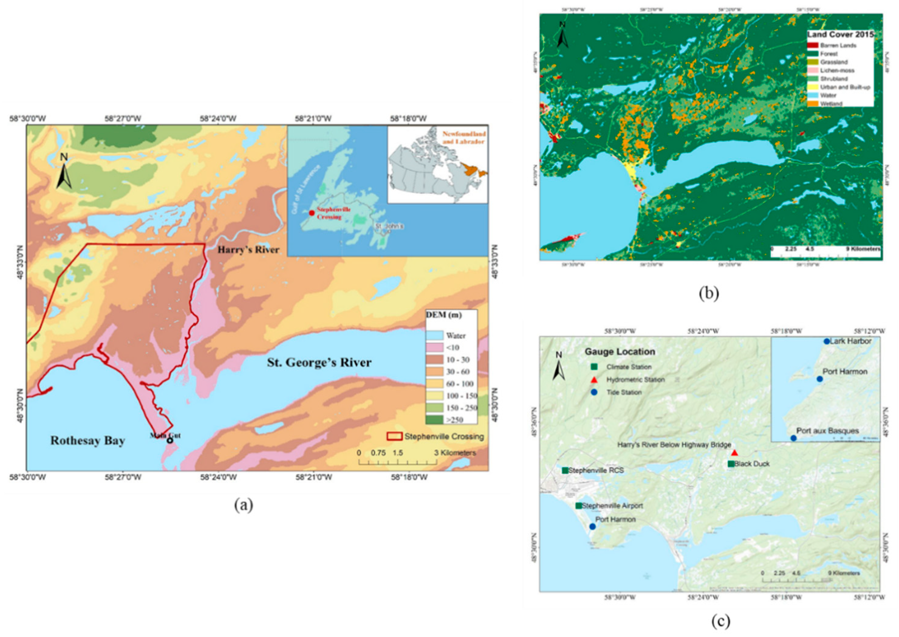
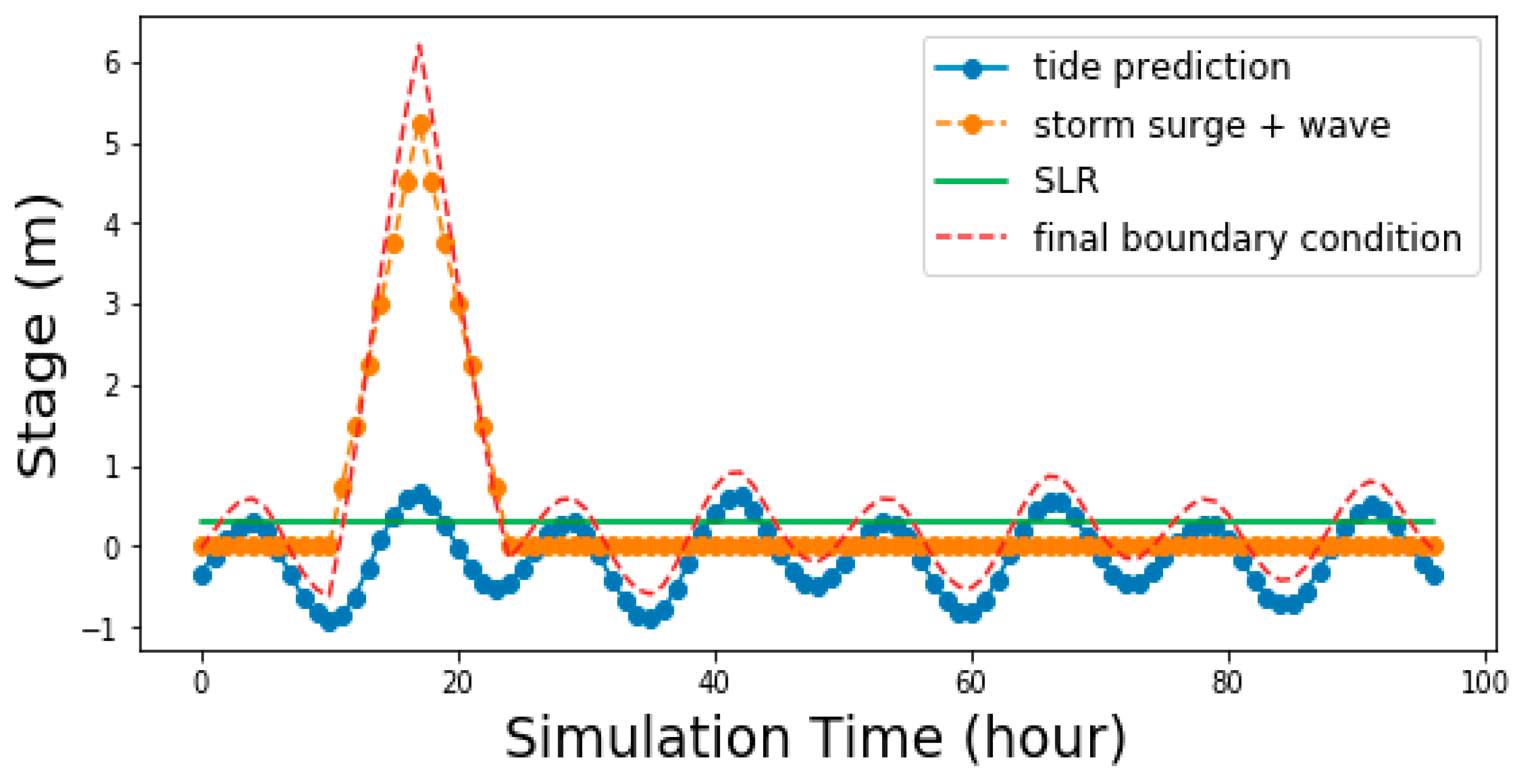
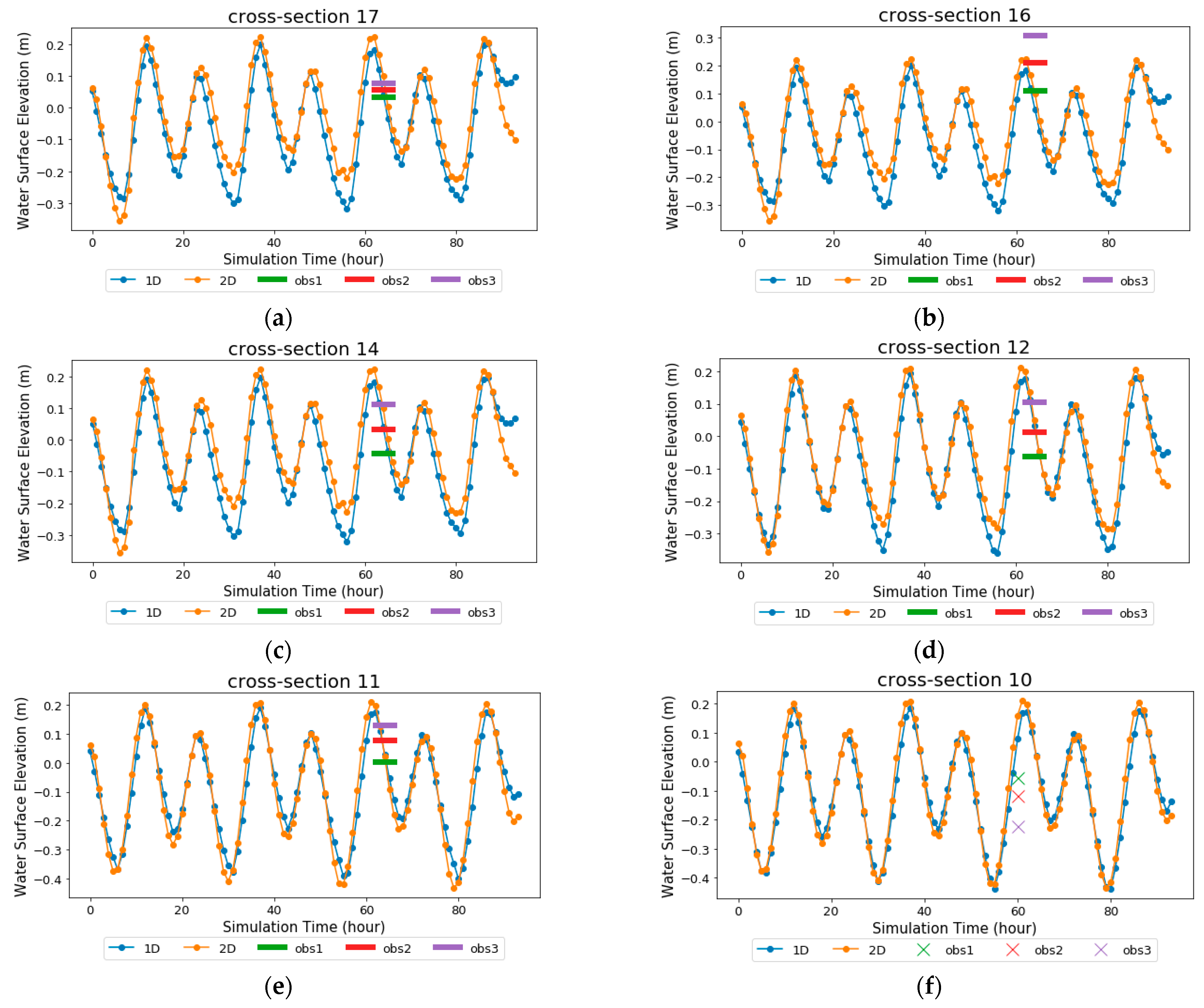
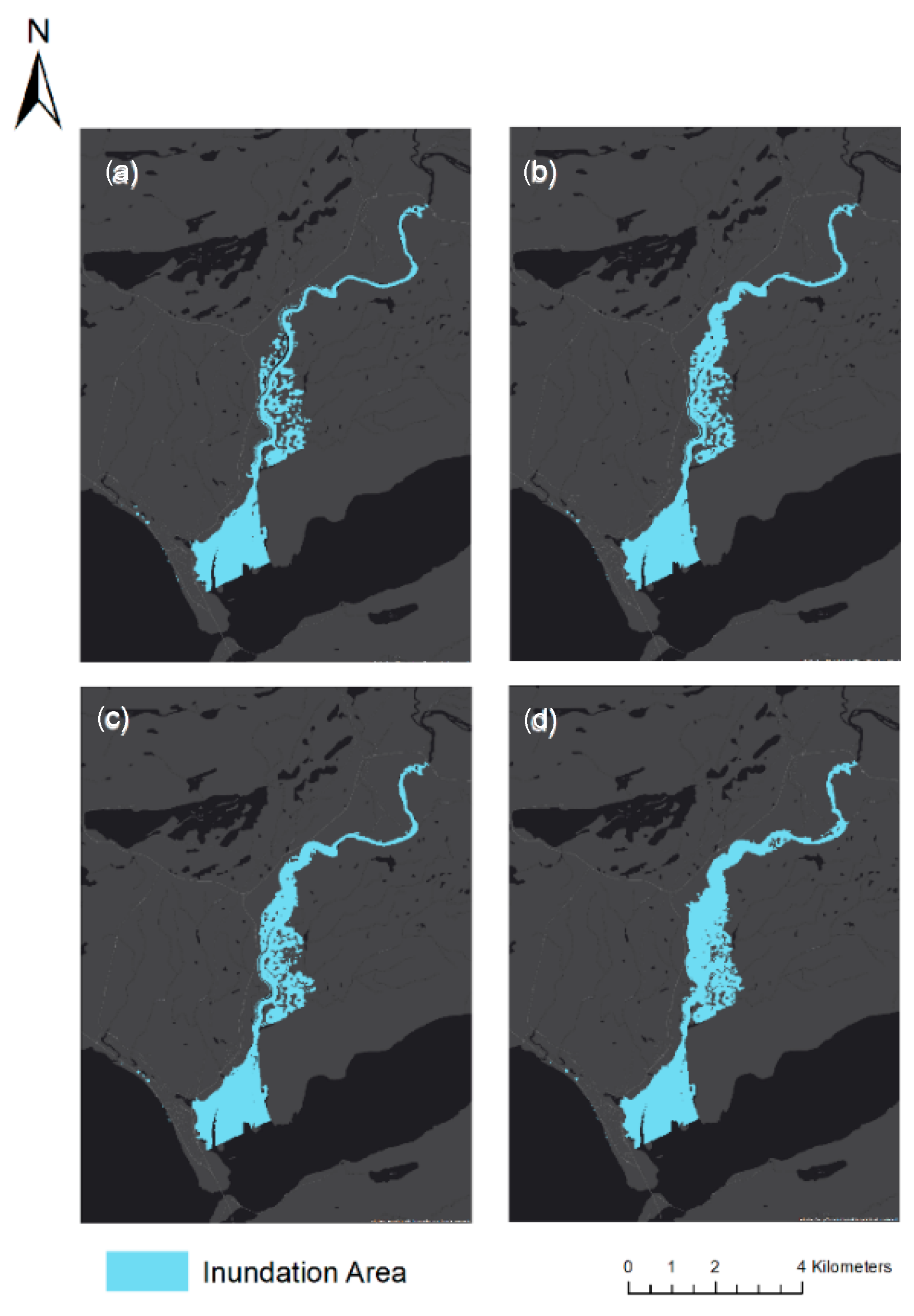
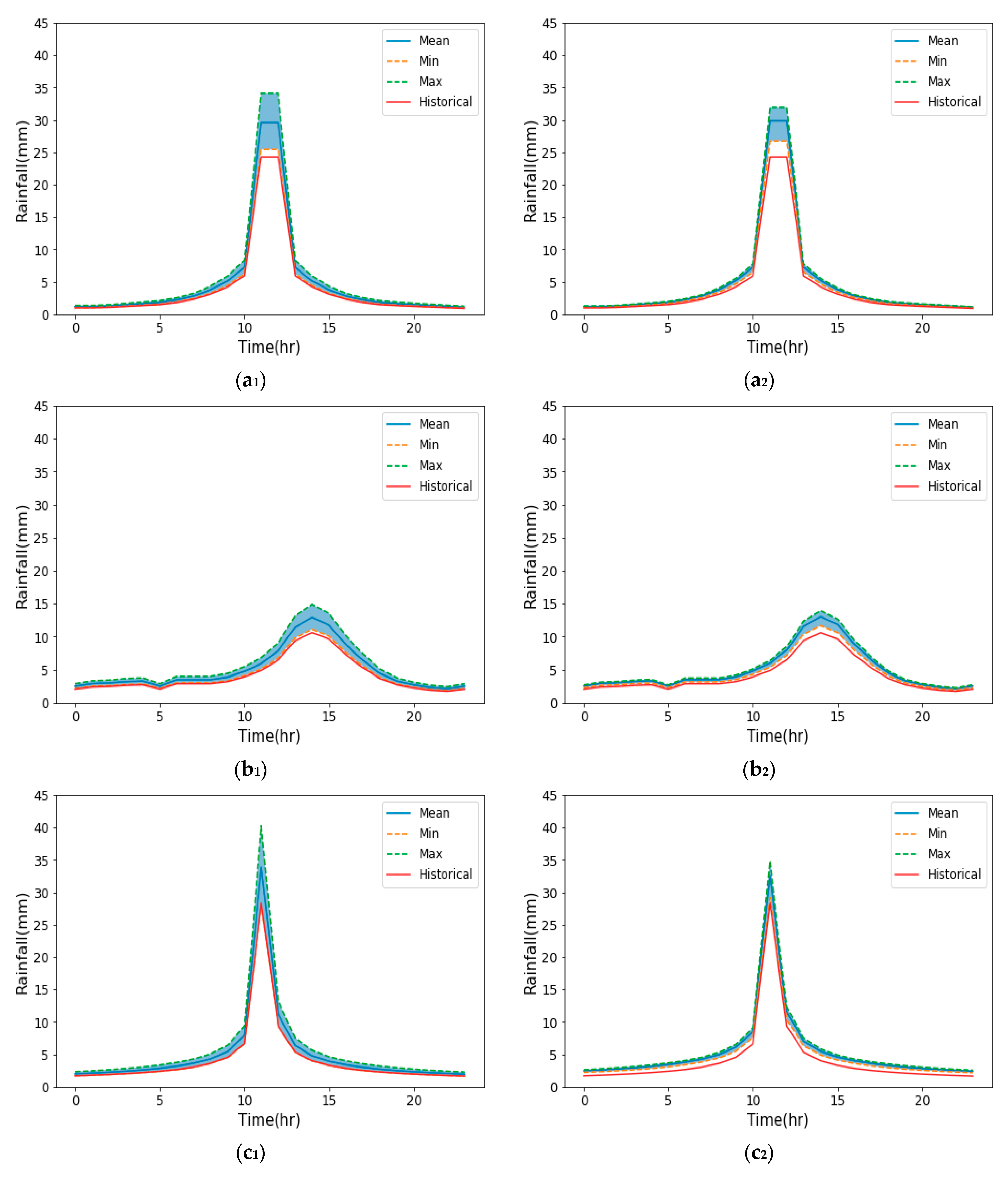
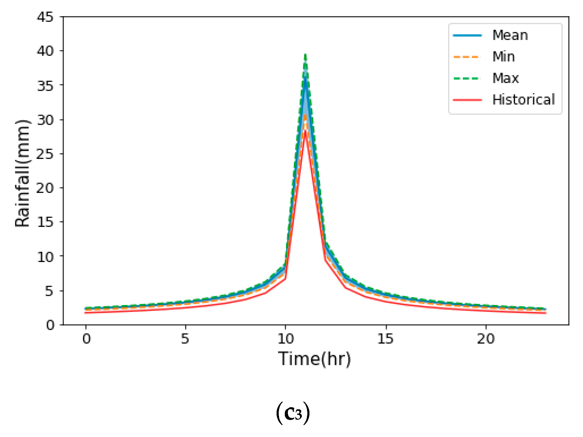
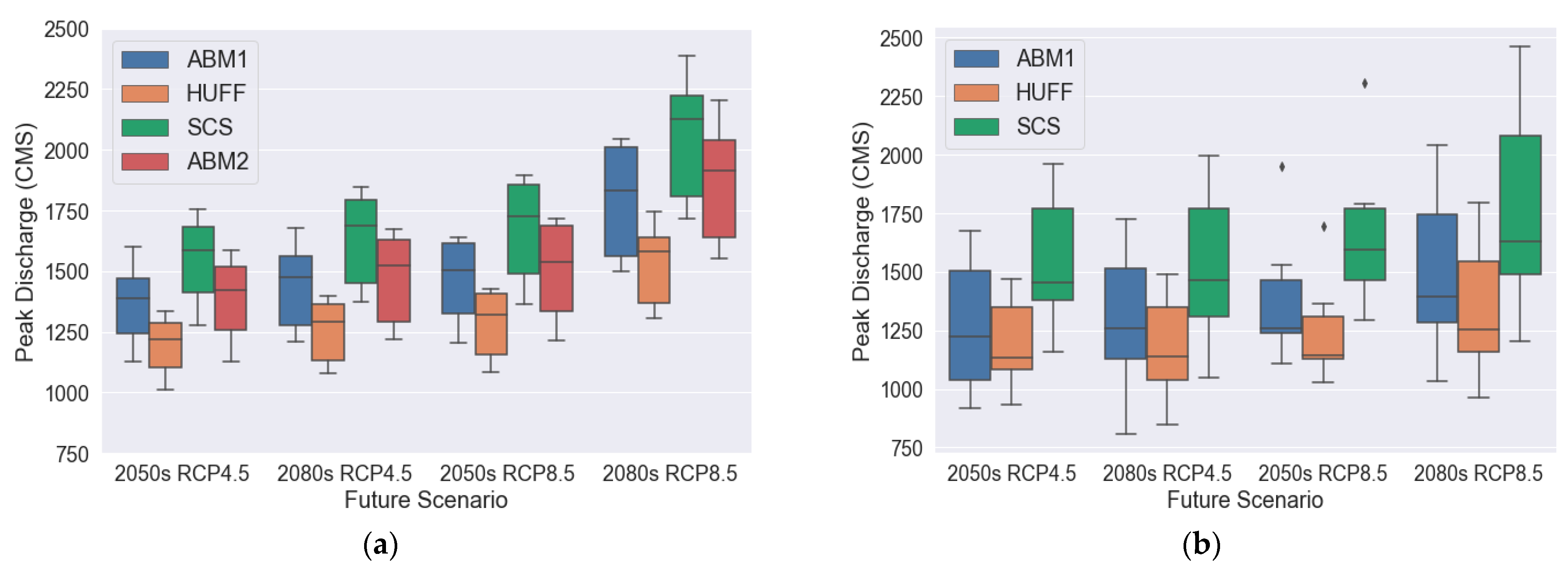
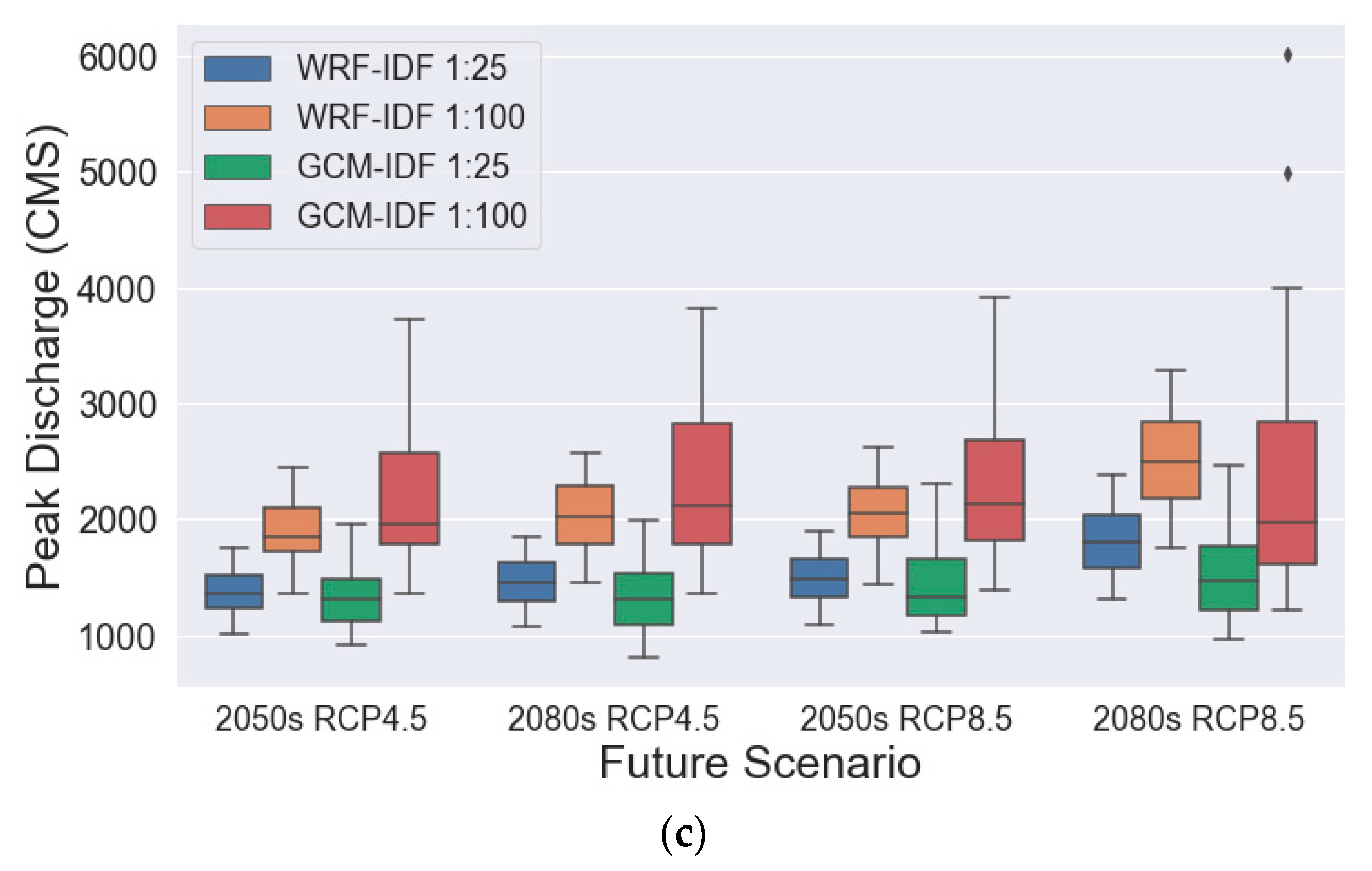
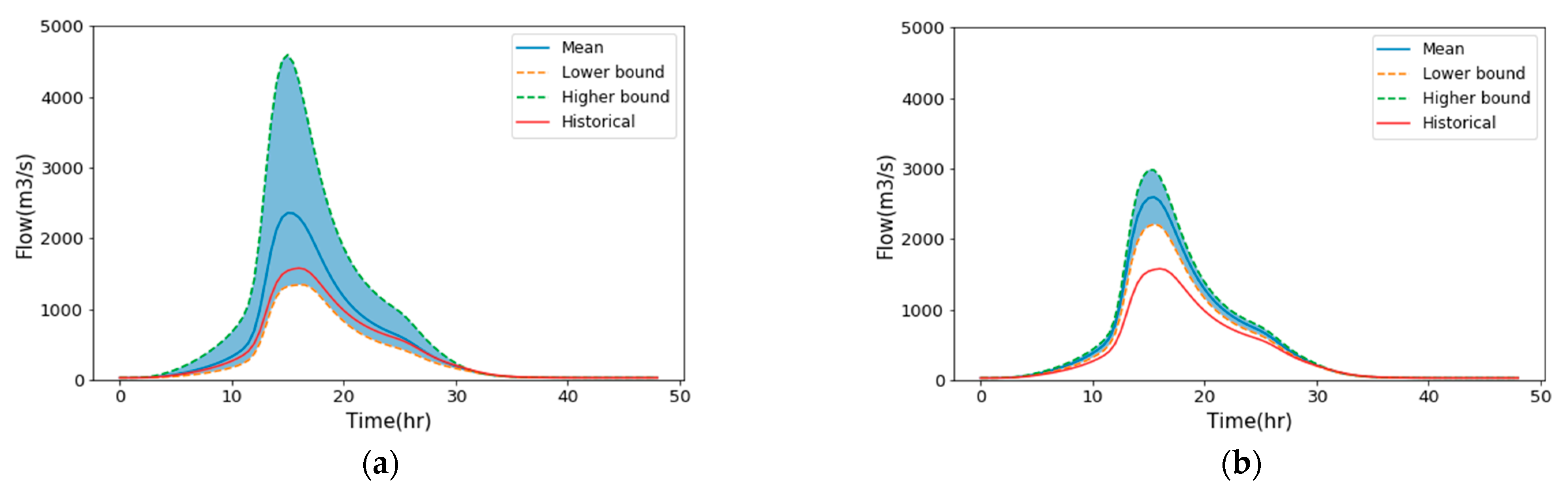
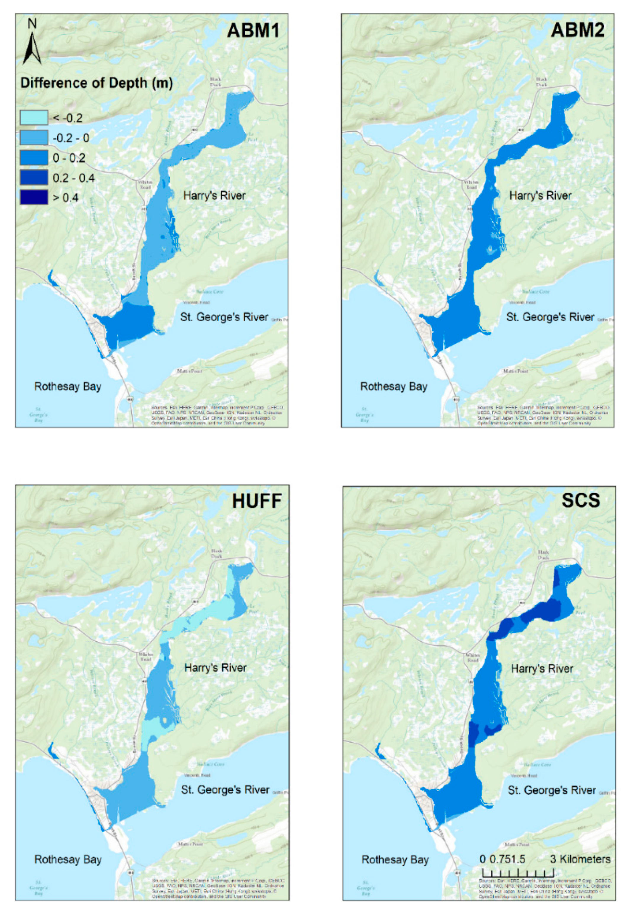
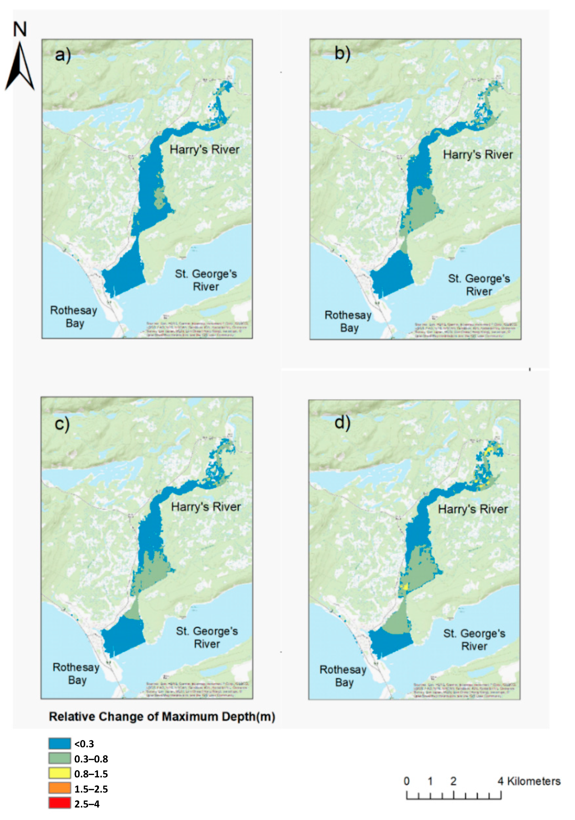
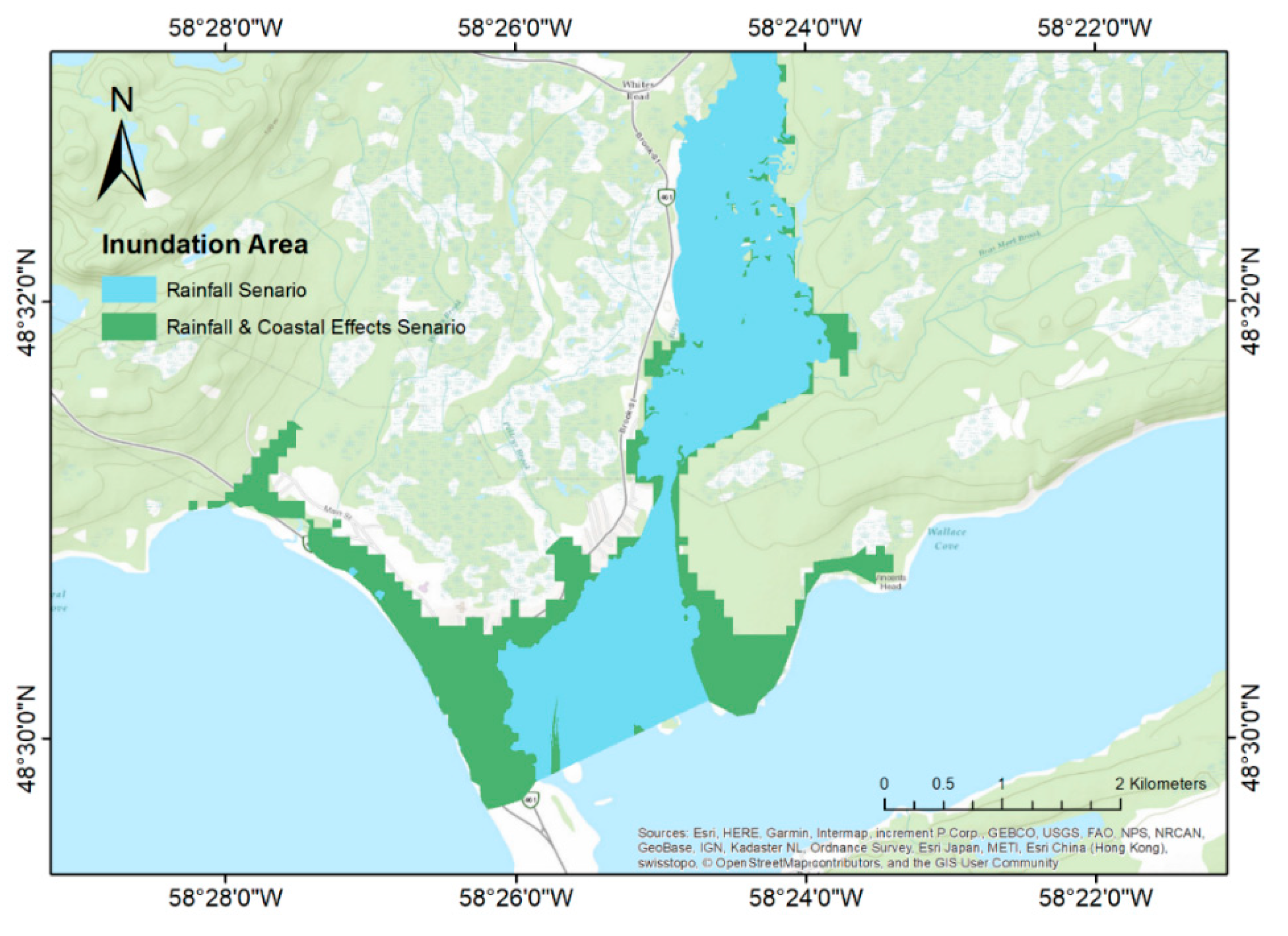
Table 1.
The components considered in coastal flood assessments under climate change.
| Coastal Components | Scenarios | |
|---|---|---|
| Storm surge and wave (m) | 25-year event | 100-year event |
| 5.25 | 6.34 | |
| Sea-level rise (m) | 2050s period | 2080s period |
| 0.3 | 0.8 | |
Table 2.
Comparison of 24 h rainfall (mm) amounts generated based on WRF- and GCM-IDF curves based on six GCMs.
Table 2.
Comparison of 24 h rainfall (mm) amounts generated based on WRF- and GCM-IDF curves based on six GCMs.
| Return Period (Years) | Historical (mm) | Future (mm) | |||
|---|---|---|---|---|---|
| Period | RCP | The Multi-Model Ensemble Average of GCMs (Minimum and Maximum) | |||
| GCM-IDF | WRF-IDF | ||||
| 25 | 107.94 | 2050s | 4.5 | 131.44 (111.38, 152.31) | 137.17 (121.80, 147.35) |
| 8.5 | 135.75 (118.8, 169.00) | 143.03 (126.65, 154.14) | |||
| 2080s | 4.5 | 129.93 (105.00, 153.94) | 141.62 (127.04, 151.94) | ||
| 8.5 | 142.50 (113.86, 176.36) | 163.05 (145.5, 176.54) | |||
| 100 | 142.79 | 2050s | 4.5 | 184.82 (144.33, 233.31) | 169.73 (150.15, 182.70) |
| 8.5 | 185.32 (149.58, 241.31) | 177.20 (156.33, 191.35) | |||
| 2080s | 4.5 | 181.76 (124.37, 237.56) | 175.40 (156.83, 188.55) | ||
| 8.5 | 200.00 (133.85, 333.34) | 202.70 (180.34, 219.89) | |||
Table 3.
Inundation area (square kilometers) for different design storms in the historical period.
| Design Storm | 25-Year Event | Difference from Huff Method | 100-Year Event | Difference from Huff Method |
|---|---|---|---|---|
| ABM | 6.221 | 0.057 | 6.427 | 0.178 |
| SCS method | 6.21 | 0.046 | 6.431 | 0.182 |
| Huff method | 6.164 | 0 | 6.249 | 0 |
Table 4.
Projected flood inundation extents (square meter) based on WRF-IDF curves (multi-model means of six GCMs).
Table 4.
Projected flood inundation extents (square meter) based on WRF-IDF curves (multi-model means of six GCMs).
| Return Level | RCP | Future Period | Fluvial Flood Scenario | Compound Flood Scenario |
|---|---|---|---|---|
| Mean | Mean | |||
| 25-year event | 4.5 | 2050s | 6.16 | 6.66 |
| 2080s | 6.29 | 6.87 | ||
| 8.5 | 2050s | 6.28 | 6.75 | |
| 2080s | 6.78 | 7.3 | ||
| 100-year event | 4.5 | 2050s | 6.97 | 7.63 |
| 2080s | 7.88 | 8.7 | ||
| 8.5 | 2050s | 7.81 | 8.49 | |
| 2080s | 8.98 | 9.78 |
Publisher’s Note: MDPI stays neutral with regard to jurisdictional claims in published maps and institutional affiliations. |
© 2021 by the authors. Licensee MDPI, Basel, Switzerland. This article is an open access article distributed under the terms and conditions of the Creative Commons Attribution (CC BY) license (https://creativecommons.org/licenses/by/4.0/).
Share and Cite
MDPI and ACS Style
Wang, S.; Najafi, M.R.; Cannon, A.J.; Khan, A.A. Uncertainties in Riverine and Coastal Flood Impacts under Climate Change. Water 2021, 13, 1774. https://doi.org/10.3390/w13131774
AMA Style
Wang S, Najafi MR, Cannon AJ, Khan AA. Uncertainties in Riverine and Coastal Flood Impacts under Climate Change. Water. 2021; 13(13):1774. https://doi.org/10.3390/w13131774
Chicago/Turabian StyleWang, Shuyi, Mohammad Reza Najafi, Alex J. Cannon, and Amir Ali Khan. 2021. "Uncertainties in Riverine and Coastal Flood Impacts under Climate Change" Water 13, no. 13: 1774. https://doi.org/10.3390/w13131774
Note that from the first issue of 2016, this journal uses article numbers instead of page numbers. See further details here.