Developing a Novel Water Quality Prediction Model for a South African Aquaculture Farm

Abstract

Providing an accurate prediction of water quality parameters for improved water quality management is a topical issue in the aquaculture industry. Conventional prediction methods have shown different challenges like a poor generalization, poor prediction accuracy, and high time complexity. Aiming at these challenges, a novel hybrid prediction model with ensemble empirical mode decomposition (EEMD) and deep learning (DL) long-short term memory (LSTM) neural network is proposed in this paper. In this innovative hybrid EEMD-DL-LSTM model, firstly, the integrity of the datasets is enhanced by applying moving average filtering and linear interpolation techniques of water quality parameter datasets pre-treatment. Secondly, the measured real sensor water quality parameters dataset is decomposed with the aid of the EEMD algorithm into disparate IMFs and a corresponding residual item. Thirdly, a multi-feature selection process is applied to make a careful selection of a strongly correlated group of IMFs with the measured real water quality parameter datasets and integrate them as inputs to the DL-LSTM neural network. The presented model is built on water quality sensor data collected from an Abalone farm in South Africa. The performance of the novel hybrid prediction model is validated by comparing the results against the real datasets. To measure the overall accuracy of the novel hybrid prediction model, different statistical indices, namely the Mean Absolute Error (MAE), Mean Square Error (MSE), Root Mean Square Error (RMSE), and Mean Absolute Percentage Error (MAPE), are used.

1. Introduction

In traditional aquaculture farming, the experienced aquafarmers’ observation and empirical judgment were sufficient to indicate and predict issues related to farm health. This form of management using tacit knowledge is gradually getting impractical for two main reasons—the number of experienced farmers is reducing, and the scale of the farms is growing. Hence, it is getting pertinent to use machine learning tools to understand and predict such issues in a timely manner. One aspect is monitoring the fluctuations of water quality parameters, e.g., dissolved oxygen, pH, temperature, salinity, etc., that are known to adversely affect the aquaculture environment. In some cases, even slight variations above or below the normal, optimal water quality parameter conditions may lead to physiological stress on the aquatic life, which can impact their feeding, breeding and increases susceptibility to diseases [1,2].

In recent years, the application of various machine learning techniques and methods has been explored for developing water quality parameters prediction models [3,4,5,6]. As a result, these models have become topical research hotspots in the field of aquaculture and water engineering. Presently, research studies in the field of water quality forecasting are mainly focusing on enhancing the applicability and accuracy of these predictive models using emerging technologies. To this end, varieties of new technologies, namely statistical analysis tools, Neuro-Fuzzy Inference System (ANFIS), machine learning, and artificial neural networks (ANNs), are being researched for the improvement of water quality parameters prediction models [7,8,9]. Some studies have adjudged artificial neural networks as the most preferred and reliable technique for the development of water quality parameters forecasting models because of their impressive suitability to irregular and nonlinear situations. As an example, Sheng et al. [10] and Chen et al. [11] conducted studies on a back-propagation (BP) neural network (NN), which is a typical representative of ANNs, and demonstrated that its enhanced algorithms have effective applicability to water quality parameters forecasting with obvious merits in forecasting nonlinear problems. Another variation, the radial-basis function (RBF) NNs, which has also been broadly applied in aquaculture, offers the advantage of a simplistic structure, the ability to globally approximate arbitrary functions with precision, and fast training speed [11,12,13,14].

However, the ANNs used by Chen et al. [11], which include BPNN and RBFNN, have the weakness of a long-term dependency problem. Research has shown that DL long-short term memory (LSTM) NN can overcome the above-mentioned weakness and can provide efficient applicability and reliability for water quality parameter prediction [1]. Additionally, combining the ensemble empirical mode decomposition (EEMD) method with DL-LSTM NN has demonstrated clear advantages over traditional LSTM NNs in terms of improved water quality parameter prediction accuracy in the aquaculture environment [1]. In this paper, a unique hybrid EEMD-DL-LSTM NN-based water quality parameters prediction model is proposed that overcomes the above-identified shortfalls in the literature [11,12,13,14].

The major approaches for water quality parameters prediction include the grey system theory technique, support vector regression machine technique, Markov technique, and time-series technique [13,14,15,16,17,18]. However, these widely applied approaches have certain drawbacks, which include the weak generalization problem, limited computational efficiency, and poor, unreliable forecasting accuracy. Consequently, these traditional approaches can hardly meet the growing requirements of precision aquaculture.

In recent years, different models have been proposed for water quality parameters forecasting in the aquaculture environment based on ANN and DL [17,19,20,21]. Some of these prediction models have applied a BP neural network approach in combination with different activation functions, such as tansig, logsig, and purelin, to develop a water quality forecasting model in aquaculture. Wijayanti [20] proposed a short-term prediction model based on a smooth support vector machine (SSVM) for aquaculture water quality management. Similarly, a water quality forecasting model for smart mariculture that applied a deep learning bi-directional stacked simple recurrent unit (Bi-S-SRU) network has been proposed in [21]. Many other prominent studies on water quality parameters forecasting models based on DL-LSTM have also been carried out [22,23]. The advantages of these prediction models include high fault tolerance, robustness, and good fitting of complex non-linear relations. However, they all share a common disadvantage because they use single-scale characteristics of the data for model training, thereby obtaining only the surface features of the datasets.

However, multi-scale prediction techniques have been shown to obtain more than single-scale features for the predicted signals by applying a decomposition method to the original signal [24,25]. Through the decomposition process, each sub-sequence of the original signal can reveal the signal’s distinct intrinsic features. The empirical mode decomposition (EMD) technique has widely been used for decomposing original signals into their intrinsic multi-scale features [26]. Forecasting techniques based on multi-scale characteristics of the original signal have been predominantly applied in various fields, such as wind power prediction [27,28], traffic flow forecasting [29,30,31], and rainfall prediction [32]. In the field of the aquaculture industry, Li et al. [24] used the EEMD technique to propose a hybrid prediction model based on the multi-scale features of the original signal to improve the prediction accuracy of Dissolved Oxygen (DO) concentration in a fishpond. Results of the proposed hybrid prediction model demonstrate the advantage of an EEMD method for predicting DO content in intensive aquafarming. The review of these related studies shows that hybrid prediction models based on multi-scale characteristics of the real data are suitable for water quality parameter prediction in the aquaculture industry. Hence, this paper proposes a novel hybrid EEMD-DL-LSTM NN-based water quality parameters prediction model for the aquaculture industry through the combination of an EEMD technique with DL-LSTM NN.

Although the hybrid prediction model proposed in [24] is similar to the novel hybrid EEMD-DL-LSTM NN-based water quality parameters prediction model proposed in this paper, their study adopted the least squares support vector regression (LSSVR) and BPNN. However, in theory, a linear system can be solved by LSSVR, but solving a large dataset becomes impractical due to its high computational complexity, thereby limiting the merits of adopting LSSVRs in large-scale applications. Similarly, the long-term dependency problem associated with BPNN and RBFNN makes our proposed novel hybrid EEMD-DL-LSTM prediction model a unique solution because LSTM can overcome this problem.

2. Methods and Materials

2.1. Study Area Description and Datasets Analysis

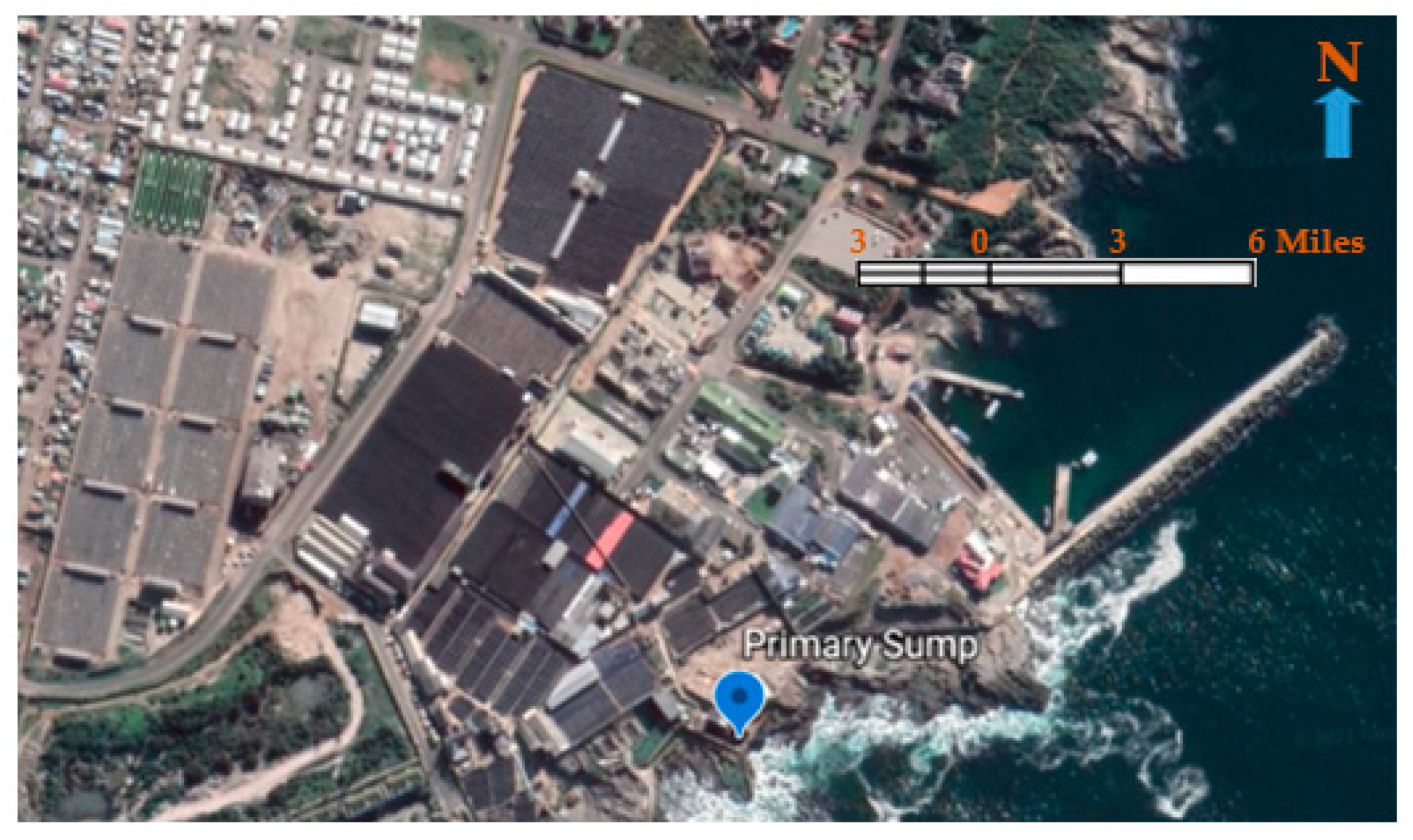
Abagold Limited is a South African abalone (Haliotis midae) hatchery, grow-out, and processing facility situated in the New Harbour of Hermanus, South Africa. Characterized by injections of the warm Agulhus current and cold Benguela current, Walker Bay is prone to frequent upwelling of cold, nutrient-rich water in the summer months (November–March) interjected by warm water events. Historically, this has resulted in algal blooms, which can affect the production of aquaculture facilities. The farm is a land-based, flow-through system housing some 650 tons. Data was collected via Xylem WTW IQ Sensor Net probes [33], situated in the primary and secondary sumps distributing incoming seawater to the farming platforms (see Figure 1).

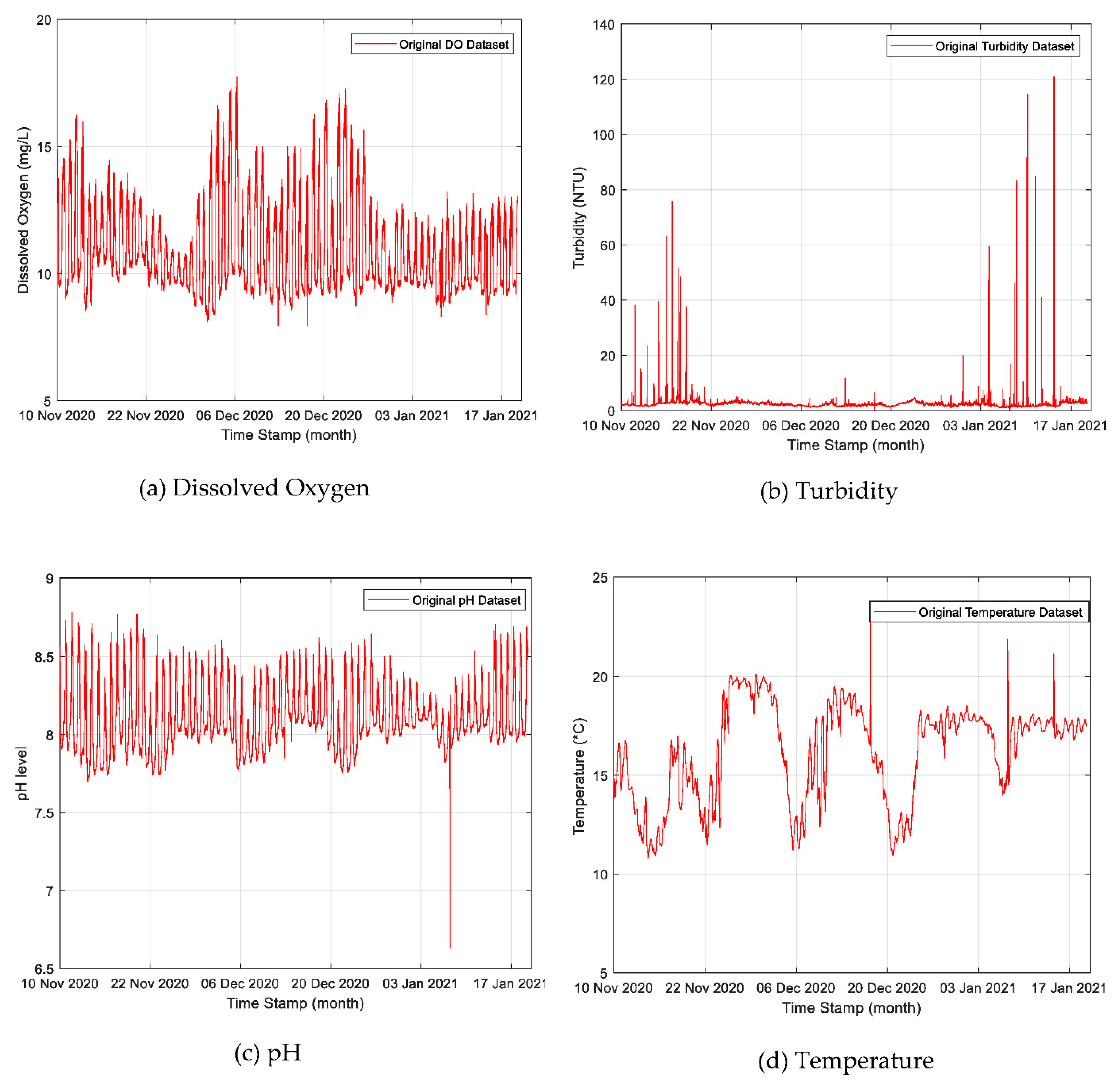
A total of 20,730 sets of non-linear and non-stationary water quality parameters time-series data were collected at Abagold between November 2020 and January 2021. The water quality parameters included dissolved oxygen, turbidity, temperature, and pH. The collected datasets are shown plotted as line graphs in Figure 2a–d. The trend variations of DO (mg/L), turbidity (NTU), pH (m/L), and temperature (°C) are shown in Figure 2a–d between November 2020 and January 2021.

2.2. Data Filling and Correction

Non-linear and non-stationary water quality parameters time-series dataset defects usually result in an excessive deviation between the measured original water quality parameters values and the prediction results. The basis of an accurate time-series analysis and the development of effective and reliable predictive models is high-quality sample data. To provide a concise, accurate dataset for the prediction model and improve prediction accuracy, the measured water quality parameters data were pre-processed, as discussed below. Generally, the issue of missing data is inevitable with automatic water quality monitoring systems. The water quality parameters such as dissolved oxygen, turbidity, pH, and temperature were automatically measured throughout the day at 5-minute intervals. To fill in any missing data, the filling-in approach, called a linear interpolation algorithm [34], was applied to achieve a better estimation effect that can accurately approximate the missing data values. In data analysis, the linear interpolation algorithm took the ratio of two known data points and one unknown data point as a linear relationship. Therefore, to obtain the missing, unknown water quality parameter value, the linear interpolation technique applied the slope of the presumed line to compute the time-series dataset increment. Hence, the data set was completed.

Definition 1. 

The nature of the measured parameters.

An installed automated freshwater monitoring system at the Abagold measures time-series water quality factors at a constant time interval everyday which can be denoted as $\beta$, then $n$ length time-series of the measured water quality factors datasets is defined as (1)

$$S_{i,n}=\left\{\left(X_{i, 1},T_1\right),\left(X_{i, 2},T_2\right), \cdots ,\left(X_{i, n},T_n\right)\right\}$$

(1)

where $X_{i, l}$ represents the value of the measured ith time-series water quality factor by the automatic sensory monitoring system at time $T_l$ $\left(1\le i\le \beta , 1\le l\le n\right)$, and at other given $T_l$, the time interval is constant at $\Delta T=\left(T_{l+1}-T_l\right)=5$ min. Therefore, if the original value $X_{i, l}$ is missing, its estimated value ${\widehat{X}}_{i, l}$ can be obtained with the problem of minimum, which is given as $\left|{\widehat{X}}_{i, l}-X_{i, l}\right|$ changed into the missing value estimation problem. Based on the measured data $X_{i, x}$ and $X_{i, y}$ at time $T_{i, x}$ and $T_{i, y}$, respectively, the linear imputation function $L\left(t\right)$ could be formulated for the time-series water quality parameters monitoring systems as:

$$L\left(t\right)=X_{i, x}+\left(\frac{X_{i, x}-X_{i, y}}{T_{i, x}-T_{i, y}}\right)·\left(t-T_{i, x}\right).$$

(2)

For any missing time-series water quality parameters data at any given moment, the linear interpolation algorithm firstly finds the two closest moments $T_{i, x}$ and $T_{i, y}$ $\left(T_{i, x}<t<T_{i, y}\right)$, and estimates the lost data value at time $t$ with the help of the known measured data $X_{i, x}$ and $X_{i, y}$ of $T_{i, x}$ and $T_{i, y}$ moments based on Equation (2), i.e., ${\widehat{X}}_n=L\left(t\right)$.

2.3. Data Correlation Analysis

This study applied the Pearson’s correlation coefficient technique to analyze the existing correlations between the measured time-series water quality parameters such as dissolved oxygen, turbidity, water pH, and temperature to the Abagold aquaculture farm. To better understand the existing correlations between two variables, the Pearson’s correlation coefficient technique [35] has been widely used as a data analyzing technique, which is also described as the quotient of co-variance and standard deviation between two variables. The Pearson’s correlation coefficient system was used after cleaning and pre-processing the sensor-measured time-series water quality factors, to analyze the existing correlations between the required parameters.

Table 1. Data correlation analysis results.

	Dissolved Oxygen	Turbidity	pH	Temperature
Dissolved Oxygen	1	−0.09677	0.54826	−0.14893
Turbidity	−0.09677	1	−0.03914	−0.05654
pH	0.54826	−0.03914	1	0.55366
Temperature	−0.14893	−0.05654	0.55366	1

contains the correlations among the measured water quality parameters obtained through data analysis and calculations. Table 1 shows that the dissolved oxygen has an extremely strong negative correlation with turbidity but maintains a moderate strong positive correlation with water pH, and a strong negative correlation with temperature. Dissolved oxygen and turbidity are inversely related because the upward or downward variation of one affects the other in the opposite direction. Regarding the literature value for such a type of correlation, when there is a high level of turbidity in an aquaculture water body, it means there would be less dissolved oxygen for living organisms to breath effectively [36]. Therefore, if the turbidity increases to a certain unhealthy level, the fishes would start getting stressed and sick due to an obvious lack of dissolved oxygen, which can lead to fish death, thereby negatively affecting aquatic life populations.

Additionally, it was shown that the water temperature shares a moderately strong positive correlation with water pH. Finally, it is also shown in Table 1 that turbidity has a very strong negative correlation with the pH and water temperature. This means that a high level of turbidity increased the overall aquaculture water body temperature since suspended particles tend to absorb more heat. Therefore, these factors led to a reduction in dissolved oxygen.

3. Prediction Model Design

The proposed prediction model comprises two-stage processes to improve the overall accuracy and minimize the error margin of the water quality parameters prediction results. The first stage of the two processes applies the EEMD technique to decompose the time-series dataset into a series of disparate intrinsic mode functions (IMFs) and uses a multi-feature selection process to select a set of strongly correlated IMFs that aid towards enhancing the absorption features. In the second stage, the selected set of strongly correlated IMFs are integrated into inputs for the DL-LSTM neural network. The implementation processes of the EEMD approach and DL-LSTM NN are presented in Section 3.1 and Section 3.2, respectively.

3.1. EEMD Method

The EMD technique [37] is a self-adaptive, non-linear data signal decomposition approach, which decomposes the time-series datasets into separate IMFs and a corresponding residual item by the use of a recursive process with each distinct time-scale feature. The time-series signal $x\left(t\right)$ is decomposed via a unique sifting process [38] into distinct $n$ units of $Z_i$ IMFs and ensemble the $R_n$ trend as expressed in (3).

$$x\left(t\right)={\displaystyle \sum }_{i=1}^n{Z}_i+R_n$$

(3)

Each of the corresponding outcomes of the decomposition process ($n$ units of $Z_i$ IMFs) generally maintain high orthogonality to one another, with each IMF representing a special range of frequency and energy. Therefore, the summation of all the separate $n$ units of $Z_i$ IMFs is usually equal to the measured original water quality parameters datasets. According to Rilling et al. [39], each of the resultant IMFs must meet two conditions, namely:

(1)

The total number of extrema and the zero-crossings of IMFs must be equal or, at most, differ by one.

(2)

The mean of local minima and local maxima envelopes is zero at any point.

Admittedly, the nature of the original time-series datasets signal $x\left(t\right)$ does not always meet the definition of the IMFs because a vast part of the original datasets consists of disparate frequencies. Hence, to ensure that $x\left(t\right)$ satisfies the definition of the IMFs, the EMD method applies the sifting process. The application of the sifting process helps in the aspect of:

(1)

Ride waves identification and eradication, and

(2)

IMFs’ wave profiles refining to obtain more symmetric wave profiles.

Finally, the procedures of the applied datasets signal $x\left(t\right)$ decomposition method are summarized as shown below:

(a)

Determine all the extrema of the signal $x\left(t\right)$.

(b)

Apply the linear interpolation technique between minima (respectively, maxima) with envelopes, $e_{min}\left(t\right)\left\{\mathrm{resp}.e_{max}\left(t\right) \right\}$.

(c)

Compute the mean of the envelopes ${\widehat{m}}_j\left(t\right)=\frac{\left\{e_{min}\left(t\right)+e_{max}\left(t\right)\right\}}{2}$, with $j$ representing the number of iterations.

(d)

Then, extract the detail $Z_i=x\left(t\right)-{\widehat{m}}_j\left(t\right)$.

(e)

Repeat step (a) to step (d) until the IMFs converged with $Z_i\left(t\right)$ satisfy the definition of the IMFs.

(f)

Repeat step (a) to step (e) to determine the residual $R_n\left(t\right)$, with $R_n\left(t\right)=x\left(t\right)-Z_n\left(t\right)$.

In accordance with the stopping criteria [39], the sifting process aids the refining of the above procedure by repeating step (a) to step (d) on the signal $R\left(t\right)$ till it has a zero-mean. The result of the signal decomposition can only be considered as an effective IMF once the zero mean is achieved. Subsequently, the corresponding residual $R_n\left(t\right)$ of the signal is generated by applying step (f).

During the sifting process, the use of the stopping criterion ensures that the generated IMFs via the EMD decomposition method meet the acceptable IMF conditions given above. The stopping criterion is implemented through standard deviation $\left(\sigma \right)$ size reduction by sifting the results twice as expressed in (4).

$$\sigma ={\displaystyle \sum }_{t=0}^T\left[\frac{{\left|Z_{i-1}\left(t\right)-Z_i\left(t\right)\right|}^2}{Z_{i-1}^2\left(t\right)}\right]$$

(4)

The acceptable value of $\sigma$ is typically within the range of 0.2 and 0.3 [1]. In practice, the sifting process is terminated automatically once the computed $\sigma$ value lies within the acceptable range of 0.2 and 0.3.

Despite the significant contributions of the EMD method in different applications, its ability in handling signal processing problems remains insufficient due to its strong dependence on the signals’ frequencies and amplitudes, as well as their differences. The ensemble EMD (EEMD) method is a refined form of EMD, which can improve the efficiency of the signal decomposition process and overcome the inherent shortcomings of mode mixing [1], which is generally associated with the traditional EMD method. With the EEMD method, before the decomposition of signals, a uniformly distributed Gaussian white noise is added to limit the adverse effect of the mode-mixing problem of the conventional EMD method [40]. With the aid of this process, the EEMD algorithm is able to overcome both the challenges of multi-dimensional computation and mode mixing [41].

In the EEMD method, the amplitude and the ensemble number of the added Gaussian white-noise $W_i\left(t\right)$ are predetermined and initialized. Firstly, disparate uniformly distributed Gaussian white noise $W_i\left(t\right)$ with the same amplitude in accordance with the number of data signals within the ensemble will be introduced to the original water quality parameters signal $x\left(t\right)$ by $M$ times to generate $M$ different modified signals $x_i\left(t\right)$, as shown in (5).

$$x_i\left(t\right)=x\left(t\right)+W_i\left(t\right);i=1,2,3,\cdots , M$$

(5)

Secondly, the conventional EMD method decomposition process is performed on each of the modified signals $x_i\left(t\right)$. For instance, if the modified signal’s decomposition generates separate $n$ units of $Z_i$ IMFs and a corresponding residue item as a trend, then applying the EEMD approach would generate $M \times n$ IMF signals with distinct $n$ trends $R_{in}\left(t\right)$. Therefore, $x_i\left(t\right)$ can be rewritten as shown in (6).

$$x_i\left(t\right)={\displaystyle \sum }_{j=1}^n{Z}_{ij}\left(t\right)+R_{in}\left(t\right);i=1,2,3,\cdots , M$$

(6)

Furthermore, the EEMD method resolves the mode mixing problem by averaging the resulting IMF set $F_j\left(t\right)$ and the derived residue trend $R\left(t\right)$.

$$F_j\left(t\right)=\frac{1}{M}{\displaystyle \sum }_{i=1}^M{Z}_{ij}\left(t\right);i=1,2,3,\cdots , n$$

(7)

$$R\left(t\right)=\frac{1}{M}{\displaystyle \sum }_{i=1}^M{R}_{in}\left(t\right)$$

(8)

For large amounts of datasets, the error ${\delta }_n$ incurred during the decomposition process due to the addition of the uniformly distributed Gaussian white noise can be obtained via the empirical formula in (9)

$${\delta }_n=\frac{\omega }{\sqrt{K}}$$

(9)

where ${\delta }_n$ represents the final standard deviation, $\omega$ denotes the amplitude of the applied uniformly distributed white noise, and $K$ represents the total number of ensembles. Then, using the above empirical formula, $W_i\left(t\right)$ can be given by (10) as:

$$W_i\left(t\right)=\omega \times noise\left(t\right)$$

(10)

The original water quality parameters time-series datasets are effectively decomposed by the EEMD technique into $n$ ensemble mode functions and one corresponding ensemble residual item. For every frequency band, the disparate mode function components that are contained within the band are uniquely dissimilar and can vary according to variation of the water quality parameters time-series dataset $x\left(t\right)$. Similarly, the derived ensemble residual item indicates the original data signal $x\left(t\right)$ trend.

3.2. DL-LSTM Neural Networks

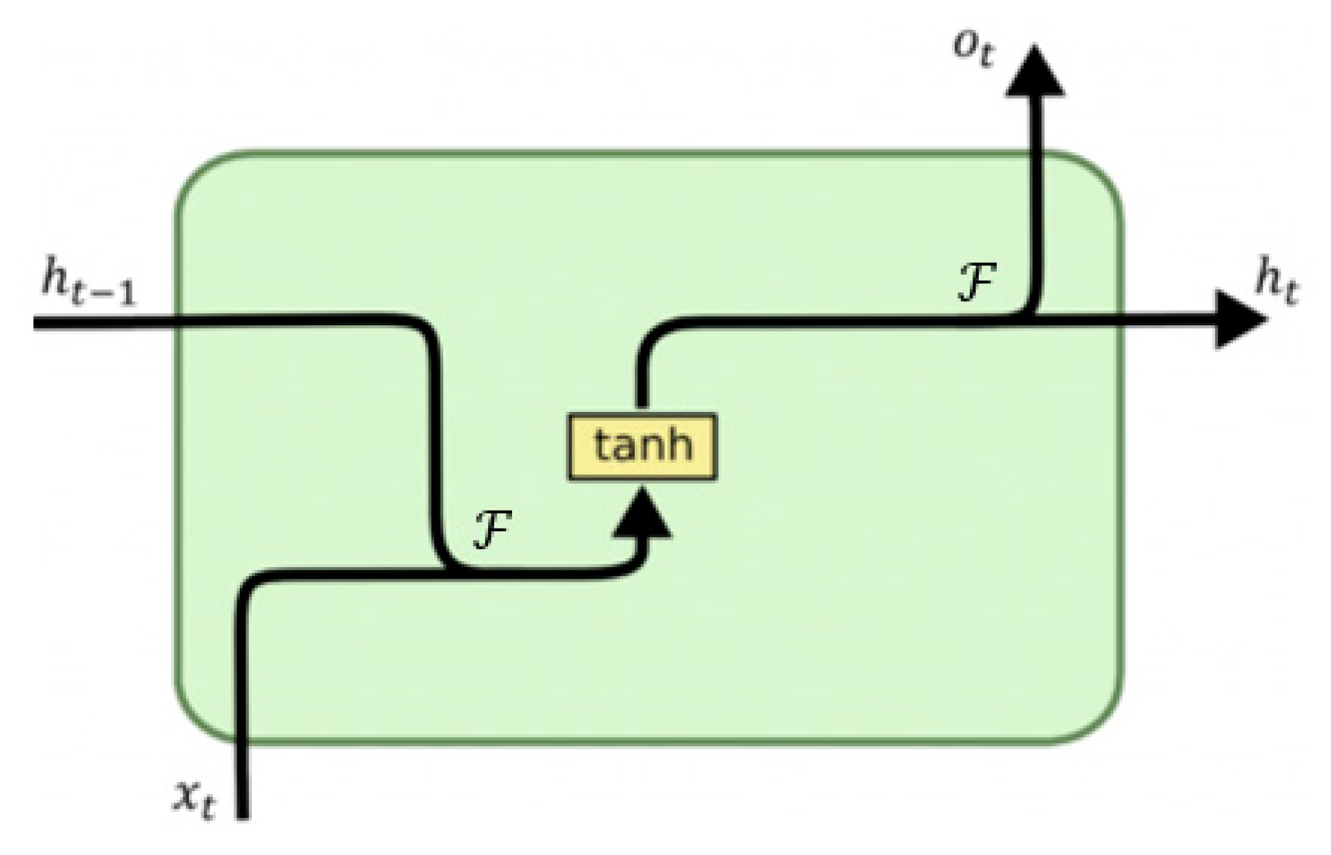
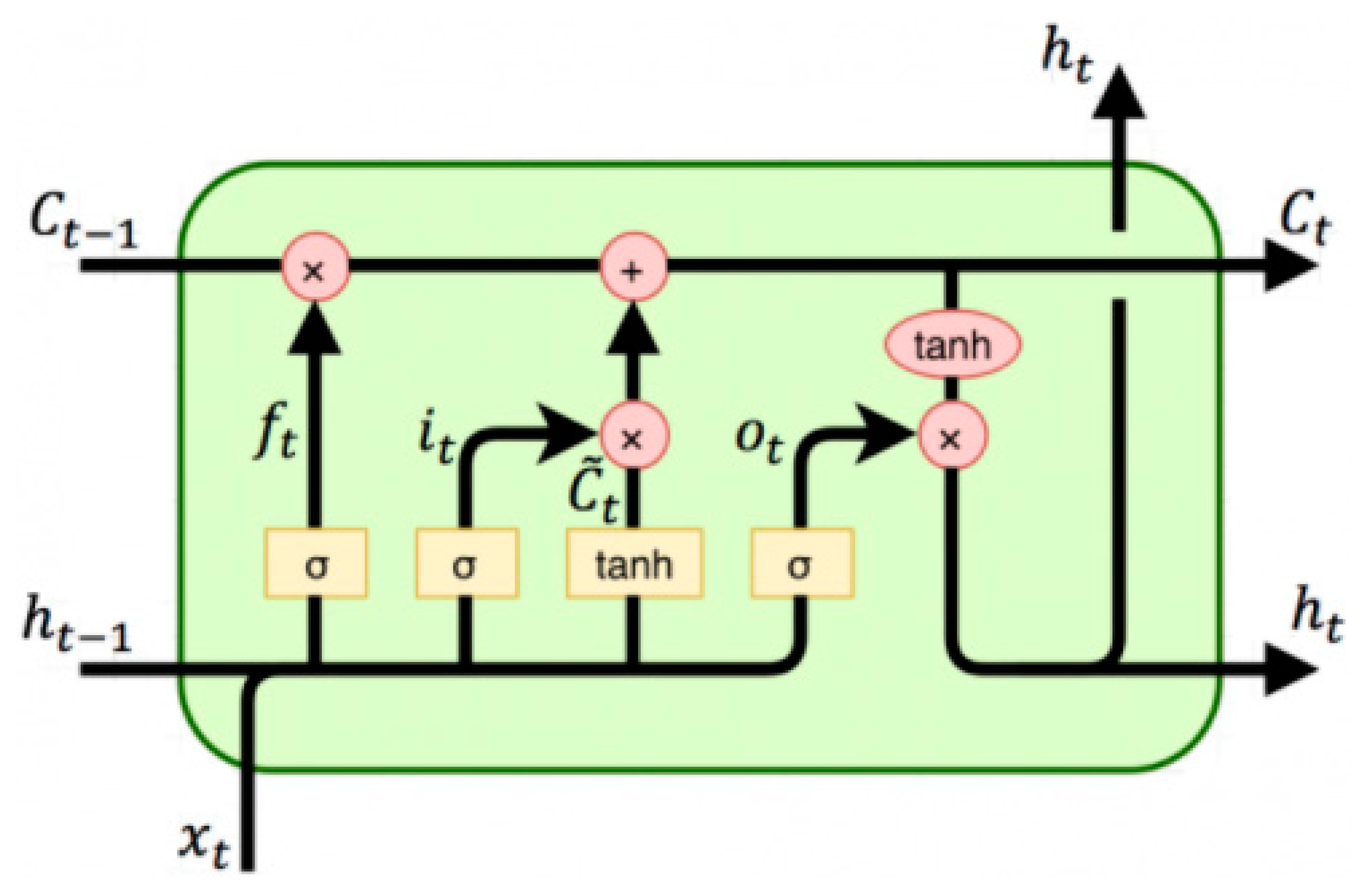
DL-LSTM NNs [22,23,42] are a special type of recurrent NN (RNN) with a significant improvement and the ability to learn long-term dependencies, which gives it an advantage over other artificial NNs such as BPNN, RBFNN, etc. Figure 3 illustrates a typical schematic diagram of a traditional RNN node with the previous hidden state represented by $h_{t-1}$, activation function by $ℱ$, current input sample by $X_t$, current output by $y_t$, and the current hidden state by $h_t$. As depicted in Figure 3, all RNNs generally have the form of chain repeating modules of NNs. These repeating modules generally have a very basic structure in standard RNNs, like a single tanh layer only. However, DL-LSTM, which stores information with the aid of purpose-built memory cells, maintains a similar chain-like structure but with a different structured repeating module (see Figure 4). As illustrated in Figure 4, there are four distinct interacting layers in a DL-LSTM cell.

The equation below illustrates the calculation processes involved in DL-LSTM NNs.

(a) 

Forget gate equation:

$${ℱ}_t=\sigma \left(W_f\times \left[h_{t-1},x_t\right]+b_f\right)$$

(11)

where ${ℱ}_t$ denotes a vector with values ranging from 0 to 1, $b_f$ is the bias of the forget gate, $\sigma$ represents the logistic sigmoid function of the gate, and $W_f$ is the weight matrix of the gate. The sigmoid layer helps in determining whether new information is relevant for updating or irrelevant and discarded. Each relevant new information that passed through, is assigned a weight which ranges from −1 to 1 by tanh function to determine its level of importance. In both input and output gates, as shown (12) through (15) below, similar tanh function sigmoid layer operations are repeated.

(b) 

Input gate equations:

$$I_t=\sigma \left(W_i\times \left[h_{t-1},x_t\right]+b_i\right)$$

(12)

$${\tilde{C}}_t=\tan \mathrm{h}\left(W_i\times \left[h_{t-1},x_t\right]+b_i\right)$$

(13)

(c) 

Output gate equations:

$$O_t=\sigma \left(W_o\times \left[h_{t-1},x_t\right]+b_o\right)$$

(14)

$$h_t=O_t\times \tan \mathrm{h}\left(C_t\right)$$

(15)

(d) 

Cell state equation:

$$C_t=\left\{\left({ℱ}_t\times C_{t-1}\right)+\left(I_t\times {\tilde{C}}_t\right)\right\}$$

(16)

where $W_i$ and $W_o$ denote the weight matrices of the input gate and output gate, tanh is a hyperbolic tangent function, while $b_i$ and $b_o$ denote the network bias vectors.

3.3. Proposed Unique Hybrid EEMD-DL-LSTM NN-Based Water Quality Parameters Prediction Model

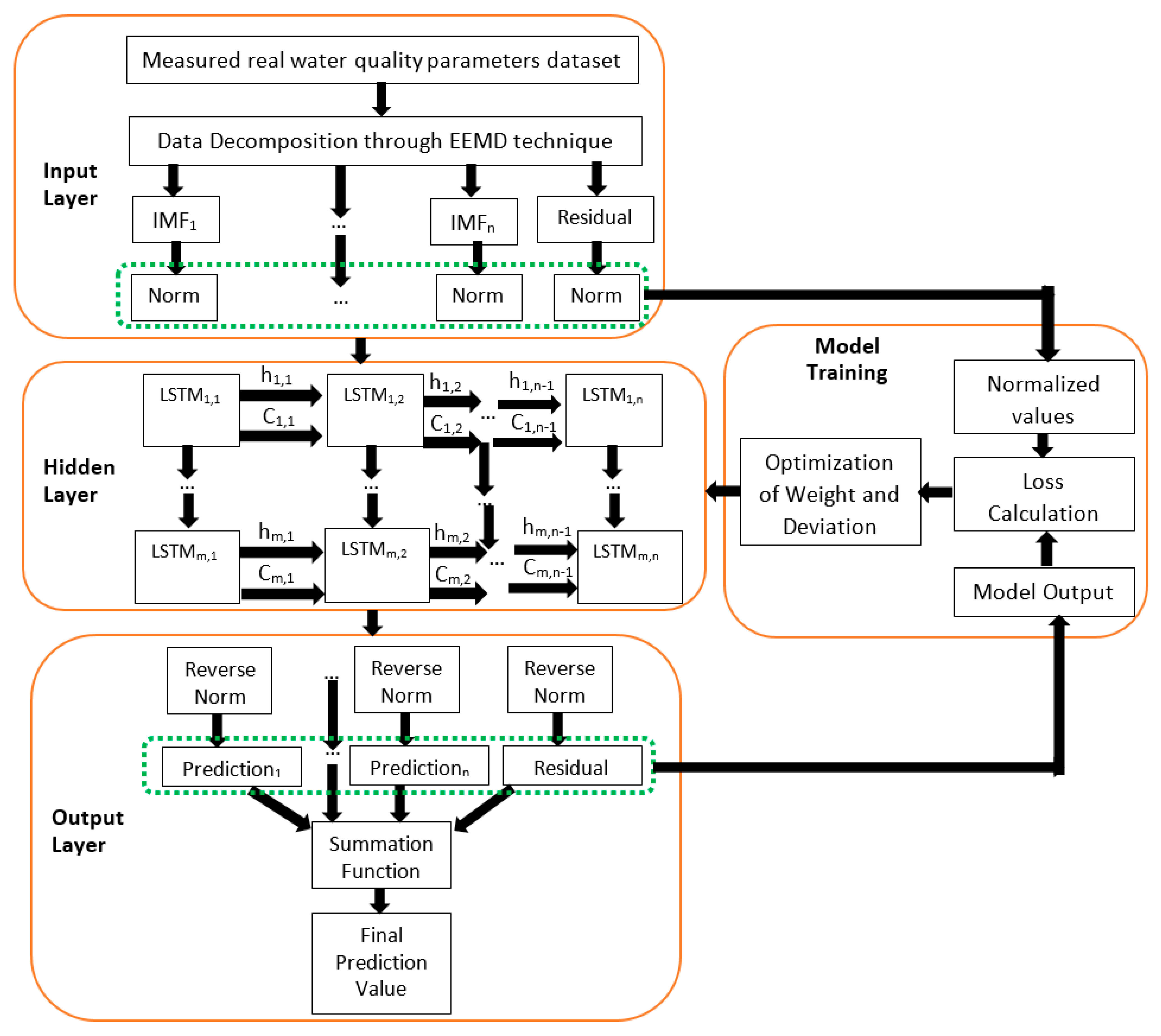
The proposed new hybrid prediction model is shown in Figure 5. With the novel hybrid model, measured real water quality parameters content datasets are decomposed through the EEMD algorithm into different components to increase the forecasting accuracy of the new model with a minimized error margin. The detailed step-by-step procedures demonstrated in Figure 5 show the three important key stages that precede the development of the novel hybrid EEMD-DL-LSTM NN-based water quality parameters prediction model. Under the first stage, the original signal decomposition method is applied to decompose the measured water quality parameters dataset $x\left(t\right)$ into various IMFs and the corresponding residual item $R_n\left(t\right)$ in the input layer of Figure 5. A unique iterative sifting process is used to perform the original signal $x\left(t\right)$ decomposition as expressed in $\left(17\right)$.

$$x\left(t\right)={\displaystyle \sum }_{i=1}^n{F}_i\left(t\right)+R_n\left(t\right)$$

(17)

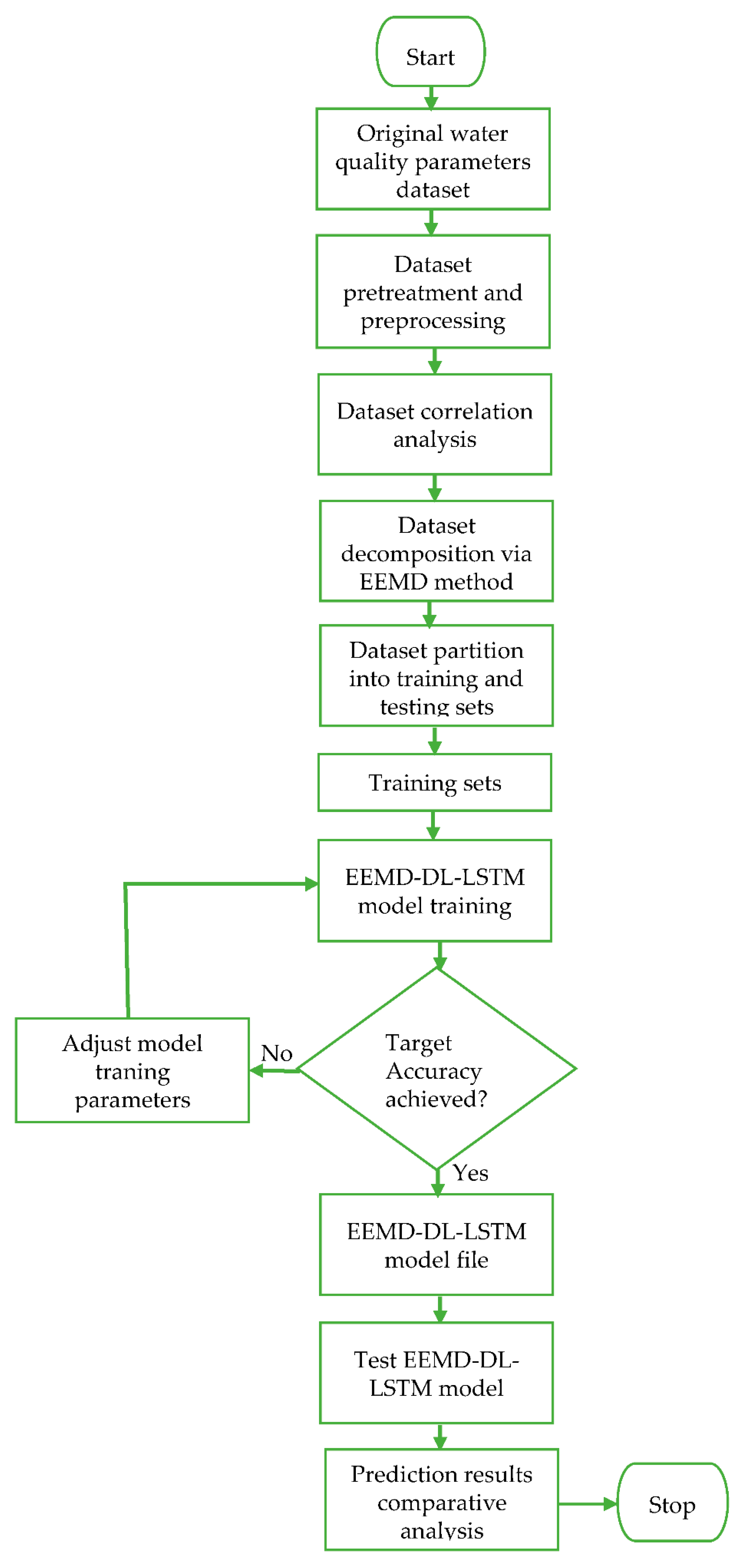
In the second stage, the different IMFs and the corresponding residual item $R_n\left(t\right)$ is utilized for the prediction by the DL-LSTM NN after normalization in the hidden layer of Figure 5. Lastly, a reverse normalization operation is performed on the individual prediction results of the DL-LSTM NN before efficiently combining all the individual prediction results together using a summation operation, with the aid of the summation function, to get the final predicted values, as shown in the output layer of Figure 5. As clearly illustrated using the extended novel hybrid model with manifold hidden DL-LSTM layers (LSTM_1,1, LSTM_1,2, …, LSTM_m,1, up to LSTM_m,n) in Figure 5, individual hidden layers of the stacked DL-LSTM is equipped with various memory cells thereby, earning the proposed prediction model the term deep learning NN method [42]. The flowchart in Figure 6 demonstrates the entire proposed water quality parameters prediction process.

4. Performance Evaluation Metrics

For the evaluation of the hybrid EEMD-DL-LSTM NN-based water quality parameters prediction model, four performance evaluation metrics were introduced to evaluate its prediction accuracy. The metrics are described as shown below:

Definition 2. 

MAE measures the overall prediction accuracy for continuous time-series data. It is used to measure the average magnitude of the total incurred errors over a set of predictions without considering their direction. Error, in this case, refers to the difference between the original measured water quality parameters values and the predicted values for those parameters. During performance evaluation, it is usually applied as a reference to compare the merits and demerits. The formula of this evaluation metric is given as:

$$\mathrm{MAE}=\frac{1}{D}{\displaystyle \sum }_{i=1}^D\left|O_i-P_i\right|$$

(18)

Definition 3. 

MSE calculates the mean average of the squared prediction errors over all the instances in the test dataset and the formula given as:

$$\mathrm{MSE}=\frac{1}{D}{\displaystyle \sum }_{i=1}^D{\left(O_i-P_i\right)}^2$$

(19)

Definition 4. 

RMSE is a quadratic scoring principle that measures the average magnitude of the prediction error. It provides the mean prediction error that is rather more sensitive, especially to extreme original measured values. The resultant changes in the evaluation index can stand as the benchmark for the effectiveness and reliability test of the predictive model. The formula of RMSE is expressed as:

$$\mathrm{RMSE}=\sqrt{\frac{1}{D}{\displaystyle \sum }_{i=1}^D{\left(O_i-P_i\right)}^2}$$

(20)

Definition 5. 

MAPE is an evaluation metric that measures the size of the prediction error in percentage terms. It does not only measure the deviation between the original measured water quality parameters values and the forecasted values, but it also considers the ratio between the deviation and the original measured values. The formula of MAPE is given as:

$$\mathrm{MAPE}=\frac{1}{D}{\displaystyle \sum }_{i=1}^D\left|\frac{O_i-P_i}{V_i}\right|.$$

(21)

In (18), (19), (20), and (21) above, D represents the number of data points in the dataset, O_i and P_i denote the original measured water quality parameters values and the predicted values, respectively. The closer these four performance evaluation metrics tend towards 0, the higher the overall forecasting and fitting accuracy of the proposed hybrid model.

5. Results and Discussion

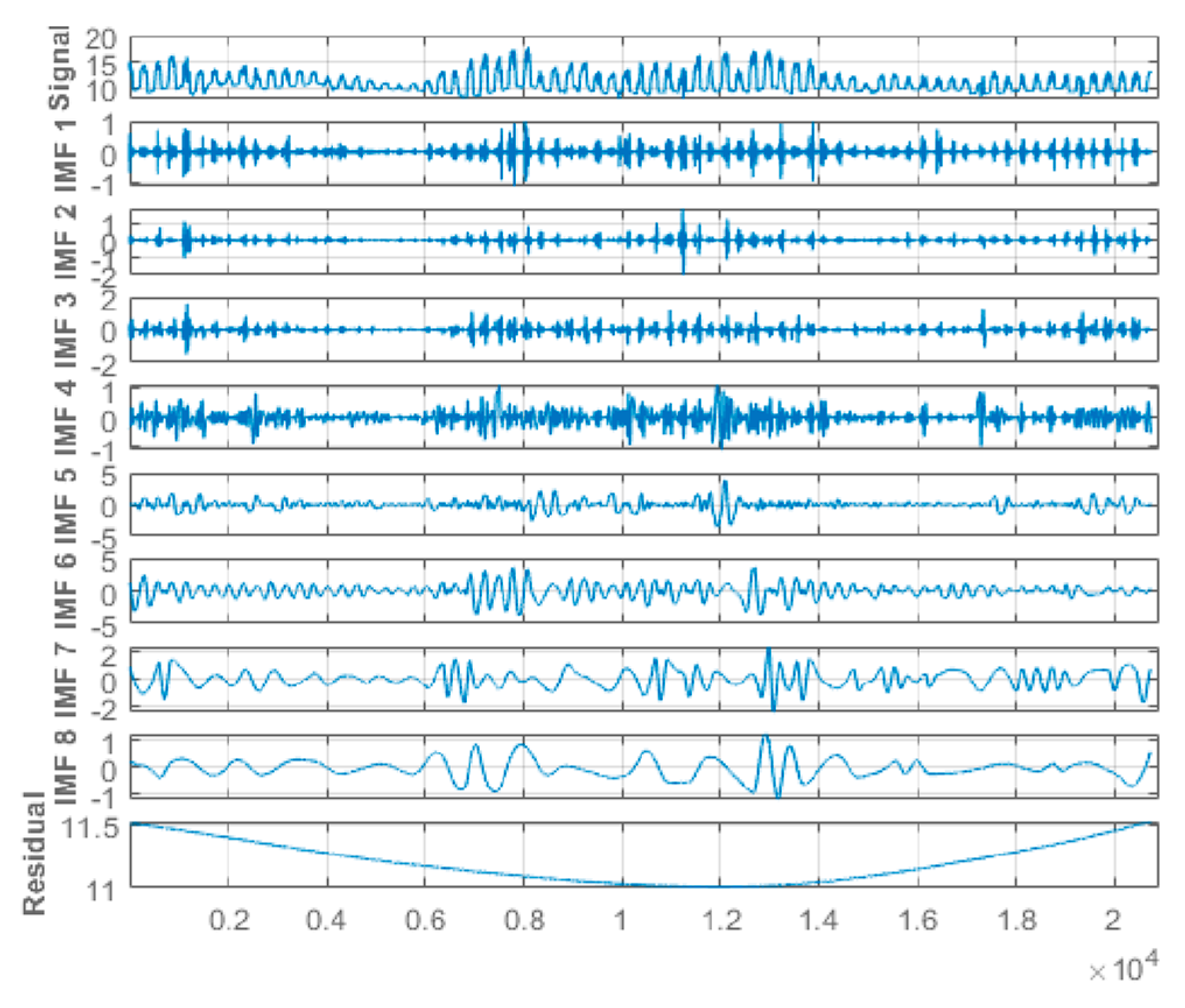
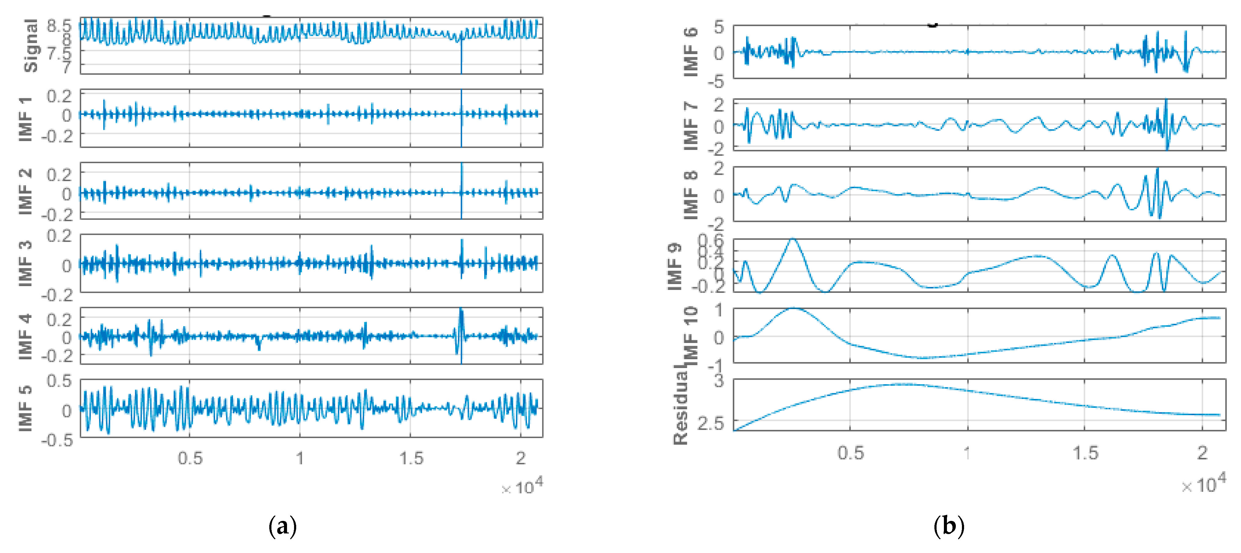
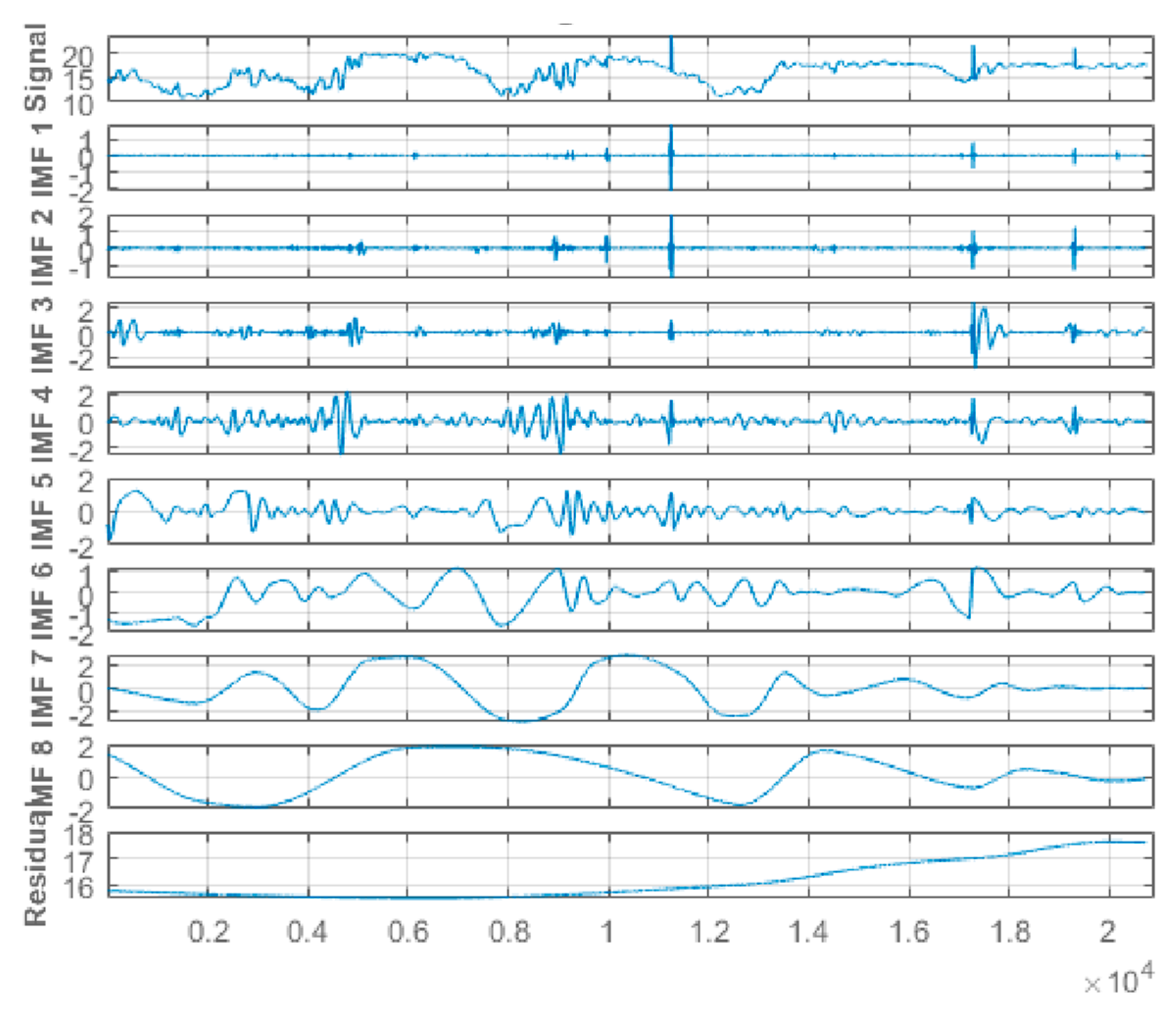
This study applied hourly centered moving average values to the original-measured water quality parameters time-series data from the Abagold Farm. Additionally, the EEMD technique, which is an effective and reliable approach for non-linear, non-stationary time-series signal decomposition, was applied for decomposing the water quality parameters datasets signals. Decomposing the water quality parameters dataset is an essential aspect of the proposed novel hybrid EEMD-DL-LSTM prediction model for predicting short-range values of the water quality parameters content. The original water quality parameters sensor data was decomposed through the application of the EEMD method into eight (8) different stable IMFs and a corresponding residue, as depicted in Figure 7, Figure 8, Figure 9 and Figure 10 for dissolved oxygen, turbidity, pH, and water temperature, respectively. For improved performance, the amplitude of the introduced white noise in the EEMD method was set to 0.2 [37]. Finally, the EEMD method extracted a set of sub-band signals, which were applied within the decomposition stage of the novel hybrid EEMD-DL-LSTM NN-based prediction model. A summation of the low-frequency IMFs was used to extract the EEMD trend.

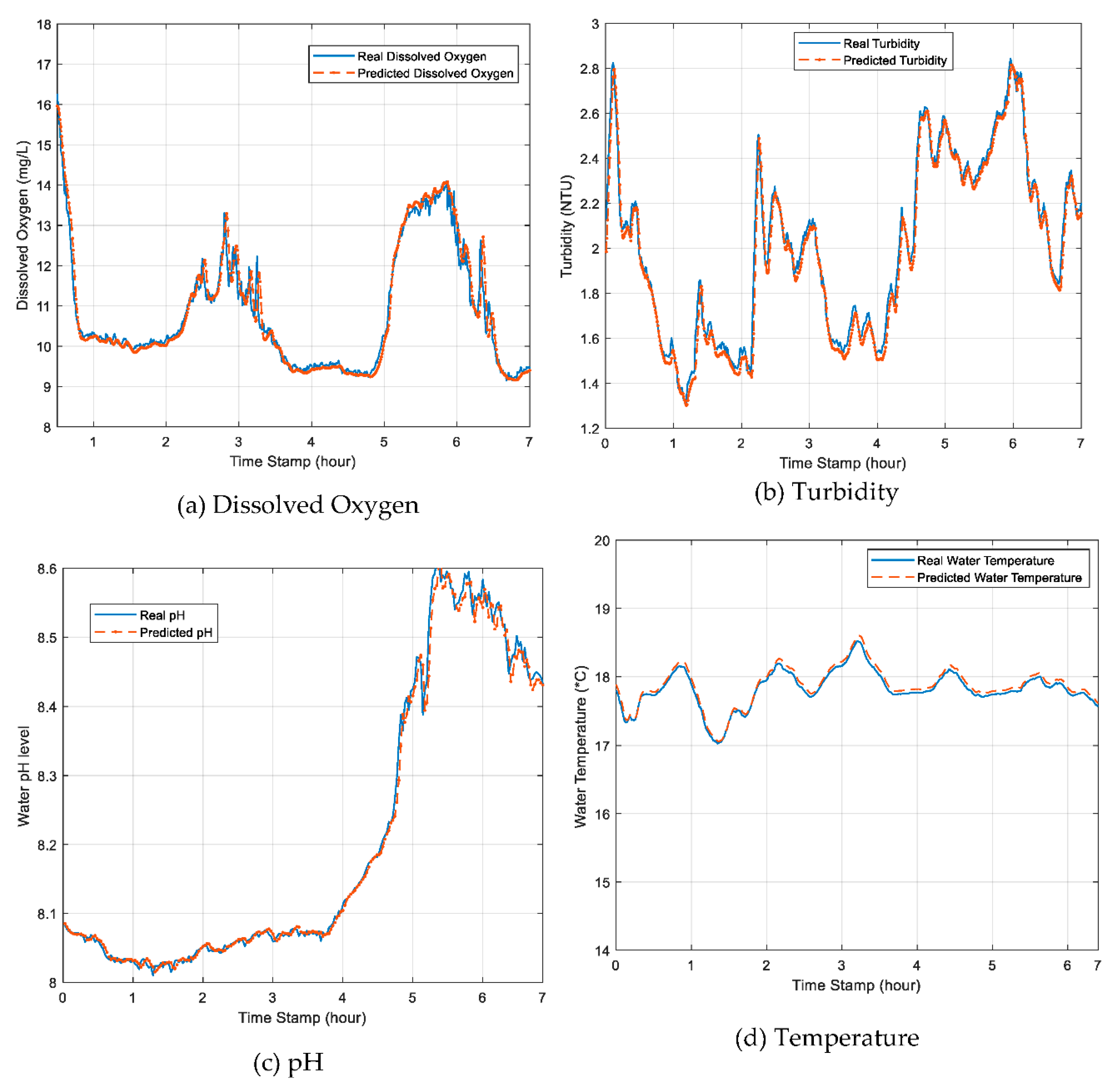
The novel hybrid EEMD-DL-LSTM prediction model used seventy-five percent (75%) of the pre-processed real water quality parameters dataset as a learning data sample (training dataset) as well as performed DL and carried out model training. The remaining twenty-five percent (25%) of the actual sensor monitoring water quality parameters data of 5th to 18th January 2021 was used as the test dataset. The predicted results were compared with the real monitored water quality parameters data. The set of measured real experimental water quality parameters datasets such as dissolved oxygen, turbidity, pH, and water temperature from the South African Abagold Farm indicated that the proposed novel hybrid prediction model yields valuable results and outperforms other similar water quality parameters prediction models in terms of high accuracy and low time cost. For the purpose of fair performance comparison, this study used the MAE, RMSE, and MAPE error evaluation methods for pH, temperature, dissolved oxygen, and turbidity in

Table 2. Comparison of prediction accuracy for individual water quality parameters against a similar model^x. Not applicable (NA) is used in this table because the reference model [2] did not include error statistics for DO and turbidity in their paper. ^x DL-LSTM model [2] and our proposed novel hybrid EEMD-DL-LSTM NN prediction model.

MAE								RMSE								MAPE
pH		Temperature		DO		Turbidity		pH		Temperature		DO		Turbidity		pH		Temperature		DO		Turbidity
DL-LSTM	EEMD-DL-LSTM	DL-LSTM	EEMD-DL-LSTM	DL-LSTM	EEMD-DL-LSTM	DL-LSTM	EEMD-DL-LSTM	DL-LSTM	EEMD-DL-LSTM	DL-LSTM	EEMD-DL-LSTM	DL-LSTM	EEMD-DL-LSTM	DL-LSTM	EEMD-DL-LSTM	DL-LSTM	EEMD-DL-LSTM	DL-LSTM	EEMD-DL-LSTM	DL-LSTM	EEMD-DL-LSTM	DL-LSTM	EEMD-DL-LSTM
0.0042	0.0140	0.0421	0.0251	NA	0.0262	NA	0.0309	0.6236	0.0407	0.0519	0.0325	NA	0.0355	NA	0.0291	0.0092	0.0074	0.0850	0.0073	NA	0.0075	NA	0.0078

; and run time(s), MAE, MSE, RMSE, and MAPE error evaluation methods for dissolved oxygen in

Table 3. Comparison of prediction accuracy and run time (s) against similar models *.

Statistical Evaluation Metrics	BP Model	SAE-BP Model	DL-LSTM Model	SAE-LSTM Model	EEMD-DL-LSTM Model
Run Time (s)	3.4000	9.1000	22.0000	28.2000	2.3700
MAE	0.3000	0.2580	0.1000	0.0690	0.0375
MSE	0.1352	0.0953	0.0166	0.0077	0.0024
RMSE	0.3680	0.3090	0.1290	0.0880	0.0489
MAPE	0.0310	0.0270	0.0100	0.0070	0.0072

* BP model, RBF model, LSTM model, LSTM and Sparse Auto-Encoder (SAE; SAE-LSTM), and SAE-BPNN prediction models are proposed in [23], and our proposed novel hybrid EEMD-DL-LSTM NN prediction model.

, which were the same error evaluation methods used in the reference models in [2,23], respectively. The overall prediction accuracy of the proposed model was highly improved with a minimized time complexity because of the multi-feature selection process carried out by the EEMD method to make a selection of the strongly correlated group of IMFs components with the measured real water quality parameter datasets and integrating them as inputs for the DL-LSTM neural network, unlike the related models that do not apply the EEMD method. Similarly, in Table 2, a comparison of prediction accuracy for individual water quality parameters against a similar model [2] is shown. The results, as depicted in Figure 11a–d, indicated that our proposed model could be very useful for deployment as an early warning system in an aquaculture environment. These impressive results further buttressed the importance of applying this model in aquaculture water quality management. Furthermore, the designed and development of a non-complex user-friendly graphical user interface (GUI) with menus and buttons can go a long way to enable aquafarmers, even in sub-urban locations, to apply the proposed model using a desktop computer with basic configuration and less technical hands-on training.

As shown in Figure 11a–d, it was concluded that the forecasted water quality parameters values had a good agreement with the real sensor monitored values from the aquafarm water, which indicated that the proposed novel hybrid EEMD-DL-LSTM prediction model performed well with high accuracy in predicting the water quality parameters. The prediction outcome demonstrated the potential of applying hybrid DL artificial neural networks for an accurate prediction of the water quality in an aquaculture environment, which can proffer a reliable and effective foundation for the formulation of efficient water quality protection policies and measures for high productivity yielding aquafarming industry.

A comparison of the efficiency of the new hybrid EEMD-DL-LSTM prediction model was performed against other similar hybrid models, such as the conventional LSTM prediction model, namely the LSTM and Sparse Auto-encoder (SAE) prediction model, BPNN prediction model, and SAE-BPNN prediction model, as contained in a study conducted by Li et al. [23], as shown in Table 3. The tabulated prediction error statistics in Table 3 indicate a higher prediction accuracy of our proposed model and outperforms other similar water quality parameters prediction models with respect to the prediction error margins of the predicted water quality parameters data. The performance gain is due to the application of the EEMD algorithm by our proposed novel hybrid EEMD-DL-LSTM prediction model to effectively perform the decomposition of the original signals to obtain its constituent separate essential sub-sequences. Furthermore, the new hybrid prediction model is able to acquire more features of the original data signals with the aid of the decomposition mechanism for the predicted signals. This further leads to an improved prediction accuracy with a minimized error margin, as opposed to other similar prediction models [23], which considered only single-dimensional inputs. Although the hybrid SAE-LSTM prediction model [23] obtained the smallest error margin regarding the overall forecast accuracy, compared to other prediction models that were proposed in [23], the statistics presented in Table 3 further show that the proposed novel hybrid EEMD-DL-LSTM prediction model in this paper outperformed the SAE-LSTM forecasting model, as a result of the applied EEMD algorithm.

6. Conclusions

In addition to the pre-processing and analysis of the original sensor monitored water quality parameters datasets from the Abagold Farm, this study proposed a unique hybrid EEMD-DL-LSTM prediction model for improved water quality parameters prediction accuracy. The proposed novel hybrid prediction model was designed through the combination of an EEMD algorithm with deep learning LSTM NN. The EEMD approach was utilized for decomposing the measured real datasets into separate constituents of distinct IMFs and a corresponding residual item. Furthermore, the EEMD algorithm used a multi-feature selection process to make a careful selection of the strongly correlated group of IMFs with the measured real water quality parameters datasets and integrate them as inputs to the deep learning LSTM neural network. A set of measured real experimental water quality parameters datasets from the South African Abagold Farm indicated that the proposed novel hybrid prediction model yields valuable results and outperforms other similar water quality parameters prediction models in terms of high accuracy and low time cost. These results are indicated in Figure 10 and buttressed the importance of applying this model to aquaculture water quality management. In this study, a univariate prediction model was proposed and evaluated. For further study, a hybrid multivariate prediction model will be explored to develop a broader water quality prediction solution.

References

- Eze, E.; Ajmal, T. Dissolved Oxygen Forecasting in Aquaculture: A Hybrid Model Approach. Appl. Sci. 2020, 10, 7079. [Google Scholar] [CrossRef]
- Hu, Z.; Zhang, Y.; Zhao, Y.; Xie, M.; Zhong, J.; Tu, Z.; Liu, J. A water quality prediction method based on the deep LSTM network considering correlation in smart mariculture. Sensors 2019, 19, 1420. [Google Scholar] [CrossRef] [Green Version]
- Shin, Y.; Kim, T.; Hong, S.; Lee, S.; Lee, E.; Hong, S.; Lee, C.; Kim, T.; Park, M.S.; Park, J.; et al. Prediction of Chlorophyll-a Concentrations in the Nakdong River Using Machine Learning Methods. Water 2020, 12, 1822. [Google Scholar] [CrossRef]
- Gazzaz, N.M.; Yusoff, M.K.; Aris, A.Z.; Juahir, H.; Ramli, M.F. Artificial neural network modeling of the water quality index for Kinta River (Malaysia) using water quality variables as predictors. Mar. Pollut. Bull. 2012, 64, 2409–2420. [Google Scholar] [CrossRef] [PubMed]
- Clark, R.; Hakim, S.; Ostfeld, A. Handbook of Water and Wastewater Systems Protection (Protecting Critical Infrastructure); Springer: New York, NY, USA, 2011. [Google Scholar]
- Liu, S.; Xu, L.; Li, D.; Li, Q.; Jiang, Y.; Tai, H.; Zeng, L. Prediction of dissolved oxygen content in river crab culture based on least squares support vector regression optimized by improved particle swarm optimization. Comput. Electron. Agric. 2013, 95, 82–91. [Google Scholar] [CrossRef]
- Maier, H.R.; Jain, A.; Dandy, G.C.; Sudheer, K.P. Methods used for the development of neural networks for the prediction of water resource variables in river systems: Current status and future directions. Environ. Model. Softw. 2010, 25, 891–909. [Google Scholar] [CrossRef]
- Lee, S.; Lee, D. Improved prediction of harmful algal blooms in four major South Korea’s rivers using deep learning models. Int. J. Environ. Res. Public Health 2018, 15, 1322. [Google Scholar] [CrossRef] [Green Version]
- Aldhyani, T.H.H.; Al-Yaari, M.; Alkahtani, H.; Maashi, M. Water Quality Prediction Using Artificial Intelligence Algorithms. Appl. Bionics Biomech. 2020, 2020, 1–12. [Google Scholar] [CrossRef]
- Sheng, L.; Zhou, J.; Li, X.; Pan, Y.; Liu, L. Water quality prediction method based on preferred classification. IET Cyber-Phys. Syst. Theory Appl. 2020, 5, 176–180. [Google Scholar] [CrossRef]
- Chen, Y.; Yu, H.; Cheng, Y.; Cheng, Q.; Li, D. A hybrid intelligent method for three-dimensional short-term prediction of dissolved oxygen content in aquaculture. PLoS ONE 2018, 13, e0192456. [Google Scholar] [CrossRef] [Green Version]
- Sun, M.; Chen, J.; Li, D. Water temperature prediction in sea cucumber aquaculture ponds by RBF neural network model. In Proceedings of the 2012 International Conference on Systems and Informatics (ICSAI2012), Yantai, China, 19–20 May 2012; pp. 1154–1159. [Google Scholar]
- Rozario, A.P.R.; Devarajan, N. Monitoring the quality of water in shrimp ponds and forecasting of dissolved oxygen using Fuzzy C means clustering based radial basis function neural networks. J. Ambient. Intell. Humaniz. Comput. 2020, 12, 1–8. [Google Scholar] [CrossRef]
- Tan, G.; Yan, J.; Gao, C.; Yang, S. Prediction of water quality time series data based on least squares support vector machine. Procedia Eng. 2012, 31, 1194–1199. [Google Scholar] [CrossRef] [Green Version]
- Liu, S.; Xu, L.; Jiang, Y.; Li, D.; Chen, Y.; Li, Z. A hybrid WA—CPSOLSSVR model for dissolved oxygen content prediction in crab culture. Eng. Appl. Artif. Intell. 2014, 29, 114–124. [Google Scholar] [CrossRef]
- Li, Z.; Jiang, Y.; Yue, J.; Zhang, L.; Li, D. An improved gray model for aquaculture water quality prediction. Intell. Autom. Soft Comput. 2012, 18, 557–567. [Google Scholar] [CrossRef]
- Yue, Y.; Li, T.H. The application of a fuzzy-set theory based Markov model in the quantitative prediction of water quality. J. Basic Sci. Eng. 2011, 19, 231–242. [Google Scholar]
- Faruk, D.Ö. A hybrid neural network and ARIMA model for water quality time series prediction. Eng. Appl. Artif. Intell. 2010, 23, 586–594. [Google Scholar] [CrossRef]
- Xiao, Z.; Peng, L.; Chen, Y.; Liu, H.; Wang, J.; Nie, Y. The Dissolved Oxygen Prediction Method Based on Neural Network. Complexity 2017, 2017, 1–6. [Google Scholar] [CrossRef] [Green Version]
- Wijayanti, K.N. Aquaculture water quality prediction using smooth SVM. IPTEK J. Proc. Ser. 2015, 1, 342–345. [Google Scholar]
- Liu, J.; Yu, C.; Hu, Z.; Zhao, Y.; Bai, Y.; Xie, M.; Luo, J. Accurate Prediction Scheme of Water Quality in Smart Mariculture with Deep Bi-S-SRU Learning Network. IEEE Access 2020, 8, 24784–24798. [Google Scholar] [CrossRef]
- Liu, J.J.; Zhuang, H.; Tie, Z.X. Water quality multi-factor prediction model using LSTM neural network based on K-similarity noise reduction. Comput. Syst. Appl. 2019, 28, 226–232. [Google Scholar]
- Li, Z.; Peng, F.; Niu, B.; Li, G.; Wu, J.; Miao, Z. Water quality prediction model combining sparse auto-encoder and LSTM network. IFAC PapersOnLine 2018, 51, 831–836. [Google Scholar] [CrossRef]
- Li, C.; Li, Z.; Wu, J.; Zhu, L.; Yue, J. A hybrid model for dissolved oxygen prediction in aquaculture based on multi-scale features. Inf. Process. Agric. 2018, 5, 11–20. [Google Scholar] [CrossRef]
- Junsheng, C.; Kang, Z.; Yu, Y.; De-jie, Y.U. Comparison between the methods of local mean decomposition and empirical mode decomposition. J. Vib. Shock 2009, 28, 13–16. [Google Scholar]
- Liu, S.; Xu, L.; Li, D. Multi-scale prediction of water temperature using empirical mode decomposition with back-propagation neural networks. Comput. Electr. Eng. 2016, 49, 1–8. [Google Scholar] [CrossRef]
- Liu, K.; Zhang, Y.; Qin, L. A novel combined forecasting model for short-term wind power based on ensemble empirical mode decomposition and optimal virtual prediction. J. Renew. Sustain. Energy 2016, 8, 1–22. [Google Scholar] [CrossRef]
- Zhang, G.; Liu, H.; Zhang, J.; Yan, Y.; Zhang, L.; Wu, C. Wind power prediction based on variational mode decomposition multi-frequency combinations. J. Mod. Power Syst. Clean Energy 2019, 7, 281–288. [Google Scholar] [CrossRef] [Green Version]
- Chen, X.; Lu, J.; Zhao, J.; Qu, Z.; Yang, Y.; Xian, J. Traffic Flow Prediction at Varied Time Scales via Ensemble Empirical Mode Decomposition and Artificial Neural Network. Sustainability 2020, 12, 3678. [Google Scholar] [CrossRef]
- Pholsena, K.; Pan, L.; Zheng, Z. Mode decomposition based deep learning model for multi-section traffic prediction. World Wide Web 2020, 23, 2513–2527. [Google Scholar] [CrossRef] [Green Version]
- Tian, Z. Approach for Short-Term Traffic Flow Prediction Based on Empirical Mode Decomposition and Combination Model Fusion. IEEE Tran. Intell. Transp. Syst. May 2020, 1–11. [Google Scholar] [CrossRef]
- Beltrán-Castro, J.; Valencia-Aguirre, J.; Orozco-Alzate, M.; Castellanos-Domínguez, G.; Travieso-González, C.M. Rainfall Forecasting Based on Ensemble Empirical Mode Decomposition and Neural Networks. In Proceedings of the International Work-Conference on Artificial Neural Networks, Tenerife, Spain, 12–14 June 2013; Springer: Berlin/Heidelberg, Germany, 2013; pp. 471–480. [Google Scholar]
- WTW IQ Sensor Net: Continuous Process Monitoring & Control. Available online: https://www.xylemanalytics.co.uk/media/pdfs/wtw-iq-sensor-net-brochure.pdf?pdf (accessed on 30 May 2021).
- Pan, L.; Li, J.; Luo, J. A temporal and spatial correction based missing values imputation algorithm in wireless sensor networks. Chin. J. Comput. 2010, 33, 1–10. [Google Scholar] [CrossRef]
- Lee, R.J.; Nicewander, W.A. Thirteen ways to look at the correlation coefficient. Am. Stat. 1988, 42, 59–66. [Google Scholar]
- Argenal, R.; Gomez, R. The Effects of Turbidity on Dissolved Oxygen Levels in Various Water Samples. California State Science Fair, 2006. Available online: http://csef.usc.edu/History/2006/Projects/S0602.pdf (accessed on 11 June 2021).
- Huang, N.E.; Zheng, S.; Long, S.R.; Wu, M.C.; Shih, H.H.; Zheng, Q.; Yen, N.-C.; Tung, C.C.; Liu, H.H. The empirical mode decomposition and the Hilbert spectrum for nonlinear and non-stationary time series analysis. Proc. R. Soc. Lond. A Math. Phys. Eng. Sci. 1998, 454, 903–995. [Google Scholar] [CrossRef]
- Wu, Z.; Huang, N.E. A study of the characteristics of white noise using the empirical mode decomposition method. Proc. R. Soc. Lond. Ser. A Math. Phys. Eng. Sci. 2004, 460, 1597–1611. [Google Scholar] [CrossRef]
- Rilling, G.; Flandrin, P.; Goncalves, P. On empirical mode decomposition and its algorithms. In Proceedings of the IEEE-EURASIP Workshop on Nonlinear Signal and Image Processing (NSIP’03), Grado, Italy, 8–11 June 2003; pp. 8–11. [Google Scholar]
- Wu, Z.H.; Huang, N.E. Ensemble empirical mode decomposition: A noise assisted data analysis method. Adv. Adapt. Data Anal. 2009, 1, 1–41. [Google Scholar] [CrossRef]
- Wu, Z.; Huang, N.E.; Chen, X. The multi-dimensional ensemble empirical mode decomposition method. Adv. Adapt. Data Anal. 2009, 1, 339–372. [Google Scholar] [CrossRef]
- Olah, C. Understanding LSTM Networks. 27 August 2015. Available online: http://colah.github.io/posts/2015–08-Understanding-LSTMs/ (accessed on 10 January 2021).
Figure 1.
The water quality parameters monitoring location from the Abalone aquaculture industry in South Africa.
Figure 2.
The trend variation of the water quality parameters time-series datasets from the Abalone farm in South Africa: (a) dissolved oxygen, (b) turbidity, (c) pH, and (d) temperature.
Figure 3.
Typical schematic diagram of a traditional RNN node.
Figure 4.
Structure of chained deep learning LSTM blocks and their symbols/notations.
Figure 5.
The proposed hybrid EEMD-DL-LSTM NN-based water quality parameters prediction model.
Figure 6.
Complete flowchart of the proposed hybrid EEMD-DL-LSTM NN-based water quality parameters prediction model.
Figure 7.
Eight (8) different IMFs and the corresponding residual for dissolved oxygen data signal.
Figure 8.
(a) One to five of 10 different IMFs for the turbidity data signal. (b) Six to ten of 10 different IMFs and the corresponding residual for the turbidity data signal.
Figure 9.
(a) One to five of 10 different IMFs for the water pH data signal. (b) Six to ten of 10 different IMFs and the corresponding residual for the water pH data signal.
Figure 10.
Eight (8) different IMFs and the corresponding residual for the water temperature data signal.
Figure 11.
Comparison of real water quality parameters values and the predicted values: (a) dissolved oxygen, (b) turbidity, (c) pH, and (d) temperature.