Retrieving and Verifying Three-Dimensional Surface Motion Displacement of Mountain Glacier from Sentinel-1 Imagery Using Optimized Method

Abstract

The time series study of glacier movement is of special importance for rational management of freshwater resources, studying glacier evolution, understanding mechanism of glacier movement, and assessing disasters caused by glacier movement. In this paper, we put forward an optimization scheme for the shortcomings in the calculation method of using remote sensing to invert the three-dimensional (3D) surface motion displacement of glacier. The optimized method consists of Offset Tracking method, Optimizing the offset tracking results by means of iterative filtering, OT-SBAS technology and Conversion of 3D surface motion displacement of glacier. The Urumqi Glacier No. 1 was selected to test the optimized method. The 3D surface motion displacement of Urumqi Glacier No. 1 was retrieved by using the optimized method based on the ascending and descending Sentinel-1 datasets from 19 April to 29 August 2018. The distribution of 3D surface velocity of the Urumqi Glacier No. 1 was obtained in time series, and the accuracy of the inversion results was evaluated by using the field measurement data. The results show that the accuracies of the inverted displacements of east branch of Urumqi Glacier No. 1 (UG1E) were about 0.062, 0.063, and 0.152 m in the east, north and vertical directions, and these values for the west branch (UG1W) were 0.015, 0.020 and 0.026 m, respectively. It is indicated that using Sentinel-1 ascending and descending data and using the optimized method to retrieve the 3D surface motion displacement of glacier should satisfy the requirements of inversing the 3D surface motion displacement of high-latitude mountain glaciers in China.

1. Introduction

Glaciers are an important part of the cryosphere as well as global and local water resource budgets [1,2]. Movement is one of the main signs that distinguish glaciers from other natural ice in the cryosphere. Glacier movement is the result of the temporal and spatial evolution of the glacier itself and the comprehensive influence of a variety of natural factors [3]. Glaciers transport the mass obtained in the accumulation area to the ablation area through movement, always approaching a dynamic balance. Glacier movement is closely related to changes in properties, such as area, length, thickness, geometric form and mass balance of the glacier. It is a key factor for accurate understanding of glacier properties and glacier changes [4,5]. Studying the evolution of glacier movement can help humankind to better manage glacier freshwater resources, providing an essential parameter for the understanding of glacier change in our changing environment [6,7].

In the context of climate warming, the drastic melting of glaciers will generally aggravate the instability of the glacier dynamic system and increase the frequency of glacier disasters. However, in the actual situation, the uncertainty of whether the massive mass loss of the glacier accelerates or slows down the glacier movement is still worth exploring [8,9]. Monitoring glacier movement not only plays an important supporting role in the research of the above scientific issues, but also can warn of disaster events such as glacier surges and ice avalanches [5,10]. Therefore, in order to better understand the mechanism of glacier movement, accurately evaluating the disasters related to glacier movement and accurately measuring the 3D surface motion displacement of glaciers caused by glacier movement are of vital importance. Glaciers are usually located in places with relatively cloudy rain and severe weather. Optical remote sensing is greatly affected by weather conditions. Synthetic Aperture Radar (SAR) has the advantages of all-weather and all-day, unaffected by clouds and rain, with high resolution. Therefore, SAR is widely used in mountain glacier movement monitoring. Methods to obtain 3D surface motion information of glaciers through remote sensing inversion mainly include D-InSAR technology combined with MAI technology, using the ascending and descending orbit data, D-InSAR technology combined with offset tracking method, D-InSAR technology combined with GNSS data, and PO-SBAS, which integrates pixel offset technology and small baselines subset [11,12,13,14,15,16,17,18,19]. Although there are various methods for obtaining glacier 3D surface motion information through remote sensing inversion, it is still worth exploring whether there are any shortcomings and whether it can be optimized in the method. Moreover, in previous studies, when converting 2D surface movement to 3D surface movement, most of the research is based on the assumption of parallel flow on the glacier surface. The transformation from plane displacement to the slope of the ice surface is not consistent with the actual glacier surface movement. It should be transformed to the three-dimensional surface movement of the glacier more rationally through multiple perspectives.

In recent years, many researchers have conducted a large number of studies on mountain glaciers in middle and low latitudes of China by using different research methods, and have made important research progress in glacier change, glacier movement, mass balance and other aspects [20,21,22,23,24,25,26,27,28,29,30]. Studies on glaciers in high-latitude regions in China mainly focused on changes in the area and length of glaciers [31,32,33,34,35,36,37], with few studies carried out on the monitoring of the three-dimensional surface motion of glaciers. Urumqi Glacier No.1 (UG1) is located in the core area of arid and semiarid Central Asia, the headwaters of the Urumqi River in eastern Tien Shan. Previous studies carried out on this glacier have mainly focused on glacier area, terminus, hydrology, albedo and movement changes, and mass balance observation and simulation [38,39,40,41,42,43,44,45,46,47]. However, there is still no relevant research on the inversion of 3D surface motion displacement of glacier using spaceborne SAR data. UG1 is a reference glacier in the arid region of Central Asia, has the longest observation record of all the glaciers in China. Therefore, UG1 is very suitable, as a research object, to verify the feasibility of remote sensing monitoring methods for glaciers.

In the current study, we expanded upon the research of Li et al. and Yang et al. by optimizing the shortcomings in the processing of the 3D surface motion displacement inversion method for high-latitude mountain glaciers in China. The overall workflow was verified on the Urumqi No.1 Glacier by comparing the inversion results of 3D surface motion displacement of glacier with the measured results. The objectives of our study were (1) optimize the shortcomings of the calculation method of glacier 3D surface motion displacement by remote sensing inversion, and (2) To verify the feasibility of using the optimized inversion method of 3D surface motion displacement and Sentinel-1 ascending and descending orbit data in the study of 3D surface motion displacement of high-latitude mountain glaciers in China.

2. Study Site and Materials

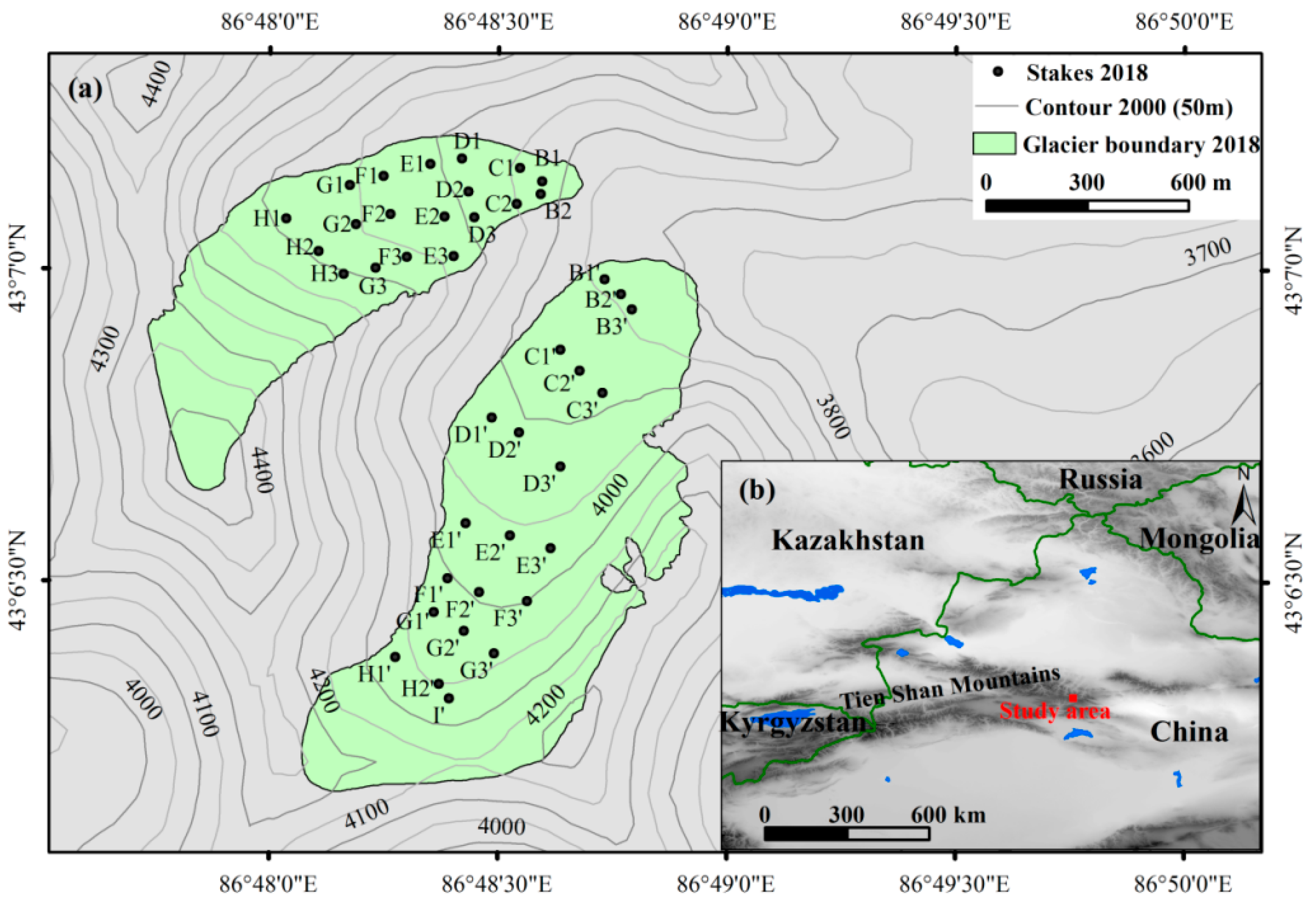
2.1. Study Site

As shown in Figure 1, Urumqi Glacier No. 1 (UG1; 43°06′ N, 86°49′ E) is a northeast-facing valley glacier, located on the northern slope of Tianger Summit II in the eastern Tien Shan, the elevation is between 3752 and 4445 m. In 1959, the Chinese Academy of Sciences established the Tianshan Glaciological Station (TGS) 3 km northeast of the glacier to carry out climatological, glaciological and hydrological observations around this glacier. UG1 separated into two small independent glaciers in 1993, the east branch (UG1E) and west branch (UG1W), due to sustained mass balance losses, with a cumulative mass loss of the glacier of 20 m w.e. from 1980 to 2017 which has driven retreat and area decline. According to the field investigation data, the glacier covered a total area of 1.95 km² in 1962 to 1.54 km² in 2017. The area of UG1E was 0.99 km², which is very close to the average area of glaciers in China (1.01 km²) published in the Second Chinese Glacier Inventory, and slightly larger than the average area of glaciers in China’s Tien Shan Mountains (0.90 km²) [48].

2.2. Materials

2.2.1. Sentinel-1 Ascending and Descending Orbits Data

To generate 3D surface motion displacement of UG1, Sentinel-1 ascending and descending orbit images in the Interfermetric Wide Swath mode were used to test the reliability of the optimized method.

Table A1. Parameter list of Sentinel-1 on Urumqi Glacier No. 1.

Satellite	Track Directions	Track	Acquired Time	Polarization Mode	Incidence Angle/°
Sentinel-1A	Ascending	Track_114	19 April 2018	VV	41.444
			1 May 2018	VV	41.441
			13 May 2018	VV	41.447
			25 May 2018	VV	41.450
			6 June 2018	VV	41.447
			18 June 2018	VV	41.446
			12 July 2018	VV	41.441
			24 July 2018	VV	41.446
			17 August 2018	VV	41.450
			29 August 2018	VV	41.448
Sentinel-1B	Descending	Track_19	19 April 2018	VV	43.851
			1 May 2018	VV	43.843
			13 May 2018	VV	43.845
			25 May 2018	VV	43.848
			6 June 2018	VV	43.853
			18 June 2018	VV	43.850
			12 July 2018	VV	43.847
			24 July 2018	VV	43.846
			17 August 2018	VV	43.849
			29 August 2018	VV	43.850

list the principal parameters for SAR imagery. The pixel spacing in the LOS and azimuth directions were 2.33 and 13.89 m, respectively. In total, 10 ascending and 10 descending SAR images were acquired from 19 April to 29 August 2018. From these, a total of 40 image pairs, which had a time interval for each image pair of less than 36 days, were selected, including 20 ascending pairs and 20 descending pairs (see

Table A2. Sentinel-1 image pairs used on Urumqi Glacier No. 1.

Track Directions	Primary Images	Secondary Images	Baseline (m)	Time Intervals (day)
Ascending	19 April 2018	1 May 2018	45.814	12
	19 April 2018	13 May 2018	−51.462	24
	19 April 2018	25 May 2018	−97.520	36
	1 May 2018	13 May 2018	−93.673	12
	1 May 2018	25 May 2018	−141.855	24
	1 May 2018	6 June 2018	−91.351	36
	13 May 2018	25 May 2018	−48.964	12
	13 May 2018	6 June 2018	18.352	24
	13 May 2018	18 June 2018	31.388	36
	25 May 2018	6 June 2018	52.916	12
	25 May 2018	18 June 2018	76.525	24
	6 June 2018	18 June 2018	25.262	12
	6 June 2018	12 July 2018	100.125	36
	18 June 2018	12 July 2018	74.758	24
	18 June 2018	24 July 2018	3.160	36
	12 July 2018	24 July 2018	−74.824	12
	12 July 2018	17 August 2018	−141.608	36
	24 July 2018	17 August 2018	−67.225	24
	24 July 2018	29 August 2018	−39.664	36
	17 August 2018	29 August 2018	27.249	12
Descending	19 April 2018	1 May 2018	143.474	12
	19 April 2018	13 May 2018	101.273	24
	19 April 2018	25 May 2018	56.725	36
	1 May 2018	13 May 2018	−42.507	12
	1 May 2018	25 May 2018	−88.337	24
	1 May 2018	6 June 2018	−168.091	36
	13 May 2018	25 May 2018	−45.842	12
	13 May 2018	6 June 2018	−125.828	24
	13 May 2018	18 June 2018	−73.370	36
	25 May 2018	6 June 2018	−80.777	12
	25 May 2018	18 June 2018	−29.639	24
	6 June 2018	18 June 2018	52.497	12
	6 June 2018	12 July 2018	101.450	36
	18 June 2018	12 July 2018	49.405	24
	18 June 2018	24 July 2018	59.532	36
	12 July 2018	24 July 2018	18.759	12
	12 July 2018	17 August 2018	−36.185	36
	24 July 2018	17 August 2018	−43.193	24
	24 July 2018	29 August 2018	−72.274	36
	17 August 2018	29 August 2018	−30.089	12

).

2.2.2. Measurement Data

Field measurement of three-dimensional surface motion displacement of glacier is usually made by drilling stakes into the ice and measuring their positions at regular intervals. On 25 April and 29 August 2018, field observations were made on the three-dimensional surface motion displacements of stakes on the east branch and west branch of Urumqi Glacier No.1, respectively, to obtain the three-dimensional surface motion displacement of the glacier during this period. The measurement data were mainly used to evaluate the accuracy of 3D surface displacement of glacier retrieved by the optimized method and Sentinel-1 ascending and descending orbit data. The RTK (Real Time Kinematic Studio) method was used to measure the positions of the stakes. The instrument was Trimble R10 GNSS, and its horizontal and vertical positioning accuracy can reach the order of mm [49]. The number of stakes was 39, of which 21 were placed on the east branch and 18 were placed on the West branch. The position distribution of stakes is shown in Figure 1.

3. Methodology

In previous studies, the methods for inversion of 3D surface motion information of glaciers generally include offset tracking method, estimation of 3D information, and the time series of 3D information. In this paper, the method of optimizing the offset tracking results by means of iterative filtering is added to solve the problems in the actual processing process. The method used in this paper includes four steps: Offset Tracking method, optimizing the offset tracking results by means of iterative filtering, OT-SBAS technology and the conversion of 3D surface motion displacement of the glacier.

3.1. Offset Tracking

Offset tracking (OT) is a technique for measuring surface deformation based on SAR image amplitude information, which can estimate the surface motion displacement in the line of sight (LOS) and azimuth directions. It has been widely used to measure the surface displacement caused by glacier movements, seismic activity and coal mining [50,51,52,53,54,55]. OT includes amplitude tracking and coherence tracking. Amplitude tracking uses amplitude information to correlate two SAR images, which is suitable for situations with clear features and poor coherence of the image pair. Coherence tracking seeks to calculate the interferometric phase information of the SAR image, which requires the image pair to have a certain degree of coherence and is susceptible to temporal decorrelation [19]. This paper used the method of amplitude tracking.

Four main steps were employed to estimate LOS and azimuth offsets using Amplitude Tracking in the trial version SARscape 5.5.2 [56]: (1) precise registration of primary and secondary images, (2) offset calculation based on normalized cross-correlation algorithm, (3) the calculation of system estimation, (4) the calculation of LOS and azimuth displacement. The LOS looks and azimuth Looks were set to 4 and 1 pixels, respectively, for all the SAR image pairs, thereby achieving a ground resolution of approximately 15 m. The size of the small image patch that averaged the cross-correlation function was chosen to be 32 pixels in both and azimuth, we set the cross-correlation coefficient threshold at 0.1, and values below 0.1 were discarded and set to no data.

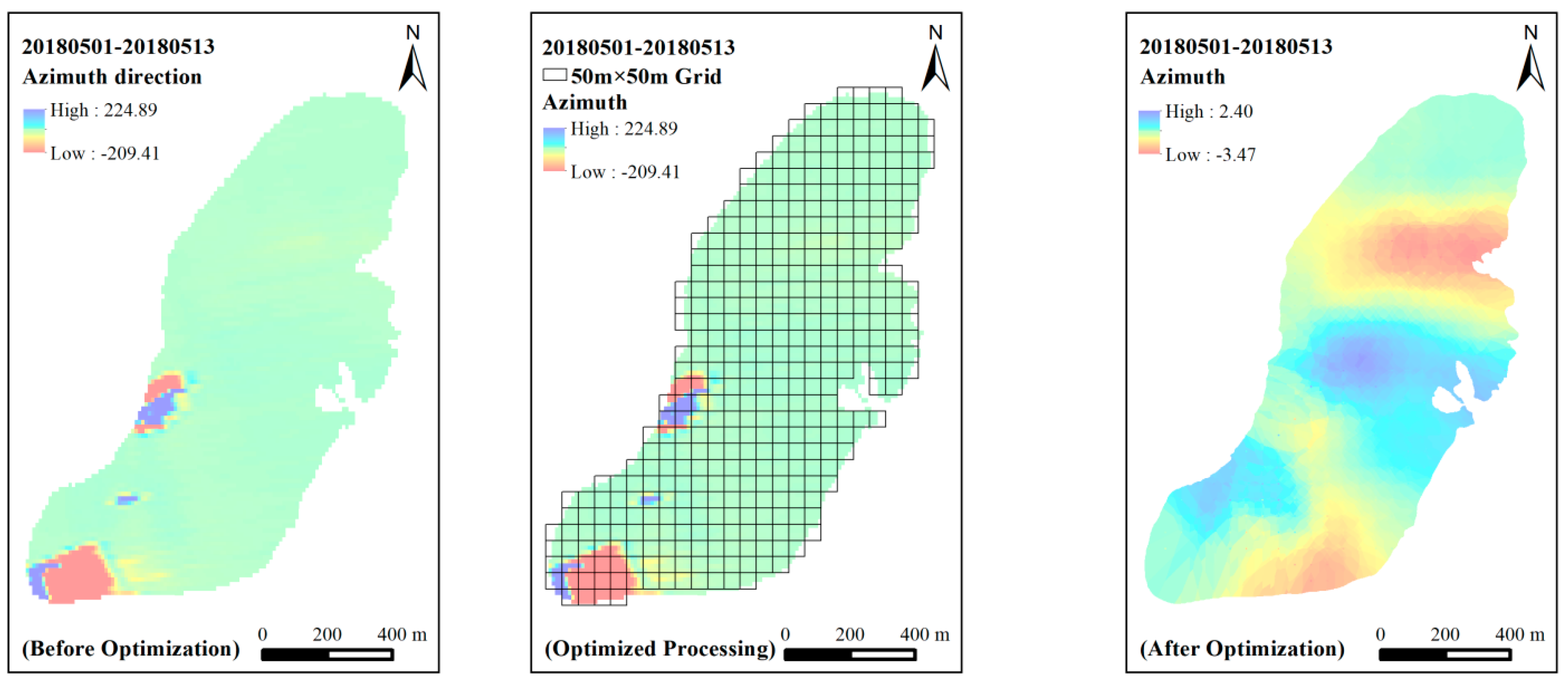
3.2. Optimizing the Offset Tracking Results by Means of Iterative Filtering

According to the field measured values, the processing results of the offset tracking method for each image pair were checked, it was found that the data in some areas was far greater than the field measured value. This was mainly due to the cross-correlation failures of the data, which led to erroneous results in this area, indicating that there were still some shortcomings in the offset tracking method when the software tool used in this study. In order to prevent the transmission of erroneous information to the final result, we needed to optimize the obtained offset tracking results in the line-of-sight and azimuth directions. In this study, we achieved the goal of optimization through an iterative screening process. Figure 2 showed the optimized processing and the results before and after optimization. The specific processing steps were as follows:

(1) A 50 × 50 m grid treatment was carried out on a single glacier, and each grid was checked. When the offset tracking result covered did not exceed 50% of the grid area, the grid was removed. (2) We extracted the average value of offset tracking results covered by each grid after filtering. In order to facilitate subsequent computation, grid data were converted to point data. (3) We obtained the average value $\mathrm{a} ¯$ and standard deviation $\mathsf{\sigma }$ of all points on a single glacier and removed the points whose values were outside the threshold $\overline{\mathrm{a}}\pm 3\mathsf{\sigma }$, then recalculated the average and standard deviation of the remaining point values, and removed the points outside the threshold again, and iterated until all the remaining points fully met the threshold requirements. (4) According to the value of the remaining points after screening, the Ordinary Kriging Interpolation method was used to fill up the value of the missing part, so as to obtain the optimization results of the LOS and azimuth directions of a single glacier.

3.3. OT-SBAS Technology

Offset Tracking-Small Baseline Subset (OT-SBAS) took multiple optimized offset results obtained at different time scales in each direction as the input for SBAS processing, and then obtained the final offset results of time series in each direction by adjusting them [18].

Taking the LOS direction as an example, $N+1$ SAR images are acquired at time $t={\left[t_0,\cdots ,t_N\right]}^T$, and $M$ image pairs can be obtained according to the temporal and spatial baseline threshold:

$$\frac{N+1}{2}\le M\le N\left(\frac{N+1}{2}\right)$$

(1)

Assuming that the acquisition time of the earliest image $t_0$ is the reference time, then the relative offset $\epsilon \left(t_i\right)$ at time $t_i\left(i=1,\cdots ,N\right)$ is the parameter to be solved:

$$\epsilon ={\left[\epsilon \left(t_1\right),\cdots ,\epsilon \left(t_N\right)\right]}^T$$

(2)

Use the offset tracking method to independently calculate the LOS direction offset $\delta {\epsilon }_j\left(j=1,\cdots ,M\right)$ between each offset pair.

$$\delta {\epsilon }_j={\left[\delta {\epsilon }_1,\cdots ,\delta {\epsilon }_M\right]}^T$$

(3)

For $M$ image pairs, the order of acquiring the primary image and the secondary image is $m_j$ and $s_j$ $\left(j=1,\cdots ,M\right)$, respectively, and if the primary and secondary images are arranged in order, thus,

$$\delta {\epsilon }_j=\epsilon \left(t_{m_j}\right)-\epsilon \left(t_{s_j}\right) \left(j=1,\cdots ,M\right)$$

(4)

Equation (4) includes equations with unknown parameters, and it can be rewritten in matrix form as:

$$\delta \epsilon =A\epsilon$$

(5)

where $A=\left[\begin{array}{ccccc}0& -1& 0& +1& \cdots \\ 0& 0& +1& 0& \cdots \\ \cdots & \cdots & \cdots & \cdots & \cdots \\ \cdots & \cdots & \cdots & \cdots & \cdots \end{array}\right]$, each row of matrix $A\left[M\times N\right]$ corresponds to an offset pair.

If all image pairs belong to the same small baseline subset, then the rank of the matrix $A$ is $N\left(M\ge N\right)$, and its least squares solution is provided:

$$\stackrel{\wedge }{\epsilon }=A^{\tau }\delta \epsilon \mathrm{and} A^{\tau }={\left(A^{T}A\right)}^{-1}{A}^T$$

(6)

If the number of the small baseline subset is $L$, the rank of matrix $A$ is $N-L+1$. When $L$ is greater than 1, matrix $A$ is rank defect, and Equation (5) has multiple solutions, so singular value decomposition (SVD) is used to solve the unique value of Equation (5).

$$A=US{W}^T$$

(7)

where $U$ is an orthogonal matrix with dimension $\left[M\times M\right]$; diagonal elements of $S$ are singular values ${\sigma }_i$ $\left(i=1,\cdots ,N\right)$; $W$ is an orthogonal matrix with dimension $\left[N\times N\right]$. The minimum-norm least squares solution of Equation (5) is:

$$\stackrel{\wedge }{\epsilon }=W{S}^{-1}{U}^T\delta \epsilon$$

(8)

In order to obtain a solution that conforms to the physical meaning, the solution of the relative offsets $\epsilon$ was replaced with the solution of the average displacement velocity $\upsilon$:

$$v^T=\left[v_1=\frac{{\epsilon }_1-{\epsilon }_0}{t_1-t_0}, \cdots , v_{\mathit{N}}=\frac{{\epsilon }_{\mathit{N}}-{\epsilon }_{\mathit{N}-1}}{t_{\mathit{N}}-t_{\mathit{N}-1}}\right]$$

(9)

Equation (5) can be transformed into:

$${\displaystyle \sum }_{i=s_j+1}^{m_j}\left(t_i-t_{i-1}\right){\upsilon }_i=\delta {\epsilon }_j \left(j=1,\cdots ,M\right)$$

(10)

Equation (10) can be simplified to:

$$B_1\upsilon =\delta \epsilon$$

(11)

where $B_1$ is a matrix with a dimension of $M\times N$, the matrix element $B_1\left[i,j\right]=\left(t_{j+1}-t_j\right)$ $\left(S_j+1\le j\le m_j,\forall i=1,\cdots ,M\right)$, and all other elements are zero.

$$B_1=\left[\begin{array}{ccccccccc}12& 0& 0& 0& 0& 0& 0& 0& 0\\ 12& 12& 0& 0& 0& 0& 0& 0& 0\\ 12& 12& 12& 0& 0& 0& 0& 0& 0\\ 0& 12& 0& 0& 0& 0& 0& 0& 0\\ 0& 12& 12& 0& 0& 0& 0& 0& 0\\ 0& 12& 12& 12& 0& 0& 0& 0& 0\\ 0& 0& 12& 0& 0& 0& 0& 0& 0\\ 0& 0& 12& 12& 0& 0& 0& 0& 0\\ 0& 0& 12& 12& 12& 0& 0& 0& 0\\ 0& 0& 0& 12& 0& 0& 0& 0& 0\\ 0& 0& 0& 12& 12& 0& 0& 0& 0\\ 0& 0& 0& 0& 12& 0& 0& 0& 0\\ 0& 0& 0& 0& 12& 24& 0& 0& 0\\ 0& 0& 0& 0& 0& 24& 0& 0& 0\\ 0& 0& 0& 0& 0& 24& 12& 0& 0\\ 0& 0& 0& 0& 0& 0& 12& 0& 0\\ 0& 0& 0& 0& 0& 0& 12& 24& 0\\ 0& 0& 0& 0& 0& 0& 0& 24& 0\\ 0& 0& 0& 0& 0& 0& 0& 24& 12\\ 0& 0& 0& 0& 0& 0& 0& 0& 12\end{array}\right]$$

(12)

The optimized offset tracking results provide offsets of 20 periods in each direction ($\delta \epsilon$ in Equation (11)), and the glacier velocities $\upsilon$ for 9 consecutive periods in each direction are estimated by the OT-SBAS method.

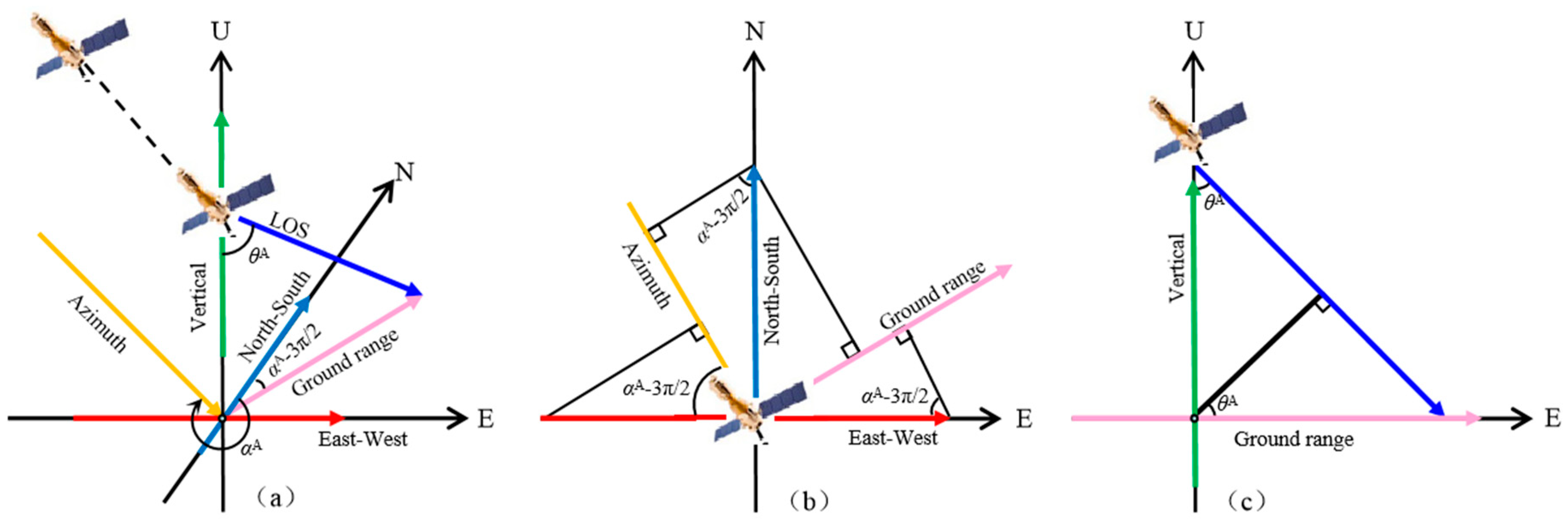
3.4. Conversion of 3D Surface Motion Displacement of Glacier

After OT-SBAS technology processing, glacier velocities in four directions (ascending LOS and azimuth directions and descending LOS and azimuth directions) were obtained, respectively. In order to obtain 3D velocities, we first converted the velocities angle of the above four directions to the east, north and vertical directions, and then calculated them by using the least square method.

Taking the ascending track as an example, as shown in Figure 3, the projection of LOS velocity (${\upsilon }_{LOS}^A$) on the ground is the ground range (GR) velocity (${\upsilon }_{GR}^A$), where the superscript ‘A’ means the ascending track. ${\upsilon }_{GR}^A$ can be regarded as the function of east velocity ${\upsilon }_E^A$ and north velocity ${\upsilon }_N^A$, and ${\upsilon }_{LOS}^A$ is the function of vertical velocity ${\upsilon }_U^A$ and ${\upsilon }_{GR}^A$ [18]:

$${\upsilon }_{GR}^A={\upsilon }_E^A\sin \left({\alpha }^A-3\pi /2\right)+{\upsilon }_N^A\cos \left({\alpha }^A-3\pi /2\right)$$

(13)

$${\upsilon }_{LOS}^A=-{\upsilon }_U^A\cos {\theta }^A+{\upsilon }_{GR}^A\sin {\theta }^A$$

(14)

where ${\alpha }^A$ and ${\theta }^A$ are the radar azimuth and incidence angle, respectively. Based on Equations (13) and (14), the relationship between and 3D velocities can be deduced as follows:

$${\upsilon }_{LOS}^A=-{\upsilon }_U^A\cdot \cos {\theta }^A+{\upsilon }_E^A\sin {\theta }^A\cdot \sin \left({\alpha }^A-\frac{3\pi }{2}\right)+{\upsilon }_N^A\sin {\theta }^A\cdot \cos \left({\alpha }^A-\frac{3\pi }{2}\right)$$

(15)

Meanwhile, the azimuth (AZ) velocity ${\upsilon }_{AZ}^A$ can be expressed a combination of ${\upsilon }_E^A$ and ${\upsilon }_N^A$:

$${\upsilon }_{AZ}^A=-{\upsilon }_E^A\cos \left({\alpha }^A-3\pi /2\right)+{\upsilon }_N^A\sin \left({\alpha }^A-3\pi /2\right)$$

(16)

Similarly, in terms of descending track, we can obtain:

$${\upsilon }_{LOS}^D=-{\upsilon }_U^D\cdot \cos {\theta }^D+{\upsilon }_E^D\sin {\theta }^D\cdot \sin \left({\alpha }^D-3\pi /2\right)+{\upsilon }_N^D\sin {\theta }^D\cdot \cos \left({\alpha }^D-3\pi /2\right)$$

(17)

$${\upsilon }_{AZ}^D=-{\upsilon }_E^D\cos \left({\alpha }^D-3\pi /2\right)+{\upsilon }_N^D\sin \left({\alpha }^D-3\pi /2\right)$$

(18)

where the superscript ‘D’ means descending track.

Therefore, the 3D velocity can be retrieved using the LOS and azimuth direction velocities derived from ascending and descending images. It can be expressed as a simplified matrix, as shown below:

$$B_{2}X=L$$

(19)

where

$$B_2=\left[\begin{array}{ccc}-\cos {\theta }^A& \sin {\theta }^A\cdot \sin \left({\alpha }^A-3\pi /2\right)& \sin {\theta }^A\cdot \cos \left({\alpha }^A-3\pi /2\right)\\ 0& -\cos \left({\alpha }^A-3\pi /2\right)& \sin \left({\alpha }^A-3\pi /2\right)\\ -\cos {\theta }^D& \sin {\theta }^D\cdot \sin \left({\alpha }^D-3\pi /2\right)& \sin {\theta }^D\cdot \cos \left({\alpha }^D-3\pi /2\right)\\ 0& -\cos \left({\alpha }^D-3\pi /2\right)& \sin \left({\alpha }^D-3\pi /2\right)\end{array}\right]$$

(20)

$$X={\left[\begin{array}{ccc}{\upsilon }_U& {\upsilon }_E& {\upsilon }_N\end{array}\right]}^T$$

(21)

$$L={\left[\begin{array}{cccc}{\upsilon }_{LOS}^A& {\upsilon }_{AZ}^A& {\upsilon }_{LOS}^D& {\upsilon }_{AZ}^D\end{array}\right]}^T$$

(22)

Since errors are inevitable in the calculation process, taking error factors into account, Equation (19) should be expressed as:

$$B_{2}X+V=L$$

(23)

where $V$ is the errors vector. We use a least squares procedure to acquire the optimal estimation of 3D velocities, as follows:

$$\stackrel{\wedge }{X}={\left(B_2^{T}P{B}_2\right)}^{-1}{B}_2^{T}PL$$

(24)

$${\delta }_{\stackrel{\wedge }{X}}^2={\left(B_2^{T}P{B}_2\right)}^{-1}$$

(25)

where ${\delta }_{\stackrel{\wedge }{X}}^2$ is the variance of $\stackrel{\wedge }{X}$, $P$ is the matrix of the weight. Assuming that the velocity observations in the four directions are independent, we can get [18]:

$$P=\left[\begin{array}{cccc}{\left({\delta }_{LOS}^A\right)}^2& 0& 0& 0\\ 0& {\left({\delta }_{AZ}^A\right)}^2& 0& 0\\ 0& 0& {\left({\delta }_{LOS}^D\right)}^2& 0\\ 0& 0& 0& {\left({\delta }_{AZ}^D\right)}^2\end{array}\right]$$

(26)

where ${\delta }_{LOS}^A$, ${\delta }_{AZ}^A$, ${\delta }_{LOS}^D$ and ${\delta }_{AZ}^D$ are the standard deviations of ${\upsilon }_{LOS}^A$, ${\upsilon }_{AZ}^A$, ${\upsilon }_{LOS}^D$ and ${\upsilon }_{AZ}^D$. If the center point $\left(x,y\right)$ of velocity observation in the regular window obey a Gaussian distribution, then the standard deviation $\delta$ of velocity observation at point $\left(x,y\right)$ can be calculated as follow [18,57]:

$$\delta =\sqrt{\frac{{{\displaystyle \sum }}_n{\left(\upsilon \left(I,J\right)-\overline{\upsilon }\left(I,J\right)\right)}^2}{n-1}}$$

(27)

where $\upsilon \left(I,J\right)$ are the observations, $\overline{\upsilon }\left(I,J\right)$ are the averages of observations within the regular window, $n$ is the number of observations in the window.

The initial weight matrix $P$ is determined by the standard deviation of the velocity observations $\delta$. The calculation of the 3D velocity $\stackrel{\wedge }{X}$ needs to be iterated. In the iterative process, the iteration method with variable weights of robust estimation is used to adjust $P$ according to the corresponding elements of $V$ [18,58]. The IGGIII method is used as the weight function in this paper.

$$P\left(V\right)=\{\begin{array}{l}P\left(V\right),\\ \frac{1.5\sigma }{\left|V\right|}P\left(V\right),\\ 0,\end{array}\begin{array}{c}\end{array}\begin{array}{l}\left|V\right|\le 1.5\sigma \\ 1.5\sigma <\left|V\right|<2.5\sigma \\ \left|V\right|\le 2.5\sigma \end{array}$$

(28)

where $\sigma$ is the error in the prior unit weight, and $\left|V\right|$ is the absolute value of the residual.

According to the actual measurement data obtained, we ensured that the iteration proceeded until improvement was less than 0.01 cm/day, and the 3D surface motion velocities of glacier in the final time series were obtained. Finally, according to the time interval of each period and the 3D surface motion velocity of glacier, the 3D surface motion displacement of glacier during the whole study period was obtained.

In this study, Sentinel-1A and Sentinel-1B data incident angles ${\theta }^A$ and ${\theta }^D$ are shown in Table A1 of Appendix A. The azimuth angles ${\alpha }^A$ and ${\alpha }^D$ of Sentinel-1A and Sentinel-1B data are −13.787° and −166.166°, respectively. Therefore, Equation (20) can be obtained:

$$B_2=\left[\begin{array}{ccc}-0.750& 0.643& 0.158\\ 0& -0.238& 0.971\\ -0.721& -0.673& 0.166\\ 0& -0.239& -0.971\end{array}\right]$$

(29)

4. Results and Discussion

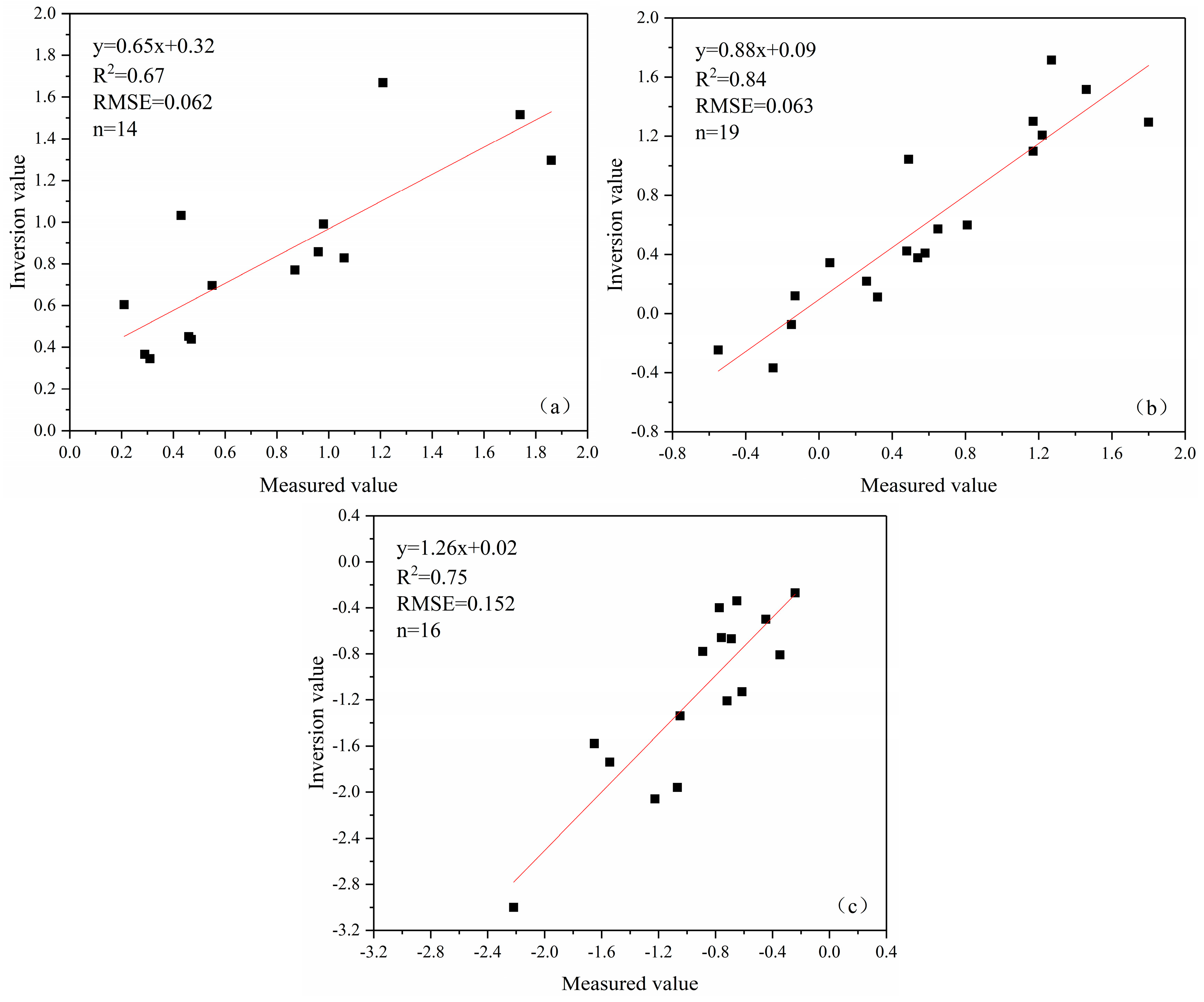
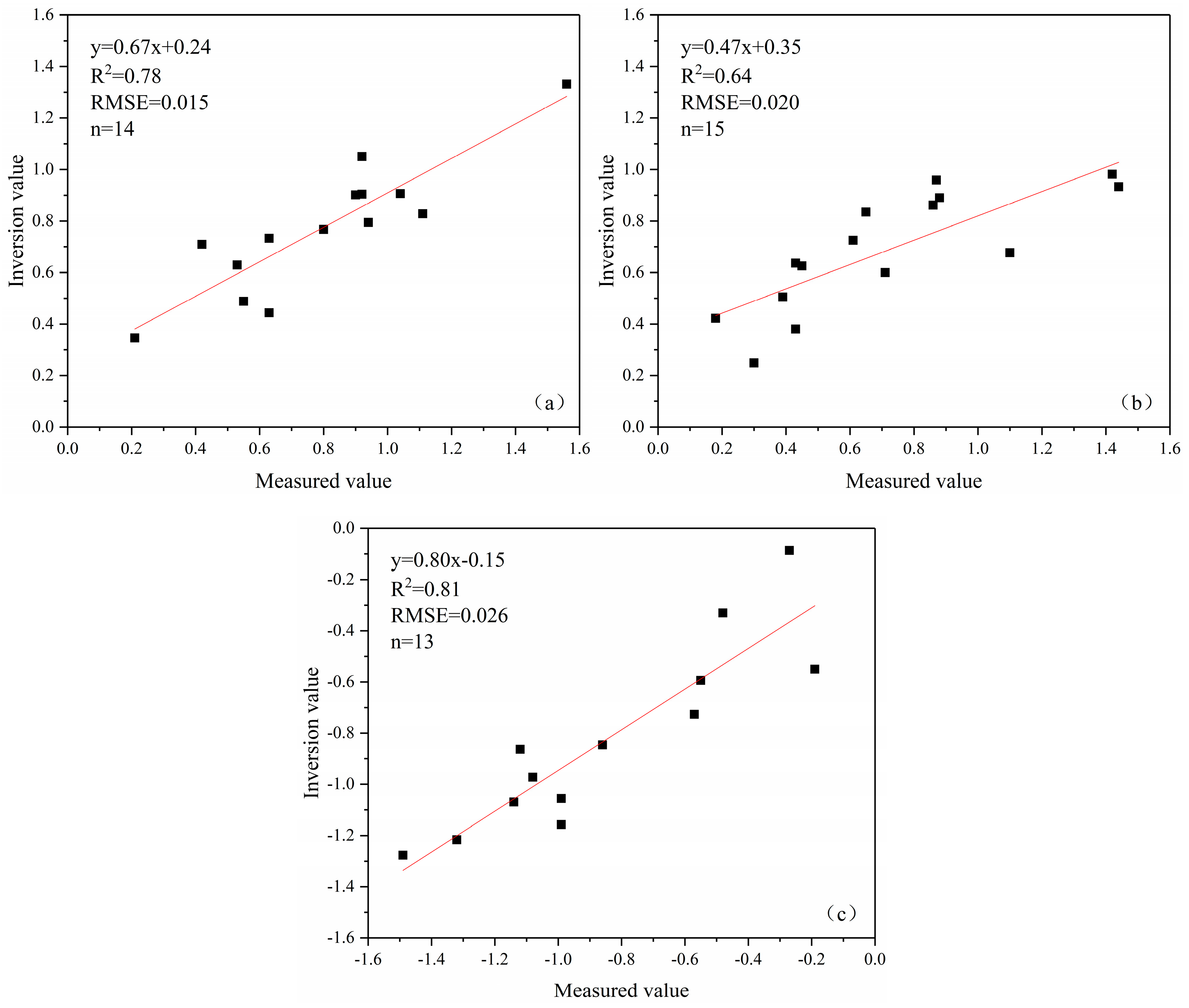
4.1. Comparison between the Inversion Value and the Measured Value

When verifying the reliability of the glacier movement monitoring results, the time period of the remote sensing images of UG1 was obtained from 19 April to 29 August 2018, and the situ measurement period in the field was 25 April 2018 and 29 August 2018. Therefore, before comparing the measured three-dimensional surface motion displacement of the glacier with the inversion results, in order to ensure that the inversion period corresponds to the situ measurement period, the 3D surface motion displacement of the glacier for the time interval is calculated by the average velocity in the first period, obtained through inversion, and the time interval between the actual measurement start time and the end time of the first inversion period.

Since the in situ measurement data are related to displacement, when comparing the measured value of UG1 with the remote sensing inversion result, it needs to be converted into the displacement in each period according to the average velocity obtained from the inversion and time interval. The displacement $S_D$ of UG1 in the east, north and vertical directions can be obtained from the glacier surface velocity ${\upsilon }_i(i=1,\cdots ,9)$ in each direction in nine periods and the time interval $T_i(i=1,\cdots ,9)$ in each period. Its calculation equation is as follows:

$$S_D={\displaystyle \sum }_{i=1}^9\left({\upsilon }_i\times T_i\right)$$

(30)

where $D$ is east, north and vertical direction.

When inverting the motion velocity of glacier, in order to prevent the pixel position from shifting during processing, set a 20 m buffer zone with each stake as the center, and then calculate the average value of the pixels in the buffer zone and use it as the inversion result of the position of stake.

The remote sensing inversion values of 3D surface movement displacements of UG1E and UG1W were compared with the actual measured values, as shown in Figure 4 and Figure 5,

Table 1. The inversion value and the measured value of UG1E in three directions (unit: m).

Stakes	East		North		Vertical
	Inversion Value	Measured Value	Inversion Value	Measured Value	Inversion Value	Measured Value
B1′	0.83	1.06	0.60	0.81	−1.07	−1.96
B2′	0.86	0.96	0.57	0.65	−1.23	−2.06
B3′	0.89	1.73	0.69	0.05	−2.22	−3.00
C1′	1.03	0.43	0.11	0.32	−1.54	−1.74
C2′	1.30	1.86	0.41	0.58	−1.65	−1.58
C3′	1.67	1.21	0.38	0.54	−0.72	−1.21
D1′	1.16	−0.71	−0.08	−0.15	−1.05	−1.34
D2′	1.52	1.74	0.42	0.48	−0.61	−1.13
D3′	2.07	0.07	1.10	1.17	−2.19	−1.34
E1′	0.37	0.29	0.34	0.06	0.12	−0.80
E2′	0.34	0.31	1.52	1.46	−0.35	−0.81
E3′	0.99	0.98	1.30	1.17	−1.25	−0.48
F1′	0.38	−0.31	0.12	−0.13	−0.45	−0.50
F2′	0.60	0.21	1.29	1.80	−0.89	−0.78
F3′	0.70	0.55	1.72	1.27	−0.76	−0.66
G1′	0.96	−0.24	0.25	−0.55	−0.77	−0.40
G2′	0.53	0.09	0.43	0.80	−1.22	−0.44
G3′	0.45	0.46	1.21	1.22	−1.60	−0.76
H1′	1.46	−0.97	−0.37	−0.25	−0.69	−0.67
H2′	0.77	0.87	0.22	0.26	−0.24	−0.27
I′	0.44	0.47	1.04	0.49	0.65	−0.34

and

Table 2. The inversion value and the measured value of UG1W in three directions (unit: m).

Stakes	East		North		Vertical
	Inversion Value	Measured Value	Inversion Value	Measured Value	Inversion Value	Measured Value
B1	0.43	−0.10	0.94	−0.80	−0.51	−1.69
B2	0.30	0.92	0.73	0.61	−1.18	−1.89
C1	0.73	0.63	0.93	1.44	−0.73	−0.57
C2	0.79	0.94	0.84	0.65	−1.12	−1.87
D1	0.35	0.21	0.51	0.39	−1.07	−1.14
D2	0.90	0.90	0.60	0.71	−0.32	−1.40
D3	0.80	0.39	0.68	1.10	−1.28	−1.49
E1	0.63	0.53	0.38	0.43	−1.22	−1.32
E2	0.83	1.11	0.94	0.57	−0.24	−1.10
E3	0.49	0.55	0.42	0.18	−1.06	−0.99
F1	0.44	0.63	0.70	−0.67	−1.16	−0.99
F2	0.77	0.80	0.98	1.42	−0.97	−1.08
F3	0.55	0.17	0.96	0.87	−0.85	−0.86
G1	0.71	0.42	0.25	0.30	−0.59	−0.55
G3	0.91	1.04	0.63	0.45	−0.33	−0.48
H1	1.05	0.92	0.64	0.43	−0.09	−0.27
H2	1.33	1.56	0.89	0.88	−0.86	−1.12
H3	0.90	0.92	0.86	0.86	−0.55	−0.19

, respectively. In the figure, regarding the two figures marked at each stake, the upper one is the remote sensing inversion value, while the lower one is the in situ measurement value. Positive or negative numbers indicate the direction of movement. Velocities in the east, north, and upward directions are positive numbers.

The inverted values of the glacier motion velocity at the stakes were roughly the same as the measurement values, but the inverted values of very few stakes were quite different from the value measured, due to the measured displacement of stake being a point measurement, While the motion velocity obtained by the inversion was the average value of the pixel. In addition, there was a certain degree of contingency in the placement of stakes, so the values measured by individual stakes might have randomness, which could not accurately represent the value of the corresponding pixels, resulting in a large difference between the inversion value and the value measured. However, if there was a good correspondence between the inversion values of most of the stakes and the values measured, it could also prove the feasibility of the optimized inversion method for the 3D surface motion and displacement of the glacier.

Therefore, when evaluating the accuracy of the inversion values of the glacier 3D surface motion velocity at the stakes, the accuracy of the inversion results was evaluated by using the majority values of the remaining stakes after removing the few stakes that differ greatly from the measured values.

4.2. Accuracy Evaluation of Inversion Results

As is shown in Figure 6, the correlation coefficients between the inverted displacement values and the measured displacement values of UG1E in the east, north, and vertical directions were 0.67, 0.84, and 0.75, respectively, and the root mean square error was 0.062, 0.063, and 0.152 m, respectively. According to the calculation, in the east direction, the average absolute value of the measured value was 0.814, while the average absolute value of the difference between the measured value and the inversion value was 0.213, and the latter accounted for 26.2% of the former. In the north direction, the average absolute value of the measured value was 0.703, while the average absolute value of the difference between the measured value and the inversion value was 0.197, which accounted for 27.9% of the former.

Figure 7 is similar to Figure 6. The correlation coefficients between the inverted displacement value and the measured displacement value of UG1W in the east, north and vertical directions were 0.78, 0.64, and 0.81, respectively, and the root mean square error were 0.015, 0.020, and 0.026 m, respectively. The calculation showed that, in the east direction, the average of the absolute value of the measured value was 0.797, and the average absolute value of the difference between the measured value and the inversion value was 0.132, with the latter accounting for 16.5% of the former. In the north direction, the average absolute value of the measured value was 0.714, and the average of the absolute value of the difference from the inversion value was 0.181, the latter accounting for 25.3% of the former. In the vertical direction, the average absolute value of the measured value was 0.850, while the average absolute value of the difference between the measured value and the inversion value was 0.145, with the latter accounting for 17.1% of the former.

In summary, the accuracy of the inversion results was similar in the east and north horizontal directions of the UG1E, while the accuracy of the inversion results in the vertical direction was lower than that in the horizontal direction. In the UG1W, the accuracy of the inversion results was similar in the east and vertical directions, while in the north direction, the accuracy of the inversion results was lower than that in the east and vertical directions.

Li et al. used the method including SAR offset-tracking, pixel offset-small baseline subset processing and resolution of 3D velocities to obtain the velocity of the Southern Inylchek Glacier in the east, north and vertical directions. The velocities of the glacier were 58 cm/day east, 70 cm/day north, and 113 cm/day vertically, and the errors ranged from 1.1 to 2.2 cm/ day for east velocity, from 0.7 to 1.5 cm/day for north velocity, and from 0.6 to 1.2 cm/day for vertical velocity. Therefore, in the east, north and vertical directions, the percentage of the velocity error in the glacier motion velocity is 1.9–3.8%, 1–2.14% and 0.53–1.06%, respectively.

Yang et al. used methods including offset tracking method, estimation of 3D displacement, and the time series of 3D displacement to retrieve the horizontal and vertical motion velocities of Cuolangma glaciers from January to December 2018. It could be concluded that the velocity error of Cuolangma glacier No.1 in vertical direction accounts for 12.35% of the velocity, and the value for Cuolangma glacier No.2 was 13.5%.

In this study, in the east, north and vertical directions, the percent ranges of the inversion accuracy and the average of the stake measurement values on the UG1E were 7.61%, 8.94% and 13.18%, respectively, and the percent ranges of the inversion accuracy and the average of the stake measurement values on the UG1W were 1.88%, 2.80% and 2.87%, respectively.

It could be seen from the above that the accuracy of the inversion results of this study was similar to that of previous studies. It showed that the optimized method in this paper had good applicability for retrieving the three-dimensional surface motion displacement of high-latitude mountain glaciers in China.

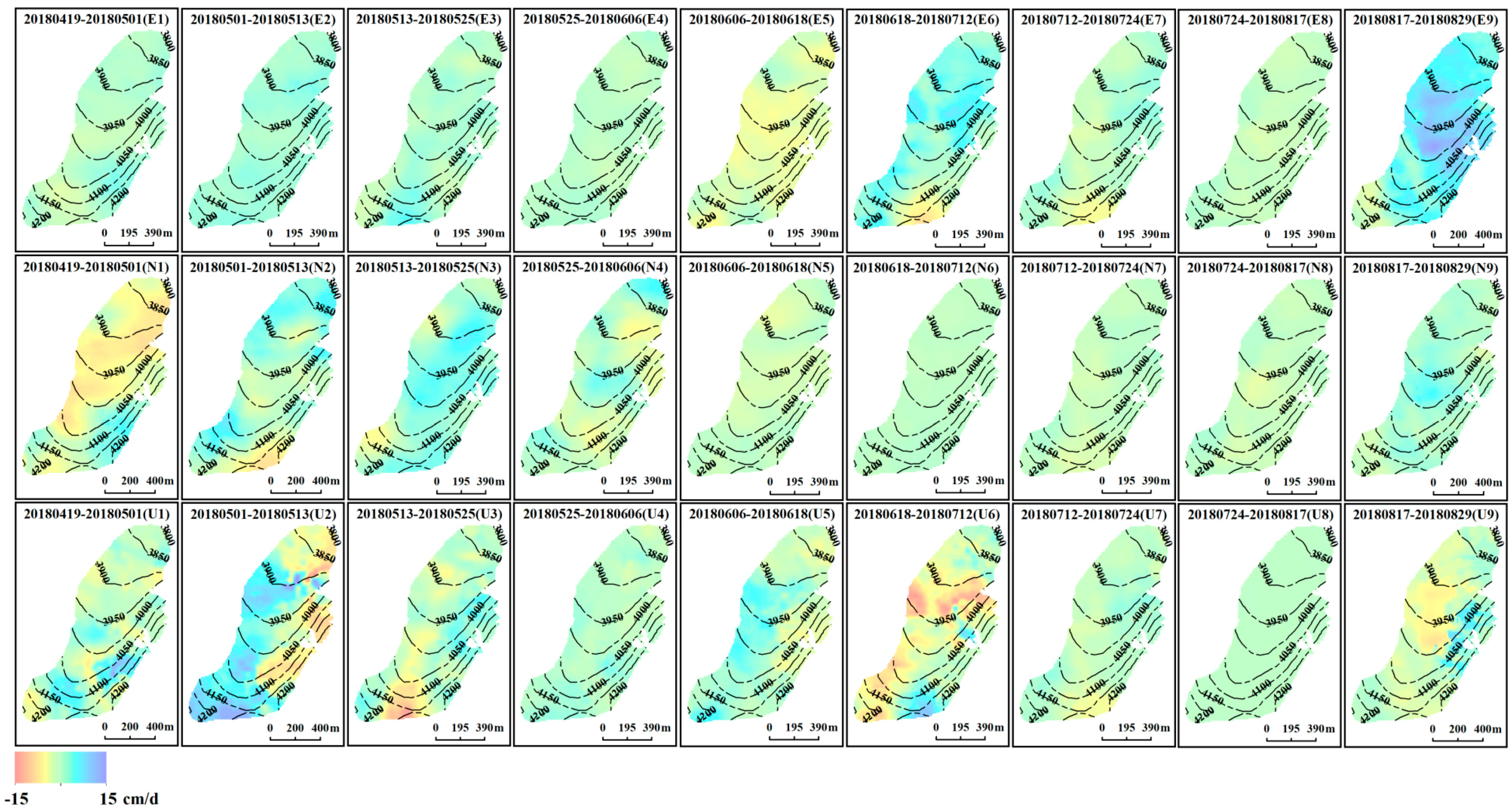
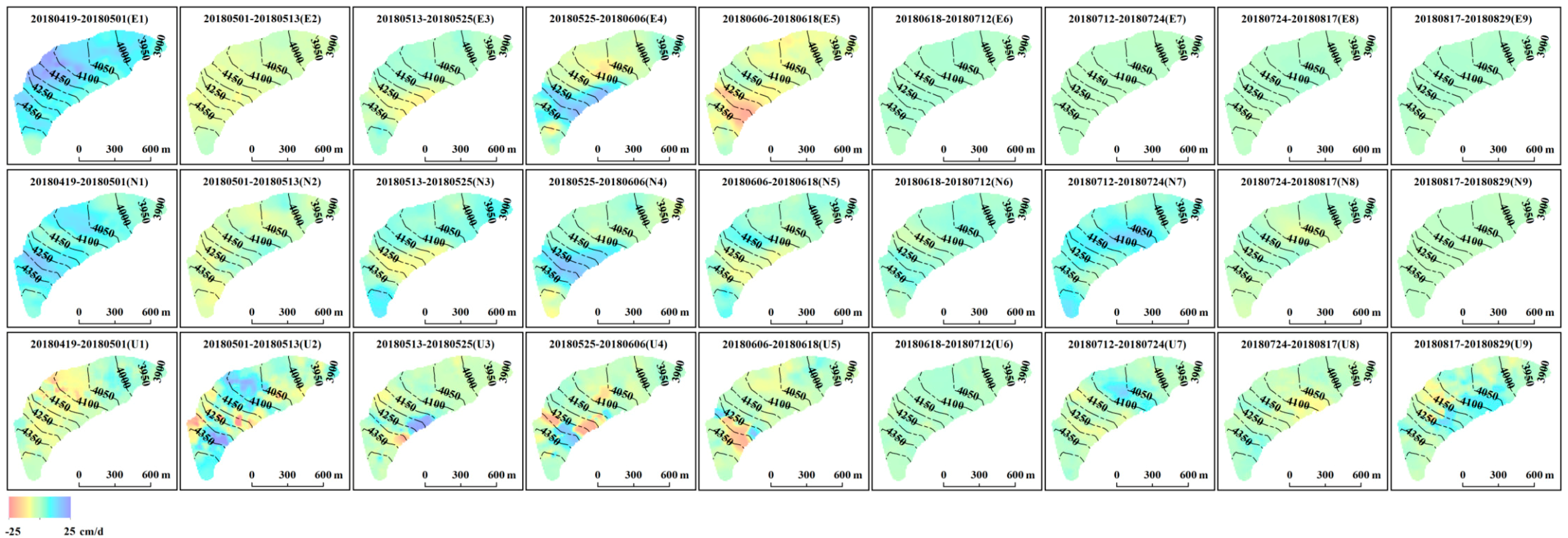
4.3. Distribution of the 3D Surface Motion Velocity of UG1

The distribution of surface motion velocity in the east, north and vertical directions on the east branch and west branch of UG1 are shown in Figure 8 and Figure 9. The distribution characteristics of the surface motion velocity of the east branch and west branch of UG1 glacier are different in the three directions, but generally present a trend of higher values in the middle and lower values on both sides in the same altitude zone.

Figure 8 shows that the surface motion velocity of UG1E distributes smoothly in the east and north directions, and the distribution is relatively discrete in the vertical direction. The east velocity generally shows a movement from west to east, and the speed gradually increases with the passage of time. In the north direction, the velocity in the middle and end of the glacier is higher, which is related to the melting of the glacier. In the vertical direction, the change in the velocity is more complicated, which is mainly caused by the movement of the glacier along the slope, the subsidence or uplift of some areas caused by external forces, and the thinning of the glacier thickness caused by the accelerated melting of the glacier.

It can be seen from Figure 9 that the changes in the surface motion velocity of the western branch glacier in the east and north directions are mainly concentrated in the period of 19 April to 18 June 2018 from the perspective of time. From the spatial point of view, the changes are mainly distributed in the upper and middle reaches of the glacier, which are mainly affected by the mass transfer of the glacier. In the vertical direction, the spatial distribution of the surface motion velocity of UG1W is relatively discrete and complex, and the time change has no obvious change characteristics, which is consistent with the fact that the surface motion velocity of UG1E changes in the vertical direction.

5. Conclusions and Outlook

This paper has presented an optimized method for retrieving the 3D surface motion displacement of glaciers from Sentinel-1 ascending and descending datasets. The optimized method consists of the Offset Tracking method, optimizing the offset tracking results by means of iterative filtering, OT-SBAS technology and conversion of 3D surface motion displacement of glacier. The 3D surface motion displacement of the UG1E and UG1W from 19 April to 29 August 2018 was calculated using Sentinel-1 datasets and the optimized method, respectively, and the accuracy of the retrieval results was evaluated using the in situ measurements.

The comparison between the in situ measurements and the estimated 3D surface motion displacements showed that the accuracies of the inverted displacements of east branch of Urumqi Glacier No. 1 were about 0.062, 0.063, and 0.152 m in the east, north and vertical directions, and these values for the west branch of Urumqi Glacier No. 1 were 0.015, 0.020, and 0.026 m, respectively. The accuracy level should satisfy the general requirement of the 3D surface motion displacement monitoring of high-latitude mountain glaciers in China.

In this study, it has been demonstrated that the optimized monitoring method of 3D surface motion displacement based on the Sentinel-1 ascending and descending orbit data has great potential in glaciology. However, in order to obtain more high-precision 3D glacier surface motion information, the research method in this paper should be further optimized and enhancing the ability of offset tracking method to identify feature points. In addition, since this paper mainly studies the optimization of the method, the research period is short, and it is difficult to determine the relationship with its influencing factors, such as temperature and precipitation. We will discuss the relationship between the 3D surface motion displacement of glacier and its influencing factors in our future research.

References

1. Shi, Y.F.; Huang, M.H.; Yao, T.D.; Deng, Y.X. Glaciers and Their Environments in China: The Present, Past and Future; Science Press: Beijing, China, 2000; ISBN 7030081269. [Google Scholar]
2. Thiel, K.; Arndt, A.; Wang, P.; Li, H.; Li, Z.; Schneider, C. Modeling of Mass Balance Variability and Its Impact on Water Discharge from the Urumqi Glacier No. 1 Catchment, Tian Shan, China. Water 2020, 12, 3297. [Google Scholar] [CrossRef]
3. Benn, D.I.; Warren, C.R.; Mottra, R.H. Calving processes and the dynamics of calving glaciers. Earth-Sci. Rev. 2007, 82, 144–179. [Google Scholar] [CrossRef]
4. Paul, F.; Bolch, T.; Kääb, A.; Nagler, T. The glaciers climate change initiative: Methods for creating glacier area, elevation change and velocity products. Remote Sens. Environ. 2015, 162, 408–426. [Google Scholar] [CrossRef] [Green Version]
5. Guan, W.J.; Cao, B.; Pan, B.T. Research of glacier flow velocity: Current situation and prospects. J. Glaciol. Geocryol. 2020, 42, 1101–1114. (In Chinese) [Google Scholar]
6. Xu, S.Q.; E, D.C.; Wang, S.D. Glacier movement monitoring on Nelson Ice Cap, Antarctica. J. Geomatics 1988, 4, 30–35. (In Chinese) [Google Scholar]
7. Jing, Z.F.; Zhou, Z.M.; Liu, L. Progress of the Research on Glacier Velocities in China. J. Glaciol. Geocryol. 2010, 32, 749–754. (In Chinese) [Google Scholar]
8. Dehecq, A.; Gourmelen, N.; Gardner, A.S.; Brun, F.; Goldberg, D.; Nienow, P.W.; Berthier, E.; Vincent, C.; Wagnon, P.; Trouvé, E. Twenty-first century glacier slowdown driven by mass loss in High Mountain Asia. Nat. Geosci. 2019, 13, 2189–2202. [Google Scholar] [CrossRef]
9. Rydt, J.D.; Reese, R.; Fernando, P.; Gudmundsson, G.H. Drivers of Pine Island Glacier speed-up between 1996 and 2016. Cryosphere 2021, 15, 113–132. [Google Scholar] [CrossRef]
10. Lei, Y.B.; Yao, T.D.; Tian, L.D.; Sheng, Y.W.; Zhu, L.; Liao, J.J.; Zhao, H.B.; Yang, W.; Yang, K.; Berthier, E.; et al. Response of downstream lakes to Aru glacier collapses on the western Tibetan Plateau. Cryosphere 2020, 15, 199–214. [Google Scholar] [CrossRef]
11. Mohr, J.J.; Reeh, N.; Madsen, S.N. Three-dimensional glacial flow and surface elevation measured with radar interferometry. Nature 1998, 391, 273–276. [Google Scholar] [CrossRef]
12. Gudmundsson, S.; Gudmundsson, M.T.; Björnsson, H.; Sigmundsson, F.; Rott, H.; Carstensen, J.M. Three-dimensional glacier surface motion maps at the Gja’lp eruption site, Iceland, inferred from combining InSAR and other ice-displacement data. Ann. Glaciol. 2002, 34, 315–322. [Google Scholar] [CrossRef] [Green Version]
13. Mohr, J.J.; Reeh, N.; Madsen, S.N. Accuracy of three-dimensional glacier surface velocities derived from radar interferometry and ice-sounding radar measurements. J. Glaciol. 2003, 49, 210–222. [Google Scholar] [CrossRef]
14. Magnússon, E.; Rott, H.; Björnsson, H.; Roberts, M.J. Unsteady Glacier Flow Revealed by Multi-Source Satellite Data. In Proceedings of the Agu Fall Meeting, San Francisco, CA, USA, 1–15 December 2006. [Google Scholar]
15. Gray, L. Using multiple RADARSAT InSAR pairs to estimate a full three-dimensional solution for glacial ice movement. Geophys. Res. Lett. 2011, 38, L05502. [Google Scholar] [CrossRef]
16. Hu, J.; Li, Z.W.; Li, J.; Zhang, L.; Ding, X.L.; Zhu, J.J.; Sun, Q. 3-D movement mapping of the alpine glacier in Qinghai-Tibetan Plateau by integrating D-InSAR, MAI and Offset-Tracking: Case study of the Dongkemadi Glacier. Glob. Planet. Chang. 2014, 118, 62–68. [Google Scholar] [CrossRef]
17. Reeh, N.; Madsen, S.N.; Mohr, J.J. Combining SAR interferometry and the equation of continuity to estimate the three-dimensional glacier surface-velocity vector. J. Glaciol. 1999, 45, 533–538. [Google Scholar] [CrossRef] [Green Version]
18. Li, J.; Li, Z.W.; Wu, L.X.; Xu, B.; Hu, J.; Zhou, Y.S.; Miao, Z.L. Deriving a time series of 3D glacier motion to investigate interactions of a large mountain glacial system with its glacial lake: Use of Synthetic Aperture Radar Pixel Offset-Small Baseline Subset technique. J. Hydrol. 2018, 559, 596–608. [Google Scholar] [CrossRef]
19. Yang, L.Y.; Zhao, C.Y.; Zhong, L.; Yang, C.S.; Zhang, Q. Three-Dimensional Time Series Movement of the Cuolangma Glaciers, Southern Tibet with Sentinel-1 Imagery. Remote Sens. 2020, 12, 3466. [Google Scholar] [CrossRef]
20. Bolch, T. Climate change and glacier retreat in northern Tien Shan(Kazakhstan/Kyrgyzstan) using remote sensing data. Glob. Planet. Chang. 2007, 56, 1–12. [Google Scholar] [CrossRef]
21. Shen, Y.P.; Wang, G.Y.; Ding, Y.J.; Mao, W.Y.; Liu, S.Y.; Wang, S.D.; Mamatkanov, D.M. Changes in Glacier Mass Balance in Watershed of Sary Jaz-Kumarik Rivers of Tianshan Mountains in 1957–2006 and Their Impact on Water Resources and Trend to End of the 21th Century. J. Glaciol. Geocryol. 2009, 31, 792–800. (In Chinese) [Google Scholar]
22. Kääb, A.; Berthier, E.; Nuth, C.; Gardelle, J. Contrasting patterns of early twenty-first-century glacier mass change in the Himalayas. Nature 2012, 488, 495–498. [Google Scholar] [CrossRef] [PubMed]
23. Gardelle, J.; Berthier, E.; Amaud, Y. Slight mass gain of Karakoram glaciers in the early twenty-first century. Nat. Geosci. 2012, 5, 322–325. [Google Scholar] [CrossRef]
24. Immerzeel, W.W.; Kraaijenbrink, P.; Shea, J.M.; Shrestha, A.B. High-resolution monitoring of Himalayan glacier dynamics using unmanned aerial vehicles. Remote Sens. Environ. 2014, 150, 93–103. [Google Scholar] [CrossRef]
25. Jiang, Z.L.; Wang, L.; Zhang, Z.; Liu, S.Y.; Zhang, Y.; Tang, Z.G.; Wei, J.F.; Huang, D.N.; Zhang, S.S. Surface elecation changes of Yengisogat Glacier between 2000 and 2014. Arid Land Geograph. 2020, 43, 12–19. (In Chinese) [Google Scholar]
26. LI, Z.J.; Wang, N.L.; Chen, A.A.; Liu, K. Remote sensing monitoring of glacier changes in Shyok basin of the Karakoram Mountains, 1993–2016. J.Glaciol. Geocryol. 2019, 41, 770–782. (In Chinese) [Google Scholar]
27. Xu, A.W.; Yang, T.B.; Wang, C.Q.; Ji, Q. Variation of glaciers in the Shaksgam River Basin, Karakoram Mountains during 1978–2015. Prog. Geograph. 2016, 35, 878–888. (In Chinese) [Google Scholar]
28. Yao, T.D.; Thompson, L.; Yang, W. Different glacier status with atmospheric circulations in Tibetan Plateau and surroundings. Nat. Clim. Chang. 2012, 2, 663–667. [Google Scholar] [CrossRef]
29. Fujita, K.; Ageta, Y. Effect of summer accumulation on glacier mass balance on the Tibetan Plateau revealed by mass-balance model. J. Glaciol. 2000, 46, 244–252. [Google Scholar] [CrossRef] [Green Version]
30. Zhao, Q.D.; Ding, Y.J.; Wang, J.; Gao, H.K. Projecting climate change impacts on hydrological processes on the Tibetan Plateau with model calibration against the glacier inventory data and observed streamflow. J. Hydrol. 2019, 573, 60–81. [Google Scholar] [CrossRef]
31. Wang, X.N.; Yang, T.B.; Tian, H.Z.; Jiang, S. Response of glacier variation in the southern Altai Mountains to climate change during the last 40 years. J. Arid Land Res. Environ. 2013, 27, 77–82. (In Chinese) [Google Scholar]
32. Wang, P.Y.; Li, Z.Q.; Li, H.L.; Wang, W.B. Characteristics of a partially debris-covered glacier and its response to atmospheric warming in Mt. Tomor, Tien Shan, China. Glob. Planet. Chang. 2017, 159, 11–24. [Google Scholar] [CrossRef]
33. Xu, C.H.; Li, Z.Q.; Li, H.L.; Wang, F.T.; Zhou, P. Long-range terrestrial laser scanning measurements of annual and intra-annual mass balances for Urumqi glacier No. 1, eastern Tien Shan, China. Cryosphere 2019, 13, 2361–2383. [Google Scholar] [CrossRef] [Green Version]
34. Yao, X.J.; Liu, S.Y.; Guo, W.Q.; Huai, B.J.; Sun, M.P.; Xu, J.L. Glacier change of Altay Mountain in China from 1960 to 2009-Based on the Second Glacier Inventory of China. J. Nat. Resour. 2012, 27, 1734–1745. (In Chinese) [Google Scholar]
35. Wang, Y.Q.; Zhao, J.; Li, Z.Q.; Zhang, M.J. Glacier changes in the Sawuer Mountain during 1977-2017 and their response to climate change. J. Nat. Resour. 2019, 34, 802–814. (In Chinese) [Google Scholar]
36. Jin, H.A.; Yao, X.J.; Zhang, D.H. A dataset of glacier length in Chinese Altay Mountains from 1959 to 2016. Sci. Data Bank 2019, 4, 168–175. (In Chinese) [Google Scholar]
37. Huai, B.J.; Li, Z.Q.; Wang, F.T.; Wang, P.Y.; Li, K.M. Ice thickness distribution and ice volume estimation of Muz Taw Glacier in Sawir Mountains. Earth Sci. 2016, 41, 757–764. (In Chinese) [Google Scholar]
38. Li, Z.Q.; Shen, Y.P.; Wang, F.T.; Li, H.L.; Dong, Z.W.; Wang, W.B.; Wang, L. Response of Glacier Melting to Climate Change-Take Urumqi Glacier No. 1 as an Example. J. Glaciol. Geocryol. 2007, 29, 333–342. (In Chinese) [Google Scholar]
39. Li, Z.Q.; Shen, Y.P.; Wang, F.T.; Li, H.L.; Dong, Z.W.; Wang, W.B.; Wang, L. Response of melting ice to Climate Change in the Glacier No. 1 at the headwaters of Urumqi River, Tianshan Mountain. Adv. Clim. Change Res. 2007, 3, 132–137. (In Chinese) [Google Scholar]
40. Li, Z.Q.; Wang, W.B.; Zhang, M.J.; Wang, F.T. Observed changes in streamflow at the headwaters of the Urumqi River, eastern Tianshan, central Asia. Hydrol. Process. 2010, 24, 217–224. [Google Scholar] [CrossRef]
41. Li, Z.Q.; Li, H.L.; Chen, Y.N. Mechanisms and simulation of accelerated shrinkage of continental glaciers: A case study of Urumqi Glacier No. 1 in eastern Tianshan, Central Asia. J. Earth Sci. 2011, 22, 423–430. [Google Scholar] [CrossRef]
42. Xu, C.H.; Li, Z.Q.; Wang, P.Y.; Anjumab, M.N.; LI, H.L.; Wang, F.T. Detailed comparison of glaciological and geodetic mass balances for Urumqi glacier No. 1, eastern Tien Shan, China, from 1981 to 2015. Cold Reg. Sci. Technol. 2018, 155, 137–148. [Google Scholar] [CrossRef]
43. Wang, P.Y.; Li, Z.Q.; Li, H.L.; Wang, W.B.; Yao, H.B. Comparison of glaciological and geodetic mass balance at Urumqi glacier No. 1, Tian Shan, central Asia. Glob. Planet. Chang. 2014, 114, 14–22. [Google Scholar] [CrossRef]
44. Wang, P.Y.; Li, Z.Q.; Schneider, C.; Li, H.L.; Hamm, A.; Jin, S.; Xu, C.H.; Li, H.L.; Yue, X.Y.; Yang, M. A Test Study of an Energy and Mass Balance Model Application to a Site on Urumqi Glacier No. 1, Chinese Tian Shan. Water 2020, 12, 2865. [Google Scholar] [CrossRef]
45. Li, H.L.; Ng, F.; Li, Z.Q.; Qin, D.H. An extended “perfect-plasticity” method for estimating ice thickness along the flow line of mountain glaciers. J. Geophys. Res. Earth Surf. 2012, 117, 1020–1030. [Google Scholar] [CrossRef] [Green Version]
46. Yue, X.Y.; Li, Z.Q.; Zhao, J.; Li, H.L.; Wang, P.Y.; Wang, L. Changes in the End-of-Summer Snow Line Altitude of Summer-Accumulation-Type Glaciers in the Eastern Tien Shan Mountains from 1994 to 2016. Remote Sens. 2021, 13, 1080. [Google Scholar] [CrossRef]
47. Jia, Y.F.; Li, Z.Q.; Jin, S.; Xu, C.H.; Deng, H.J.; Zhang, M.J. Runoff Changes from Urumqi Glacier No. 1 over the Past 60 Years, Eastern Tianshan, Central Asia. Water 2020, 12, 1286. [Google Scholar] [CrossRef]
48. Liu, S.Y.; Yao, X.J.; Guo, W.Q.; Xu, J.L.; Shangguan, D.H.; Wei, J.F.; Bao, W.J.; Wu, Z.L. The contemporary glaciers in China based on the Second Chinese Glacier Inventory. Acta Geograph. Sin. 2015, 70, 3–16. (In Chinese) [Google Scholar]
49. Wang, P.Y.; Li, Z.Q.; Zhou, P.; Li, H.L.; Yu, G.B.; Xu, C.H.; Wang, L. Long-term change in ice velocity of Urumqi Glacier No. 1, Tian Shan, China. Cold Reg. Sci. Technol. 2018, 145, 177–184. [Google Scholar] [CrossRef]
50. Luckman, A.; Quincey, D.; Bevan, S. The potential of satellite radar interferometry and feature tracking for monitoring flow rates of Himalayan glaciers. Remote Sens. Environ. 2007, 111, 172–181. [Google Scholar] [CrossRef]
51. Strozzi, T.; Luckman, A.; Murray, T. Glacier motion estimation using SAR offset-tracking procedures. IEEE Trans. Geosci. Remote Sens. 2002, 40, 2384–2391. [Google Scholar] [CrossRef] [Green Version]
52. Bindschadler, R.; Vornberger, P.; Blankenship, D.; Scambos, T.; Jacobel, R. Surface velocity and mass balance of Ice Streams D and E, West Antarctica. J. Glaciol. 1996, 42, 461–475. [Google Scholar] [CrossRef] [Green Version]
53. Yasuda, T.; Furuya, M. Short-Term glacier velocity changes at West Kunlun Shan, Northwest Tibet, detected by synthetic aperture radar data. Remote Sens. Environ. 2013, 128, 87–106. [Google Scholar] [CrossRef] [Green Version]
54. Michel, R.; Avouac, J.P.; Taboury, J. Measuring ground displacements from SAR amplitude images: Application to the Landers earthquake. Geophys. Res. Lett. 1999, 26, 875–878. [Google Scholar] [CrossRef] [Green Version]
55. Yang, Z.F.; Li, Z.W.; Zhu, J.J.; Preusse, A.; Yi, H.W.; Hu, J.; Feng, G.C.; Papst, M. Retrieving 3-D Large Displacements of Mining Areas from a Single Amplitude Pair of SAR Using Offset Tracking. Remote Sens. 2017, 9, 338. [Google Scholar] [CrossRef] [Green Version]
56. Neelmeijer, J.; Motagh, M.; Wetzel, H.U. Estimating Spatial and Temporal Variability in Surface Kinematics of the Inylchek Glacier, Central Asia, using TerraSAR–X Data. Remote Sens. 2014, 6, 9239–9259. [Google Scholar] [CrossRef] [Green Version]
57. Jung, H.S.; Lu, Z.Y.; Won, J.; Poland, M.P.; Miklius, A. Mapping Three-Dimensional Surface Deformation by Combining Multiple-Aperture Interferometry and Conventional Interferometry: Application to the June 2007 Eruption of Kilauea Volcano, Hawaii. IEEE Geosci. Remote Sens. Lett. 2011, 8, 34–38. [Google Scholar] [CrossRef]
58. Wang, X.Z.; Tao, B.Z.; Qiu, W.N.; Yao, Y.B. Advanced Surveying Adjustment; Surveying Press: Beijing, China, 2006; ISBN 9787503013966. [Google Scholar]
Figure 1. Study site description: (a) sketch map of the study including the locations of Urumqi Glacier No. 1 (UG1) and stakes in 2018. (b) Location map of Urumqi Glacier No. 1 in the eastern Tien Shan.
Water 13 01793 g001
Figure 2. Filter and optimize the offset tracking results (unit: m).
Water 13 01793 g002
Figure 3. Geometric angle transformation of ascending image (a) Stereo, (b) vertical and (c) horizontal.
Water 13 01793 g003
Figure 4. Displacement distribution of the east branch of No.1 Glacier in three directions (unit: m).
Water 13 01793 g004
Figure 5. Displacement distribution of the west branch of No.1 Glacier in three directions (unit: m).
Water 13 01793 g005
Figure 6. Scatter plots of the inverted and measured values of the east branch of No. 1 Glacier in the east (a), north (b) and vertical (c) directions (unit: m).
Water 13 01793 g006
Figure 7. Scatter plots of the inverted and measured values of the west branch of No. 1 Glacier in the east (a), north (b) and vertical (c) directions (unit: m).
Water 13 01793 g007
Figure 8. The motion velocity distribution of the east branch of Urumqi Glacier No. 1 in each period of time in the direction of east, north and vertical (unit: cm/d).
Water 13 01793 g008
Figure 9. The motion velocity distribution of the west branch of Urumqi Glacier No. 1 in each period of time in the direction of east, north and vertical (unit: cm/d).
Water 13 01793 g009