Article

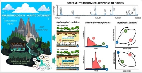
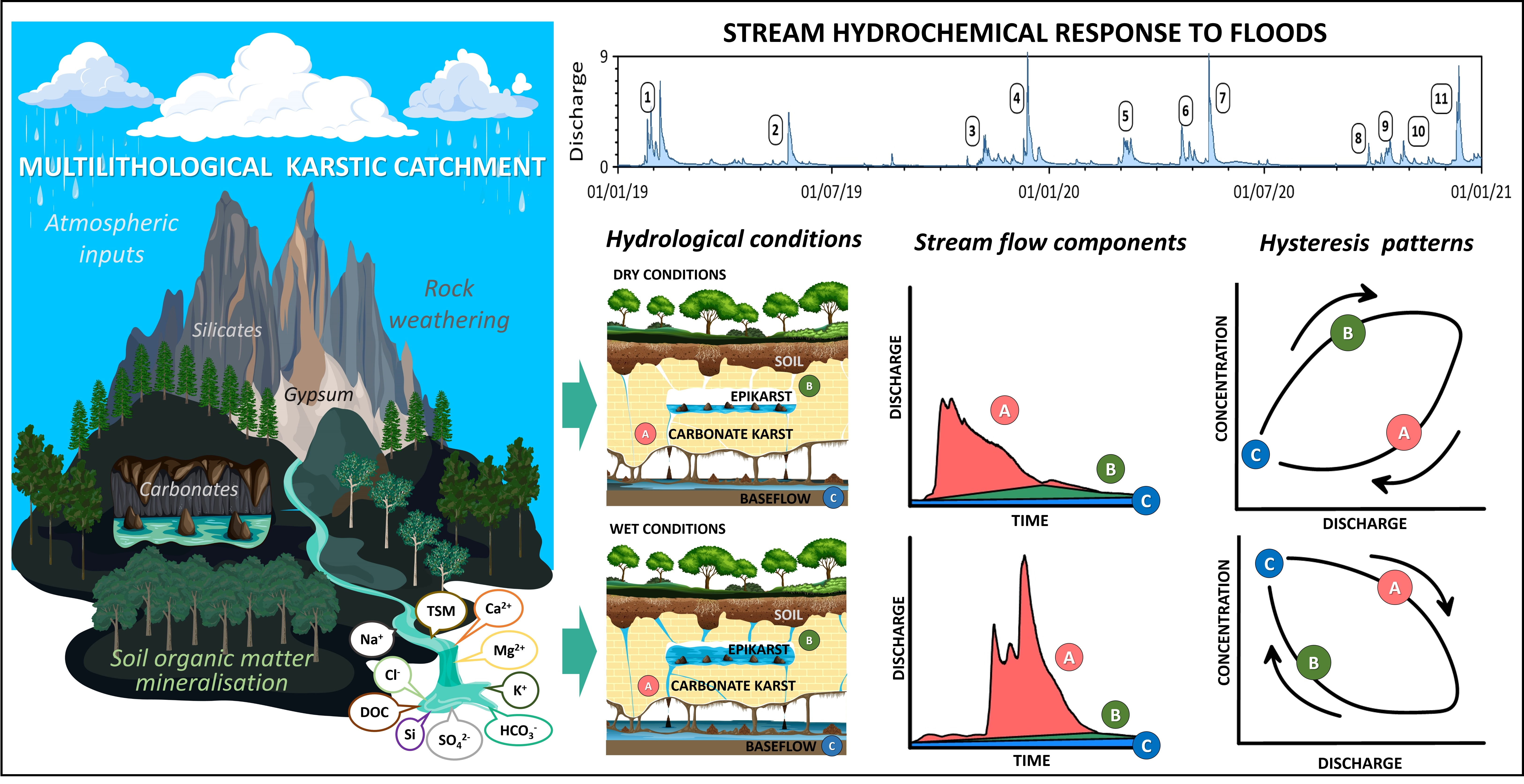
Stream Hydrochemical Response to Flood Events in a Multi-Lithological Karstic Catchment from the Pyrenees Mountains (SW France)

by
Francesco Ulloa-Cedamanos
1,2,3,*,
Anne Probst
1,2,3,
Vanessa Dos-Santos
1,2,3,
Thierry Camboulive
1,2,3,
Franck Granouillac
1,2,3 and
Jean-Luc Probst
1,2,3,*
1
Laboratoire Écologie Fonctionnelle et Environnement, Université de Toulouse, CNRS, Auzeville Tolosane, 31326 Castanet Tolosan, France
2
LTSER Zone Atelier Pyrénées-Garonne, CNRS, Université de Toulouse, 31326 Castanet Tolosan, France
3
LTER Bassin Versant du Baget, SNO Karst, IR OZCAR, CNRS, Université de Toulouse, 31326 Castanet Tolosan, France
*
Authors to whom correspondence should be addressed.
Water 2021, 13(13), 1818; https://doi.org/10.3390/w13131818
Submission received: 28 May 2021 / Revised: 24 June 2021 / Accepted: 29 June 2021 / Published: 30 June 2021
(This article belongs to the Special Issue Water and the Ecosphere in the Anthropocene)

Abstract

:
Hydrological variations hold a significant influence over the water chemistry in the karstic critical zone. In this context, the karstic Baget Catchment (BC) has been monitored at a high resolution over two years at the outlet in order to set up a typology of the flood events. The objective was to assess the multiple streamwater physico-chemical patterns in response to hydrological variations, streamflow component (quick-response, subsurface, and baseflow) and lithological contributions, and biogeochemical processes. The karstic catchment exhibited an impulsive response to flood events in relation to the typical structural and morphological characteristics of the karst. In addition, this response was constrained by the magnitude of the rainfall and the preceding hydroclimatic conditions. The variability of the dissolved load in streamflow was closely associated with the characteristics of the weathered rocks and the hydrological conditions throughout the year. Two simple indicators allow to characterize the concentration–discharge relationships with different hysteresis patterns on a set of floods with various intensities and shapes of the hydrograph and under different hydrological conditions before the flood. Almost all elements exhibited either clockwise loops or more complex behaviors, suggesting a higher overall concentration when the major water contribution comes from the quick-response flow (karst and surface runoff fraction). Besides, the epikarst flushing under dry conditions led counterclockwise hysteresis patterns for calcium (Ca2+) and bicarbonate (HCO3) which revealed an overall chemostatic behavior as a result of carbonate dissolution in the karst. On the contrary, sulfate (SO42−) exhibited the widest relative variation during flooding and showed a significant sensitivity to the dilution process with increasing discharge. For medium flood episodes (Qmax < 4.4 m3·s−1), an overall concentration increase or chemostatic behavior could be observed during the rising limb of the hydrograph. On the opposite, under extreme flood episodes (Qmax > 8.3 m3·s−1) occurring after several rain events, a dilution pattern was noted for all elements originating from rock weathering. Finally, high-frequency sampling during storm events improved the understanding of the factors controlling the hydrochemical dynamic in karstic catchments.

Graphical Abstract

1. Introduction

The ‘critical zone’ is the heterogeneous support zone of the Earth’s surface, in which occur complex interactions between rocks, soils, water, air, and living organisms. It is located between the lower atmosphere and the deepest layer of aquifers, regulating the natural habitat and determining the availability of resources necessary to sustain life on earth [1,2,3]. In the karstic critical zone (K-CZ), the fractured nature of the carbonate rocks and the thin soil cover enhance the water–rock interaction and promote a rapid transfer of surface waters to the underground system, including the epikarst [4]. Epikarst is a discontinuous saturated layer, in which the CO2–H2O–CaCO3 mixed system also occurs; i.e., the carbonate mineral is dissolved by the infiltrated water and the biogenic CO2 stored in the soil [5,6]. Despite some uncertainty, the estimation of the average fluxes of carbonate weathering reaches 1.3 Gt C·yr−1, while the associated CO2 consumption is above 0.1 Gt C·yr−1 at the global scale [7,8].
K-CZ developed in the orogenic context, such as in the Pyrenees Mountains, are considered relevant water supplies [9,10,11], but are also particularly sensitive to anthropogenic activities and climate change [12,13]. Springs and rivers are key vectors of information for understanding and constraining biogeochemical changes in the K-CZ. For instance, local hydrochemistry can elucidate lithological origins and help to understand the streamwater chemistry response face to hydrological changes [14]. Hydrology is closely associated with seasonal changes, which are very marked and contrasted in temperate climates. The dry and the wet (with heavy rains) seasons occur mainly during summer (July, August, and September) and winter and spring, respectively. During the wet season, the forthwith variations due to storms modify the hydrological conditions, leading to dilution processes of some dissolved element concentrations [15]. Based on the water saturation of the hydrological system, dissolved matter can be stored in the epikarst and/or aquifer and/or transported to the outlet through the piston effect [16,17]. High frequency temporal data series are therefore crucial to better understand and constrain the hydrogeological compartment contributions and biogeochemical processes influencing the variation of the hydrodynamic and hydrochemical responses within the K-CZ.
Hydrological, geochemical, and isotopic methods have been used to (i) differentiate the water origins during a stormflow event, i.e., water from rainfall (event water) or from groundwater and soil storage (pre-event water) [18,19,20]; (ii) determine the contribution of the different streamflow components in diverse catchments under various climate conditions [21,22,23,24,25,26]; (iii) elucidate the contribution of different sources to the fluxes of dissolved and particulate matter [27,28,29]; and (iv) assess chemostatic or chemodynamic behaviors at the catchment scale using the relationships between the discharge (Q) and the concentration of dissolved elements (C) [30]. However, few studies have focused on the temporal dynamics of water chemistry using long-term and high-frequency monitoring [31,32,33], particularly in carbonate K-CZ [29,34,35], and even scarcer in multi-lithological K-CZ [17].
The main objective of this study is to assess in a typical multi-lithological K-CZ catchment, the Baget Catchment (BC), the multiple physico-chemical patterns of streamwater in response to hydrological variation, streamflow components (quick-response, subsurface, and baseflow) and lithological contributions, and biogeochemical processes. Based on a high-frequency survey (continuous measurements using a multiparameter probe and water sampling every two hours) of the streamwater hydrochemistry, particularly during flood events at the outlet of the BC, the objectives of this paper are to (i) investigate the sensitivity (chemostatic or chemodynamic responses) of the streamwater chemistry to sudden hydrological variations; (ii) quantify the contribution of each streamflow component for different rainstorm conditions; and (iii) elucidate the dominant controlling factors of changes in hydrochemistry during storm events.
The BC, located in the French Pyrenees Mountains, has been monitored since the 1970s, and has a long-term survey hydrogeochemical database [17]. In addition to the background survey, a high-frequency flood survey of the multi physico-chemical parameters has been running since 2019, based on continuous measurements and instantaneous sampling, allowing to set up a typology of flood events.
The supporting hypotheses were that (i) the response of the major dissolved elements to flash floods would be diverse according to the multi-lithological characteristics of the BC, as some elements will increase in concentration while others will decrease (dilution) or remain unchanged (chemostatic behavior); (ii) the major streamflow component would be the quick-response flow (karst and surface runoff fraction) due to the open fractures and developed drainage networks, typical of a karstic system; and (iii) the environmental characteristics would drive the water chemistry, primarily the drainage intensity and the lithology with their spatial distribution and temporal activation of their sources, the biogeochemical processes, the hydroclimatic variation, and the antecedent hydrological conditions.

2. Materials and Methods
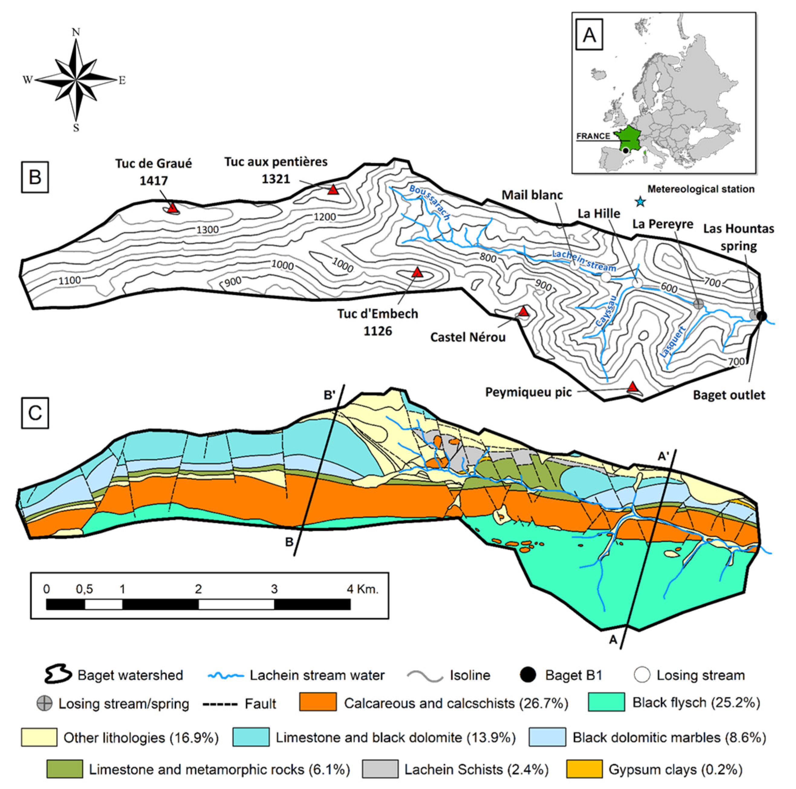
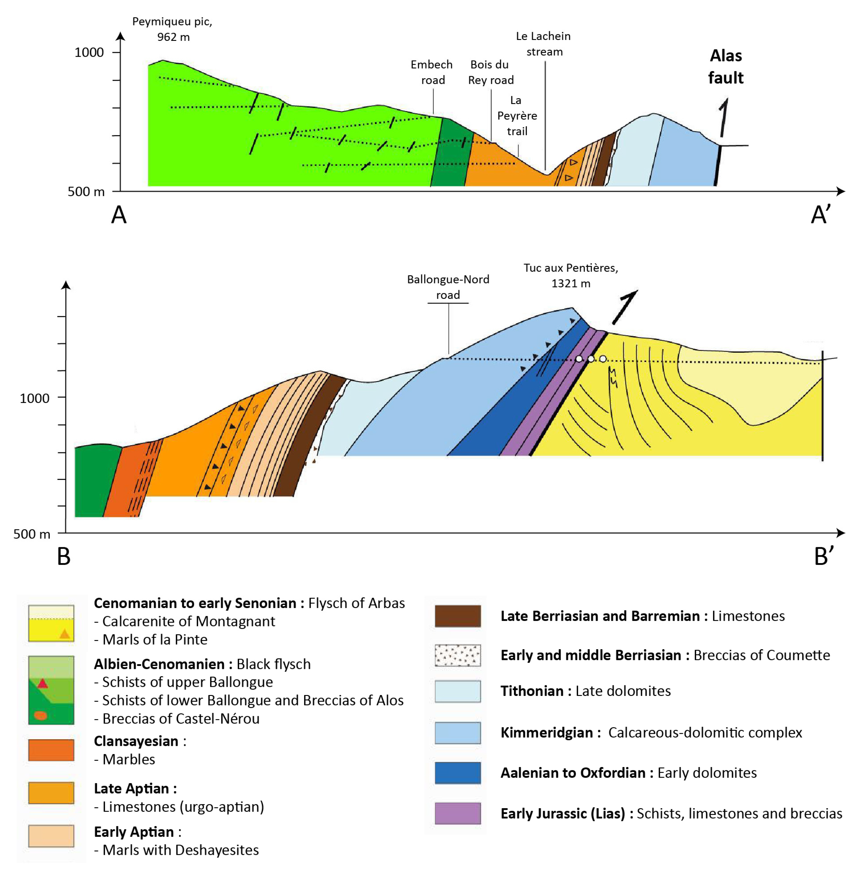
2.1. Study Area

The BC (42°57′420″ N, 0°58′30″ E) is a small (13.25 Km2) forested karstic catchment with an altitude range between 498 (at the outlet) and 1417 m a.s.l. The BC is located in the lower part of the Pyrenees Mountains, in the Southwest of France (Figure 1A). It is drained in its middle and lower parts by the Lachein stream. Mangin [36] described the BC as more karstified in the upper part of the catchment than downstream. The presence of non-karstified terrains in the lower part delays the water infiltration to groundwater.
The BC is influenced by an Atlantic oceanic climate coupled with a clear mountainous tendency. The daily mean air temperature registered at the closest Meteo-France meteorological station situated 8.3 km downstream from the outlet of BC (Saint Girons, 43°00′19″ N, 1°06′25″ E) is 11.8 ± 6.3 °C (from January 1960 to December 2018, N = 21,531). The rainfall regime is bimodal with runoff peaks of the Lachein streamwater in early winter (end of December) and late spring (around May) [17]. During the hydrological year 2019–2020 (from October 2019 to September 2020), 60% of the annual rainfall (1713 mm·yr−1) occurred from November to December and from March to May (wet season).
The Lachein stream is fed by three small perennial tributaries draining impermeable surfaces (from upstream to downstream): the Boussarach creek on the left bank and the Cayssau and Lasquert creeks on the right bank. The BC is characterized by losses and temporary springs (Figure 1B) feeding the karstic network up to 498 m altitude where the main perennial spring, Las Hountas, defines the limit between the temporary stream of Lachein (dried up during the low water level period, discharge at the outlet <0.15 m3·s−1) and the permanent Lachein stream. The latter joins the Lez River 1 km to the east. The mean annual discharge at the outlet, located 60 meters downstream of Las Hountas, is 0.48 m3·s−1; i.e., a specific discharge of 36 L·s−1·Km−2 [37]. As the system is flooded, overflows appear and surface runoff is lost at different levels depending on the magnitude of the flood event (Figure 1B). During flood conditions, the surface runoff closely follows the evolution of the flood event. However, in spring, surface runoff emerges at the slightest rainfall and disappears after the rainy episode, unlike in winter or late summer, when it shows rather low discharge values [36].
The BC landscape is mostly covered by forests (67% of the basin area in 2019), followed by grasslands located near to the outlet and some pastures in the upper part of BC. Despite its small drainage area, the BC includes almost all the geological formations of the central North Pyrenean zone owing to the major North Pyrenean fault, called Alas (Appendix A) [38]. This catchment lays on calcareous formations of the Jurassic and Cretaceous represented by a band of limestone bordered to the north and south by impermeable silicate rocks (black flysch in the south and breccia—metamorphic rock—in the north, both Na-rich [39] and from the Cretaceous period) and by dolomitic outcrops from Jurassic in the northern upper section bordered also by silicate rocks (Cretaceous flysch of Arbas—other lithologies—and Paleozoic Lachein schists) (Figure 1C, Appendix A). Sulfide minerals (meanly pyrite, FeS) are associated as a minor phase to limestones and flyschs [14,36], while sulfate minerals (mainly gypsum, CaSO4·2H2O) from the Upper Triassic represent only 0.2% of the BC surface area.
The experimental BC is part of the French Karst Observatory Network (SNO Karst) [40] and belongs to the observatories of the French Research Infrastructure called OZCAR (Observatoire de la Zone Critique: Application et Recherche) [41], included in the European Research Infrastructure eLTER (Long Term Ecosystem Research in Europe) [42,43].

2.2. Sampling and Analysis

Hydrochemical Measurements

The hydrochemical survey was carried out at the BC outlet (Baget outlet, Figure 1B): (i) a weekly sampling between 1978 and 2006 by the CNRS laboratory of Moulis [44]; (ii) every 6 months by BRGM Occitanie [45] from 2007 to 2014; and (iii) a biweekly sampling that started in 2014 and is currently ongoing by the Laboratoire écologie fonctionnelle et environnement [17]. In addition, high-frequency sampling was conducted between February 2019 and December 2020 during the flood events. Rainfall and rainwater samples were also collected monthly from September 2019 to December 2020 at the meteorological station of Balagué (42°58′06.5″ N 1°00′39″ E, elevation 658 m, Figure 1B). Rainfall between January 2019 and August 2019 was calculated using the daily rainfall registered at the closest Meteo-France meteorological station of St. Girons (elevation 414 m), situated 8.3 km downstream from the outlet of BC. The very significant relationship (R2 = 0.80; p < 0.001; n = 365, with a slope of 1.39) between the rainfall at Balagué and at St. Girons stations was used for this calculation.
The physico-chemical parameters, such as water temperature (Water T°), specific conductivity (Cond), dissolved oxygen (DO), and pH, were measured at the time of sampling using a portable multi-parameter (WTW probe, Xylem Analytics Germany Sales GmbH & Co., Weilheim, Germany) at the Baget outlet. This site is equipped with a mechanical limnigraph (OTT 20 1/5; Loveland, CO, USA) and a float-type water-level sensor (OTT Thalimedes; Loveland, CO, USA). Several gauges served to plot the rating curve and thus estimate the discharge from the water height. Discharge data at the outlet since 1968 are freely accessible [46]. In addition, since April 2014, water level and different physico-chemical parameters (Water T°, pH, Cond, Turbidity, DO, nitrate and chloride) were measured continuously at a high frequency (10-minute interval) in the mid-depth of the water column (at the outlet) using a multi-parameter probe (YSI 6920V2-01, YSI Incorporated, Yellow Springs, OH, USA) equipped with multiple sensors and an atmospheric pressure correction. Moreover, during the study period (2019–2020), water samples were collected every two hours using an automatic sampler and analyzed in the laboratory.
Water samples were collected in a clean and dry 1 L HDPE bottle, triple rinsed with streamwater before sampling, and stored in darkness at 5 °C until analyses. All samples were filtered using Millipore 0.22 µm cellulose nitrate membranes. Alkalinity was determined using a standard acid titration method with HCl 0.02N and a Metrohm titrant (716 DMS Titrino, Metrohm, Riverview, FL, USA). Major anion concentrations (SO42−, NO3, and Cl) were analyzed by ion chromatography (Dionex apparatus ICS 5000+, Thermo Fisher Scientific, Waltham, MA, USA). Major cation (Ca2+, Mg2+, Na+, and K+) and silica concentrations were measured using an acidified sample with 16N HNO3, later analyzed by an inductively coupled plasma optical emission spectrometer (ICP-OES; Iris Intrepid II XLD, Thermo Electron, Thermo Fisher Scientific, Waltham, MA, USA). The total dissolved solids content (TDS) was calculated by adding up all the dissolved species mentioned above. Dissolved organic carbon (DOC) was measured on a Shimadzu TOC 5000 analyzer (Shimadzu Corporation, Kyoto, Japan), coupled to the CO2 detection by an infrared gas analyzer (NDIR).
Regarding the quality assurance (QA), the protocols for sampling, filtration, pre-treatment, and storage of the stream- and rainwater before analysis were always controlled. Concerning the quality control (QC), all the methods of analysis were controlled following French (NF), European (EN), and international (ISO) standards. In addition, the physico-chemical analysis laboratory of the Laboratoire écologie fonctionnelle et environment takes part every year to the ICP-Water Intercomparison with the Norwegian Institute for Water Research (NIVA), which follows a QA/QC procedure.

2.3. Data Treatment

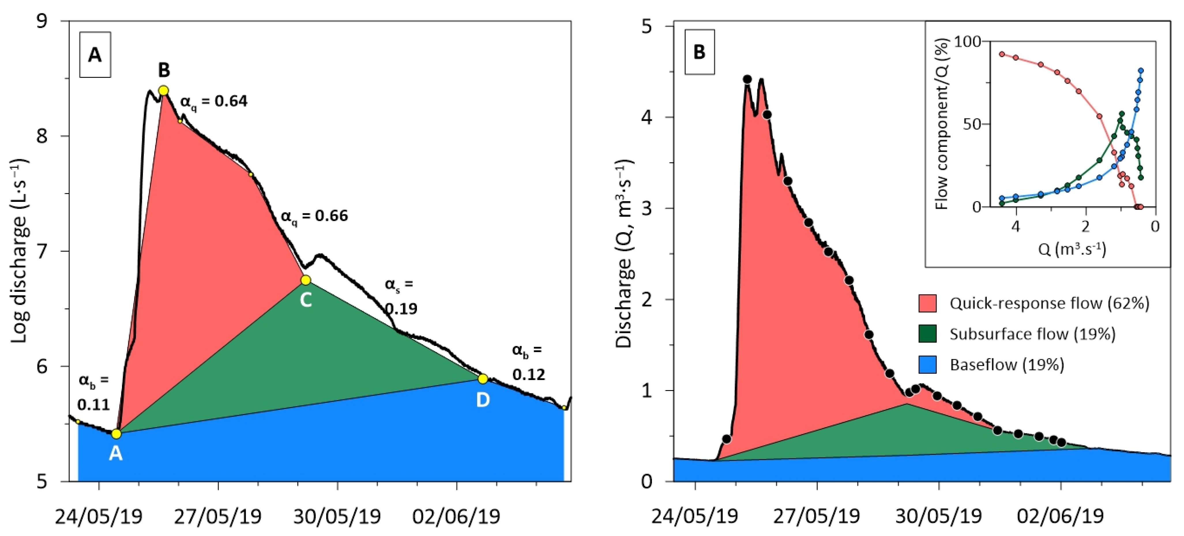
2.3.1. Hydrograph Separation Method

The streamflows were split into the quick-response flow (karst and surface runoff fraction), the subsurface flow (epikarst and infiltration fraction), and the baseflow (groundwater fraction) (Figure 2).
The onset of a storm period was established when the discharge increased suddenly, exhibiting a marked inflection (Point A, Figure 2A). This sudden change was assessed when the discharge change rate (DCR, Equation (1)) was greater than 100%.
D C R = Q i + 1 Q i / Q i 100
where Qi and Qi+1 are the daily discharge at time-step i and i + 1. The end of the storm period was determined when the DCR was greater than −20% and the base discharge was lower than 300 L·s−1 in BC (Point D, Figure 2A). Moreover, small floods leading to discharge variation only within ±1 m3·s−1 were not considered.
The quantitative analysis of the recession curves is derived from the research of Maillet [47], who indicated that the recession curve of the hydrograph during a storm period can be characterized by an exponential decrease of the discharge (Equation (2)), suggesting a linear relationship between the piezometric head and flowrate [48].
Q t = Q 0 e α t
where Qt is the instantaneous discharge at time-step t (in days in our study), Q0 is the initial discharge at time zero, and α is the recession coefficient. This coefficient depends on the characteristics of each flow associated with the reservoir it drains, allowing to differentiate the different streamflow components on the basis of their “α” coefficient.
The hydrograph separation method proposed by Probst [24,49,50] was adapted for karst systems, assuming that the quick-response flow (karst and surface runoff fraction), the subsurface flow (epikarst and infiltration fraction), and the baseflow (groundwater fraction) occur simultaneously. The first step is to transform the curves of the hydrograph into straight lines by using the logarithm of the discharge. Then, the descending limb corresponding to the recession period is divided into three straight lines with different slopes through the determination of two inflection points (points C and D, Figure 2A corresponding to the end of the quick-flow and subsurface-flow contribution, respectively [24]. Then, the separation line between the subsurface runoff with the quick-response runoff and with the baseflow was drawn by connecting points A–C and A–D, respectively.

2.3.2. Analyses of C-Q Relationships

The temporal variations in both discharge and concentrations can be analyzed also using the relationships between concentrations and discharges, which generally follow a power-law function (Equation (3)) [51]:
C i = a   Q i b
where Qi and Ci are the instantaneous discharges and dissolved element concentrations, respectively, at time-step i. The exponent b is a useful indicator of the chemodynamic features of the dissolved element behavior. If b < 0, the dilution effect produced by Q is the major regulator on C; if b = 0, C exhibits a chemostatic behavior, without influence of Q variation; if b > 0, an enrichment takes place on the solutes when the discharge increases.

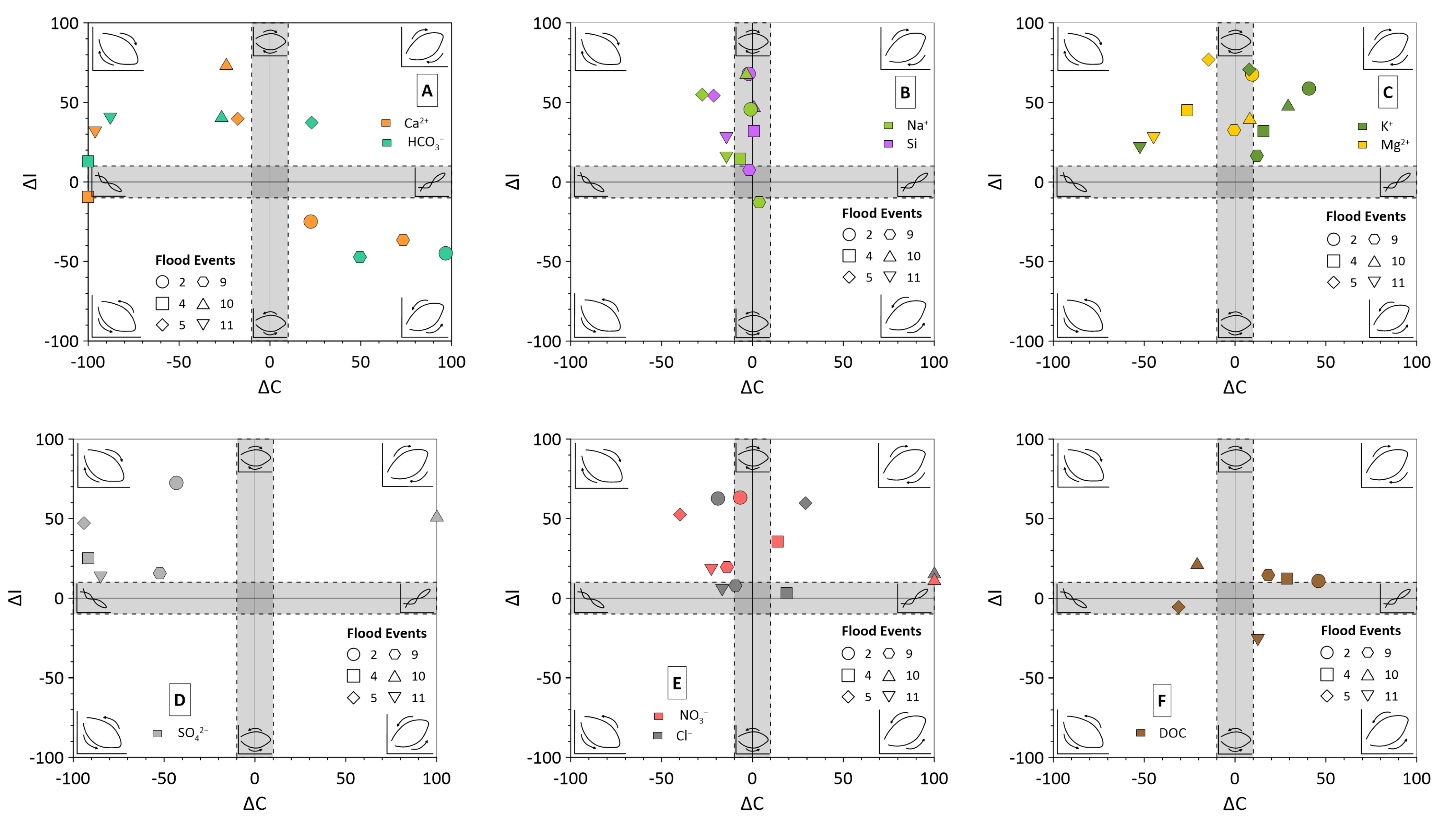
2.3.3. Hysteresis Analyses

During a flood, the C-Q relationship can take the shape of a straight line or a loop, called hysteresis [52]. This hysteresis reflects the different concentration responses to the same discharge during the rising and falling limbs of the hydrograph.
To characterize the hysteresis patterns, we used two simple descriptors that describe the relative changes in dissolved concentrations (ΔC), the direction of rotation, and the relative amplitude of the loop pattern (ΔI).
Δ C = C p C b C p × 100 ,   i f   C p > C b   C p C b C b × 100 ,   i f   C p < C b
where Cb and Cp are the instantaneous dissolved element concentrations at the base flow and during the peak flow of the flood event, respectively. Positive and negative values of ΔC indicate a concentration increase or dilution, respectively [53]. ΔC values ranging between −10 and 10 can be considered as corresponding to a neutral response discharge increase.
The normalized data were also used to compare the hysteresis behavior of each parameter within and between different flood events (Equations (5) and (6)).
Normalized   Q i = Q i Q m i n / Q m a x Q m i n
Normalized   C i = C i C m i n / C m a x C m i n
where Qi and Ci are the instantaneous discharge and dissolved element concentrations at time-step i, respectively. The Qmin, Qmax and Cmin, Cmax correspond to the minimum and maximum values of the discharges and concentrations during a complete flood event, respectively.
The relative amplitude of the loop pattern (ΔI) can be calculated as follows:
Δ I   % = C i R L n o r m C i F L n o r m × 100
where Ci−RL_norm and Ci−FL_norm refer to the normalized concentrations on the rising limb (RL) and on the corresponding falling limb (FL) of the hydrograph, respectively, for each 25% increase in discharge [54,55]. Positive and negative values of ΔI indicate clockwise or counterclockwise loops, respectively. For ΔI values between −10 and 10, one can consider that there is no loop or ambiguous rotational response to increasing discharge.

2.3.4. Method of Flux Calculation

The total flux (Ftotal) was estimated by adding all fluxes corresponding to each flood event, estimated between two sampling intervals (i to i + 1) using the discharge-weighted average concentration (Cj) and the water volume (Vj), according to the following equations:
C j = i i + 1 C i   x   Q i i i + 1 Q i ,
V j = i i + 1 Q i   x   t i + 1 t i 2 ,
F t o t a l = j n C j   x   V j ,
with Ci: concentration at time i; Qi: discharge at time i; and Vj: volume of water flow between i and I + 1.

3. Results

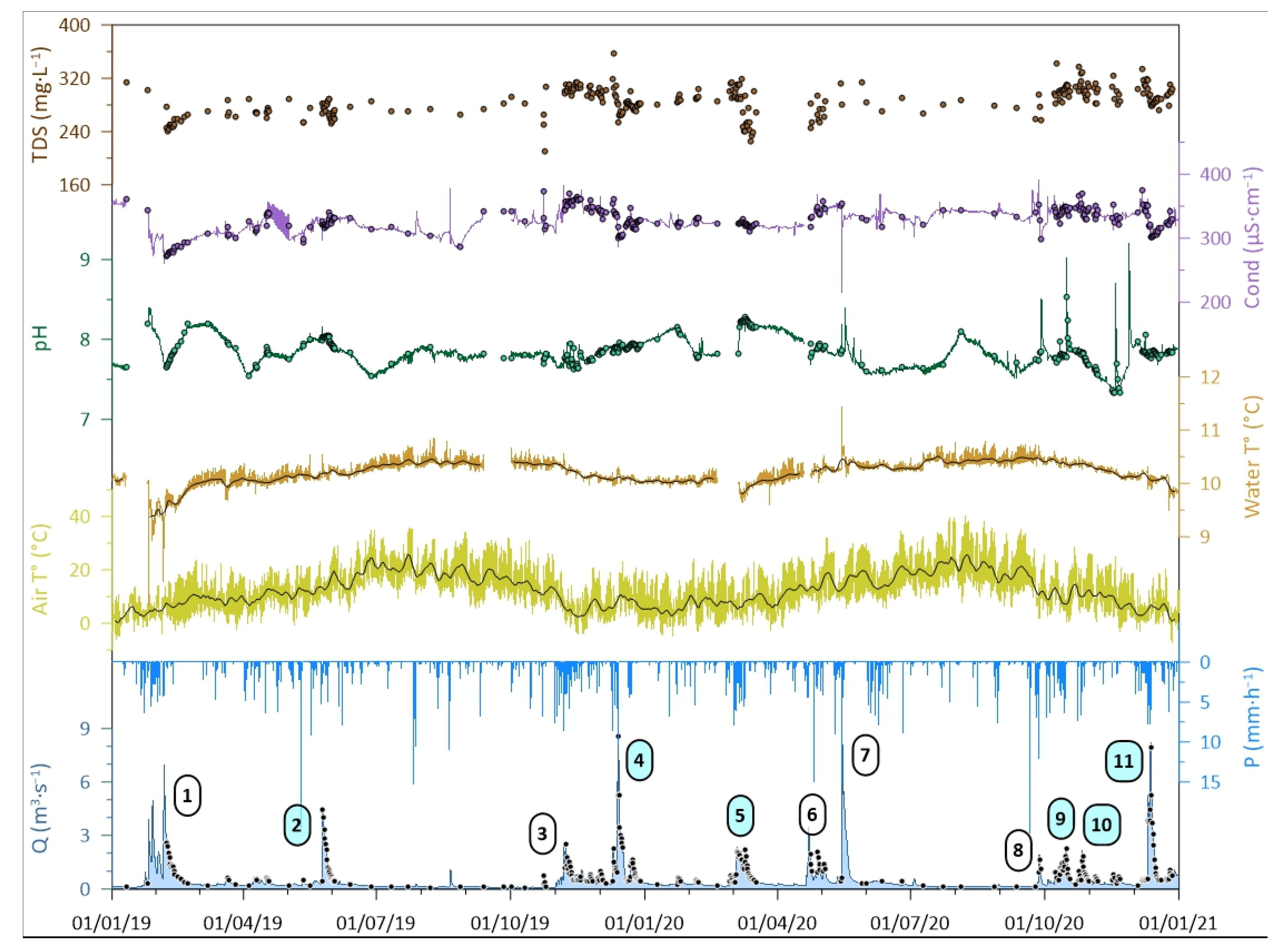
3.1. Hydrochemical Survey during the Period 2019–2020

The summary of the hydrochemical and physicochemical characteristics of the streamwater are reported in Table 1. All parameters reacted to different extents to the hydrological variations, as indicated by their coefficient of variation (CV = σ/ X ¯ ).
The discharge, water, and air temperatures (Figure 3) exhibited an obvious seasonality during the two years of survey, but their CV is very different: the highest variation was for the discharge (CV = 1.03) and the lowest one was for the water temperature (CV = 0.02). The study period is 20% wetter (Q = 0.53 m3·s−1) compared to mean of the last 40 years (Q = 0.44 m3·s−1) [17]. The total rainfall amount was 1543 mm and 1632 mm for the years 2019 and 2020, respectively. The mean volume of rainfall was 21.0 × 10⁶ m3 per year. Open field precipitation is circumneutral, and very low concentrated in the major dissolved elements (<25 µmol·L−1). Na+ and Cl are the dominant ions whereas the Mg2+, K+, SO42−, and NO3 concentrations are very low (mean concentration <6 µmol·L−1, Appendix B).
The streamwater in BC is mildly alkaline and pH showed low fluctuations (7.9 ± 0.2). The water temperature is highly stable (10.1 ± 0.2 °C) throughout the study period. Conductivity is related to total dissolved solids (R2 = 0.4, p < 0.01). The mean concentration of the different elements in the streamwater exhibited the following abundance order during the study period: for cations, calcium (Ca2+, 88.8% of total cationic concentration in µeq·L−1) >> magnesium (Mg2+, 9.7%) >> sodium (Na+, 1.1%) > potassium (K+, 0.4%); and for anions, bicarbonate (HCO3, 93.5% of total anionic concentration in µeq·L−1) >> sulphate (SO42−, 4.4%) > chloride (Cl, 1.3%) > nitrate (NO3, 0.8%). The predominance of Ca2+, Mg2+, and HCO3, which represent 96% of the ionic charge, is related to the dominant carbonate lithology of the BC [14,17]. The discharge-weighted mean concentration of sulphate has significantly decreased during the study period (0.15 µeq·L−1) compared to the period 1978–2018 (0.35 µeq·L−1) [17]. In addition, Ca2+ and HCO3 were the most stable ions, while SO42−, K+, NO3, and DOC exhibited a higher CV (Table 1). The HCO3 is the dominant species of DIC according to the water pH and its concentration is much higher than the world river average concentration of 850 µmol·L−1 [56].
The concentrations of the major elements, represented by TDS, show significant temporal variations in the BC (Figure 3). The average TDS (285.5 mg·L−1) is around 3 times the world river TDS average (97 mg·L−1) [56]. Compared to other rivers draining carbonates in the world, the mean TDS in BC is higher than those of the Wujiang River in the Yunnan-Guizhou plateau (265 mg·L−1) [35], the Ganges and Indus rivers in the Himalayas (164 mg·L−1) [57,58], or the Mackenzie River in the Rocky Mountains (160 mg·L−1) [59]. However, compared to rivers in temperate karst terrains, the TDS values measured in BC are similar to those measured in rivers of the Alps Mountains (253 mg·L−1 during spring and 378 mg·L−1 during winter) [60] and lower than in the Jura Mountains (378 mg·L−1) [61].
The Net Inorganic Charge Balances (NICB % = 200 × (TZ+ − TZ)/ (TZ+ + TZ)) between the sum of anions (TZ) and the sum of cations (TZ+) (both in meq·L−1) are on average 4.0 ± 3.5%, with 70% of the samples having an NICB of less than 5%. This indicates that the contribution of unanalyzed ions, such as organic anions, play a negligible role in the water chemistry.

3.2. Hydrochemical Features of Flood Events

3.2.1. Flood Hydrological Characteristics

During the study period, eleven hydrological events were observed (Figure 3, Table 2). The duration of these events was variable but closely within the range of influence on discharge, between 10 and 20 days, as shown by Mangin [36] for the BC.
The contrasted flood events, 2, 9, 10, and 11 (Figure 3, Table 2), were analyzed in more detail. These flood events were chosen based on (i) the period of the hydrological year: beginning of the hydrological cycle (floods 9 and 10), first high-water level period (flood 11), and the last flood of the hydrological cycle (flood 2); (ii) the intensity/magnitude of the flood event reflected by the differentiated discharge peaks (2.13, 2.29, 4.42, and 8.25 m3·s−1, respectively) and specific discharges (44.6, 63.7, 92.5, and 165.3 mm, respectively); (iii) similar discharge values (Qmean-24h) preceding the flood event; and (iv) the potential influence of past and/or successive floods.
During the last three studied flood events (9, 10, and 11), the pH of the open field precipitation was between 6 and 7, and Ca2+ is a major element in the rainwater together with Na+ and Cl ions (<25 µmol·L−1). Unlike flood events 10 and 11, flood event 2 followed a relatively dry period straight after a major flood, such as for floods 1 (discharge peak of 7.0 m3·s−1) and 4 (discharge peak of 9.4 m3·s−1). Flood 9 was preceded by the smallest flood identified (discharge peak of 1.9 m3·s−1 with a total duration of 5 days) whose influence on the water chemistry was minor.

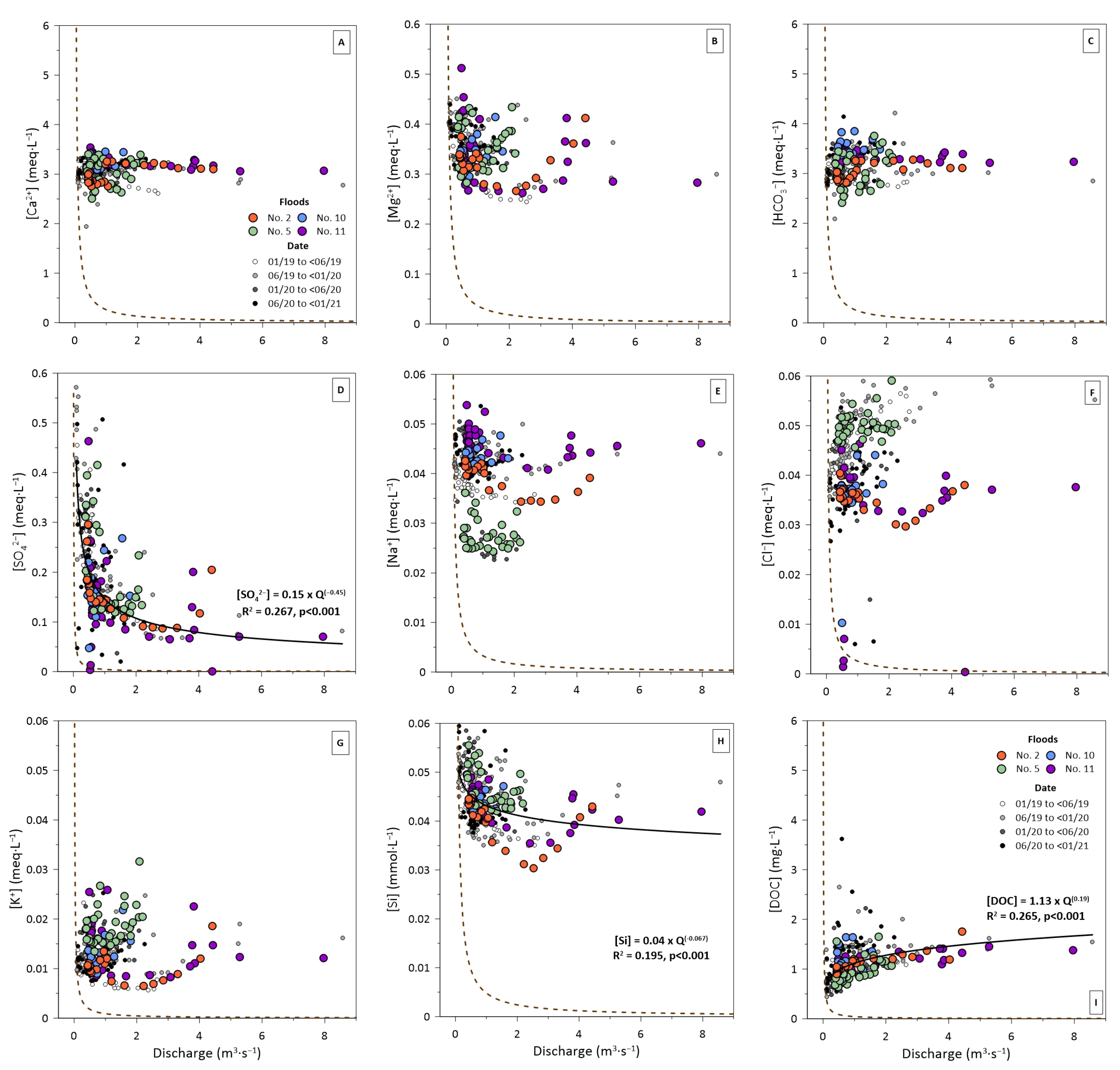
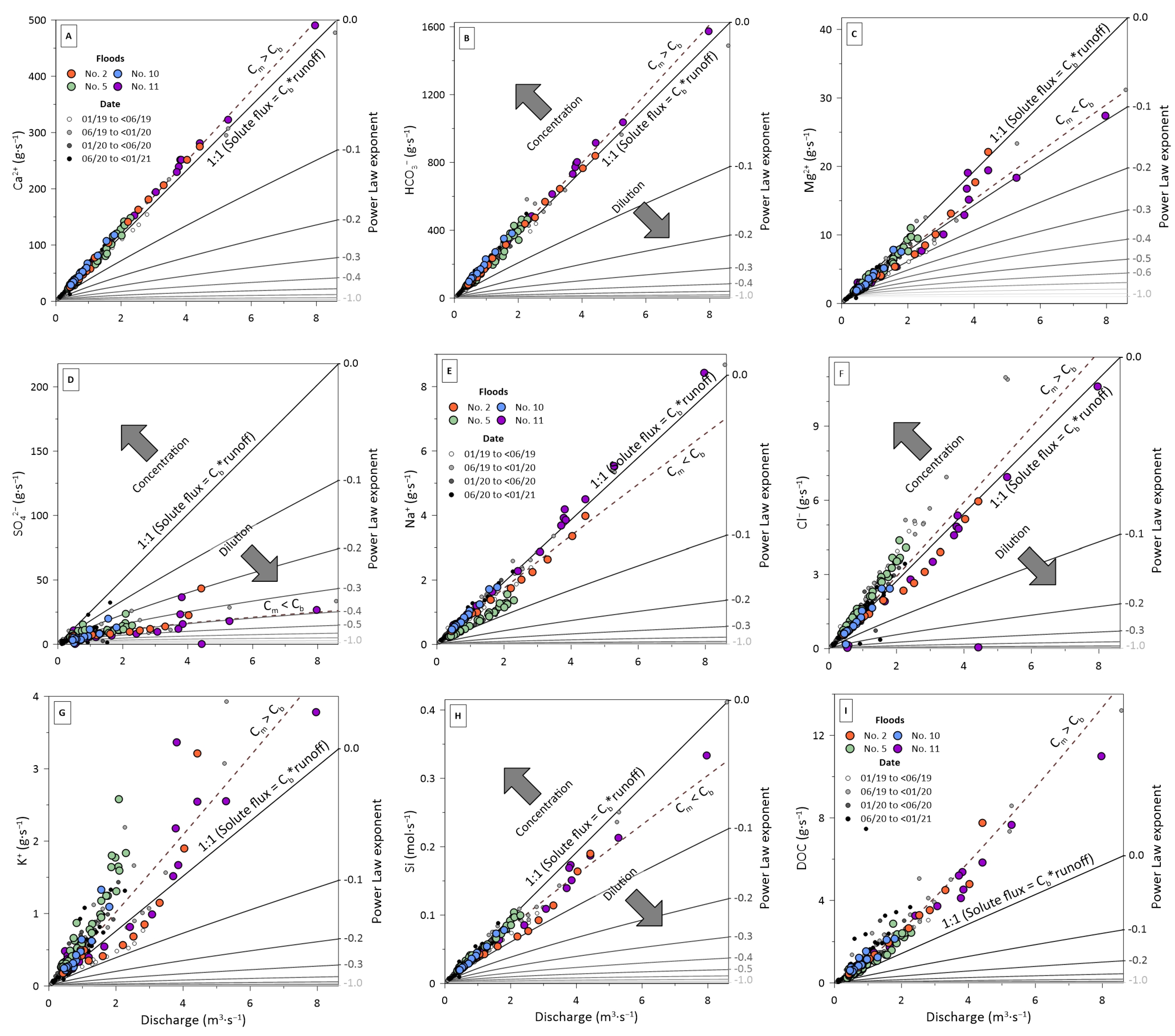
3.2.2. C-Q Relationships

The control of discharge over the dissolved element concentrations can be observed by comparing the temporal variations inof TDS and of discharge (Figure 3), and by the relationships between the concentrations and discharges (C-Q) (Figure 4).
The C-Q relationships indicated consistent patterns between some elements, such aslike Ca2+ and HCO3 inon one way, and Cl and K+ inon the other way. A similar pattern was also detected between Mg2+, Si, and Na+, buteven slightly less evident. Nevertheless, the global relationships were not significant for Ca2+, HCO3, Cl, K+,+ and NO3, showing globally a chemostatic behavior during the whole period. On the contrary, the C-Q relationship for SO42− is significant and follows a dilution curve. The slope (b = −0.45) of the power-law function (C = aQb) for SO42−tends to a pure dilution curve (b = −1). The Mg2+ (b = −0.07), Si (b = −0.07), and Na+ (b = −0.05) concentrations underwent a significant dilution. The DOC was the only parameter with a clear enrichment with increasing discharge, exhibiting a positive significant relationship (b = 0.19). Among those global trends, specific patterns can however be observed during the flood events (Figure 4). For instance, flood events 10 (October) and 11 (December) exhibited concentrations of Ca2+ and HCO3 much higher (Figure 4) than during flood events 5 (February) and 2 (May). Flood event 5 displayed the lowest concentration of Na+ and DOC but the highest concentration of Cl, K+, and Si (Figure 4).

3.3. Specific Patterns of Representative Flood Events

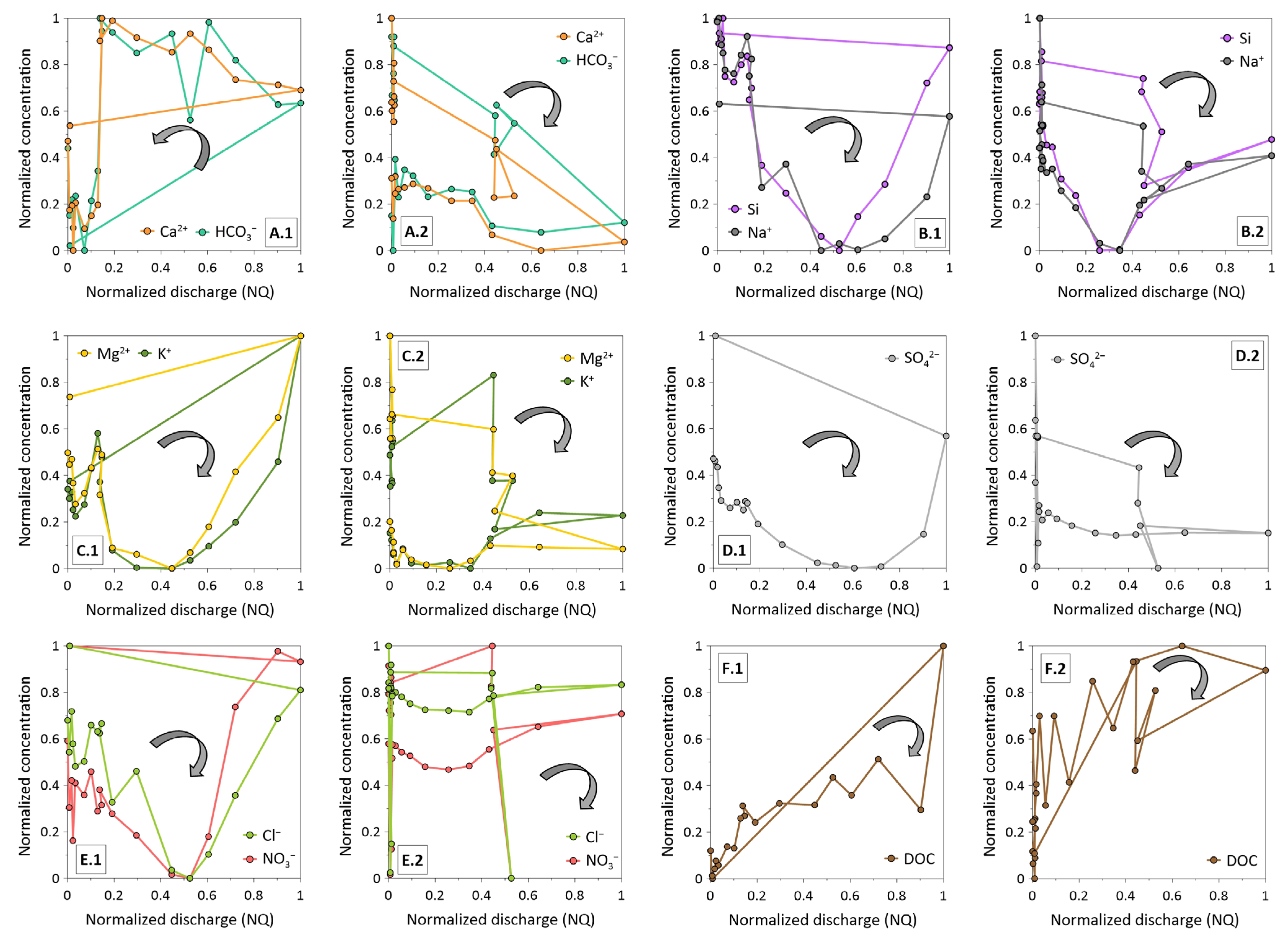
3.3.1. C-Q Patterns for Representative Floods

Considering all the data together, no clear relationships could be observed between C and Q (Figure 4), but single flood events exhibited more obvious C/Q patterns (Figure 5). The overall patterns can be illustrated for flood events 2 and 11 (Figure 5), which in essence represented similar initial hydrological conditions observed for flood 9 and for floods 4, 5, and 10.
Loop trajectories of Ca2+ and HCO3 exhibited clockwise (floods 4, 5, 10, and 11) but also counterclockwise responses (floods 2 and 9). For the other dissolved elements, loop trajectories displayed clockwise responses or more complex behaviors, such as a figure-of-eight shape (Figure 5).
A decrease in Ca2+ and HCO3 concentrations with increasing discharges was observed during the major peak flow (8.3 m3·s−1) of flood 11. Similar behavior was observed during the major peak flow (9.4 m3·s−1) of flood 4. For the other floods, such as flood 2, a slight variation was observed in the Ca2+ and HCO3 concentrations (Figure 5A).
During flood events 2 (peak Q = 4.4 m3·s−1) and 11 (peak Q = 8.3 m3·s−1), the Na+, Si, Mg2+, and K+ concentrations showed a similar trend during the recession period: decreasing concentrations up to about 2.5 m3·s−1 and then increasing concentrations (Figure 4C and Figure 5B). This behavior was also observed for flood 4, unlike floods 5, 9, and 10 whose peak discharges were lower than 2.5 m3·s−1.
An overall dilution was observed for the SO42− concentration (Figure 5D), except during the first peak of the minor flood event 11 as well as in flood 5 and 10 (Qpeak < 1.5 m3·s−1). The DOC concentration showed a clear increase with discharge for all flood events (Figure 5F), except for flood 10.

3.3.2. Typology of Flood Events

Based on the hydrological events sampled in BC, the main hydrochemical patterns were characterized during flood events, depending on the initial hydrological conditions before the flood, the intensity, and the shape of the flood hydrograph (Table 3).
The initial dry conditions correspond to long periods of very low rainfall and relatively high evapotranspiration. The floods occurring after these dry conditions are typically of short duration and intensity. Their chemical response to increasing discharge is characterized by slight anti-clockwise variations for the Ca2+ and HCO3 concentrations and clockwise variations for Na+, Si, and Mg2+. The SO42− concentration is systematically diluted while K+ and DOC are concentrated. Cl and NO3 exhibit different clockwise behaviors, depending on the intensity of the flooding.
During the initial wet conditions, the C-Q relationships displayed an overall dilution (except for DOC) if the intensity of the flood event is extremely high associated with a long period of intermittent rainfalls before the major peak. Under low flooding intensity, Ca2+, HCO3, Na+, Si, and Mg2+ concentrations displayed a clockwise hysteresis with non-significant concentration variation. Meanwhile, SO42−, K+, Cl, and NO3 showed a concentration increase response, unlike the DOC concentration.
Based on the C/Q patterns (Figure 5) and on the typology of flood events (Table 3), we selected the representative flood events 2 and 11 for more in-depth analysis. These two floods represent the hydrological and hydrochemical responses under dry and wet hydrological conditions, respectively. Besides, the shapesshape of these hydrographs are less complex and allows better separation of the different streamflow components.

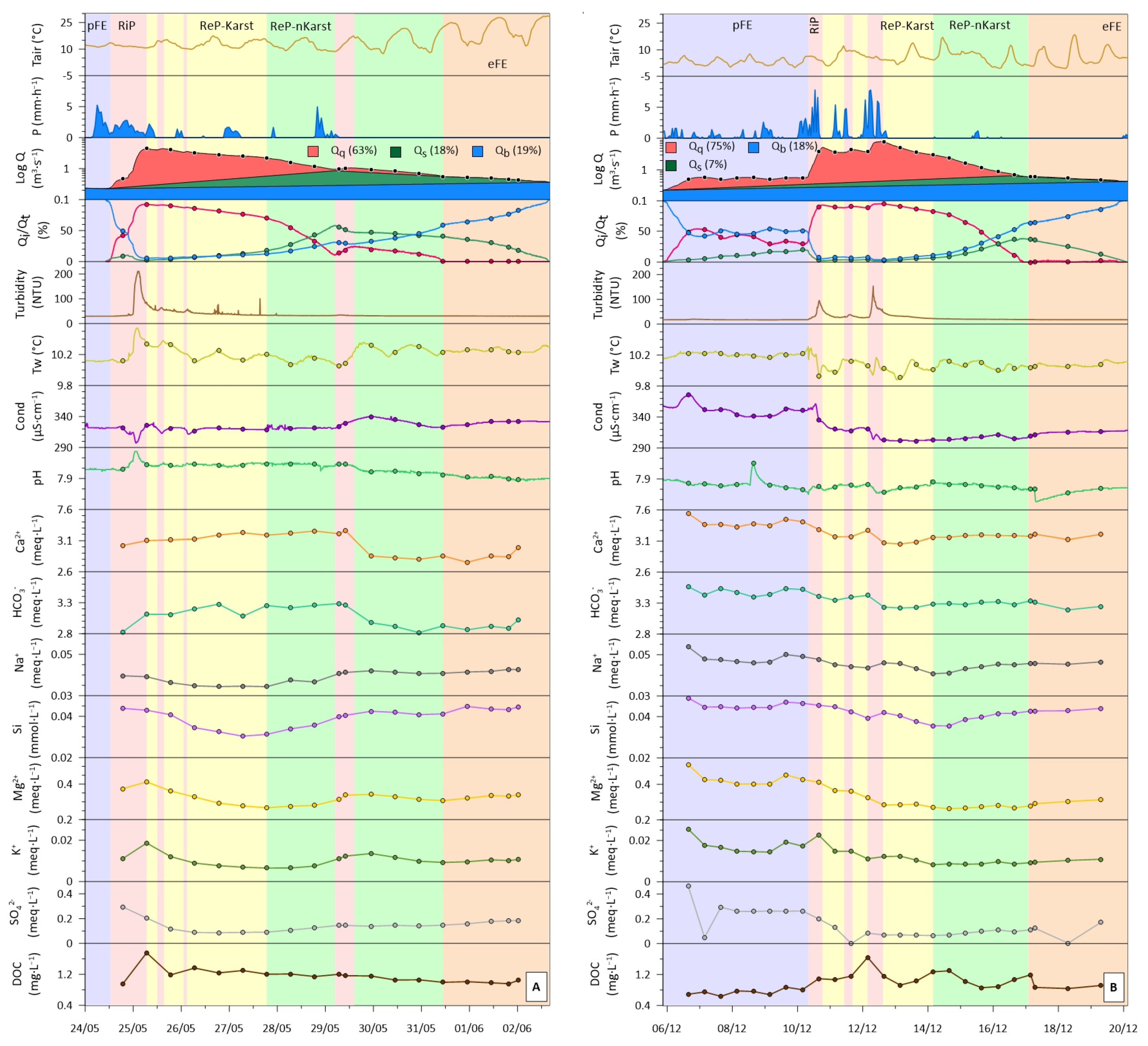
3.3.3. Hydrochemical Patterns and Streamflow Components during Floods 2 and 11

HydrologicalThe hydrological event 2 (Figure 6A) started on 24 May and ended 10 days later, with most rainfall on the first day. The major peak flow was reached 25 hours after the rainfall peak in hourly precipitation (5.2 mm on 24 May, 06:00). Several small rainfall events perturbed the discharge during the recession limb of the flood event.
The hydrograph separation of flood event 2 (Figure 2A and Figure 6A) exhibited three distinct recession coefficients (α), respectively, for the quick-response flow (αq: 0.64 to 0.66), the subsurface flow (αs: 0.19), and the baseflow (αb: 0.11 to 0.12). The analysis of the other flood events in BC (Figure 3) showed that the different α values (with t in days) ranged between 0.40 and 0.80 for αq, from 0.10 to 0.20 for αs, and between 0.04 and 0.12 for αb.
During the first part of the recession, the quick flow-response represented the main contribution (>50%) to streamflow during one-third (3.5 days) of the flooding episode up to a stream discharge higher than 1.5 m3·s−1. Its contribution decreased progressively while the subsurface flow became dominant for a stream discharge close to 1 m3·s−1 (Figure 2B, Figure 6A). Likewise, the baseflow dominance corresponds to a stream discharge lower than 0.65 m3·s−1.
Water temperature and turbidity increased (up to 0.4 °C and 180 NTU, respectively) with increasing discharge and then returned to the initial values. The increasing discharge caused a sharp decrease in conductivity (up to a minimum of 297 µS·cm−1) followed by a return to previous conditions, except after the last rainy episode when it showed a positive synchronism as discharge increases (29 May). The pH presented a small increase with the main discharge peak and remained stable until 29 May, and then it gradually decreased. During the first part of the falling limb, the Ca2+ and HCO3 concentrations and the molar ratio Ca/Na increased, unlike the Mg2+, SO42−, and Si concentrations and the molar ratio SO4/HCO3. The concentrations of the first group of elements decreased or stabilized till the last rainfall episode of 29 May, after which the Ca2+ and HCO3 concentrations decreased sharply. For the second group of elements, they increased from 27 May onwards, when the contribution of the quick-response flow decreased markedly (Figure 6A). A peak in the DOC concentration is observed with the peak flow, followed by a slight and regular decrease.
Hydrological event 11 started on 6 December till 20 December 2020 (Figure 6B). During this event, two minor flow peaks preceded the major flow peak. The first flow peak was reached 6 hours after the first highest hourly rainfall (7.8 mm on 10 December, 17:00), while the major flow peak was reached 8 hours after the second highest hourly rainfall (7.8 mm on 12 December, 10:00). Note that a long period of light rains (42% of total rainfall event during 4.5 days) preceded these rainfall and flow peaks. Contrary to event 2, the recession limb of this flood event was not perturbed by new rainfall events. The quick-response flow was the main compartment (>50% of total stream discharge) during more than one-third (5.9 days) of the flooding episode up to a stream discharge around 1.2 m3·s−1. The baseflow dominance corresponds to a stream discharge lower than 0.75 m3·s−1 (Figure 6B).
The turbidity increased up to 136 NTU as the water level rose and then it decreased back to the initial conditions. Water temperature decreased with the first discharge peak and showed a clear intermittent variation until 17 December. From the beginning of the storm to the higher peak flow, conductivity had an intermittently decreasing trend (after an initial sudden increase), but with a more significant decrease after the first peak flow (11 December). The overall trend of the main dissolved element concentrations is downward. Silica and Na+ increased again when the baseflow contribution increased. The DOC concentration increased smoothly with a maximum at the main peak flow and then returned intermittently to the initial values (Figure 6B).

4. Discussion

4.1. Sources and Major Processes Controlling Streamwater Chemistry

The streamwater chemical signature is derived from atmospheric, biological, and anthropogenic inputs and rock weathering [62,63], with the carbonate dissolution as the dominant process controlling BC streamwater chemistry [17]. The C-Q (Figure 4) and flux-Q (Figure 7) relationships can be used to identify changes in sources and to assess the sensitivity of the solute concentrations and fluxes to runoff during changing hydrological conditions [64]. A general concentration increase or chemostatic pattern (except for SO42−) could be observed in the rising limb of the flood episodes, such as in floods 2, 4—the first flood peak—9, or 10 (Qmax < 4.4). Whereas a dilution behavior was observed for all dissolved elements coming from the rock weathering in extreme flood episodes, such as floods 4—second flood peak—or 11 (Qmax > 8.3) (Figure 5). These patterns suggest that the dilution effect due to the discharge increase can be affected by other processes, supplying additional and variable inflow contributions of the solute elements with changes in discharge [65]. Among the power-law functions that can be calculated in BC, the lowest b-value corresponds to the C-Q relationship for SO42−, which potentially comes from the gypsum dissolution and to a lesser extent from pyrite oxidation [17]. Although gypsum, probably the most soluble mineral present in BC, represents 66% of the SO42− in streamwater [39], its limited point distribution in the catchment promotes a strong dilution effect. Other elements exhibited a slight dilution, such as Mg2+, Na+, and Si, which come from the dolomite dissolution (Mg2+) and the silicate weathering (Mg2+, Na+, and Si). The dilution is more noticeable when the discharge increases for Mg2+ and Si as opposed to Na+ (Figure 4). The explanation lies in that rainfall (mean Na+ rain = 21.8 µmol·L−1) can be also considered as an additional important source for Na+ in streamwater (mean Na+ streamwater = 40.4 µmol·L−1), unlike the other two elements. Another ion coming from precipitation is Cl, whose origin is mainly rainfall, since no evaporitic deposit of halite (NaCl) have been identified in BC [38].
The main products of carbonate dissolution, Ca2+ and HCO3, showed an overall chemostatic behavior as the discharge increases (Figure 4). Such behavior could initially be based on a counterbalance between their low concentration in rainwater input and the rapid kinetic of carbonate dissolution with biogenic soil CO2 [29], indicating control by a process-limited regime. The high concentration of Ca2+ and HCO3 at the beginning of the hydrological year (flood events 10 and 11) suggested a piston effect of more concentrated water, probably stored in the epikarst before the flood event (Figure 4).
DOC is an important component of the terrestrial and aquatic ecosystem dynamics and is affected by the temperature, the soil leaching, and the streamwater flow pathways associated with the discharge changes [35]. In the BC streamwater, DOC exhibited the highest b-value in its C-Q relationship (Figure 4) and a clear upward trend in the DOC concentration (Figure 5) and flux (Figure 7) as the discharge increases. This suggests multiple sources mobilized during the flood events and a regulation by a transport-limited regime. Ladouche et al. [20] observed that the streamwater DOC response corresponds to the leaching of the upper soil layer or saturated areas containing organic matter compounds in forested catchments. In addition, the enrichment in K+ as discharge increases could be due to cation exchange in soils [66] and to its high mobility/availability within the biomass [67].
Fluxes of Ca2+, HCO3, Na+, and Si showed a strong correlation with discharge, suggesting that hydrological conditions dominate rock weathering fluxes (Figure 7). The sensitivity of the dissolved element concentrations to discharge changes is illustrated by the power law exponents “b” of the F-Q relationships, ranging from −1 (dilution) to 0 (“chemostasis”). Ca2+ and HCO3− fluxes lie just above the power law line 0, indicating higher carbonate dissolution rates as discharge increases for all flood events. The lower temperatures in winter and spring during the periods of the highest flows have increased the carbonate dissolution kinetics, leading to a greater amount of Ca2+ and HCO3 released into the stream [26]. In addition, during flooding, physical erosion of rocks and soils released fine carbonate particles that could be dissolved in surface runoff during their transfer to the streamwater, and participate in the Ca2+ and HCO3 concentration increase [12,64]. The Na+ and Si values lie mainly below the power law line 0, indicating a slight dilution effect, which depends on the discharge but also on the preceding hydrological conditions. For instance, Si fluxes displayed clear dilution during flood events with high peak discharges (flood events 2 and 11). Conversely, Na+ fluxes exhibit chemostatic behavior for flood events (10 and 11) occurring at the beginning of the hydrological year, in contrast to the dilution effect observed for those occurring in the middle (flood event 5) or at the end of the hydrological year (flood event 2). The dilution effect also observed for Mg2+ (flood events 2 and 11) and more obviously for SO42− fluxes (all flood events) is due to their continuous and rapid mobilization, which contributed to deplete their source reservoirs [29]. The higher concentrations of K+ and Cl during flood 5 (Figure 4) lead to higher fluxes of these dissolved elements with slopes greater than Cb (baseflow concentration) or even Cm (mean concentration) (Figure 7). This suggests an origin of these elements from forest recycling [68], coupled with a release from some punctual livestock activities in the BC [39] that accumulated in the soil.

4.2. Contribution of the Different Reservoirs

The karstic catchments show an impulsive response to flood events [34]. The graphical hydrograph separation that waswhich has been performed allowed to quantify the contributions of the different streamflow components (quick-response, subsurface, and baseflow) to the total discharge (Appendix A). The contribution of the quick-response flow (karst flow and surface runoff fraction) represents 63% and 75% for floods 2 and 11, respectively. The magnitude of the rainfall and preceding hydroclimatic conditions play a pivotal role in the karst systems (Table 3) [34]. The first rainfalls of the hydrological year are mainly stored in the soil (or the epikarst) due to the preceding dry summer conditions (flood events 3, 8, and 9). For instance, the rainfall amount was measured at 212.0 and 105.2 mm during floods 3 (October 2019) and 8 (September 2020), while the total streamflow was estimated at 76.3 and 19.1 mm, i.e., only 36% and 18% of the total rainfall, respectively. In addition, Mangin [36] reported that the flood events around March reconstitutes the water reserves in this karst system. This replenishment of water reserves in the aquifer can be observed during the second period of the high waterflow level, such as flood events 5 and 6, whose total streamflow represented 67% and 73% of the total rainfall.
The typology of the flood events initially proposed in Table 3 was improved by using two simple indicators. They allow to quantify the shape of the C-Q relationships, based on relative changes in dissolved concentrations (ΔC) and on the rotation direction and the relative amplitude of the loop pattern (ΔI) (Figure 8). For most elements and flood events, the main loop rotation direction is clockwise (ΔI > 10), due to a higher concentration during the rising limb of the hydrograph (when the major water contribution comes from the quick-response flow) than during the falling limb. However, for Ca2+ and HCO3, the C-Q relationship exhibited an anticlockwise loop pattern (ΔI < −10) under dry hydrological conditions, indicating higher concentrations during the falling limb of the hydrograph (when the major water contribution comes from the subsurface flow). The contribution of the epikarst to this subsurface flow explains this hydrochemical response. Indeed, water can be stored and concentrated into the epikarst and then flushed with the first rain events [4,68,69,70,71,72].
During flood event 11, a general dilution (ΔC < −10) is observed for all elements, except for DOC. This dilution can be attributed to high discharges with intermittent rainfall inputs (Figure 6B) combined with a continuous concentration decrease in the different hydrological reservoirs for more than 4 days before the major discharge peak (pre-flood event in Figure 6B). During the other floods, Na+ and Si originating both from silicate weathering and Mg2+ from dolomite dissolution exhibited a similar response pattern (Figure 8) due to the main location of their lithological sources in the downstream part of the catchment, which is the most hydrologically active, to the north (Lachein tributary to the north of the La Hille losing stream) and south (Cayssau and Lasquert creek) of the Lachein stream (Figure 1). Furthermore, the increase of K+ concentration (Figure 8) may be related to its biogenic source [67,68] but also to the same order of magnitude of its concentration in rainwater (mean K+rain = 5.5 µmol·L−1) and streamwater (mean K+streamwater = 13.6 µmol·L−1) (Appendix B).
The in-depth investigation of the two major flood events (2 and 11) with different initial hydrological conditions, selected on the basis of the typology of flood events (Table 3, Figure 8), allowed to identify the contribution of the different compartments to the streamflow; i.e., surface runoff, karst, epikarst, infiltration, and baseflow. Their respective contributions during each flood event were evaluated regarding four representative hydrological periods (pre-flood event, rising period, recession period, and post-flood event) by coupling a detailed hydrograph with discrete sampling chemographs (Figure 6).
At the pre-flood event (pFE), two scenarios are clearly differentiated (Figure 6). In flood event 2, the total streamflow is supplied by the baseflow as attested by the undisturbed signal (turbidity, water temperature, conductivity, and pH). The opposite scenario took place during flood event 11, where the hydrochemical and physicochemical signals were disturbed by a long period of light rainfalls, which increased the stream discharge and decreased the relative contribution of the baseflow fraction to the total streamflow (around of 50%). This can be confirmed by the increase in conductivity, Ca2+, Mg2+, HCO3, and Si before the minor discharge peaks, and their subsequent gradual decrease, particularly visible during the first minor peak. As was evidenced by Walling and Foster [73] on several Devon catchments and by other authors on several calcareous basins [17,29,34,74], a mobilization of solute elements stored during the summer in the karst system and released by the flushing effect explained the variation in the conductivity and concentration of these elements (coming from the rock weathering) as discharge slightly increases.
During the rising period (RiP), up to 94% of the total streamflow is supplied by the quick-response flow (Figure 6). The sudden increase in discharge was accompanied by an increase in turbidity (Figure 6) and DOC (Table 3, Figure 8), whose peaks were almost simultaneous. The water entering the system, i.e., rainfall, can modify the streamwater temperature, increasing (flood 2, spring) or decreasing this signal (flood 11, autumn). This was illustrated by an upward water temperature signal during the flood event 2 and downward values during the flood event 11. Conductivity shows two antagonist patterns as discharge increases. On the one hand, a dilution effect by weakly concentrated rainwater in a period of low CO2 production and therefore of reduced rock weathering [14,17] explain the reduction in streamwater conductivity (flood 2). On the other hand, a piston-flow behavior on the last reserves of concentrated water mobilized during the rising limb of the first major peak (10 December, 22:30) accounts for the slight increase in streamwater conductivity (flood 11). However, these reserves are then depleted, and a general dilution occurs as the discharge continues to increase. This is demonstrated by a global drop in conductivity up to the highest peak flow (−9% regarding the initial value) and a decrease in concentrations of dissolved elements originating from rock weathering: Ca2+ (ΔC = −13%), Mg2+ (−45%), HCO3 (−9%), SO42− (−85%), and Si (−14%). The dilution by continuous heavy precipitation is more effective on inputs supplied by silicate weathering and gypsum dissolution than on inputs originating from carbonate dissolution, as evidenced by a 14% increase in the Ca/Na ratio and 80% decrease in the SO4/HCO3 ratio, compared to the initial conditions.
The recession period (ReP) was separated into two sub-periods: the first one controlled by the quick-response flow (ReP-Karst), and the second one by the subsurface flow together with the baseflow (ReP-nKarst) (Figure 6). The sub-period ReP-Karst was characterized by a stable (flood 2) or a decreasing (flood 11) conductivity signal. A dilution effect observed in flood event 11 was evidenced by a global decrease in the concentrations of all the dissolved elements. Conversely, flood event 2 showed an increase in Ca2+ and HCO3 concentrations but a decrease in Mg2+ and Si concentrations. The rapid mobilization of dissolved elements and the hydrological conditions cause a decrease in concentration in the reservoirs and hinder an immediate return to the initial conditions in the stream, in particular for source-limited elements, such as SO42− (Figure 6) [29]. The sub-period ReP-nKarst was characterized by (1) an accelerated decrease in the contribution of the quick-response flow; and (2) an unchanged evolution of the concentration or a slight trend to return to their initial values. The weathering contribution of the different rocks to the streamwater chemistry also changed. A higher contribution from silicate weathering is demonstrated by a pronounced and constant decrease of the Ca/Na molar ratio (from 46 to 35) coupled to an increase in Si concentrations. A higher relative contribution from gypsum dissolution was underlined by stronger SO42− concentrations and a slight increase in the SO4/HCO3 molar ratio (from 0.01 to 0.03) (Figure 6). The change in the trend of these ratios at the beginning of the sub-period ReP-nKarst thus marked the beginning of the increase in the relative contribution of lithological formations containing silicate and gypsum. Therefore, for both flood events (Figure 6), the first inputs of water and dissolved elements reaching the catchment outlet come mainly from the draining of the karst carbonate area (quick-response flow). The inputs from the other lithologies reach the outlet later on, becoming relatively more important as the quick-response flow decreases. Finally, the end of the flood event (eFE) was marked by a general trend towards a return to initial conditions (Figure 6).

5. Conclusions

This paper revealed hydrological and hydrochemical behaviors in response to stream discharge variations in a multi-lithological karstic catchment located in the French Pyrenees Mountain. These changes are complex and showed different patterns regulated by the complexity of the fractured geological substratum, the magnitude of the rainfall, and the hydroclimatic conditions preceding the flood event. A high solute river load during a flood event at the beginning of the hydrological year suggest an initial piston effect of more concentrated waters in the different compartments of the catchment, which is then diluted with the increase in discharge. The fast mobilization and the antecedent hydrological conditions deplete progressively the karst and epikarst reserves of the dissolved elements and delay a quick return to the initial conditions. During the flood events, the rapid kinetics of the carbonate dissolution with biogenic soil CO2 offsets the dilution effect by rainwater, suggesting control by a process-limited regime, as illustrated by an overall chemostatic behavior of Ca2+ and HCO3. Besides, the slower outputs and/or reduced amount sources of SO42− led to a strong rainwater dilution as the discharge increases. DOC was mobilized with increasing discharge, most likely from the upper soil horizons (litter fall and organic layers), suggesting regulation by a transport-limited regime. Extreme flood events (Qmax > 8.3 m3·s−1) associated with prolonged rainfall events contributed to a dilution pattern in rock weathering products during the rising limb, even though an overall concentration increase or chemostatic response was noticed for smaller flood events (Qmax < 4.4 m3·s−1). The contribution from non-carbonate lithological compartments was shown during the second part of the recession period in both floods. The hysteresis analysis, based on two simple indicators, revealed an overall clockwise hydrochemical response, indicating higher concentrations when the major water contribution comes from the karst and the surface runoff. However, carbonate dissolution products showed an anti-clockwise response under dry hydrological conditions, suggesting a flushing of more concentrated water into the epikarst during the subsurface flow. This research points out the importance of high-frequency hydrochemical monitoring coupled with a well-integrated discrete sampling, and of the use of a combination of hydro-physico-chemical tracers. This combined approach is a pivotal tool to better understand the dynamics of water-solute element coupling mechanisms in the critical zone of such karstic multi-lithological catchments.

Author Contributions

Conceptualization, F.U.-C., A.P., and J.-L.P.; methodology, F.U.-C., A.P., and J.-L.P.; validation, F.U.-C., A.P., and J.-L.P.; formal analysis, F.U.-C.; investigation, F.U.-C., A.P., and J.-L.P.; resources, F.U.-C., V.D.-S., T.C. and F.G.; data curation, F.U.-C.; writing—original draft preparation, F.U.-C.; writing—review and editing, A.P. and J.-L.P.; visualization, F.U.-C.; supervision, A.P. and J.-L.P.; project administration, A.P. and J.-L.P.; funding acquisition, A.P. and J.-L.P. All authors have read and agreed to the published version of the manuscript.

Funding

This research was funded by the CNRS INSU through the IR OZCAR and the SNO KARST and by the CNRS-INEE through an annual allocation and through the LTSER platform ZA PYGAR.

Institutional Review Board Statement

Not applicable.

Informed Consent Statement

Not applicable.

Data Availability Statement

The data presented in this study are available on request from the corresponding author. The data are not publicly available because F. Ulloa-Cedamanos has not yet defended his Ph.D.

Acknowledgments

The authors are particularly grateful for the support from SNO KARST, IR OZCAR, CNRS-INEE, CNRS-INSU and Zone Atelier Pyrénées-Garonne (LTSER ZA PYGAR). The data of this research were collected and partly monitored under the initiative of the French KARST Observatory Network SNO KARST (www.sokarst.org) (accessed on 30 June 2021) initiative of the INSU/CNRS, whose purpose is to reinforce the exchange of knowledge and encourage interdisciplinary research on karst systems. The SNO Karst is also a member of the French Research Infrastructure OZCAR, the French network of Critical Zone Observatories. The authors thank S. Beranger from BRGM-Occitanie for facilitating the access to part of the discharge data from the ADES database. Special thanks are given to B. Chaumet, C. Pautot, V. Payre-Suc and M.J. Tavella for their help in the field samplings and/or lab works. The analytical platforms of the Laboratory of Functional Ecology and Environment, PAPC (V. Payre-Suc, F. Julien, D. Lambrigot, and W. Amblas) and the chemical laboratory department of the GET (C. Causserand and P. Besson) make a significant contribution to the analytical work. F. Ulloa-Cedamanos’s PhD was financed by a fellowship from the French Ministry of Higher Education, Research and Innovation.

Conflicts of Interest

The authors declare no conflict of interest.

Abbreviations

The following abbreviations are used in this manuscript:
BCBaget Catchment
CConcentration of Dissolved Elements
CbConcentration when the Discharge and Flux were Minimal (b = 0)
CmMean Concentration of Each Dissolved Element
CVCoefficient of Variation
CondSpecific Conductivity
DCRDischarge Change Rate
DODissolved Oxygen
DOCDissolved Organic Carbon
eFEEnd of Flood Event
K-CZKarstic Critical Zone
NICB Net Inorganic Charge Balances
PRainfall
QDischarge
QsSpecific discharge
pFEPre-Flood Event
ReP-KarstKarst Dominated Recession Period
ReP-nKarstOther Lithologies Dominated Recession Period
RiPRising Period
TDSTotal Dissolved Solids
Water T° Water Temperature

Appendix A

Figure A1. Geological profile sections of the Baget catchments (modified from Debroas [38]): (A) for downstream section A-A’ and (B) for upstream section B-B’. Line profiles are presented in Figure 1C.
Water 13 01818 g0a1

Appendix B

Table A1. Hydrochemical data of rainwater samples during the period October 2019 to December 2020 (number of samples = 15). The units are µeq·L−1.
DateCa2+Mg2+Na+K+SO42−ClNO3
10 October 201915.35.236.44.08.134.712.2
25 October 201911.01.66.03.33.46.05.8
22 November 201916.24.919.85.70.62.60.1
19 December 20197.14.132.84.52.342.91.3
23 January 20204.83.429.45.83.732.53.4
5 March 20205.74.343.24.26.042.92.7
23 April 20205.93.933.83.55.236.37.6
14 May 20209.81.77.57.45.09.17.0
28 May 20203.40.60.42.40.91.73.0
25 June 202018.55.015.35.97.519.417.8
24 September 202027.44.822.27.35.532.98.3
8 October 20204.34.430.23.51.623.91.0
22 October 20202.01.910.73.31.910.74.6
5 November 202025.66.510.621.92.323.24.3
17 December 202010.04.219.90.00.118.12.3

References

  1. Brantley, S.L.; Goldhaber, M.B.; Ragnarsdottir, K.V. Crossing Disciplines and Scales to Understand the Critical Zone. Elements 2007, 3, 307–314. [Google Scholar] [CrossRef]
  2. Council, N.R. Basic Research Opportunities in Earth Science; The National Academies Press: Washington, WA, USA, 2001; ISBN 978-0-309-07133-8. [Google Scholar]
  3. Richardson, J.B. Critical Zone. In Encyclopedia of Geochemistry. Encyclopedia of Earth Sciences; White, W.M., Ed.; Springer International Publishing: Cham, Switzerland, 2017; pp. 1–5. ISBN 978-3-319-39193-9. [Google Scholar]
  4. Bakalowicz, M.E. Encyclopedia of Caves; Academic Press: Cambridge, MA, USA, 2012; pp. 284–288. [Google Scholar]
  5. Bakalowicz, M. The Epikarst, the Skin of Karst. Karst Waters Inst. Spec. Publ. 9 Epikarst 2003, 9, 16–22. [Google Scholar]
  6. Bakalowicz, M. Karst groundwater: A challenge for new resources. Hydrogeol. J. 2005, 13, 148–160. [Google Scholar] [CrossRef]
  7. Gaillardet, J.; Dupré, B.; Louvat, P.; Allègre, C. Global silicate weathering and CO2 consumption rates deduced from the chemistry of large rivers. Chem. Geol. 1999, 159, 3–30. [Google Scholar] [CrossRef]
  8. Suchet, P.A.; Probst, J.-L.; Ludwig, W. Worldwide distribution of continental rock lithology: Implications for the atmospheric/soil CO2 uptake by continental weathering and alkalinity river transport to the oceans. Glob. Biogeochem. Cycles 2003, 17, 1038. [Google Scholar] [CrossRef] [Green Version]
  9. Messerli, B.; Viviroli, D.; Weingartner, R. Mountains of the world: Vulnerable water towers for the 21st century. Ambio 2004, 33, 29–34. [Google Scholar] [CrossRef]
  10. Lopez-Moreno, I.; Beniston, M.; García-Ruiz, J. Environmental change and water management in the Pyrenees: Facts and future perspectives for Mediterranean mountains. Glob. Planet. Chang. 2008, 61, 300–312. [Google Scholar] [CrossRef] [Green Version]
  11. Li, S.-L.; Xu, S.; Wang, T.-J.; Yue, F.-J.; Peng, T.; Zhong, J.; Wang, L.-C.; Chen, J.-A.; Wang, S.-J.; Chen, X.; et al. Effects of agricultural activities coupled with karst structures on riverine biogeochemical cycles and environmental quality in the karst region. Agric. Ecosyst. Environ. 2020, 303, 107120. [Google Scholar] [CrossRef]
  12. Tipper, E.; Bickle, M.J.; Galy, A.; West, A.J.; Pomiès, C.; Chapman, H.J. The short term climatic sensitivity of carbonate and silicate weathering fluxes: Insight from seasonal variations in river chemistry. Geochim. Cosmochim. Acta 2006, 70, 2737–2754. [Google Scholar] [CrossRef]
  13. Raymond, P.A.; Oh, N.-H.; Turner, R.E.; Broussard, W. Anthropogenically enhanced fluxes of water and carbon from the Mississippi River. Nat. Cell Biol. 2008, 451, 449–452. [Google Scholar] [CrossRef] [PubMed] [Green Version]
  14. Bakalowicz, M. Contribution de la Géochimie des Eaux a la Connaissance de l’aquifère Karstique et de la Karstification. Ph.D. Thesis, University Pierre et Marie Curie, Paris, France, 1979. [Google Scholar]
  15. Huang, X.; Fang, N.; Zhu, T.; Wang, L.; Shi, Z.; Hua, L. Hydrological response of a large-scale mountainous watershed to rainstorm spatial patterns and reforestation in subtropical China. Sci. Total Environ. 2018, 645, 1083–1093. [Google Scholar] [CrossRef]
  16. Yue, F.-J.; Waldron, S.; Li, S.-L.; Wang, Z.-J.; Zeng, J.; Xu, S.; Zhang, Z.-C.; Oliver, D. Land use interacts with changes in catchment hydrology to generate chronic nitrate pollution in karst waters and strong seasonality in excess nitrate export. Sci. Total Environ. 2019, 696, 134062. [Google Scholar] [CrossRef]
  17. Ulloa-Cedamanos, F.; Probst, J.-L.; Binet, S.; Camboulive, T.; Payre-Suc, V.; Pautot, C.; Bakalowicz, M.; Beranger, S.; Probst, A. A Forty-Year Karstic Critical Zone Survey (Baget Catchment, Pyrenees-France): Lithologic and Hydroclimatic Controls on Seasonal and Inter-Annual Variations of Stream Water Chemical Composition, pCO2, and Carbonate Equilibrium. Water 2020, 12, 1227. [Google Scholar] [CrossRef]
  18. Mcdonnell, J.; Bonell, M.; Stewart, M.K.; Pearce, A.J. Deuterium variations in storm rainfall: Implications for stream hydrograph separation. Water Resour. Res. 1990, 26, 455–458. [Google Scholar] [CrossRef]
  19. Laudon, H.; Slaymaker, O. Hydrograph separation using stable isotopes, silica and electrical conductivity: An alpine example. J. Hydrol. 1997, 201, 82–101. [Google Scholar] [CrossRef]
  20. Ladouche, B.; Probst, A.; Viville, D.; Idir, S.; Baqué, D.; Loubet, M.; Probst, J.-L.; Bariac, T. Hydrograph separation using isotopic, chemical and hydrological approaches (Strengbach catchment, France). J. Hydrol. 2001, 242, 255–274. [Google Scholar] [CrossRef]
  21. Pinder, G.F.; Jones, J.F. Determination of the ground-water component of peak discharge from the chemistry of total runoff. Water Resour. Res. 1969, 5, 438–445. [Google Scholar] [CrossRef]
  22. Sklash, M.G.; Farvolden, R.N. The Role Of Groundwater In Storm Runoff. Contemp. Hydrogeol. Georg. Burke Maxey Meml. Vol. 1979, 43, 45–65. [Google Scholar] [CrossRef]
  23. Maulé, C.P.; Stein, J. Hydrologic Flow Path Definition and Partitioning of Spring Meltwater. Water Resour. Res. 1990, 26, 2959–2970. [Google Scholar] [CrossRef]
  24. Probst, J.L. Hydrologie du bassin de la Garonne. Modèle de mélanges: Bilan de l’érosion: Exportation des phosphates et des nitrates. Ph.D. Thesis, University of Toulouse, Toulouse, France, 1983. [Google Scholar]
  25. Probst, J.; Tardy, Y. Fluctuations hydroclimatiques du Bassin d ’ Aquitaine au cours des 70 dernieres annees. Rev. Geol. Dyn. Geogr. Phys. 1985, 26, 59–76. [Google Scholar]
  26. Probst, J.; Bazerbachi, A. Transports en solution et en suspension par la Garonne supérieure. Solute and particulate transports by the upstream part of the Garonne river. Sci. Geol. Bull. 1986, 39, 79–98. [Google Scholar] [CrossRef]
  27. Evans, C.; Davies, T.D. Causes of concentration/discharge hysteresis and its potential as a tool for analysis of episode hydrochemistry. Water Resour. Res. 1998, 34, 129–137. [Google Scholar] [CrossRef]
  28. Darwiche-Criado, N.; Comín, F.A.; Sorando, R.; Sánchez-Pérez, J.M. Seasonal variability of NO3 mobilization during flood events in a Mediterranean catchment: The influence of intensive agricultural irrigation. Agric. Ecosyst. Environ. 2015, 200, 208–218. [Google Scholar] [CrossRef] [Green Version]
  29. Qin, C.; Li, S.-L.; Waldron, S.; Yue, F.-J.; Wang, Z.-J.; Zhong, J.; Ding, H.; Liu, C.-Q. High-frequency monitoring reveals how hydrochemistry and dissolved carbon respond to rainstorms at a karstic critical zone, Southwestern China. Sci. Total. Environ. 2020, 714, 136833. [Google Scholar] [CrossRef]
  30. Musolff, A.; Schmidt, C.; Selle, B.; Fleckenstein, J.H. Catchment controls on solute export. Adv. Water Resour. 2015, 86, 133–146. [Google Scholar] [CrossRef]
  31. Kirchner, J.W.; Neal, C. Universal fractal scaling in stream chemistry and its implications for solute transport and water quality trend detection. Proc. Natl. Acad. Sci. USA 2013, 110, 12213–12218. [Google Scholar] [CrossRef] [PubMed] [Green Version]
  32. Van Geer, F.C.; Kronvang, B.; Broers, H.P. High-resolution monitoring of nutrients in groundwater and surface waters: Process understanding, quantification of loads and concentrations, and management applications. Hydrol. Earth Syst. Sci. 2016, 20, 3619–3629. [Google Scholar] [CrossRef] [Green Version]
  33. Zeng, S.; Liu, Z.; Goldscheider, N.; Frank, S.; Goeppert, N.; Kaufmann, G.; Zeng, C.; Zeng, Q.; Sun, H. Comparisons on the effects of temperature, runoff, and land-cover on carbonate weathering in different karst catchments: Insights into the future global carbon cycle. Hydrogeol. J. 2021, 29, 331–345. [Google Scholar] [CrossRef]
  34. Nannoni, A.; Vigna, B.; Fiorucci, A.; Antonellini, M.; De Waele, J. Effects of an extreme flood event on an alpine karst system. J. Hydrol. 2020, 590, 125493. [Google Scholar] [CrossRef]
  35. Zhong, J.; Li, S.-L.; Tao, F.; Yue, F.-J.; Liu, C.-Q. Sensitivity of chemical weathering and dissolved carbon dynamics to hydrological conditions in a typical karst river. Sci. Rep. 2017, 7, srep42944. [Google Scholar] [CrossRef] [Green Version]
  36. Mangin, A. Contribution à l’étude Hydrodynamique des Aquifères Karstiques (Ann. Spéléo., 1974 29: 283-332; 1974 29: 495-601; 1975 30: 21-124;). Ph.D. Thesis, Université de Dijon, Dijon, France, 1975. [Google Scholar]
  37. Labat, D.; Ababou, R.; Mangin, A. Rainfall–runoff relations for karstic springs. Part I: Convolution and spectral analyses. J. Hydrol. 2000, 238, 123–148. [Google Scholar] [CrossRef]
  38. Debroas, E. Géologie du bassin versant du Baget (zone nord-pyrénéenne, Ariège, France): Nouvelles observations et conséquences. Strata 2009, 46, 1–93. [Google Scholar]
  39. Ulloa-Cedamanos, F.; Probst, A.; Moussa, I.; Probst, J. Chemical weathering and CO2 consumption in a multi-lithological karstic critical zone: Long term hydrochemical trends and isotopic survey. Chem. Geol. 2021. (under review). [Google Scholar]
  40. Jourde, H.; Massei, N.; Mazzilli, N.; Binet, S.; Batiot-Guilhe, C.; Labat, D.; Steinmann, M.; Bailly-Comte, V.; Seidel, J.; Arfib, B.; et al. SNO KARST: A French Network of Observatories for the Multidisciplinary Study of Critical Zone Processes in Karst Watersheds and Aquifers. Vadose Zone J. 2018, 17, 180094. [Google Scholar] [CrossRef] [Green Version]
  41. Gaillardet, J.; Braud, I.; Hankard, F.; Anquetin, S.; Bour, O.; Dorfliger, N.; De Dreuzy, J.; Galle, S.; Galy, C.; Gogo, S.; et al. OZCAR: The French Network of Critical Zone Observatories. Vadose Zone J. 2018, 17, 180067. [Google Scholar] [CrossRef] [Green Version]
  42. Parr, T.W.; Ferretti, M.; Simpson, I.C.; Forsius, M.; Kovács-Láng, E. Towards a long-term integrated monitoring programme in Europe: Network design in theory and practice. Environ. Monit. Assess. 2002, 78, 253–290. [Google Scholar] [CrossRef]
  43. Mirtl, M.; Borer, E.T.; Djukic, I.; Forsius, M.; Haubold, H.; Hugo, W.; Jourdan, J.; Lindenmayer, D.B.; McDowell, W.; Muraoka, H.; et al. Genesis, goals and achievements of Long-Term Ecological Research at the global scale: A critical review of ILTER and future directions. Sci. Total Environ. 2018, 626, 1439–1462. [Google Scholar] [CrossRef]
  44. Binet, S.; Probst, J.; Batiot, C.; Seidel, J.; Emblanch, C.; Peyraube, N.; Charlier, J.-B.; Bakalowicz, M.; Probst, A. Global warming and acid atmospheric deposition impacts on carbonate dissolution and CO2 fluxes in French karst hydrosystems: Evidence from hydrochemical monitoring in recent decades. Geochim. Cosmochim. Acta 2020, 270, 184–200. [Google Scholar] [CrossRef]
  45. ADES Database Point d’eau BSS002MAYC (10734X0010/HY) BAGET. Available online: https://ades.eaufrance.fr/Fiche/PtEau?Code=10734X0010/HY (accessed on 3 November 2020).
  46. Banque Hydro O0485110 Le Lachein à Balaguères [Baget-Las Hountas]. Available online: http://www.hydro.eaufrance.fr/ (accessed on 18 June 2021).
  47. Maillet, E. Essais d’Hydraulique Souterraine et Fluviale; Librairie Scientifique A. Herman: Paris, France, 1905. [Google Scholar]
  48. Dewandel, B.; Lachassagne, P.; Bakalowicz, M.; Weng, P.; Al-Malki, A. Evaluation of aquifer thickness by analysing recession hydrographs. Application to the Oman ophiolite hard-rock aquifer. J. Hydrol. 2003, 274, 248–269. [Google Scholar] [CrossRef]
  49. Probst, J. Nitrogen and phosphorus exportation in the Garonne Basin (France). J. Hydrol. 1985, 76, 281–305. [Google Scholar] [CrossRef]
  50. LucProbst, J.-L. Dissolved and suspended matter transported by the Girou River (France): Mechanical and chemical erosion rates in a calcareous molasse basin. Hydrol. Sci. J. 1986, 31, 61–79. [Google Scholar] [CrossRef] [Green Version]
  51. Godsey, S.E.; Kirchner, J.; Clow, D.W. Concentration-discharge relationships reflect chemostatic characteristics of US catchments. Hydrol. Process. 2009, 23, 1844–1864. [Google Scholar] [CrossRef]
  52. Lloyd, C.; Freer, J.; Johnes, P.; Collins, A. Using hysteresis analysis of high-resolution water quality monitoring data, including uncertainty, to infer controls on nutrient and sediment transfer in catchments. Sci. Total Environ. 2016, 543, 388–404. [Google Scholar] [CrossRef] [PubMed] [Green Version]
  53. Butturini, A.; Alvarez, M.; Bernal, S.; Vazquez, E.; Sabater, F. Diversity and temporal sequences of forms of DOC and NO3-discharge responses in an intermittent stream: Predictable or random succession? J. Geophys. Res. Space Phys. 2008, 113, 1–10. [Google Scholar] [CrossRef]
  54. Lloyd, C.; Freer, J.E.; Johnes, P.J.; Collins, A. Technical Note: Testing an improved index for analysing storm discharge–concentration hysteresis. Hydrol. Earth Syst. Sci. 2016, 20, 625–632. [Google Scholar] [CrossRef] [Green Version]
  55. Lawler, D.; Petts, G.; Foster, I.; Harper, S. Turbidity dynamics during spring storm events in an urban headwater river system: The Upper Tame, West Midlands, UK. Sci. Total Environ. 2006, 360, 109–126. [Google Scholar] [CrossRef]
  56. Meybeck, M. 5.08—Global Occurrence of Major Elements in Rivers; Holland, H.D., Turekian, K.T., Eds.; Treatise on Geochemistry, Pergamon Press: Oxford, UK, 2003; Volume 5, pp. 207–223. ISBN 9780080437514. [Google Scholar]
  57. Karim, A.; Veizer, J. Weathering processes in the Indus River Basin: Implications from riverine carbon, sulfur, oxygen, and strontium isotopes. Chem. Geol. 2000, 170, 153–177. [Google Scholar] [CrossRef]
  58. Dalai, T.; Krishnaswami, S.; Sarin, M. Major ion chemistry in the headwaters of the Yamuna river system. Geochim. Cosmochim. Acta 2002, 66, 3397–3416. [Google Scholar] [CrossRef]
  59. Millot, R.; Gaillardet, J.; Dupré, B.; Allègre, C.J. Northern latitude chemical weathering rates: Clues from the Mackenzie River Basin, Canada. Geochim. Cosmochim. Acta 2003, 67, 1305–1329. [Google Scholar] [CrossRef]
  60. Donnini, M.; Frondini, F.; Probst, J.-L.; Probst, A.; Cardellini, C.; Marchesini, I.; Guzzetti, F. Chemical weathering and consumption of atmospheric carbon dioxide in the Alpine region. Glob. Planet. Chang. 2016, 136, 65–81. [Google Scholar] [CrossRef] [Green Version]
  61. Calmels, D.; Gaillardet, J.; François, L. Sensitivity of carbonate weathering to soil CO2 production by biological activity along a temperate climate transect. Chem. Geol. 2014, 390, 74–86. [Google Scholar] [CrossRef]
  62. Lechuga-Crespo, J.; Sánchez-Pérez, J.; Sauvage, S.; Hartmann, J.; Suchet, P.A.; Probst, J.; Ruiz-Romera, E. A model for evaluating continental chemical weathering from riverine transports of dissolved major elements at a global scale. Glob. Planet. Chang. 2020, 192, 103226. [Google Scholar] [CrossRef]
  63. Qin, C.; Ding, H.; Li, S.-L.; Yue, F.-J.; Wang, Z.-J.; Zeng, J. Hydrogeochemical Dynamics and Response of Karst Catchment to Rainstorms in a Critical Zone Observatory (CZO), Southwest China. Front. Water 2020, 2, 1–12. [Google Scholar] [CrossRef]
  64. Torres, M.A.; West, A.J.; Clark, K.E. Geomorphic regime modulates hydrologic control of chemical weathering in the Andes–Amazon. Geochim. Cosmochim. Acta 2015, 166, 105–128. [Google Scholar] [CrossRef] [Green Version]
  65. Clow, D.W.; Mast, M.A. Mechanisms for chemostatic behavior in catchments: Implications for CO2 consumption by mineral weathering. Chem. Geol. 2010, 269, 40–51. [Google Scholar] [CrossRef]
  66. Boy, J.; Valarezo, C.; Wilcke, W. Water flow paths in soil control element exports in an Andean tropical montane forest. Eur. J. Soil Sci. 2008, 59, 1209–1227. [Google Scholar] [CrossRef]
  67. Probst, A.; Viville, D.; Fritz, B.; Ambroise, B.; Dambrine, E. Hydrochemical budgets of a small forested granitic catchment exposed to acid deposition: The strengbach catchment case study (Vosges massif, France). Water Air Soil Pollut. 1992, 62, 337–347. [Google Scholar] [CrossRef]
  68. Pierret, M.-C.; Viville, D.; Dambrine, E.; Cotel, S.; Probst, A. Twenty-five year record of chemicals in open field precipitation and throughfall from a medium-altitude forest catchment (Strengbach-NE France): An obvious response to atmospheric pollution trends. Atmos. Environ. 2019, 202, 296–314. [Google Scholar] [CrossRef] [Green Version]
  69. Klimchouk, A.B. Towards defining, delimiting and classifying epikarst: Its origin, processes and variants of geomorphic evolution. Speleogenes Evol. Karst. Aquifers 2004, 2, 1–13. [Google Scholar]
  70. Zou, S.; Deng, Z.; Zhu, Y.; Liang, B.; Xia, R.; Tang, J. Hydrologic Features and Eco-environmental Classification of Epikarst Springs in Luota, West of Hunan, China. Earth Sci. Front. 2008, 15, 190–197. [Google Scholar] [CrossRef]
  71. Aquilina, L.; Ladouche, B.; Dörfliger, N. Water storage and transfer in the epikarst of karstic systems during high flow periods. J. Hydrol. 2006, 327, 472–485. [Google Scholar] [CrossRef]
  72. Trček, B. How can the epikarst zone influence the karst aquifer hydraulic behaviour? Environ. Earth Sci. 2006, 51, 761–765. [Google Scholar] [CrossRef]
  73. Walling, D.; Foster, I. Variations in the natural chemical concentration of river water during flood flows, and the lag effect: Some further comments. J. Hydrol. 1975, 26, 237–244. [Google Scholar] [CrossRef]
  74. Martínez-Santos, M.; Antiguedad, I.; Ruiz-Romera, E. Hydrochemical variability during flood events within a small forested catchment in Basque Country (Northern Spain). Hydrol. Process. 2013, 28, 5367–5381. [Google Scholar] [CrossRef]
Figure 1. (A) Geographical location of the study area in the European map. (B) Relief map of the BC with contour lines (in meters). (C) Simplified lithological map of the BC with two geological profile sections (A-A’ and B-B’, see Appendix A) (modified from Ulloa-Cedamanos et al. [17]).
Water 13 01818 g001
Figure 2. Hydrograph separation in logarithmic scale (A) and in normal scale (B) of the different streamflow components foron the flood event 2 with their respective recession coefficients (αq, αs, αb, corresponding to t in days, see (Equation (2)). The embedded small graph in Figure 2B, exhibits the relationship between the discharge contribution of each flow component (%) and the total stream discharge during the recession period. The black points on the Figure 2B correspond to water sampling.
Water 13 01818 g002
Figure 3. High frequency temporal series of the stream discharge (Q), rainfall (P), and physicochemical parameters (air temperature (air T°), water temperature (water T°), pH, conductivity (Cond), and TDS (total dissolved solids)) during the two years 2019 and 2020. Black solid lines represent the 5-day daily moving average for air and water temperature. Dots represent punctual streamwater sampling during the study period (N = 297). The numbers circled refer to the major floods sampled during the study period. Flood events 2, 4, 5, 9, 10, and 11 (light blue circles) were considered further as typical examples.
Water 13 01818 g003
Figure 4. C-Q relationships for the major dissolved elements: (A) for Ca2+, (B) for Mg2+, (C) for HCO3, (D) for SO42−, (E) for Na+, (F) for Cl, (G) NO3, (H) Si, and (I) DOC. The theoretical dilution curve (brown dashed line) represents a dilution of the concentration during the non-influenced baseflow by deionized water (b = −1, Equation (3)). The studied floods events are mentioned, as well as the background data discriminated according to four periods.
Water 13 01818 g004
Figure 5. C-Q relationships showing the hysteresis loops the for major elements: (A) for Ca2+ and HCO3, (B) Si and Na+, (C) Mg2+ and K+, (D) SO42−, (E) Cl and NO3 and, (F) DOC, during the flood events 2 (number 1) and 11 (number 2). For example, A.1 and A.2 refer to Ca and HCO3 during flood events 2 and 11, respectively. The data are normalized (see Equations (3) and (4)).
Water 13 01818 g005
Figure 6. Hydrograph and chemographs during two flood events occurring during the study period: (A) for flood 2 and (B) for flood 11. The colors represent five stages during the flood event (violet = pre-flood event (pFE);), pink = rising period (RiP);), yellow = recession period, karst dominated flow (ReP-Karst);), green = recession period, other lithologies dominated flow (ReP-nKarst);) and orange = end of flood event (eFE). The ratio Qi/Qt represents the contribution (%) of each stream flow component to the total stream discharge: quick flow-response (Qq) in red, subsurface flow (Qs) in green, and baseflow (Qb) in blue.
Water 13 01818 g006
Figure 7. Relationships between the fluxes of the different major dissolved elements and the discharges (Q): (A—) for Ca2+, (B—) for HCO3, (C—) for Mg2+, (D—) for SO42−, (E—) for Na+, (F—) for Cl, (G—) for K+, (H—) for NO3, and I—Si) and (I) for Si. The power-law function is F = =Cb*Qb+1;. b is the power law exponent shown in the figures. For b = =0 (base flow concentration), Cb is the concentration when the discharge and flux were minimal during the study period (2019–2020). The dashed brown line is the trend line for the streamwaterstream water samples, whose slope is the mean concentration of each dissolved element (Cm). When Cm > >Cb, the cluster of points is above the line 1:1 (DOC, K+, Cl, Ca2+,+ and HCO3);), on the contrary, when Cm<Cb, the cluster of points is below the line (SO42−, Na+, Mg2+,+ and Si).
Water 13 01818 g007
Figure 8. Characterization of the hysteresis loops using the relationships between ΔI and ΔC for the different dissolved elements and during the flood events 2, 4, 5, 9, 10, and 11: (A) for Ca2+ and HCO3, (B) Si and Na+, (C) Mg2+ and K+, (D) SO42−, (E) Cl and NO3 and, (F) DOC. The dotted lines split the plane into nine discrete different types of the C-Q response, represented by a small graphical representation of the C-Q relationship. The grey areas represent ±10% along the axes.
Water 13 01818 g008
Table 1. Statistics data of the streamwater hydrochemical and physicochemical parameters during the period January 2019–December 2020 (number of samples = 297). The units are L·s−1 (Q, discharge), °C (Water T°, water temperature), μS·cm−1 (Cond, conductivity), µeq·L−1 (major cations and anions: Ca2+ to NO3), µmol·L−1 (H4SiO4), mg·L−1 (TDS, total dissolved solids), and mg·L−1 (DOC, dissolved organic carbon). Coefficient of variation (CV) is the ratio between the standard deviation (Std. dev.) and the mean for each parameter. The discharge-weighted mean (DWM) was calculated according to Equation (8).
ParameterMaximumMinimumMeanDWMMedianStd. Dev.CV
Q8575.095.01046.7525.8 (a)645.61077.31.03
Water T°10.69.610.110.110.10.20.02
Cond375.7271.8329.1324.0329.119.50.06
pH8.57.37.97.87.80.20.02
Ca2+3542.91942.03081.63080.13120.6203.00.07
Mg2+512.2244.0350.5336.8348.346.90.13
Na+67.122.640.439.841.96.90.17
K+31.65.713.313.612.44.20.32
HCO34218.82094.23196.43206.73219.0294.70.09
SO42−658.40.1197.3149.1171.0106.50.54
Cl76.60.443.043.743.99.70.22
NO364.70.029.028.428.88.60.30
H4SiO460.330.444.442.843.45.60.13
TDS (b)357.9210.5285.5283.4286.721.30.07
DOC8.00.41.11.31.10.50.48
(a) This mean discharge was calculated using the sampling interval method (see Equation (9)) for the entire sampling period. (b) TDS = Ca2+ + Mg2+ + Na+ + K+ + HCO3 + SO42− + Cl + NO3 + H4SiO4.
Table 2. Summary of the mean hydrological characteristics for each flood event. Q and Qs refer to discharge (in m3·s−1) and specific discharge (in mm). “Time before” refers to the period between the last flood event and the beginning of the current flood event analyzed, “Qmean-24h“ to the average discharge the day before the start of the flood event, “Time start Q” to the date and hour of the beginning of the flood, “Start Q” to the discharge value at the beginning of the flood, “Peak Q” to the discharge value at the peak flow, “End Q” to the discharge value at the end of the flood, “Duration” to the total event, and “Total Qs” to the average specific discharge during the flood. For time and duration, the unit is in hours.
FloodTime beforeQmean-24hTime Start QStart QPeak QEnd QDurationTotal Qs
136.40.3925 January 2019 12:000.316.960.7018.47250.0
299.50.2424 May 2019 11:400.234.420.3610.3992.5
3150.70.0531 October 2019 13:400.052.600.4614.7076.3
425.30.249 December 2019 14:100.239.350.3721.72207.0
559.70.1928 February 2020 00:150.202.350.3621.12133.6
631.90.1720 April 2020 00:150.173.450.3817.70115.6
72.30.329 May 2020 00:300.309.240.4814.87163.3
8125.40.1225 September 2020 07:100.121.920.295.1419.1
911.00.3110 October 2020 10:100.282.290.359.9263.7
104.60.2323 October 2020 21:300.222.130.339.6944.6
1134.60.236 December 2020 04:100.238.250.4314.90165.3
Table 3. Summary of the main C-Q responses in BC according to distinct hydrological conditions. The schematic representation of the hysteresis loop corresponds to the C-Q behavior during the major peak.
Initial dry Hydrological Conditions (a)Initial Wet Hydrological Conditions (a)
Qmax ≈ 2.3 m3·s−1Qmax ≈ 4.5 m3·s−1Qmax ≈ 2.1 m3·s−1Qmax ≈ 9.4 m3·s−1Qmax ≈ 8.3 m3·s−1
Flood event number9210411
Number of peaks32233
Shape of the flood
hydrograph
Water 13 01818 i001 Water 13 01818 i002 Water 13 01818 i003 Water 13 01818 i004 Water 13 01818 i005
Hysteresis loopsCa2+ HCO3 Water 13 01818 i006 Water 13 01818 i007 Water 13 01818 i008 Water 13 01818 i009 Water 13 01818 i010
Na+, Si, Mg2+ Water 13 01818 i011 Water 13 01818 i012 Water 13 01818 i013 Water 13 01818 i014 Water 13 01818 i015
K+ Water 13 01818 i016 Water 13 01818 i017 Water 13 01818 i018 Water 13 01818 i019 Water 13 01818 i020
SO42− Water 13 01818 i021 Water 13 01818 i022 Water 13 01818 i023 Water 13 01818 i024 Water 13 01818 i025
Cl, NO3 Water 13 01818 i026 Water 13 01818 i027 Water 13 01818 i028 Water 13 01818 i029 Water 13 01818 i030
DOC Water 13 01818 i031 Water 13 01818 i032 Water 13 01818 i033 Water 13 01818 i034 Water 13 01818 i035
(a) The duration of the previous recession period was higher than 95 days and lower than 35 days for the dry and wet hydrological conditions, respectively.
Publisher’s Note: MDPI stays neutral with regard to jurisdictional claims in published maps and institutional affiliations.

