
Assessing Crop Water Productivity under Different Irrigation Scenarios in the Mid–Atlantic Region


Department of Environmental Science & Technology, University of Maryland, College Park, MD 20742, USA
*
Author to whom correspondence should be addressed.
Water 2021, 13(13), 1826; https://doi.org/10.3390/w13131826
Submission received: 29 May 2021
/
Revised: 24 June 2021
/
Accepted: 29 June 2021
/
Published: 30 June 2021
Abstract
:The continuous growth of irrigated agricultural has resulted in decline of groundwater levels in many regions of Maryland and the Mid–Atlantic. The main objective of this study was to use crop water productivity as an index to evaluate different irrigation strategies including rainfed, groundwater, and recycled water use. The Soil and Water Assessment Tool (SWAT) was used to simulate the watershed hydrology and crop yield. It was used to estimate corn and soybean water productivity using different irrigation sources, including treated wastewater from adjacent wastewater treatment plants (WWTPs). The SWAT model was able to estimate crop water productivity at both subbasin and hydrologic response unit (HRU) levels. Results suggest that using treated wastewater as supplemental irrigation can provide opportunities for improving water productivity and save fresh groundwater sources. The total water productivity (irrigation and rainfall) values for corn and soybean were found to be 0.617 kg/m3 and 0.173 kg/m3, respectively, while the water productivity values for rainfall plus treated wastewater use were found to be 0.713 kg/m3 and 0.37 kg/m3 for corn and soybean, respectively. The outcomes of this study provide information regarding enhancing water management in similar physiographic regions, especially in areas where crop productivity is low due to limited freshwater availability.
1. Introduction
In recent years, the Mid–Atlantic region has been experiencing intermittent rainfall with higher temperatures, especially during the growing season (summertime). As a result, recurrent short–term droughts are becoming more frequent, and the evaporation rate has increased during the summer. Researchers projected increases in temperature and annual precipitation, especially during winter and spring, for this region [1,2,3]. According to global climate model scenarios, future hottest years might be 11 °F (6.1 °C) warmer than the historical hottest year under the higher emissions scenario (Representative Concentration Pathway, RCP 8.5) [3]. As a result of higher water demand, it is predicted that the Mid–Atlantic region of the USA might experience medium to high water stress by 2045 [4,5]. Currently, the agricultural sector consumes a high amount of fresh groundwater to meet the increased crop water demand due to intermittent precipitation and warmer climate. Fresh groundwater withdrawals increased by 38.25% for irrigation consumption in Maryland from 2000 to 2015 [6]. Historical data indicated that the amount of groundwater withdrawals increased in those years when annual average precipitation was below the normal (838.2–1397 mm) during the growing season [7]. Therefore, irrigation is becoming more common in the Mid–Atlantic region due to changing and non–uniform seasonal distribution of precipitation, and also due to farmer’s desire to increase the crop yield. Irrigated acres in the Mid–Atlantic area increased by 33% from 2003 to 2009, with a 6% increase in farmland acreage [8]. While agricultural water consumption increased ranging from 100% to 250% in the region from 1985 to 2010. While models of future climate predict a moderate increase in annual precipitation for the Mid–Atlantic, it will happen mainly during winter and early spring [3], over fewer more extreme events, and with higher summer temperatures that promote evapotranspiration (ET). Observed climate data for the past century already show that rainfall has been decreasing during the growing season while temperature has increased [3,9]. The water permit database for Maryland also indicated that the number of pumping wells used for crop irrigation has increased in the past few years to meet the higher crop water demand [10]. These factors, combined with population growth and high rate of urbanization, have resulted in the depletion of aquifers, especially in summer months. Negative impacts from the increase in freshwater consumptions can be observed through groundwater level decline in many regions of Maryland. Reviewing several aquifers in the Coastal Plain of Maryland indicate drastic decline in the water table depth between 1982 and 2018, which ranges from 15.24 m (50 ft.) to 22.86 m (75 ft.) of decline in Calvert and St. Mary’s Counties of Southern Maryland and 3.35 m (11 ft.) to 12.5 m (41 ft.) in Kent and Dorchester counties, respectively [11]. These declines, if prolonged, could have a significant impact on the sustainable freshwater supply in future.
In addition, uncertainty and non–uniformity in rainfall (wet and dry hydro–periods) can cause yield reductions and economic losses for farmers. For example, a drop in precipitation across Maryland in 2010, especially during May to July, resulted in significant crop losses compared to 2009, with corn yields down 39 bushel/acre (2622.79 kg/ha), soybean down 8%, hay down 15% despite an increase in acreage, and barley down 31% [12]. Irrigation can prevent such losses, by acting as a buffer against weather variations.
The alternatives for freshwater demand reduction during summer exist; however, they have not been fully explored in this region. Water resource management should focus on the demand management strategies as well as looking into alternative water sources to minimize groundwater withdrawals. One way of achieving this is using treated wastewater from the wastewater treatment plants (WWTP) for irrigation.
Improving the water management should focus on (a) increasing the production per unit of freshwater consumed (water productivity), or (b) maintaining the production with reduced water use or increased efficiency (demand management) [13]. Therefore, the water resource managers and policymakers need to have a better knowledge of freshwater consumption and crop production patterns throughout the watershed. Generally, water management practices focus on water saving at the field scale by reducing irrigation water allocation to the plots. However, plot–level water saving is not enough to get a significant improvement of water use efficiency at the watershed scale [13,14]. Few studies are available where researchers analyzed the water stress and crop water productivity under different water managements using both field experiments and watershed modeling [15,16,17]. These studies provided evidence of using water productivity as a useful tool to evaluate the performance of agricultural production systems and recommend best management practices (BMPs) at any scale, ranging from the farm scale to the watershed scale.
This study aimed at applying a systematic approach to assess the agricultural water use and crop yield at fine temporal and spatial resolution to estimate water productivity and to explore the treated wastewater use for agricultural irrigation to conserve freshwater. To achieve these goals, a distributed hydrological model was used to evaluate the water use efficiency of irrigated farmlands and provide information for the improvement of freshwater–saving strategies in these areas. The main objectives of this research were as follows: (i) to calibrate and validate the model for watershed streamflow and crop yield considering both rainfed and irrigated agricultural practices, (ii) to assess the spatial and temporal variability of crop consumptive water use at the subbasin level, (iii) to calculate crop water productivity from the model simulation, and (iv) to investigate the potentiality of treated wastewater use for future policy implications.
2. Materials and Methods
2.1. Study Area
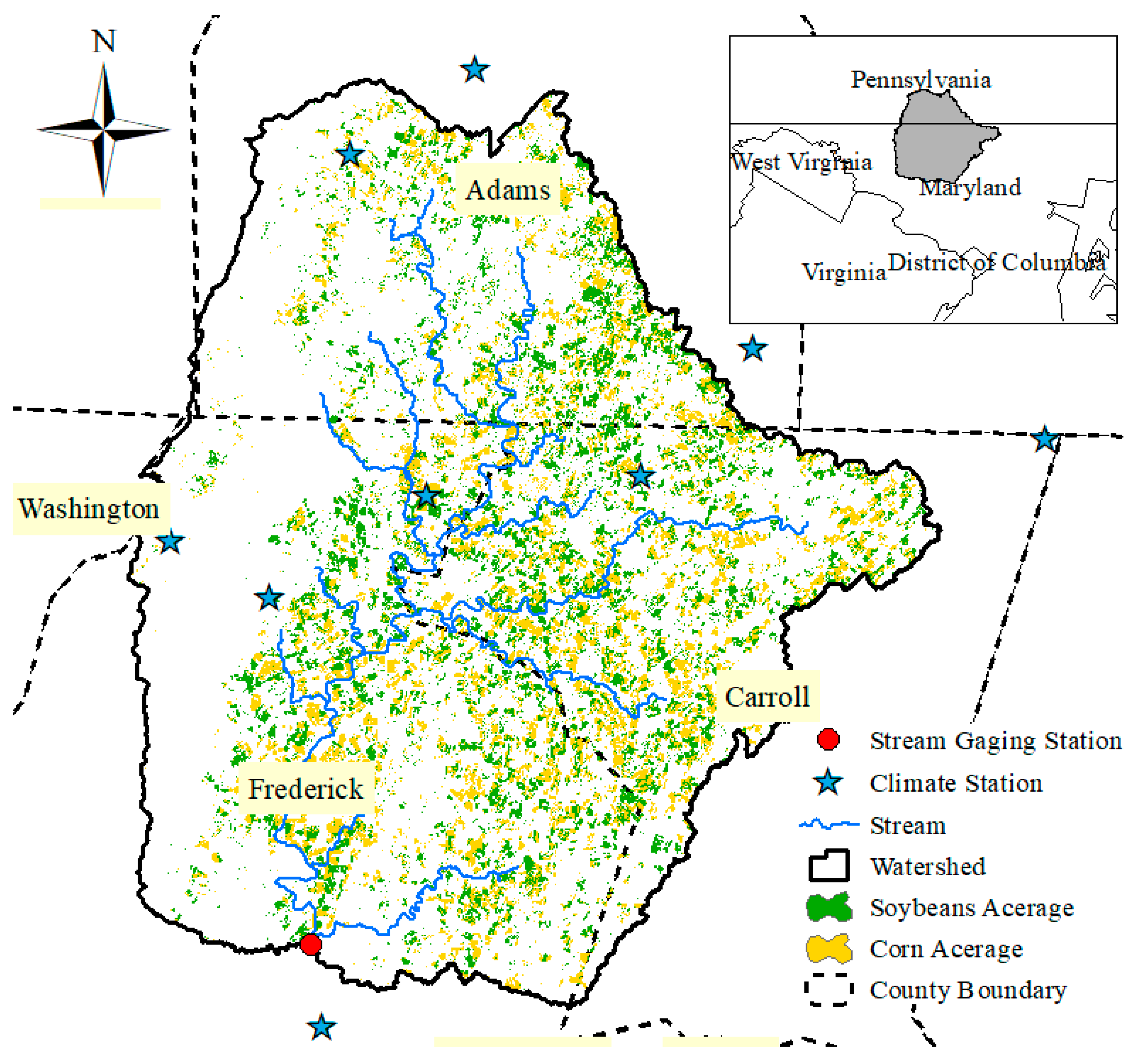
The Monocacy River Watershed (MRW) in Maryland, USA, was selected as the study area. MRW is part of the Potomac River Basin with a drainage area of approximately 2114 km2, which is located in Western Maryland bordering with south–central Pennsylvania (Figure 1). This watershed is situated within three counties of Frederick and Carroll Counties in Maryland and Adams County in Pennsylvania. According to the long–term historical data (1901–2001), average annual precipitation is about 1092.2 mm (43 in/yr), where water lost to evapotranspiration is about 711 mm (28 in/yr) or 17,000 million gallons per day (MGD) [7]. The average temperature of this region is approximately 24 °C in summer and 3 °C in winter [18]. Based on the recent climate data (2005–2014), the average annual precipitation is approximately 1135 mm, with monthly averages ranging from 72.2 to 122.1 mm. Of note is that, according to National Oceanic and Atmospheric Administration (NOAA)’s National Climatic Data Center (NOAA–NCDC), states that receive >1143 mm of annual precipitation are considered to be the wettest states within the USA [19].
The MRW is in the Western Piedmont physiographic region where the subsurface of the watershed consists of a layer of unconsolidated material or composed of soil, clay, sand, and pieces of weathered bedrock. The west side of the watershed is characterized by steep slopes consisting of highly erodible soil and the rest of the valley is mainly constituted by prime agricultural soils. According to Soil Survey Geographic (SSURGO) database, the watershed is dominated by C soil groups (47.16%), which have low infiltration rates, followed by A (29.21%) and B (23.63%) soil groups with high and moderate infiltration rates, respectively [20].
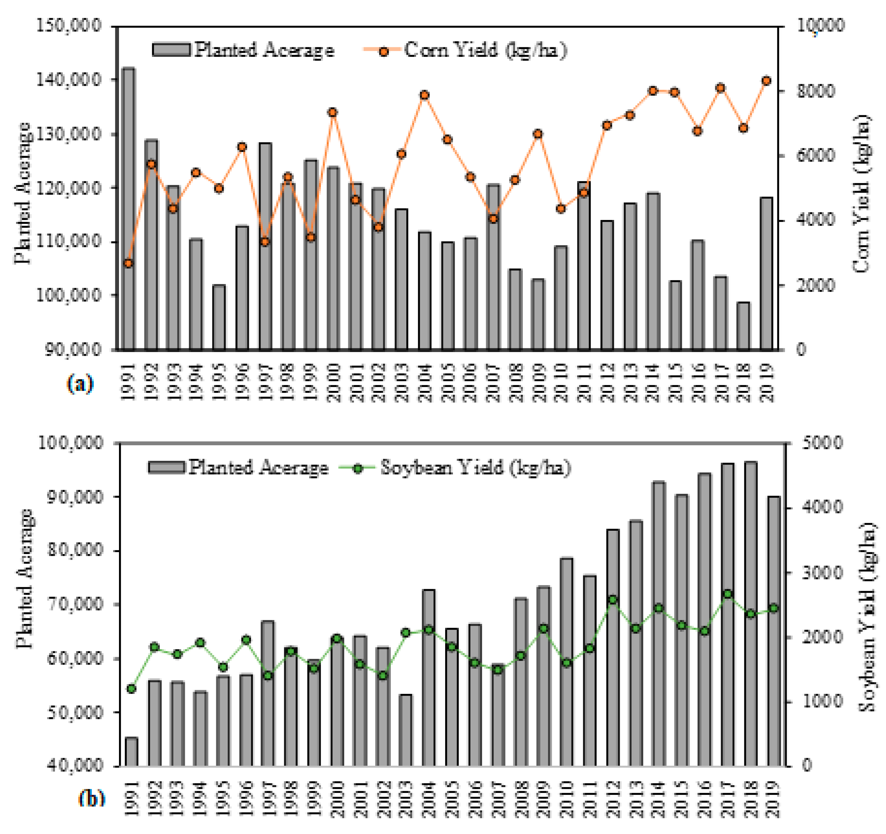
The land use and land cover of MRW is dominated by agricultural land (51.1%), followed by forests (36.2%), and urban areas (12.1%) [21]. In agricultural lands, the most dominant crops are hay (14.5%), corn (13.1%), and soybean (10.8%), respectively (Table 1). Among these crops, irrigation is mainly used for corn to maintain high yield goals [22]. Over the years, farm acreage for corn and soybean have varied. Figure 2 gives an overview of the MRW’s historical corn and soybean yield and planted acreage for the last 29 years. Despite a slight decrease in planted acreage, the corn yield has increased considerably (Figure 2). On the other hand, soybean acreage and yield have both increased in the past 29 years; however, the increasing trend for soybean production is very moderate compared to corn.
2.2. SWAT Model
The process–based models are often used for accurate simulation of the hydrological processes [23,24,25] and crop yield of the watersheds [17,25,26]. In this study, the Soil and Water Assessment Tool (SWAT) [27,28,29], was used to assess the MRW hydrology and crop yield and calculate the water productivity from the model simulations.
During the SWAT model development, the watershed is divided into a number of subbasins and each subbasin was subdivided into hydrological response units (HRUs) based on homogeneous land use, soil, and slope classes. The SWAT model computes the hydrological process and crop yield at HRU that allow for a high level of spatially detailed simulations. The SWAT model uses a water balance equation to estimate the different hydrological components (e.g., green and blue waters) at both the subbasin and HRU scales [28]. Green water includes the portion of precipitation that infiltrates and is stored in the soil as soil moisture and then returns to the atmosphere through plant transpiration and direct evaporation. Blue water includes portion of water that flows through or below the land surface and is stored in aquifer, lakes, and reservoirs. SWAT simulates the hydrologic cycle components including precipitation, evapotranspiration, surface runoff, infiltration, lateral flow, and percolation. Then, the SWAT model uses the water balance equation (Equation (1)) to update the daily soil moisture as:
where, SWt and SW0 are the soil water storage at time t and 0, respectively, Pday is the precipitation, Qsurf is the surface runoff flow, Ea is the actual evapotranspiration, wseep is the deep aquifer recharge, and Qgw is the groundwater flow. In other words, to update the daily soil moisture, the SWAT model’s hydrology component performs daily water balance by subtracting all the daily losses to surface runoff, ET, deep seepage to aquifers, and lateral groundwater flow from the daily precipitation and adds the balance to the initial soil moisture, SW0.
2.3. Model Setup
2.3.1. Model Input and Data Collection
SWAT requires elevation, land use, soil, and climate data (i.e., precipitation and temperature) to simulate the hydrological processes of the watershed. The required input data were collected as follows: Digital Elevation Model (DEM) with 30 m resolution from United States Geological Survey (USGS) National Elevation Dataset [29], land use data with 30 m resolution from the 2018 crop data layer (CDL) [21], and soil data with 250 m resolution from the SSURGO database [20]. Daily climate data, precipitation, and maximum and minimum temperature data for 19 years (2001–2019) were collected from the National Climatic Data Center (NCDC) [9]. Based on the data availability within the study time period (2001–2009), a total of 9 climate stations were selected, which are situated within close proximity of the watershed area (shown in blue star in Figure 1).
The watershed was delineated, using the watershed outlet USGS 01643000, located at the Jug bridge near Fredrick, Maryland (shown as a red point in Figure 1). Similar to climate data, the observed monthly streamflow data were collected from USGS for 19 years (2001–2019) to calibrate and validate the model. Total of 29 subbasins were delineated for MRW, and 1294 HRUs were defined with 2–5–5% thresholds for land use–soil–slope classes. The hydrological process including evapotranspiration, surface runoff, and the channel routing were computed based on the Penman–Monteith method [30], the modified Soil Conservation Service (SCS) Curve Number (CN) method [28], and the Muskingum routing methods [31], respectively. Of note is that the model outcomes were extracted using ArcGIS and figures were created in Microsoft Excel.
2.3.2. Crop Management
For this study, the two major crops, corn and soybean, were selected. In Western Maryland, planting and harvesting dates for corn depend on a number of variables and slightly change from year to year. For example, corn is generally planted at the end of April through mid–May, and soybean is planted in May. Fertilizer amount is also dependent on the soil condition and varies from field to field. However, nitrogen is applied to corn based on the targeted yield goal following the mandatory Nutrient Management Guidelines in the state of Maryland. For example, for 200 bushels/acre (13,450.22 kg/ha) of corn, around 200 lb/acre (224.17 kg/ha) of nitrogen is applied. After observing the 29 year crop yield trend, it was noticeable that crop yield varied between 65 and 175 bushels/acre and yields of more than 150 bushels/acre were observed in the last 8 years. Thus, on average, 150 lb/acre (168.13 kg/ha) nitrogen was selected as the fertilizer application rate in this study. The harvesting date was fixed after 120 days of growing days as suggested by the Maryland Cooperative Extension [22].
2.3.3. Parameter Selection and Streamflow Calibration
The calibration protocol presented by Abbaspour et al. [32] was followed to select the model parameters and calibrate the SWAT model. Based on a literature review of the existing studies on adjacent regions [33,34,35,36], in total, 17 parameters were selected for model calibration (Table 2). The initial ranges of the parameters were defined based on the suggestions from the SWAT 2012 manual [37]. The sequential uncertainty fitting (SUFI–2) algorithm on SWAT–CUP (SWAT Calibration and Uncertainty Programs) was used for the model calibration and validation process [37]. The model was calibrated for 10 years (2005–2014), with a 4-year warm–up period and was validated for another 5 years (2015–2019). For the monthly streamflow simulations, the correlation coefficient (R2), Nash–Sutcliffe coefficients (NSE), Kling–Gupta efficiency (KGE), and percent bias (PBIAS) were used as the evaluation criteria. A detailed description of these measures was described in Paul and Negahban–Azar [38]. Model performance was evaluated based on the evaluation matrix described by Moriasi et al. [39].
2.3.4. Crop Yield Calibration
After streamflow calibration and validation, the SWAT model was calibrated and validated for annual corn and soybean yields. Observed crop yields for corn and soybeans were collected for 2005–2019 from the USDA National Agricultural Statistics Service (USDA–NASS). NASS reported the grain crop yields at the county level and in bushels/acre. However, SWAT estimates the crop yield at the HRU scale and presents it in kg/ha with 20% moisture content at harvest time [25]. Thus, crop yields were converted to kg/ha following the method used in Srinivasan et al. [25]. For crop yield simulation evaluation, relative yield reduction (RYR) and root–mean–square error (RMSE) were used as the evaluation criteria. For crop yield calibration, five sensitive crop yield parameters related to harvest and leaf area were selected based on the literature review [40,41,42].
2.4. Scenarios Analysis
At first, the model was run with rainfed irrigation condition and crop yield was assessed for this scenario. Although frequent irrigation practices are evident in the Eastern Shore, according to the Maryland Department of Environment (MDE) water permit database, several groundwater wells assigned for crop irrigation are identified within this watershed in Western Maryland as well [10]. Irrigation amount, timing, and frequency are determined by the farmers based on the weather conditions, soil moisture, and growth stage. Therefore, three scenarios were developed in this study to investigate the impact of different BMPs on water productivity (WP):
Scenario 1: Model was run with the rainfed condition.
Scenario 2: Model was run with “auto irrigation” from the shallow aquifer (assigned as the main source of irrigation), which is required for each HRU. Under this scenario, an irrigation event is automatically triggered based on the defined plant–stress threshold.
Scenario 3: Model was run with updated management files considering irrigation source “outside” of the watershed. This scenario was developed considering treated wastewater reuse for irrigation purposes to match the expected high crop yield. Modified scenarios were applied for selected HRUs computing maximized irrigated areas based on the WWTP capacity.
The WP was calculated for each HRU using the SWAT simulated crop yield, and the irrigation amount was used to calculate WP (kg/m3). To understand the impact of freshwater consumption (irrigation with groundwater) and treated wastewater use on crop water productivity (WP) (kg/m3), two indices were calculated:
Here, WPIP can be defined as total crop water productivity, consisting of both rainfall and irrigation amount during the crop growth period. On the other hand, WPP can be defined as green water (rainfall) productivity, where only rainfall is consumed during the crop growth period [17]. The assumption for WPP was that, for additional irrigation water demand, freshwater withdrawal would be replaced by the treated wastewater from nearby WWTP.
3. Results and Discussion
3.1. Streamflow
SWAT model was calibrated and validated for both irrigation and rainfed management conditions, and the very minimal difference was found between these two simulations (Figure 3). Under the irrigated condition, the scores of the goodness–of–fit R2, NSE, KGE, and PBIAS for calibration periods (2005–2014) were 0.60%, 0.55%, 0.65%, and 11.1%, respectively. While under the rainfed condition, the scores of the goodness–of–fit R2, NSE, KGE, and PBIAS were 0.61%, 0.56%, 0.60%, and 10.32%, respectively. These statistics showed that the SWAT model was able to capture the observed monthly streamflow and categorized as “satisfactory” according to Moriasi et al.’s [39] performance measure and evaluation criteria. The average monthly streamflow was also well estimated during validation periods (2015–2019) with high R2, NSE, KGE, and PBIAS values of 0.85, 0.83, 0.79, and 3.92%, respectively. Thus, the high values of NSE (≥0.80) and PBIAS (<±5%) values indicate a “very good” correlation between daily observed and simulated flows, and R2 (>0.75) and KGE (≥0.75) demonstrated a “good” agreement between these. Continuous daily climate data were available after 2008 for all climate stations (showed in Figure 1). The quality of these data resulted in better model performances with higher scores of the goodness–of–fit indices during the validation period.
3.2. Crop Yield
Table 3 shows the adjustment of the parameters for crop yield calibration. Very few parameter modifications were needed to match the observed corn and soybean yields. As mentioned in Section 2.4, the model was simulated for both rainfed and irrigation managements. Table 4 shows that the model with irrigation application was able to capture both corn and soybean yields well. Thus, outcomes from this model were considered as a baseline for the analysis.
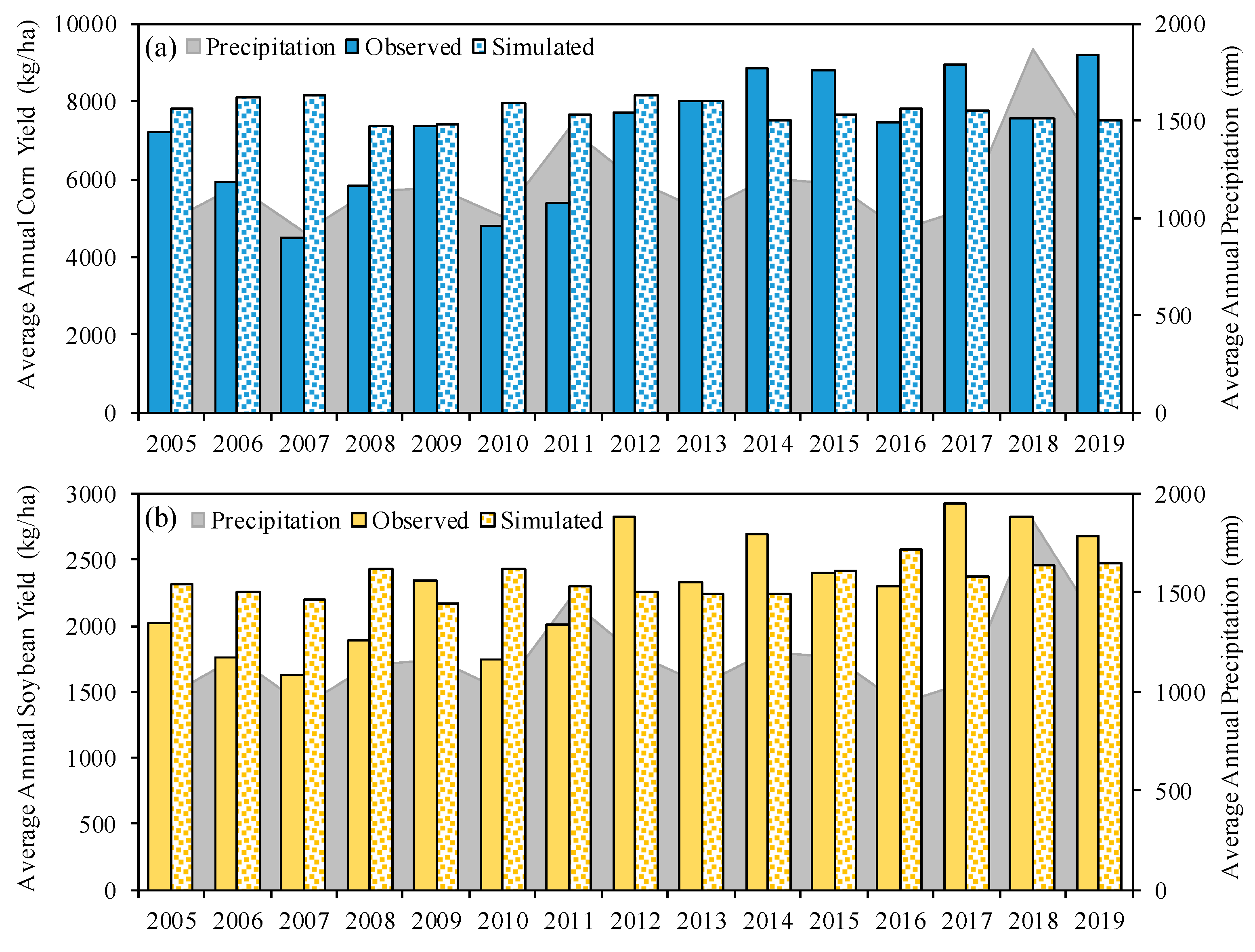
Figure 4 is showing the comparison between observed and simulated crop yields for the calibration (2005–2014) and validation (2015–2019) periods. During calibration, the simulated average crop yields for corn (7817.3 kg/ha) and soybean (2282.3 kg/ha) were higher than the observed yields of 6553.9 kg/ha and 2123.5 kg/ha, respectively. As a result, during calibration, the RMSE for corn and soybean were 1596.8 kg/ha and 373.2 kg/ha, respectively. However, the simulated corn and soybean yields during validation were closer to the observed data with a smaller RYR of 8.78% and 6.23%, respectively. RMSE was also much lower during validation than the calibration period (610.4 kg/ha and 191.3 kg/ha for corn and soybean, respectively). The RYR for corn and soybean indicates that the SWAT model overestimated (negative RYR in Table 4) the crop yield during calibration and underestimated (positive RYR in Table 4) it during the validation period. This result also indicates that over the years the fertilizer uses increases in this area. However, in this study, a fixed amount of fertilizer was used, which resulted in these RYR variations.
3.3. Irrigation Requirement
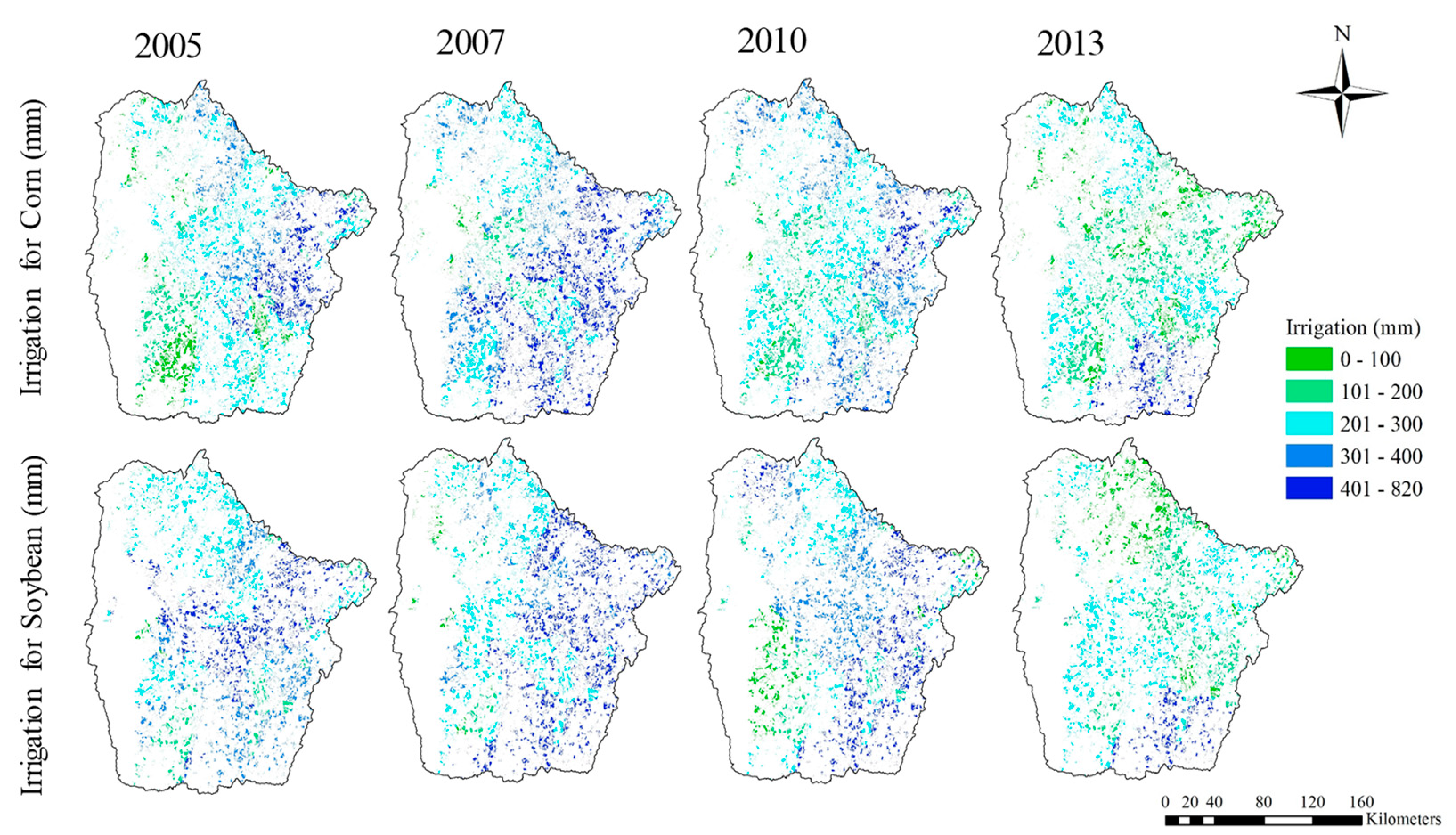
In Maryland, irrigation needs vary from year to year and depend on rainfall. Based on the SWAT model, the average irrigation for the growing season was simulated as 5.24 mm/ha (0.51 acre–ft) for corn and 6.88 mm/ha (0.65 acre–ft) for soybean. Within the simulation periods, four dry years (2005, 2007, 2010, and 2013) were selected to estimate the required irrigation demands for corn and soybean production. Figure 5 shows the applied irrigation amount for corn and soybean production at the HRU scale. The irrigation amount was varied with the HRUs and from year to year (Figure 5). However, it was noticeable that the southeastern part of the watershed required a higher amount of irrigation compared to the other regions in the study area.
It is estimated that for the high yield goal (200 bushels/acre or 13,450.22 kg/ha), 15 inches (0.38 m) of seasonal water might be needed, which would result in an annual average of 128,666 GPD (487.05 m3/day) freshwater withdrawal. It is noted that, for more than 10,000 GPD (37.85 m3/day), farmers are required to get a groundwater permit from MDE [43]. On the other hand, at least 25 acre–inches (27,154 gallons or 102.79 m3) of water is required in dry summers (zero rainfall) to maintain the expected corn production. Based on this, the simulated irrigation amount was much lower than the field application.
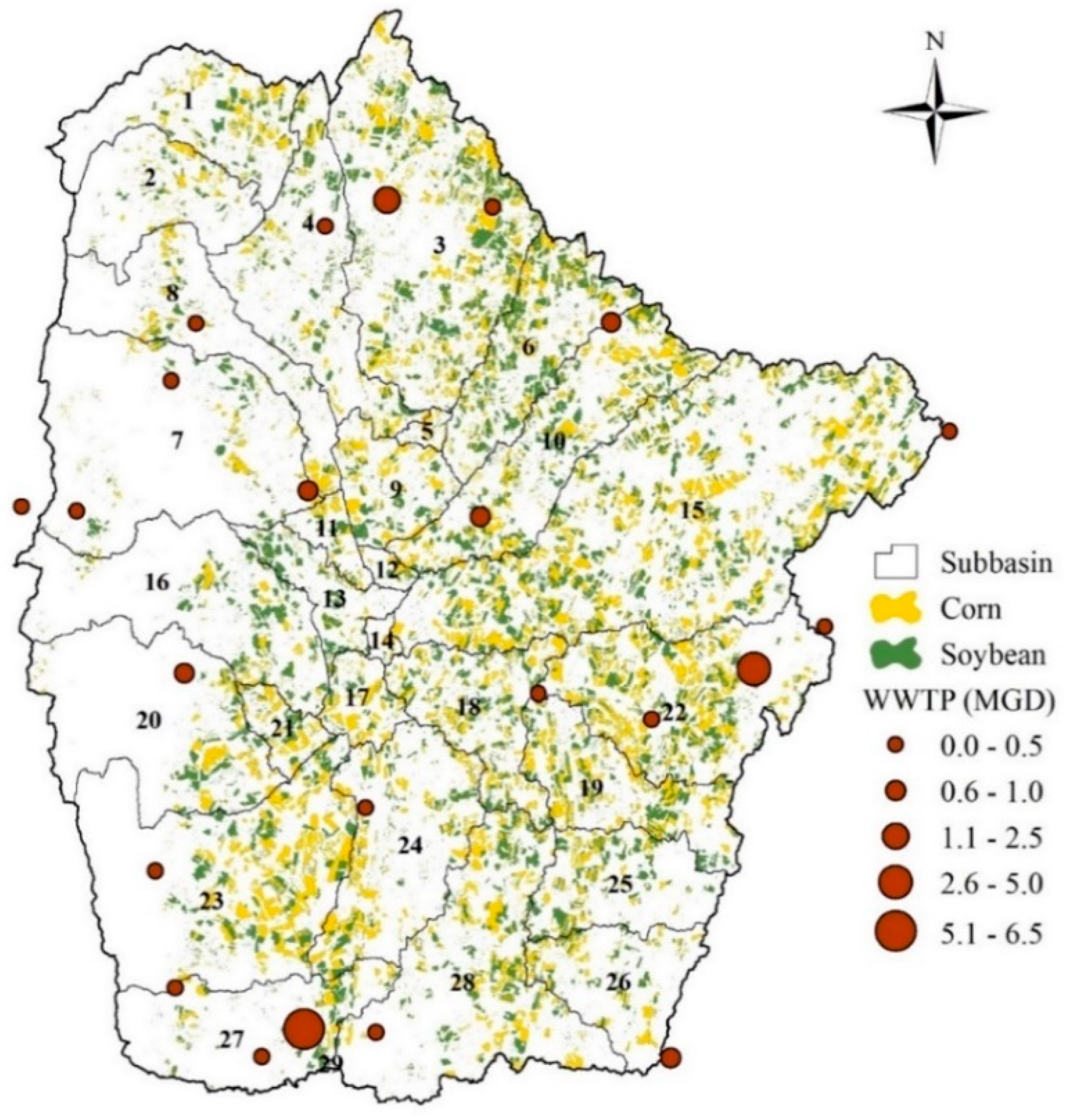
Overall, 18 publicly owned WWTPs are located within MRW, which have high water reuse potential with a discharge capacity ranging from 0.04 (0.002 m3/s) to 6.5 MGD (0.285 m3/s) (Figure 6 and Table 5). All the WWTPs are almost uniformly distributed within the watershed. Required irrigation water for 120 growing days was calculated for each crop, and the detailed estimation is presented in Table 5. Since it was difficult to identify the exact amount of irrigation for specific farmland proximities, 10 km buffer zones were created from each WWTP to locate the potential corn and soybean farmlands.
3.4. Water Productivity
Water productivity for both indices, WPIP, and WPP, were estimated based on the model–simulated crop yields and irrigation amounts. All the analysis was done at HRU levels and for the 2005–2014 period. Total water productivity (rainfall and irrigation) varied across crops. The estimated WPIP for corn was relatively higher compared to soybean. During 2005–2014, the average irrigation water productivity for corn and soybean found to be 0.617 kg/m3 and 0.173 kg/m3, respectively. Under the recycled water use scenario, the green water productivity (rainfall plus treated wastewater use) improved up to 0.713 kg/m3 for corn and 0.37 kg/m3 for soybean.
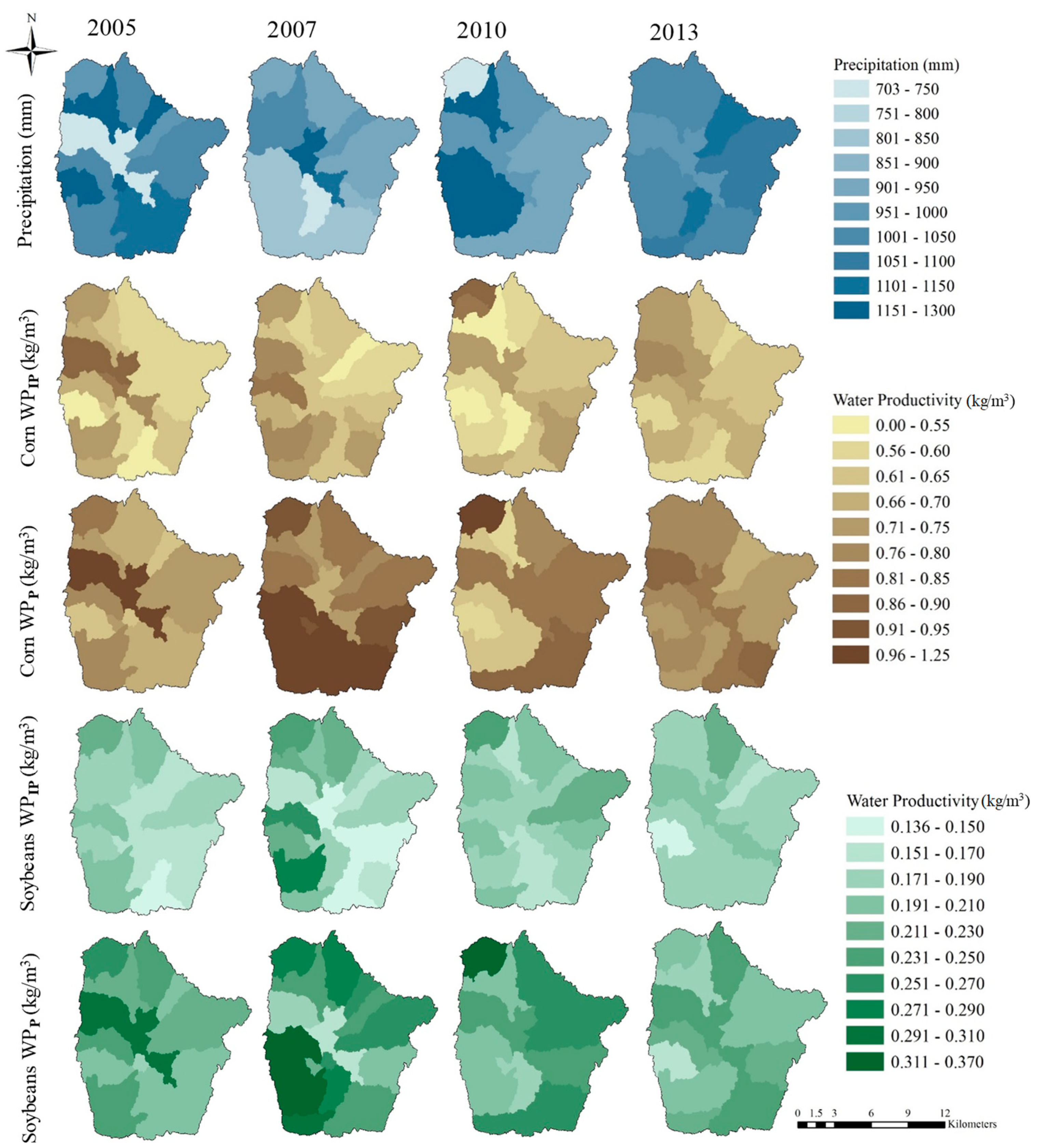
For a better understanding of irrigation use during dry years, four dry years (2005, 2007, 2010, and 2013) were selected from the total simulation period of 2005–2014. Subbasin–scale spatial variability of the corn and soybean water productivity is shown in Figure 7. From Figure 7, it is clear that the distribution of WPIP and WPP was different for each year. The water productivity of total water consumption (rainfall and irrigation) varied across crops. In the dry year (2007), the WPIP for both corn and soybean was higher on the western region of the watershed.
The green water productivity (only rainfall) also varied across crops. From Figure 7, the overall distribution of the WPP of corn and soybean was higher on those subbasins where the precipitation amount was lower. Again, higher productivity was estimated for 2007, when the average annual precipitation was much lower (906.6 mm) than in other years. For this year, the largest green water productivity for corn (>0.95 kg/m3) and soybean (>0.3 kg/m3) was found in southern subbasins where precipitation was lower than 800 mm. Thus, it was clear that instead of groundwater, the treated wastewater uses for irrigation resulted in higher WPP, especially where the rainfall amount was low.
3.5. Further Discussion
The successful implementation of sustainable water resources policies depends on long–term hydrological assessments. A DSS based on the hydrologic modeling approach was developed to investigate the “what–if” scenarios with respect to agricultural water resource management. Reclaimed wastewater from WWTPs was also considered as a potential irrigation water source in the model, and based on the simulated irrigation amount, the potentiality of treated wastewater use for irrigation was estimated considering the existing WWTP’s capacity (Section 3.3, Table 5). One of the main important aspects of reclaimed wastewater use is the economic feasibility of the project, which is mainly driven by the plant’s capacity, the cost of water, and its distribution from the source to the point of use [44,45]. Therefore, the proximity of the wastewater treatment plants to its point of use (agricultural land) and the volume of available treated wastewater are the two important decision factors to be considered in any planning. It is also acknowledged that another important decision factor is the quality of treated wastewater to minimize the human and environmental risks [44,45,46]. While assessment of treated wastewater quality was out of the scope of this study, according to MDE’s water reuse guidelines, irrigation of food crops with advanced treated wastewater (classes IV) is acceptable when there is no contact with the edible portion of the crop [47]. Thus, in this study, only publicly owned treatment works (POTW–WWTP) that treat the domestic sewages with advanced and secondary treatment processes were considered as the primary sources to obtain treated wastewater for irrigation.
In this study, it was found that the southeastern part of the study area, located in the Piedmont physiographic region, required a higher amount of irrigation compared to the other regions in the study area. This outcome confirms the previous study done by Chu and Shirmohammadi [48], where they showed that, in the Piedmont physiographic region, SWAT underestimates the subsurface flow. Furthermore, many other researchers showed that for the complicated groundwater system, the computational method used by SWAT may lead to inaccurate outcomes [48,49,50]. In addition, the variation in irrigation amounts could be also related to the different outcropping lithology, where the infiltration rate is higher (more permeable lithology), and thus, the green water available for irrigation could be lower. For future studies it is recommended to use a modified groundwater sub–model to estimate the shallow groundwater level and its interactions in the water system. Finally, it should be noted that the projected impacts of the water management BMPs on crop yields should be verified in the field. In addition, the feasibility of direct wastewater transfers across the farms should be assessed properly.
4. Conclusions
The main objective of this study was to evaluate the agricultural water use efficiency under current irrigation practices and provide water conservation strategies including the use of treated wastewater for irrigation as one of those strategies in the Mid–Atlantic agroecosystem. A quantitative method for computing the crop productivity for corn and soybean was established using a distributed hydrological model (SWAT). The results demonstrated that the SWAT model is a useful tool in calculating water productivity at the watershed scale. The water productivities for corn and soybean had spatial variabilities within the subbasins, which were mainly influenced by precipitation variability. This study also explored the treated wastewater use potentiality to increase crop water productivity and provides information for future policy implications. The overall distribution of the total and green water productivity showed that treated wastewater use for crop irrigation has a higher potential to increase water use efficiency compared to the baseline condition. During the simulation periods (2005–2014), the total water productivity (irrigation and rainfall) for corn and soybean was found to be 0.617 kg/m3 and 0.173 kg/m3, respectively, while the green water productivity (recycled water use and rainfall) was found to be 0.713 kg/m3 for corn and 0.37 kg/m3 for soybean. The highest green water productivity was estimated for the driest (<906.6 mm) year (2007) for both corn (>0.95 kg/m3) and soybean (>0.3 kg/m3), especially in the southern subbasins, where annual precipitation was lower than 800 mm. Thus, it was clear that the treated wastewater use for irrigation will result in higher WPP and reduce fresh groundwater consumption. Results from this study can be used to assess the water consumption volumes by water source and type. Another important outcome is that the SWAT model is able to calculate water productivity at both subbasin and HRU levels. This could be very useful for agricultural water managers for sustainable management of water and conservation of freshwater resources within the region and similar areas.
Author Contributions
All authors collaborated on the manuscript outline through a process facilitated by M.P. and M.N.-A. Conceptualization developed by M.P. and M.N.-A. Data acquisitions, model development, and critical analysis were done by M.P. Abstract, Section 1, Section 2 and Section 3 were drafted primarily by M.P. and M.N.-A. Review and editing were done by M.P., M.N.-A., and A.S. M.N.-A. and A.S. reviewed the manuscript including modeling results and discussion. The whole project was supervised and coordinated by M.N.-A. All authors have read and agreed to the published version of the manuscript.
Funding
This work was supported by the United States Department of Agriculture–National Institute of Food and Agriculture, Grant number 2016-68007-25064, which established CONSERVE: A Center of Excellence at the Nexus of Sustainable Water Reuse, Food, and Health.
Institutional Review Board Statement
Not applicable.
Informed Consent Statement
Not applicable.
Data Availability Statement
Not applicable.
Conflicts of Interest
The authors declare no conflict of interest.
References
- Boesch, D.F. Comprehensive Assessment of Climate Change Impacts in Maryland. In Report to the Maryland Commission on Climate Change; Maryland Department of the Environment: Baltimore, MD, USA, 2008. [Google Scholar]
- Cultice, A.K.; Bosch, D.J.; Pease, J.W.; Boyle, K.J. Horticultural producers’ willingness to adopt water recirculation technology in the Mid–Atlantic region. In Proceedings of the Agricultural & Applied Economics Association’s 2013 AAEA & CAES Joint Annual Meeting, Washington, DC, USA, 4–6 August 2013. [Google Scholar]
- NOAA–NCEI. NOAA National Centers for Environmental Information, State Climate Summaries, Maryland and District of Columbia. 2019. Available online: https://statesummaries.ncics.org/chapter/md/ (accessed on 25 January 2021).
- Luck, M.; Landis, M.; Gassert, F. Aqueduct Water Stress Projections: Decadal Projections of Water Supply and Demand Using CMIP5 GCMs; World Resources Institute: Washington, DC, USA, 2015. [Google Scholar]
- Paul, M.; Dangol, S.; Kholodovsky, V.; Sapkota, A.R.; Negahban–Azar, M.; Lansing, S. Modeling the Impacts of Climate Change on Crop Yield and Irrigation in the Monocacy River Watershed, USA. Climate 2020, 8, 139. [Google Scholar] [CrossRef]
- USGS. Water Use in the United States. 2021. Available online: https://water.usgs.gov/watuse/data/ (accessed on 25 January 2021).
- Wheeler, J.C. Freshwater–Use Trends in Maryland, 1985–2000; US Geological Survey: Places Reston, VA, USA, 2003.
- NASS. National Agricultural Statistics Service, Agricultural Statistics 2009; USDA: Washington, DC, USA, 2009.
- NOAA. Climate Data Online. 2020. Available online: https://www.ncdc.noaa.gov/cdo–web/ (accessed on 26 January 2021).
- Paul, M.; Negahban–Azar, M.; Shirmohammadi, A.; Montas, H. Developing a Multicriteria Decision Analysis Framework to Evaluate Reclaimed Wastewater Use for Agricultural Irrigation: The Case Study of Maryland. Hydrology 2021, 8, 4. [Google Scholar] [CrossRef]
- Shirmohammadi, A.M.; Rowe, S.; Kasraei, R.; Summers, B.; Michael, R.; Ortt, H.; Schmidt, R.; Shedlock, D.; Nemazi, M.; Negahban–Azar, M.; et al. Stressed Aquifers on the Coastal Plain of Maryland. In Proceedings of the American Geophysical Union (AGU), Quest for Sustainability of Heavily Stressed Aquifers at regional to Global Scales, Valencia, Spain, 21–24 October 2019. [Google Scholar]
- MDA. Agriculture in Maryland: Summary for 2010; Maryland Department of Agriculture: Annapolis, MD, USA, 2011.
- Immerzeel, W.; Gaur, A.; Zwart, S. Integrating remote sensing and a process–based hydrological model to evaluate water use and productivity in a south Indian catchment. Agric. Water Manag. 2008, 95, 11–24. [Google Scholar] [CrossRef]
- Keller, A.; Keller, J. Effective Efficiency: A water Use Concept for Allocating Fresh Water Resources and Irrigation Division Discussion Paper; Winrock International: Arlington, VA, USA, 1995. [Google Scholar]
- Garg, K.K.; Bharati, L.; Gaur, A.; George, B.; Acharya, S.; Jella, K.; Narasimhan, B. Spatial Mapping of Agricultural Water Productivity using the Swat Model in Upper Bhima Catchment, India. Irrig. Drain. 2011, 61, 60–79. [Google Scholar] [CrossRef] [Green Version]
- Han, X.; Wei, Z.; Zhang, B.; Han, C.; Song, J. Effects of Crop Planting Structure Adjustment on Water Use Efficiency in the Irrigation Area of Hei River Basin. Water 2018, 10, 1305. [Google Scholar] [CrossRef] [Green Version]
- Luan, X.; Wu, P.; Sun, S.; Wang, Y.; Gao, X. Quantitative study of the crop production water footprint using the SWAT model. Ecol. Indic. 2018, 89, 1–10. [Google Scholar] [CrossRef]
- CCBRM. Upper Monocacy River Watershed Characterization Plan. 2016. Available online: https://www.carrollcountymd.gov/media/2326/upper–monocacy–river–characterization–plan.pdf (accessed on 26 January 2021.).
- Renzulli, M. Wettest Places in the USA. 2020. Available online: https://www.tripsavvy.com/wettest–places–in–the–usa–4135027 (accessed on 29 June 2021).
- NRCS–USDA. Natural Resources Conservation Service Soils USDA. 2019. Available online: https://www.nrcs.usda.gov/wps/portal/nrcs/detail/soils/survey/?cid=nrcs142p2_053627 (accessed on 5 May 2019).
- USDA–NASS. Cropland Data Layer. National Agricultural Statistics. 2018. Available online: https://nassgeodata.gmu.edu/CropScape/ (accessed on 1 February 2021).
- Lewis, J. Estimating Irrigation Water Requirements to Optimize Crop Growth (FS–447); University of Maryland Extension: Cumberland, MD, USA, 2014. [Google Scholar]
- Narsimlu, B.; Gosain, A.K.; Chahar, B.R.; Singh, S.K.; Srivastava, P.K. SWAT Model Calibration and Uncertainty Analysis for Streamflow Prediction in the Kunwari River Basin, India, Using Sequential Uncertainty Fitting. Environ. Process. 2015, 2, 79–95. [Google Scholar] [CrossRef]
- Yesuf, H.M.; Melesse, A.M.; Zeleke, G.; Alamirew, T. Streamflow prediction uncertainty analysis and verification of SWAT model in a tropical watershed. Environ. Earth Sci. 2016, 75, 1–16. [Google Scholar] [CrossRef]
- Srinivasan, R.; Zhang, X.; Arnold, J.G. SWAT Ungauged: Hydrological Budget and Crop Yield Predictions in the Upper Mississippi River Basin. Trans. ASABE 2010, 53, 1533–1546. [Google Scholar] [CrossRef]
- Bauwe, A.; Kahle, P.; Lennartz, B. Evaluating the SWAT model to predict streamflow, nitrate loadings and crop yields in a small agricultural catchment. Adv. Geosci. 2019, 48, 1–9. [Google Scholar] [CrossRef] [Green Version]
- Arnold, J.G.; Moriasi, D.N.; Gassman, P.W.; Abbaspour, K.C.; White, M.J.; Srinivasan, R.; Santhi, C.; Harmel, R.D.; van Griensven, A.; Van Liew, M.W.; et al. SWAT: Model Use, Calibration, and Validation. Trans. ASABE 2012, 55, 1491–1508. [Google Scholar] [CrossRef]
- Neitsch, S.L.; Arnold, J.G.; Kiniry, J.R.; Williams, J.R. Soil and Water Assessment Tool Theoretical Documentation Version 2009; Texas Water Resources Institute: College Station, TX, USA, 2011. [Google Scholar]
- USGS. US Geological Survey National Map Database. Available online: http://viewer.nationalmap.gov/viewer/ (accessed on 2 July 2012).
- Monteith, J. Evaporation and environment. Symp. Soc. Exp. Biol. 1965, 19, 205–234. [Google Scholar] [PubMed]
- Arnold, J.G.; Srinivasan, R.; Muttiah, R.S.; Williams, J.R. Large Area Hydrologic Modeling and Assessment Part I: Model Development. JAWRA J. Am. Water Resour. Assoc. 1998, 34, 73–89. [Google Scholar] [CrossRef]
- Abbaspour, K.C.; Rouholahnejad, E.; Vaghefi, S.; Srinivasan, R.; Yang, H.; Kløve, B. A continental–scale hydrology and water quality model for Europe: Calibration and uncertainty of a high–resolution large–scale SWAT model. J. Hydrol. 2015, 524, 733–752. [Google Scholar] [CrossRef] [Green Version]
- Chu, T.; Shirmohammadi, A.; Montas, H.; Abbott, L.; Sadeghi, A. Watershed Level BMP Evaluation with SWAT Model. In Proceedings of the 2005 ASAE Annual Meeting, Tampa, FL, USA, 17–20 July 2005. [Google Scholar] [CrossRef]
- Sadeghi, A.M.; Yoon, K.; Graff, C.; Mccarty, G.; McConnell, L.; Shirmohammadi, A.; Hively, D.; Sefton, K. Assessing the Performance of SWAT and AnnAGNPS Models in a Coastal Plain Watershed, Choptank River, Maryland, U.S.A. In Proceedings of the ASABE Annual International Meeting, Minneapolis, MN, USA, 17–20 June 2007. Technical Papers. [Google Scholar] [CrossRef]
- Sexton, A.M.; Sadeghi, A.M.; Zhang, X.; Srinivasan, R.; Shirmohammadi, A. Using NEXRAD and Rain Gauge Precipitation Data for Hydrologic Calibration of SWAT in a Northeastern Watershed. Trans. ASABE 2010, 53, 1501–1510. [Google Scholar] [CrossRef]
- Sexton, A.M.; Shirmohammadi, A.; Sadeghi, A.M.; Montas, H.J. Impact of Parameter Uncertainty on Critical SWAT Output Simulations. Trans. ASABE 2011, 54, 461–471. [Google Scholar] [CrossRef]
- Abbaspour, K.C. Swat–Cup 2012. SWAT Calibration and Uncertainty Program—A User Manual; Swiss Federal Institute of Aquatic Science and Technology: Dübendorf, Switzerland, 2013. [Google Scholar]
- Paul, M.; Negahban–Azar, M. Sensitivity and uncertainty analysis for streamflow prediction using multiple optimization algorithms and objective functions: San Joaquin Watershed, California. Model. Earth Syst. Environ. 2018, 4, 1509–1525. [Google Scholar] [CrossRef]
- Moriasi, D.N.; Gitau, M.W.; Pai, N.; Daggupati, P. Performance measures and evaluation criteria. Trans. ASABE 2015, 58, 1763–1785. [Google Scholar]
- Lee, S.; Wallace, C.W.; Sadeghi, A.M.; Mccarty, G.W.; Zhong, H.; Yeo, I. –Y. Impacts of Global Circulation Model (GCM) bias and WXGEN on Modeling Hydrologic Variables. Water 2018, 10, 764. [Google Scholar] [CrossRef] [Green Version]
- Palazzoli, I.; Maskey, S.; Uhlenbrook, S.; Nana, E.; Bocchiola, D. Impact of prospective climate change on water resources and crop yields in the Indrawati basin, Nepal. Agric. Syst. 2015, 133, 143–157. [Google Scholar] [CrossRef]
- Uniyal, B.; Dietrich, J.; Vu, N.Q.; Jha, M.K.; Arumí, R.J.L. Simulation of regional irrigation requirement with SWAT in different agro–climatic zones driven by observed climate and two reanalysis datasets. Sci. Total Environ. 2019, 649, 846–865. [Google Scholar] [CrossRef] [PubMed]
- MDE. Maryland Department of the Environment, Water Appropriation or Use Permit. Available online: https://mde.maryland.gov/programs/permits/watermanagementpermits/pages/index.aspx (accessed on 21 May 2020).
- Bixio, D.; Thoeye, C.; Wintgens, T.; Ravazzini, A.; Miska, V.; Muston, M.; Chikurel, H.; Aharoni, A.; Joksimovic, D.; Melin, T. Water reclamation and reuse: Implementation and management issues. Desalination 2008, 218, 13–23. [Google Scholar] [CrossRef]
- Urkiaga, A.; de las Fuentes, L.; Bis, B.; Chiru, E.; Balasz, B.; Hernández, F. Development of analysis tools for social, economic and ecological effects of water reuse. Desalination 2008, 218, 81–91. [Google Scholar] [CrossRef]
- Jaramillo, M.F.; Restrepo, I. Wastewater Reuse in Agriculture: A Review about Its Limitations and Benefits. Sustainability 2017, 9, 1734. [Google Scholar] [CrossRef] [Green Version]
- MDE. Guidelines for use of Class Iv Reclaimed Water: High Potential for Human Contact. Maryland Department of the Environment; 2016. Available online: https://mde.maryland.gov/programs/Water/wwp/Documents/Water%20reuse–MDE%20Guidelines%20for%20Use%20of%20Reclaimed%20Water%20–%20Final.pdf (accessed on 5 March 2021).
- Chu, T.W.; Shirmohammadi, A. Evaluation of the Swat Model’s Hydrology Component in the Piedmont Physiographic Region of Maryland. Trans. ASAE 2004, 47, 1057–1073. [Google Scholar] [CrossRef]
- Shao, G.; Zhang, D.; Guan, Y.; Xie, Y.; Huang, F. Application of SWAT Model with a Modified Groundwater Module to the Semi–Arid Hailiutu River Catchment, Northwest China. Sustainability 2019, 11, 2031. [Google Scholar] [CrossRef] [Green Version]
- Wu, K.; Johnston, C.A. Hydrologic response to climatic variability in a Great Lakes Watershed: A case study with the SWAT model. J. Hydrol. 2007, 337, 187–199. [Google Scholar] [CrossRef]
Figure 1.
Location of Monocacy River Watershed.

Figure 2.
Historical crop yield and planted acreage for (a) corn and (b) soybean. Data collected from United States Department of Agriculture (USDA) National Agricultural Statistics Service (USDA–NASS) for 29 years (1991–2019).
Figure 2.
Historical crop yield and planted acreage for (a) corn and (b) soybean. Data collected from United States Department of Agriculture (USDA) National Agricultural Statistics Service (USDA–NASS) for 29 years (1991–2019).

Figure 3.
The hydrograph of average monthly observed and simulated discharge during (a) calibration (2005–2014) and (b) validation (2015–2019).
Figure 3.
The hydrograph of average monthly observed and simulated discharge during (a) calibration (2005–2014) and (b) validation (2015–2019).

Figure 4.
Comparison of observed (NASS) and simulated (SWAT) crop yield for corn and soybean for the (a) calibration (2005–2014) and (b) validation (2015–2019) periods.
Figure 4.
Comparison of observed (NASS) and simulated (SWAT) crop yield for corn and soybean for the (a) calibration (2005–2014) and (b) validation (2015–2019) periods.

Figure 5.
Simulated irrigation amount for corn and soybean production. Maps are presented for four dry years: 2005, 2007, 2010, and 2013.
Figure 5.
Simulated irrigation amount for corn and soybean production. Maps are presented for four dry years: 2005, 2007, 2010, and 2013.

Figure 6.
Location of WWTPs, and corn and soybean acreage within the watershed. Size of the point shows the capacity of the WWTP.
Figure 6.
Location of WWTPs, and corn and soybean acreage within the watershed. Size of the point shows the capacity of the WWTP.

Figure 7.
Spatial variability of the total (WPIP) and green water productivity (WPP) for both corn and soybean for four dry years: 2005, 2007, 2010, and 2013.
Figure 7.
Spatial variability of the total (WPIP) and green water productivity (WPP) for both corn and soybean for four dry years: 2005, 2007, 2010, and 2013.


Table 1.
Dominant crops and land use.
| Land Use and Land Cover | Area (acres) | Area (km2) | % of Watershed Area |
|---|---|---|---|
| Forest | 189,307.88 | 766.10 | 36.24 |
| Urban Area | 68,957.65 | 255.12 | 12.07 |
| Grassland | 1243.05 | 5.03 | 0.24 |
| Water | 662.31 | 2.68 | 0.13 |
| Agricultural Land | 76,200.67 | 1085.06 | 51.33 |
| Hay | 75,540.25 | 305.70 | 14.46 |
| Corn | 68,321.40 | 276.49 | 13.08 |
| Pasture | 58,279.52 | 235.85 | 11.16 |
| Soybean | 56,368.50 | 228.12 | 10.79 |
| Winter Wheat | 8315.58 | 33.65 | 1.59 |
| Alfalfa | 935.82 | 3.79 | 0.18 |
| Apple | 362.05 | 1.47 | 0.07 |
Table 2.
List of model parameters used in this study to calibrate and validate the SWAT model. The model parameter names and their definitions are listed according to SWAT input/output documentation [27].
Table 2.
List of model parameters used in this study to calibrate and validate the SWAT model. The model parameter names and their definitions are listed according to SWAT input/output documentation [27].
| Parameter | Definition | Initial Range | Calibrated Value |
|---|---|---|---|
| SOL_K | Soil saturated hydraulic conductivity (mm/h) | −25 to 25 | 10.95 |
| SOL_AWC | Available soil water capacity (mm H2O/mm soil) | −25 to 25 | 3.95 |
| ALPHA_BF | Baseflow recession constant (days) | 0.01 to 1 | 0.680 |
| GW_DELAY | Groundwater delay (days) | 1 to 500 | 113.5 |
| GW_REVAP | Groundwater “revap” coefficient | 0.01 to 0.2 | 0.011 |
| REVAPMN | Re–evaporation threshold (mm H2O) | 0.01 to 500 | 273.5 |
| GWQMN | Threshold groundwater depth for return flow (mm H2O) | 0.01 to 5000 | 115.0 |
| CN2 | Curve number for moisture condition II | −0.3 to 0.3 | 0.011 |
| EPCO | Plant uptake compensation factor | 0.01 to 1 | 0.855 |
| ESCO | Soil evaporation compensation factor | 0.01 to 1 | 0.717 |
| CH_N(2) | Main channel Manning’s n | 0.01 to 0.15 | 0.059 |
| CH_K(2) | Main channel hydraulic conductivity (mm/h) | 5 to 500 | 165.2 |
| SFTMP | Snowfall temperature (°C) | 0 to 5 | 2.1 |
| SMFMN | Melt factor for snow on 21 December (mm H2O/°C–day) | 0 to 10 | 7.1 |
| SMFMX | Melt factor for snow on 21 June (mm H2O/°C–day) | 0 to 10 | 7.3 |
| SMTMP | Snowmelt base temperature (°C) | −2 to 5 | 3.1 |
| TIMP | Snowpack temperature lag factor | 0 to 1 | 0.35 |
Table 3.
Default and adjusted crop yield parameters for corn and soybean applied at HRU scale. The model parameters name and their definitions are listed according to SWAT input–output documentation [27].
Table 3.
Default and adjusted crop yield parameters for corn and soybean applied at HRU scale. The model parameters name and their definitions are listed according to SWAT input–output documentation [27].
| Parameter | Unit | Parameter Definition | Corn | Soybean | ||
|---|---|---|---|---|---|---|
| Default | Calibrated | Default | Calibrated | |||
| BIO_E | (kg/ha)/(MJ/m2) | Radiation use efficiency or biomass energy ratio | 39 | 40 | 25 | 25 |
| HVSTI | (kg/ha)/(kg/ha) | Harvest index for optimal growing season | 0.5 | 0.5 | 0.31 | 0.3 |
| WSYF | (kg/ha)/(kg/ha) | Lower limit of harvest index | 0.3 | 0.3 | 0.01 | 0.01 |
| BLAI | (m2/m2) | Maximum potential leaf area index | 6 | 6 | 3 | 3 |
| DLAI | Fraction of growing season when leaf growth declines | 0.7 | 0.7 | 0.6 | 0.5 | |
Table 4.
Comparison of model performance for crop yield simulations between rainfed and irrigated conditions.
Table 4.
Comparison of model performance for crop yield simulations between rainfed and irrigated conditions.
| With Irrigation | Without Irrigation | ||||
|---|---|---|---|---|---|
| RYR (%) | RMSE (kg/ha) | RYR (%) | RMSE (kg/ha) | ||
| Corn | Calibration | −18.97 | 1596.8 | −24.08 | 1863.5 |
| Validation | 8.78 | 610.4 | −11.64 | 873 | |
| Soybean | Calibration | −7.48 | 373.2 | 23.81 | 501.8 |
| Validation | 6.23 | 191.3 | 32.74 | 512.2 | |
Table 5.
Estimated area of corn and soybean (in km2) where reclaimed wastewater can be applied from neighboring WWTPs. A list of existing publicly owned WWTPs is included with their capacity and discharge method information.
Table 5.
Estimated area of corn and soybean (in km2) where reclaimed wastewater can be applied from neighboring WWTPs. A list of existing publicly owned WWTPs is included with their capacity and discharge method information.
| Subbasin No. | Area (km2) | Wastewater Treatment Plant | ||
|---|---|---|---|---|
| Corn | Soybean | Flow (MGD) | Discharge Method | |
| 3 | 3.70 | 3.06 | 2.00 | Outfall to surface waters |
| 0.16 | ||||
| 4 | 1.22 | 0.93 | 0.31 | |
| 6 | 1.79 | 0.77 | 0.67 | |
| 7 | 0.19 | 0.17 | 0.06 | |
| 0.02 | ||||
| 8 | 0.43 | 0.62 | 0.18 | |
| 10 | 1.45 | 0.52 | 0.63 | |
| 11 | 1.65 | 1.17 | 0.56 | Spray irrigation |
| 18 | 0.66 | 0.36 | 0.11 | Outfall to surface waters |
| 20 | 1.03 | 0.83 | 0.91 | |
| 22 | 5.8 | 4.01 | 3.28 | |
| 0.09 | ||||
| 23 | 1.91 | 1.48 | 0.04 | |
| 0.56 | Spray irrigation | |||
| 24 | 0.24 | 0.17 | 0.08 | Outfall to surface waters |
| 26 | 0.85 | 0.63 | 0.63 | |
| 27, 29 | 4.52 | 4.71 | 6.50 | |
| 28 | 4.41 | 3.56 | 3.97 | |
Publisher’s Note: MDPI stays neutral with regard to jurisdictional claims in published maps and institutional affiliations. |
© 2021 by the authors. Licensee MDPI, Basel, Switzerland. This article is an open access article distributed under the terms and conditions of the Creative Commons Attribution (CC BY) license (https://creativecommons.org/licenses/by/4.0/).
Share and Cite
MDPI and ACS Style
Paul, M.; Negahban-Azar, M.; Shirmohammadi, A. Assessing Crop Water Productivity under Different Irrigation Scenarios in the Mid–Atlantic Region. Water 2021, 13, 1826. https://doi.org/10.3390/w13131826
AMA Style
Paul M, Negahban-Azar M, Shirmohammadi A. Assessing Crop Water Productivity under Different Irrigation Scenarios in the Mid–Atlantic Region. Water. 2021; 13(13):1826. https://doi.org/10.3390/w13131826
Chicago/Turabian StylePaul, Manashi, Masoud Negahban-Azar, and Adel Shirmohammadi. 2021. "Assessing Crop Water Productivity under Different Irrigation Scenarios in the Mid–Atlantic Region" Water 13, no. 13: 1826. https://doi.org/10.3390/w13131826
Note that from the first issue of 2016, this journal uses article numbers instead of page numbers. See further details here.