Deep Neural Network and Polynomial Chaos Expansion-Based Surrogate Models for Sensitivity and Uncertainty Propagation: An Application to a Rockfill Dam

Abstract

Computational modeling plays a significant role in the design of rockfill dams. Various constitutive soil parameters are used to design such models, which often involve high uncertainties due to the complex structure of rockfill dams comprising various zones of different soil parameters. This study performs an uncertainty analysis and a global sensitivity analysis to assess the effect of constitutive soil parameters on the behavior of a rockfill dam. A Finite Element code (Plaxis) is utilized for the structure analysis. A database of the computed displacements at inclinometers installed in the dam is generated and compared to in situ measurements. Surrogate models are significant tools for approximating the relationship between input soil parameters and displacements and thereby reducing the computational costs of parametric studies. Polynomial chaos expansion and deep neural networks are used to build surrogate models to compute the Sobol indices required to identify the impact of soil parameters on dam behavior.

1. Introduction

To meet the new challenges faced by geotechnical engineers, the use of innovative computer-based models has been growing exponentially. The complex structures and uncertainties that comprise the design of rockfill dams are a major challenge for predicting dam behavior [1,2]. Numerical methods, computational statistics and machine learning play a significant role in building improved, reliable rockfill dam models, helping to predict their behavior and reduce the cost of construction. The use of sensitivity analysis has attracted the interest of engineers seeking to understand the complex behavior associated with soil parameters. The main rationale for a sensitivity analysis using Sobol indices is to identify the most significant parameters in the variability of the output response [3]. Sensitivity analysis methods are usually categorized into local and global sensitivity analyses [4]. Local sensitivity analysis quantifies the local impact of an input parameter on a model, whereas global sensitivity analysis is focused on the uncertainty in the output due to the uncertainty in the input [5]. Numerous techniques have been developed for obtaining Sobol indices through variants of the Monte Carlo sampling technique [6] and variance-based global sensitivity analysis are performed to identify the parameters that most affect the dam stability [7], although these techniques for sensitivity analysis often require a large number of simulations [8]. The surrogate-based methods are the type more widely used, due to their efficiency and cost savings [9,10,11,12,13]. Polynomial chaos expansion based surrogate models have recently been used for the sensitivity analysis of dams [14].

This work evaluates surrogate-based and variance-based global sensitivity analyses in the design of a rockfill dam. Finite element method models (FEM) with appropriate soil parameters are often utilized for dam modeling and design [15,16,17]. Various constitutive models exist, each involving a different set of parameters, tested on and used for several geotechnical problems [18]. In this study, a two-dimensional plane–strain finite element-based model is used in Plaxis to compute the displacements and stresses for a vertical cross-section of the dam, which employs a simple constitutive soil model, the Mohr–Coulomb (MC) model [19]. The soil parameters cohesion(C), specific weight ($\rho$), shear modulus ($G_{ref}$), Poisson coefficient ($\nu$) and friction angle $\left(\varphi \right)$ are the input parameters for the MC model [20]. Moreover, the Mohr–Coulomb constitutive model is widely used in geotechnical engineering practice due to its simple nature, and fewer parameters are required as compared to other more complex constitutive models such as the Hardening Soil model (HS) [21]. The Sobol sampling method is applied to generate the samples of soil parameters as the input [22,23]. Subsequently, the parameters are assigned to the numerical model and the displacements are calculated at the positions of each of the inclinometers. Once the database of the inputs and outputs has been produced, the dam response can be estimated with respect to the uncertainty associated with the input parameters. The polynomial chaos expansion (PCE) and deep neural network (DNN) techniques [24,25,26,27] are used to build the surrogate models to evaluate the Sobol indices. The surrogate models are trained by utilizing an error function that measures the difference between the computed and measured displacements on the inclinometers.

2. Methodology

The methodology is comprised of two main phases: surrogate model approximation and sensitivity–uncertainty analysis.

2.1. Surrogate Models

In the current challenging and technically competitive environment, surrogate models can increase efficiency and reduce the computational costs of a problem or design process. Several surrogate-modeling techniques have been applied to uncertainty analysis, sensitivity analysis, and optimization. Polynomial chaos, a probabilistic approach, and deep neural networks are used in this study.

2.1.1. Polynomial Chaos Expansion (PCE)

Consider a physical model represented by a function $y=M\left(x\right)$, where $x\in {\Re }^n,y\in {\Re }^m$, and n is the number of input quantities and m the number of outputs. For simplicity, the m = 1 case will be considered in the following description. The uncertainties in the input variables and their propagation to the output lead to the description of x and y as random variables $X=(X_1,X_2,X_3,...,X_n)$ and Y, respectively [28,29,30]. For a specific value of x, the corresponding response (a realization) y is actually computed by executing a deterministic numerical solver for the non-intrusive variant of PCE. The joint probability density function (PDF) of the random vector X is denoted by ${\rho }_x$. Assuming that the input random variables $X_i$ are independent, then ${\rho }_x$ is a multiplication of the marginal probabilities, ${\rho }_x\left(X\right)={\prod }_{i=1}^n{\rho }_i\left(X_i\right)$. A polynomial Chaos Expansion approximates the response Y as a linear combination of orthonormal polynomials ${\phi }_{\alpha }\left(X\right)$:

$$\begin{array}{c}\hfill \overline{Y}\left(X\right)=\sum _{\alpha =1}^{NP}{b}_{\alpha }{\phi }_{\alpha }\left(X\right),\end{array}$$

(1)

where $b_{\alpha }$ are the expansion coefficients forming the vector $b={(b_1,b_2,b_3,...,b_{NP})}^T$. In a full PCE, the number of expansion factors $NP$ depends on the polynomial order p and the number of random input parameters n, and is given by $NP=\frac{(n+p)!}{p!n!}$. The multivariate basis of polynomials ${\phi }_{\alpha }\left(X\right)$ can be constructed as a tensor product of univariate orthonormal polynomials ${\phi }_{p_i^{\alpha }}\left(X\right)$, that is, ${\phi }_{\alpha }\left(X\right)={\prod }_{i=1}^n{\phi }_{p_i^{\alpha }}\left(X_i\right)$, where $p_i^{\alpha }$$(i=1,...,n)$ is a multi-index vector. The optimal choice of the univariate polynomial basis function is closely related to the probability density functions ${\rho }_i\left(X_i\right)$ [29]. For instance, Legendre polynomials serve as an optimal basis function for uniform distributions. The polynomial chaos expansion coefficients $b_{\alpha }$ can be computed in a non-intrusive and affordable way using a regression approach. A dataset D is composed of N input vectors $X_D={(x_D^{\left(1\right)},x_D^{\left(2\right)},...,x_D^{\left(N\right)})}^T$ sampled from the PDF ${\rho }_x$, and their corresponding responses are put in a vector $Y_D={(y_D^{\left(1\right)},y_D^{\left(2\right)},...,y_D^{\left(N\right)})}^T$, with $y_D^{\left(i\right)}=M\left(x_D^{\left(i\right)}\right)$. The expansion coefficients with a regularization term can be obtained by minimizing the error ${\sum }_{i=1}^N{(y_D^{\left(i\right)}-\overline{Y}\left(x_D^{\left(i\right)}\right))}^2+{\lambda }_P{b}^{T}b$. Defining $\Phi$ as the design matrix whose components are ${\phi }_j\left(x_D^{\left(i\right)}\right)(i=1,...,N;j=1,...,NP)$, the expansion coefficients vector is then given as the solution of the ordinary least-squares system:

$$\begin{array}{c}\hfill b={({\mathsf{\Phi }}^T\mathsf{\Phi }+{\lambda }_{P}I)}^{-1}{\mathsf{\Phi }}^T{Y}_D,\end{array}$$

(2)

where ${\lambda }_P$ is a regularization parameter and I is the identity matrix. The number of sample points is defined as $N=\gamma$$NP$, and $\gamma \ge 1$ is an oversampling parameter used to control the accuracy of the PCE [31,32]. The sample input vectors can be generated using efficient sampling algorithms such as the Latin hypercube sampling algorithm (LHS) or the Sobol scheme [22,23,33]. Once the expansion coefficients are computed, the polynomial expansion defined in Equation (1) can be used to predict the approximate response for any input variable (within the learning domain). For instance, the mean and the variance of the response can be computed using the basis function orthonormality property [32]. Their expressions are given by:

$$\begin{array}{c}\hfill {\mu }_D=\int \overline{Y}{\rho }_{x}dX=\int \left(\sum _{\alpha =1}^{NP}{b}_{\alpha }{\phi }_{\alpha }\left(X\right)\right){\rho }_{x}dX=b_1,\end{array}$$

(3)

and

$$\begin{array}{c}\hfill {\sigma }_D^2=\int {(\overline{Y}-{\mu }_D)}^2{\rho }_{x}dX=\sum _{\alpha =2}^{NP}{b}_{\alpha }^2.\end{array}$$

(4)

Remark 1.

The input variables are assumed to be independent in the above approach. However, it is possible to use the Rosenblatt transformation [34] to formulate the problem as a function of auxiliary independent variables.

2.1.2. Deep Neural Networks

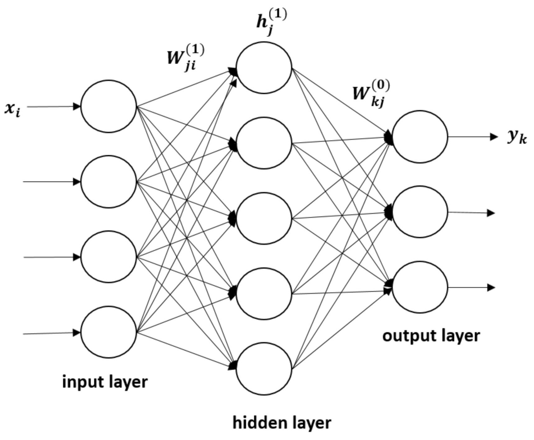
Deep neural networks (DNN) are widely considered to be a powerful and general numerical approach to building a nonlinear mapping between a set of inputs (features) and their corresponding outputs (labels or targets). Deep neural networks are well known in data science, with various applications in science and engineering. In the PCE approach, the surrogate model is comprised of linear combinations of fixed basis functions. Such models have useful practical applications, but they may be limited by the curse of dimensionality for large datasets. It should be mentioned that much effort has been invested in reducing the severity of the curse of dimensionality by using sparse expansions [35]. Furthermore, in order to apply such models to large-scale problems, the basis functions must be adapted to the data. There is a large body of literature on deep networks [25,26,27], and a brief description is given next. Deep neural networks use parametric forms for basis functions, in which parameter values are adapted during training. Moreover, with respect to these parameters, the model is nonlinear as it uses nonlinear activation functions. Figure 1 illustrates a DNN with one hidden layer. The input data are mapped to the hidden layer (1) to compute

$$\begin{array}{c}\hfill h_j^{\left(1\right)}=f(\sum _{i=1}^n{W}_{ji}^{\left(1\right)}{x}_i+a_j^{\left(1\right)}),\end{array}$$

(5)

which are then fed to the output layer $\left(o\right)$ to compute the response

$$\begin{array}{c}\hfill y_k=g(\sum _{j=1}{W}_{kj}^{\left(0\right)}{h}_j^{\left(1\right)}+a_k^{\left(0\right)}),\end{array}$$

(6)

where f and g are activation functions, $W_{ji}^{\left(1\right)},W_{kj}^{\left(0\right)}$ are the weight parameters and $a_j^{\left(1\right)},a_k^{\left(0\right)}$ are the bias parameters.

The number of neurons in the input layer is the number of input features n, and m is the dimension of the neural network response vector $Y_{NN}$. The number of hidden layers in a deep neural network and the number of neurons in each hidden layer are hyperparameters, which are optimized by experimentation guided by monitoring validation and test errors. To determine the weights and bias parameters, the network is trained on the dataset by minimizing the loss (error) function. As described earlier, a dataset D is composed of N input vectors $X_D={(x_D^{\left(1\right)},x_D^{\left(2\right)},...,x_D^{\left(N\right)})}^T$, which are sampled from the PDF, and of the corresponding targets, which are put in a vector $Y_D={(y_D^{\left(1\right)},y_D^{\left(2\right)},...,y_D^{\left(N\right)})}^T$ with $y_D^{\left(i\right)}=M\left(x_D^{\left(i\right)}\right)$. In regression problems, the mean square error (MSE), also called the loss function, between the model outputs and the labels (targets), is used along with a regularization term:

$$\begin{array}{c}\hfill J=\frac{1}{N}\sum _{i=1}^N\left\{\frac{1}{2}\sum _{k=1}^m{\left[y_k^{\left(i\right)}-y_{D,k}^{\left(i\right)}\right]}^2\right\}+\lambda \sum _{l,\alpha ,\beta }{\left(W_{\alpha \beta }^{\left(l\right)}\right)}^2,\end{array}$$

(7)

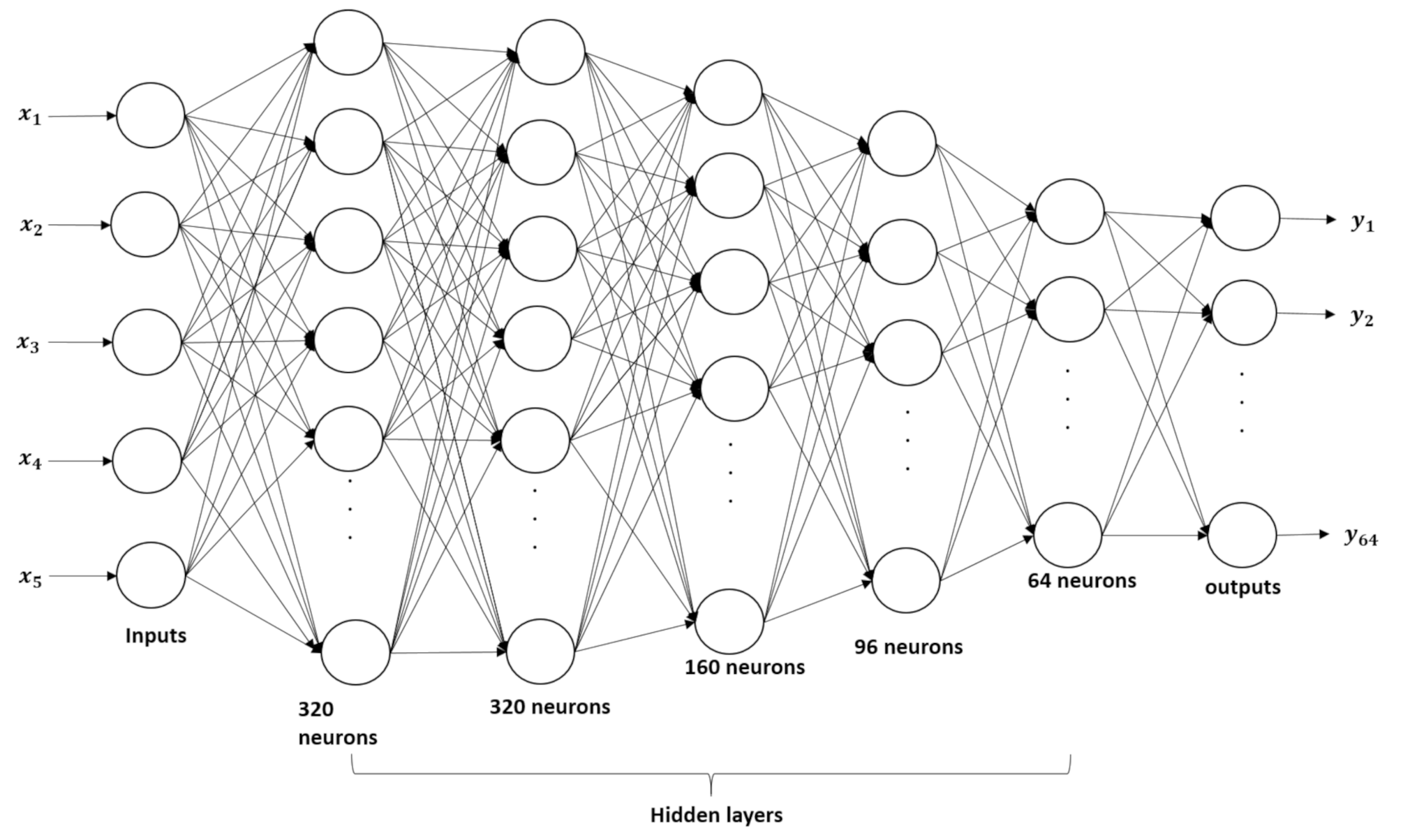
where $\lambda$ is a regularization hyperparameter. An iterative approach based on the back-propagation algorithm is used to minimize the loss function. The activation function f is usually the sigmoid or the rectified linear unit, while g is the identity function for our regression problem. An example of a deep network is presented in Figure 2, where five hidden layers are used; the input layer has $n=5$ input parameters, and the output layer has $m=64$ responses $(Y_{NN}={(y_1,y_2,...,y_{64})}^T)$.

It can be shown that minimizing the error function $E_D$ in Equation (8) is equivalent to minimizing the negative log of the likelihood function, under an assumed Gaussian distribution noise in the targets, with an assumed constant variance ${\sigma }_D^2$.

$$\begin{array}{c}\hfill E_D=\frac{1}{N}\sum _{i=1}^N\left\{\frac{1}{2}\sum _{k=1}^m{\left[y_k^{\left(i\right)}-y_{D,k}^{\left(i\right)}\right]}^2\right\}=\frac{1}{2N}\sum _{i=1}^N{(Y_D-Y_{NN})}^2.\end{array}$$

(8)

Moreover, maximizing the log-likelihood with respect to the noise variance gives the solution ${\sigma }_{D,ML}^2=\frac{1}{N}{\sum }_{i=1}^N{(Y_D-Y_{NN})}^2$. Therefore, the prediction of the network for a given input parameter vector X is given by a Gaussian probability distribution with a mean $\overline{Y}\left(X\right)=Y_{NN}$ and a variance ${\sigma }_{D,ML}^2$, which represents the noise in the data. There are many public domain implementations of (standard) deep neural networks, such as the TensorFlow library [36]. In this work, the Matlab deep learning neural toolbox is used [37].

2.1.3. Ensemble of Models

In machine learning, ensembling is a technique used to improve the predictive performance and reduce the generalization error by training several models separately and subsequently combining their solutions [24,25,26,27]. The idea here is that the ensemble (i.e., averaged solution) will perform at least as well as any of its members. Given a dataset, different neural network solutions can be obtained by varying the numbers of layers, the number of neurons for each layer, the training algorithm, the hyperparameters, and so forth. A simple and efficient approach is to use several random initializations of the weights. This option has proven to be efficient enough to generate an ensemble with partially independent members [38]. Given a mixture of K trained neural networks, each member outputs a solution with a mean $Y_{NN}^{\left(k\right)}$ and a variance ${\sigma }_{D,ML}^{\left(k\right)}$, an averaged single normal mean distribution can be defined with a mean $\overline{Y}\left(X\right)=Y_{NN}^{ens}$, where:

$$\begin{array}{c}\hfill Y_{NN}^{ens}=\frac{1}{K}\sum _{k=1}^K{Y}_{NN}^{\left(k\right)}\end{array}$$

(9)

and a variance given by:

$$\begin{array}{c}\hfill {\sigma }_{ens}^2=\frac{1}{K}\sum _{k=1}^K\left\{({\sigma }_{D,ML}^{\left(k\right)}{)}^2+{\left(Y_{NN}^{\left(k\right)}\right)}^2\right\}-{\left(Y_{NN}^{ens}\right)}^2.\end{array}$$

(10)

K is typically taken between five and 12 (in the following numerical results, it is assumed to be equal to ten). Therefore, the numerical prediction of the network is represented by a Gaussian with the mean $\overline{Y}\left(X\right)$ and the variance ${\sigma }_{ens}^2$, which represents uncertainties in both the data and in the weights.

2.2. Global Sensitivity Analysis

Sensitivity analysis provides a means of determining the effects of variations of input parameters on the outputs of a model. If a small change in input parameters results in a relatively significant difference in the output, then the parameter is considered significant for the model. In a global sensitivity analysis, all the inputs are varied simultaneously over their range, and are usually considered independent. The fundamental steps constituting the global sensitivity analysis technique are: (i) specification of the computational model; (ii) determination of relevant inputs and their bounds; (iii) input sample generation by a sampling design method; (iv) evaluation utilizing the generated input parameters; and (v) uncertainty analysis and calculation of the relative importance of each input through a sensitivity estimator. For more mathematical details, see [39] and references therein. The code described in [39] is also used for the present case study.

3. Case Study: Application to Romaine-2 Dam

A real rockfill dam was selected for a case study in order to illustrate the application of the surrogate modeling methodology for a global sensitivity analysis and an uncertainty analysis. Figure 3a illustrates a 2D cross-section of the Romaine-2 dam built in Quebec (Canada) [40,41]. The dam is 112 m high, and has an asphalt core and is grouted on a rock foundation. The asphalt core is surrounded by crushed stones having a maximum size of 80 mm, which act as supports. The transition zone $\left(N\right)$ lies next to the support region $\left(M\right)$, composed of crushed stones having a maximum size of 200 mm. Moreover, the particles with a maximum size of 600 mm are used in the inner shell zone $\left(O\right)$ and in the outer region $\left(P\right)$, composed of rocks with a maximum size of 1200 mm. Two vertical inclinometers named INV1 and INV2 are installed at two different positions (see Figure 3a) to measure the vertical displacements, considered the measured data in this study. Using the plane strain hypothesis, a finite element of the dam structure was built using the commercial code Plaxis [42]. A mesh of $\left(2187\right)$ triangular elements with 15 nodes each is presented in Figure 3b, where the different soil sub-domains are meshed accordingly, and more refinement is used around the asphalt core. A mesh convergence study [43] showed that the mesh is fine enough. To simplify the study, the Mohr–Coulomb $\left(MC\right)$ constitutive law was used, given that the dam was heavily compacted during construction [40]. Indeed, a detailed numerical study [43] showed that the discrepancies between the MC results and those obtained with the more sophisticated Hardening Soil model [21] for this rockfill dam are not significant. A dataset D was built using Sobol’s sampling algorithm to generate N sets of $n=5$ physical parameters related to the sub-domain (P). The parameters include the cohesion (C), specific weight ($\rho$), shear modulus ($G_{ref}$), Poisson coefficient ($\nu$) and the friction angle $\left(\varphi \right)$. For a sample $\left(i\right)$, the input vector is then $x_D^{\left(i\right)}={(C^{\left(i\right)},{\rho }^{\left(i\right)},G_{ref}^{\left(i\right)},{\nu }^{\left(i\right)},{\varphi }^{\left(i\right)})}^T$. The parameters are supposed to follow a uniform distribution. Several types of distributions could be utilized if more data are available to generate the sample set of soil parameters. The dilatancy angle is set relative to the friction angle as $\psi =\varphi -30$ (in degrees). Only the parameter variations in zone $\left(P\right)$ are considered in this study, as this domain covers the maximum portion of the dam. Ideally, all sub-domain parameters could be included, but for the sake of illustration, only zone $\left(P\right)$ is considered, as it is the most significant. The displacement fields corresponding to N sets of inputs $x_D^{\left(i\right)}$ are obtained by running Plaxis [42]. The displacements on a number of points (32 in this case) on each inclinometer are extracted, yielding a response vector $Y_D^{\left(i\right)}$ of dimension $m=64$.

Table 1. Soil parameter values or intervals of variations for zones P, N, O and M.

Soil Parameters	Units	P		N	O	M
		Lower Bound	Upper Bound
Cohesion $\left(C\right)$	KNm${}^{-2}$	0	${10}^{-3}$	0	0	0
Specific weights $\left(\rho \right)$	KNm${}^{-3}$	21.375	23.625	23.7	22.5	24.5
Shear modulus $\left(G_{r}ef\right)$	KNm${}^{-2}$	25,000	35,000	64,000	45,000	110,000
Poisson coefficient $\left(\nu \right)$	$--$	0.234	0.3465	0.33	0.22	0.33
Friction angle $\left(\varphi \right)$	degree	40.85	45.15	47	45	47

presents the parameter interval of variations of zone P and the parameter values of zones N, O and M. The parameter estimates in Table 1 are based on a previous study conducted in [40,43].

3.1. Sample Size Convergence Study

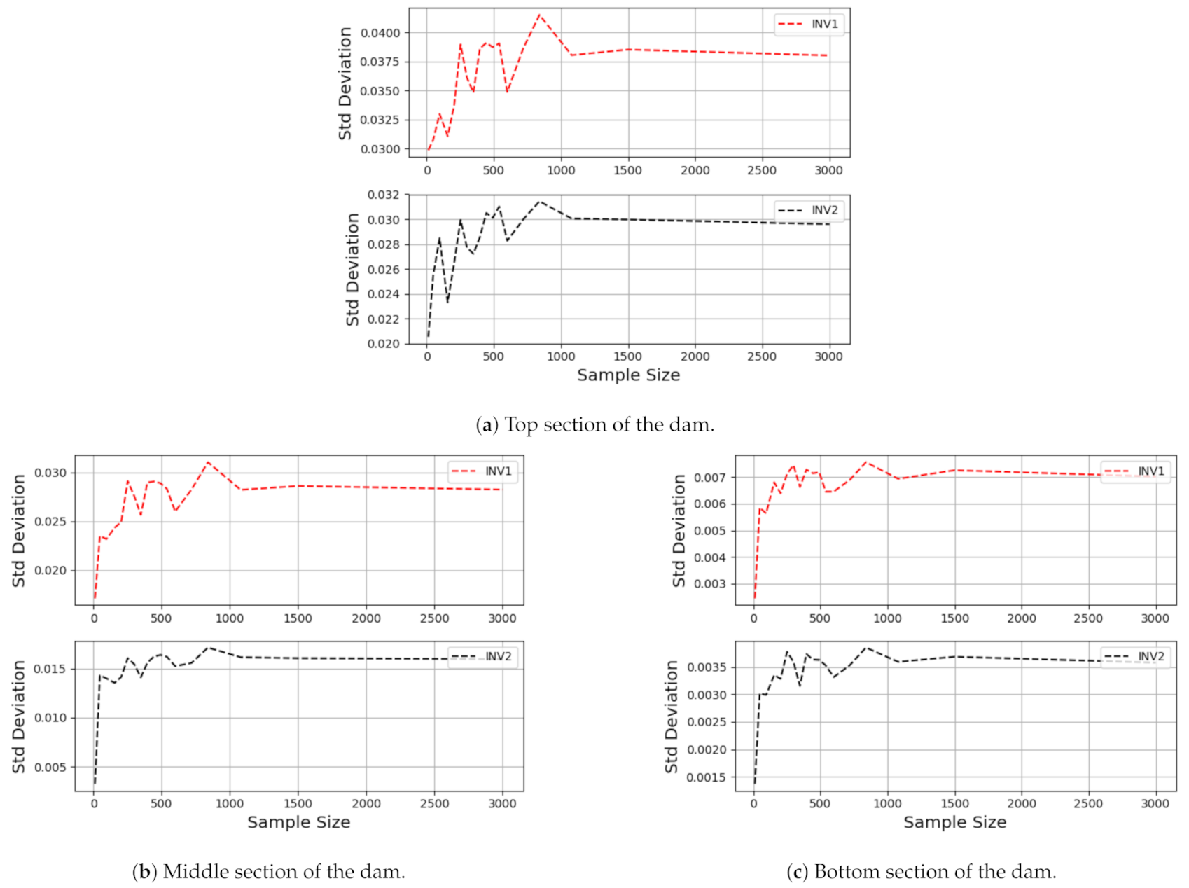
The Sobol sampling technique [44] was used to generate the samples by varying their size N $(N=12,48,96,156,204,252,300,348,392,444,496,512$, $600,720,840,900,1080,1500$ and $3000)$. The corresponding numerical simulations were performed using Plaxis, which required 587 CPU hours on an Intel-i7 PC, for N $=3000$. To build confidence in the generated database, a convergence study with respect to N was performed for the standard deviation of the vertical displacement at the 64 measurement points on the inclinometers. To check the convergence for this statistical study, standard deviation plots were built for the sample size at three positions on each inclinometer: at the top, middle and bottom (see Figure 4). The standard deviations show some fluctuations as the sample size is increased up to 1080; however, between sample sizes 1080 and 3000, the standard deviation is close to constant (up to $1\%$ of variation), which implies that sample size 1080 is sufficient for subsequent sensitivity studies.

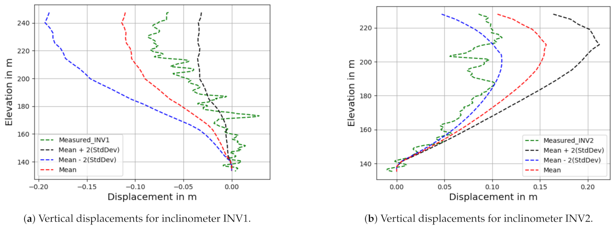
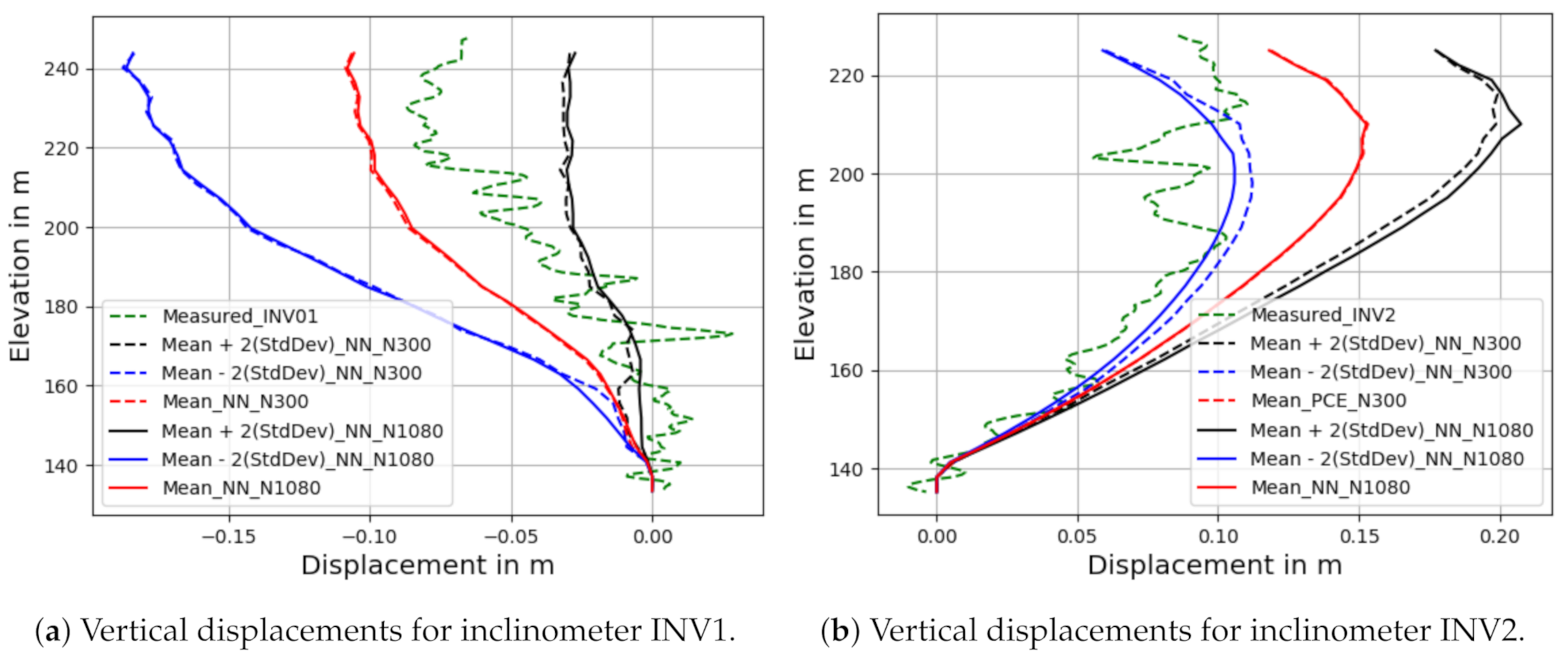
The confidence intervals for the displacements (mean $\pm 2$ standard deviation) obtained by using this classical statistical analysis (which is in fact a Monte Carlo simulation (MCS)) are shown in Figure 5. The measured data for each inclinometer are also represented in this figure, revealing fluctuations that can be attributed to some external effects such as the installation process, calibrations, temperature variations and human factors, which may have influenced some probes in the inclinometers. At the bottom, where the displacements should be zero, there is instead a $2.5$ cm displacement. Therefore, the uncertainty in the measured displacement is estimated to be at least $\pm 2.5$ cm. Figure 5 shows that, considering the uncertainties, the measured data are mostly within the predicted numerical confidence intervals, especially when the displacements are more significant. The statistical confidence intervals could be enlarged by changing the distribution intervals of the input parameters. Indeed, we used a priori uniform distributions on estimated input intervals [40].

3.2. Sobol Indices

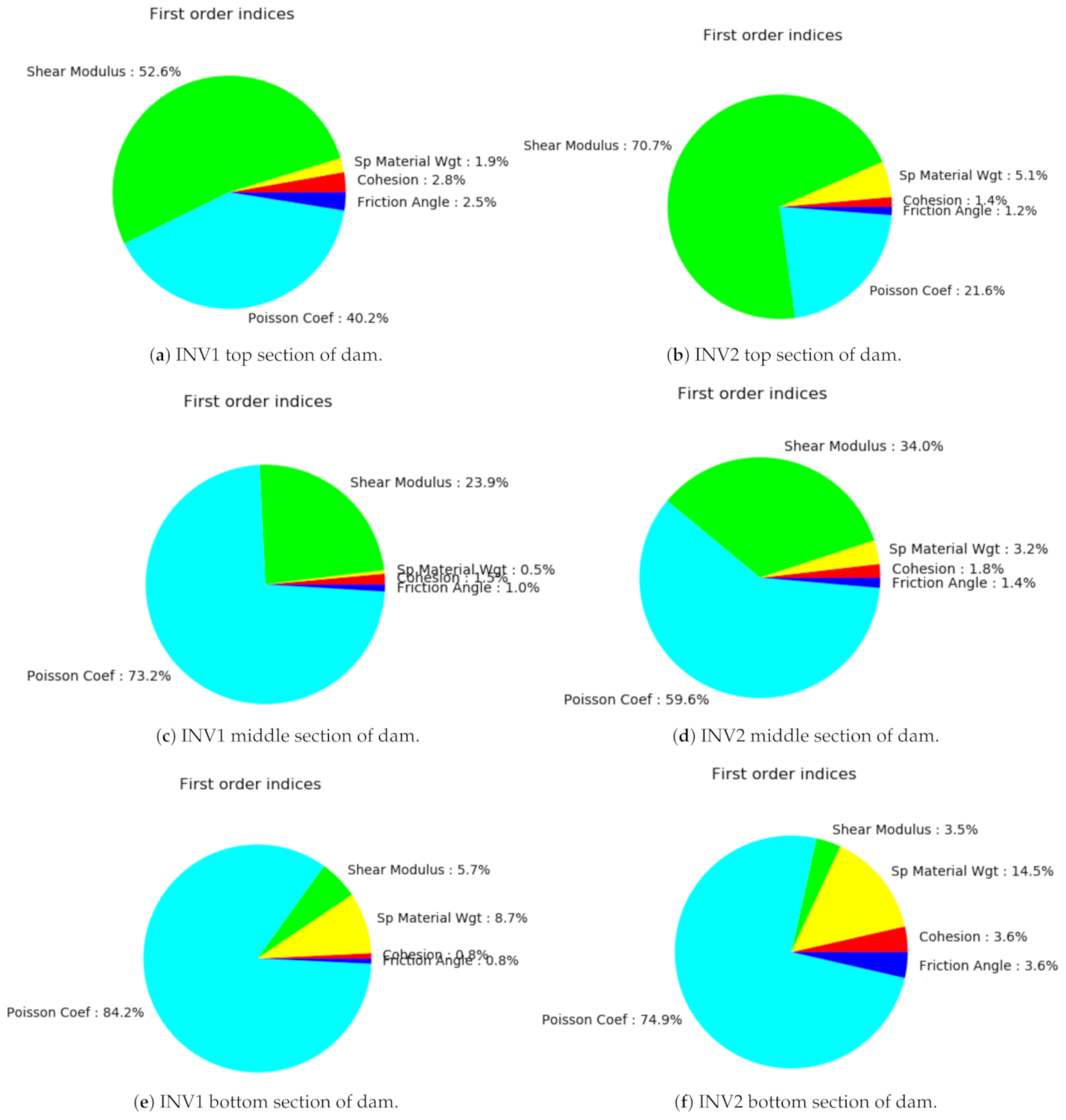
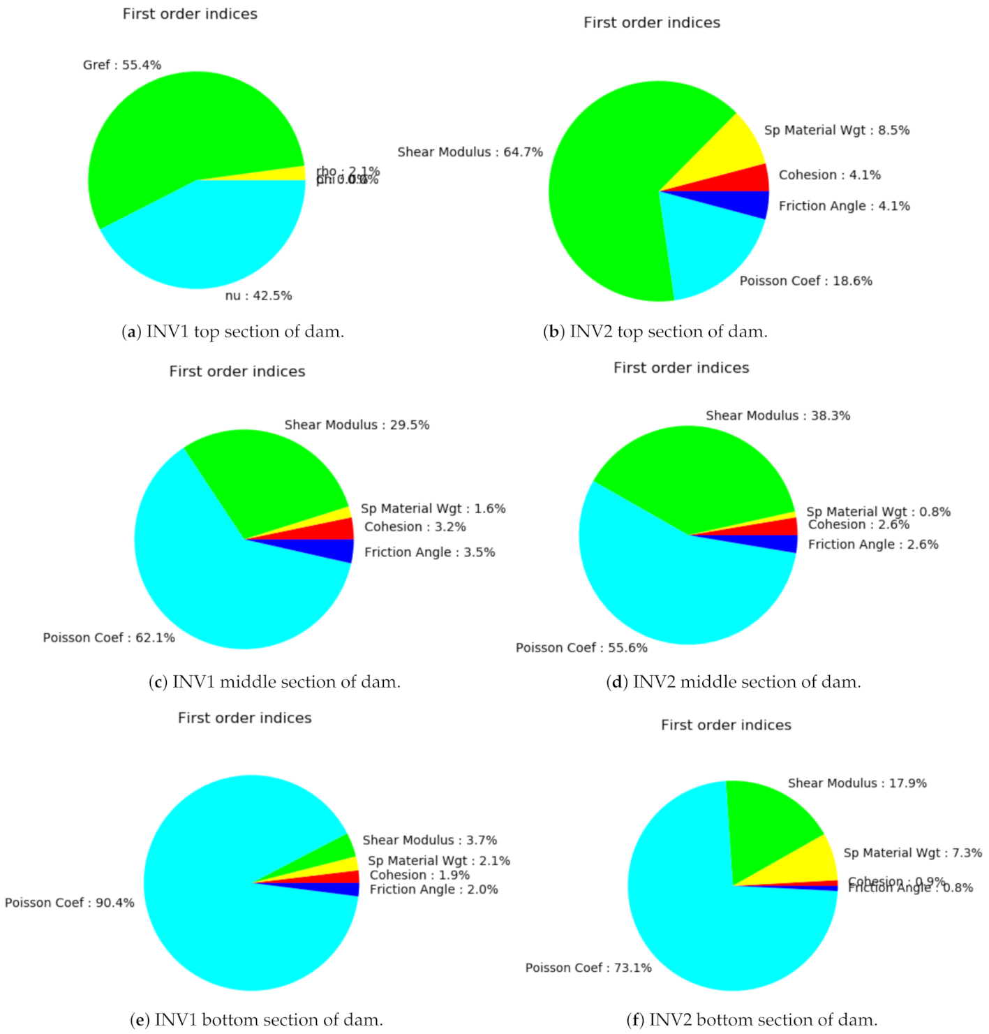
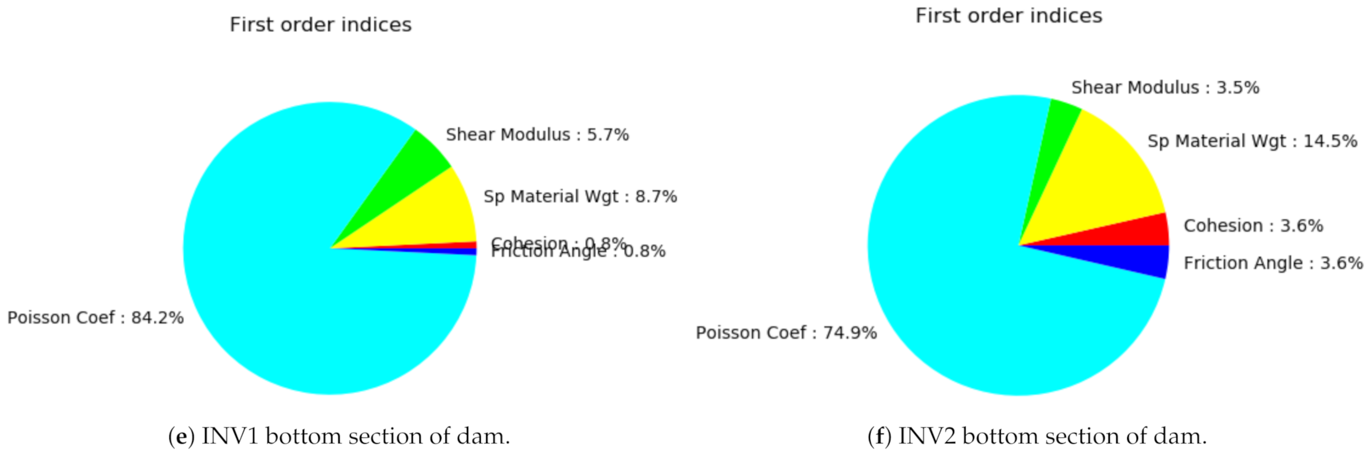
A Sobol index is defined as the ratio of partial variances to the total variance, and reflects the relative importance of each input parameter [45], as shown in Figure 6 for points located at the top, middle and bottom of the inclinometers. The indices here range from 0 to 1. It is evident from Figure 6 that the shear modulus is the dominant parameter, with a contribution of $44\%$ to $71\%$ in the top sections of the dam, and that it diminishes gradually with the depth. The Poisson’s coefficient is the second most significant parameter, with a smaller effect $(24\%)$ on top, and a high impact $(84\%)$ close to the foundation. At 140 m is the foundation (made up of routed rocks) of the dam, therefore the impact of soil parameters is abrupt at the bottom.

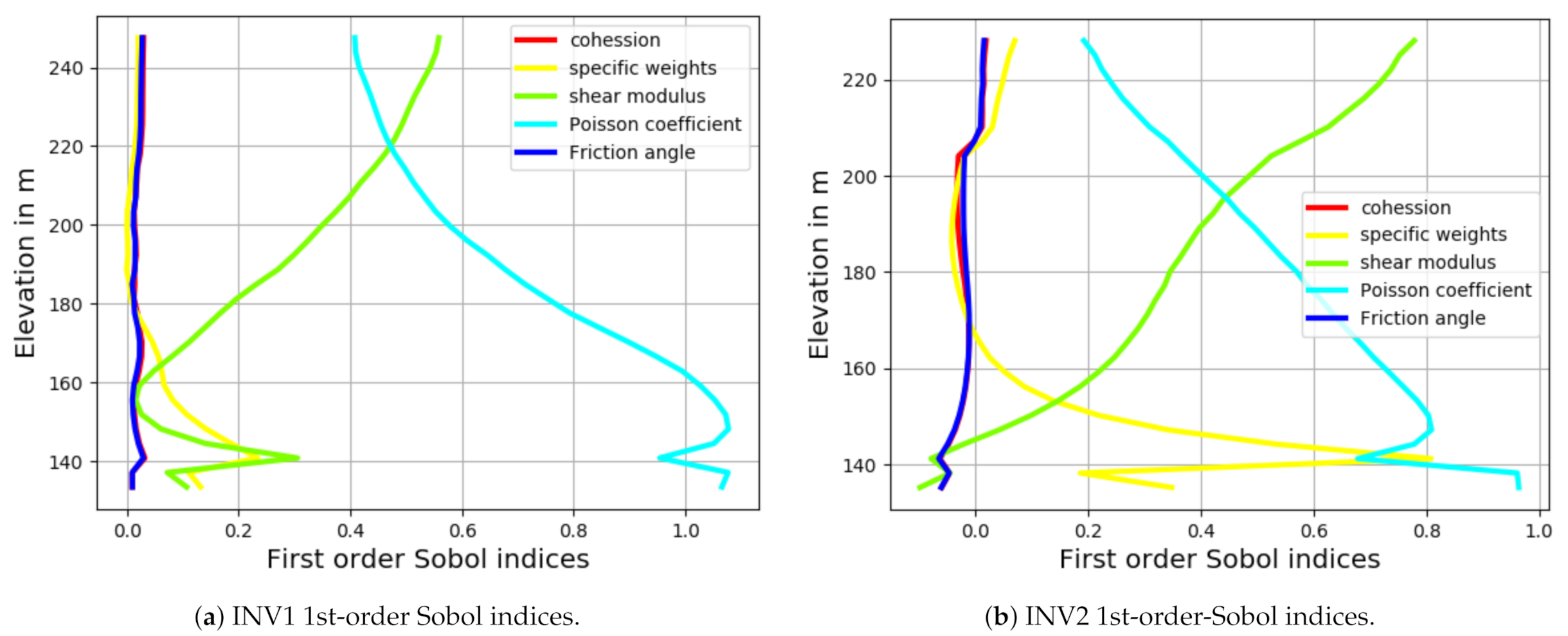
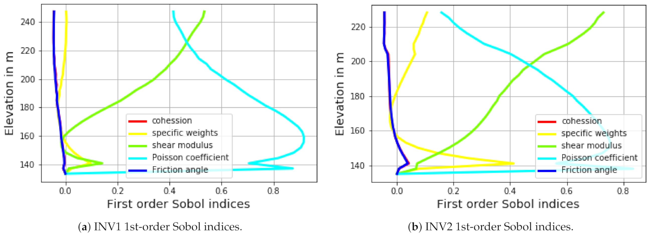
The first-order indices are calculated along the inclinometers, as shown in Figure 7. As stated earlier, for both inclinometers, the shear modulus is dominant in the upper section of the dam. The Poisson’s coefficient is another crucial parameter influencing the dam’s behavior. While it is less influential at the top section, its impact increases as we head towards the bottom part. The specific weight only affects the lower section; thus, the shear modulus and Poisson coefficients are the most significant parameters, although their contributions vary with the elevation.

3.3. Surrogate Modeling

Surrogate modeling is an approach aimed at generating an approximate numerical model to reduce the computing time, especially when a large number of simulations are required, as is the case in uncertainty and sensitivity analysis. Instead of using the ‘full-order’ original finite element model, an approximate one called a ‘surrogate model’ (or surface response) is built using the input–output database. Many techniques could be used, but here we consider polynomial chaos expansions and deep neural networks. Based on the convergence study in Section 3.1, the $N=1080$ datasets is accurate enough to build the surrogate models. To assess the accuracy of these models, we examine the residual errors (the root mean square error (RMSE) and the coefficient of determination $\left(R^2\right)$).

3.3.1. Polynomial Chaos Expansion (PCE)

A polynomial chaos expansion-based method [46] is a probabilistic technique that can be used to build an accurate surrogate model. The degree of the polynomials and the regularization parameters are tuned to get the best results. The PCE degree is varied from 2 to 6, and the regularization parameter ${\lambda }_P$ is taken as $0.001$, $0.01$ and $0.1$, respectively.

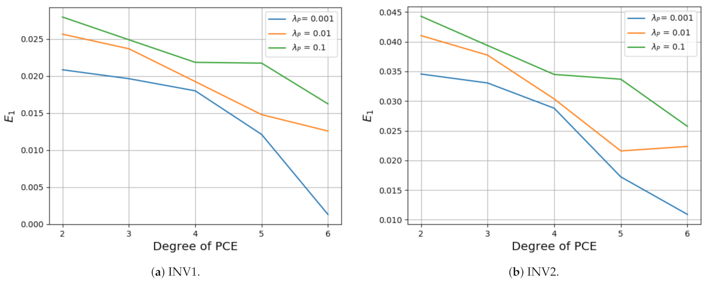
The mean and standard deviation are calculated using the surrogate model obtained by running a simple Monte Carlo method on the PCE. The evaluation of the absolute mean error with respect to the polynomial order and the regularization parameter for an output response is shown in Figure 8, and is defined as:

$$\begin{array}{c}\hfill E_1=\frac{1}{m}\sum _{i=1}^m\parallel Y_{mp}^i-Y_{ms}^i\parallel ,\end{array}$$

(11)

where m is the number of nodes and $Y_{mp}$ denotes the mean of predicted displacement at the same node as $Y_{ms}$, the simulated displacements. Ideally, ${\lambda }_P$ is selected as the smallest value which avoids overfitting. Figure 8 shows that, for $0.001$, 0.01 and $0.1$, the value $E_1$ decreases with the polynomial degree for both inclinometers. Therefore, the results for $P=6$ and ${\lambda }_P=0.001$ are considered the most reliable.

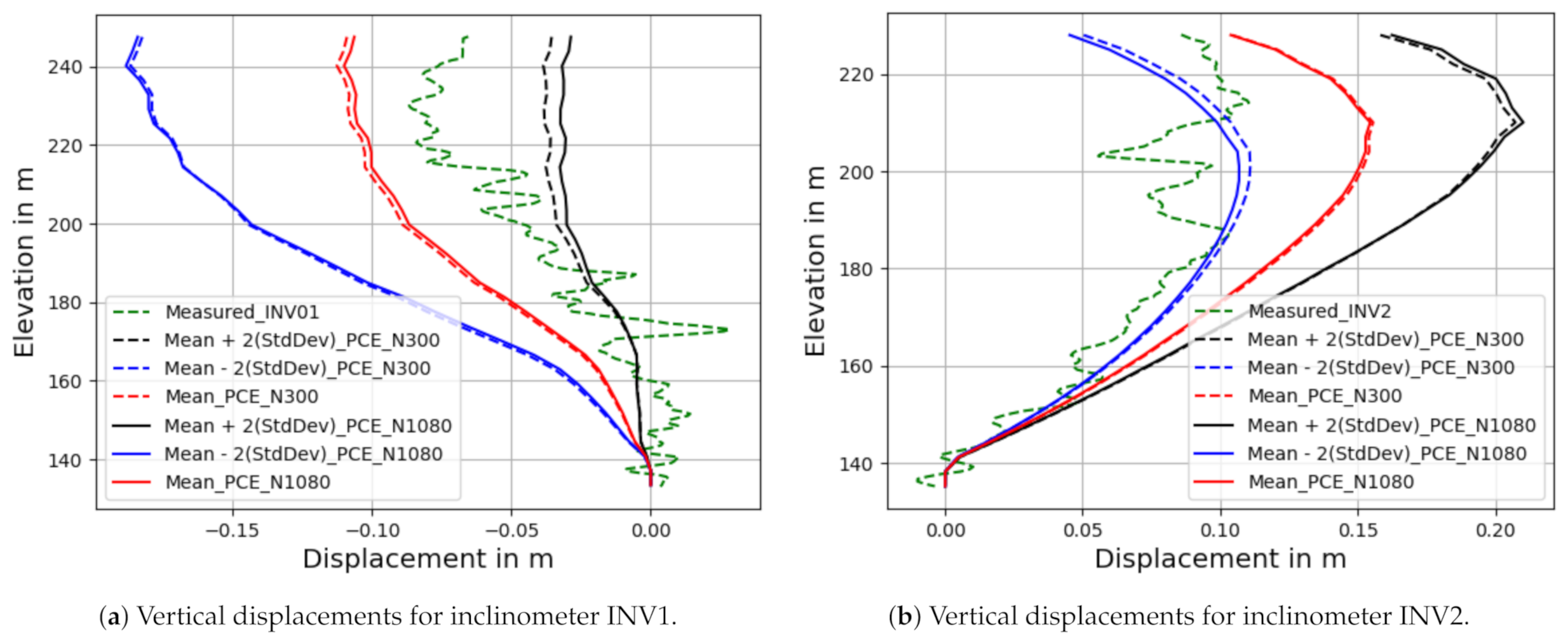
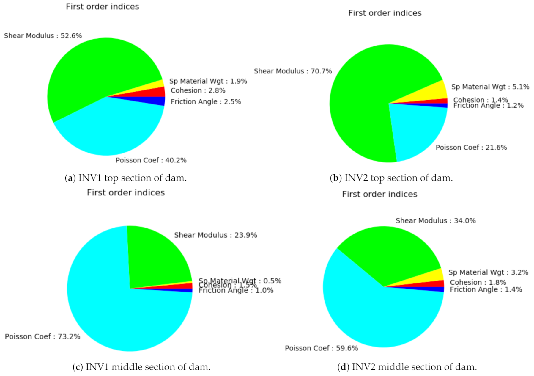
Figure 9 shows that the measured and predicted displacements obtained using PCE trained for datasets N = 300 and N = 1080 are in good agreement. Moreover, when considering the measurements along with their uncertainties, we see that they are mostly within the predicted numerical confidence intervals of PCE, especially when the displacements are more significant. The first-order indices along the inclinometers by using PCE are shown in Figure 10. As stated earlier, for both inclinometers, the shear modulus is dominant in the upper section of the dam. The Poisson’s coefficient is another crucial parameter influencing the dam’s behavior. While it is less influential at the top section, its impact increases as we head towards the bottom part. The specific weight only affects the lower section. Thus, the shear modulus and Poisson coefficients are the most significant parameters, although their contributions vary with the elevation. The Sobol indices at the top, middle and bottom of the dam are also recomputed based on the PCE surrogate model, as shown in Figure 10 and Figure 11, which illustrates almost the same information and conclusions as those shown in Figure 6 and Figure 7.

The shear modulus is the dominant parameter, with a contribution of $50\%$ to $70\%$ in the top sections of the dam, and whose influence diminishes gradually with the depth. The Poisson coefficient is the second most significant parameter, with a smaller effect ($18\%$) on top and a high impact ($90\%$) close to the foundation.

3.3.2. Deep Neural Network Results

In order to fit the data, a MATLAB function ‘Neural Net Fitting’ is used with a five-layer feedforward network, as shown in Figure 2. A scaled conjugate gradient algorithm was used for the training. The ($N=1080$ and $N=300$) datasets were divided into training, validation and testing subsets, in the following proportions: $70\%$, $15\%$, and $15\%$ respectively. An ensemble of ten trained networks was created by randomly initializing the weights in the training, and the outputs were predicted individually and averaged to obtain an ensemble output solution. An example of plots for datasets N = 300 and N = 1080, showing the fitness variation with respect to the training iterations (epochs), is presented in Figure 12.

The mean and standard deviation are calculated using the surrogate model obtained by running a simple Monte Carlo method on the ensemble neural network model. The mean and variance for the ensemble model are computed by Equations (9) and (10).

The displacements obtained with the ensemble neural network are shown in Figure 13, and are very similar to those obtained with the statistical approach in Figure 5, and are represented in the pie charts and the indices as shown in Figure 14 and Figure 15, respectively. The displacement standard deviations are calculated on the inclinometers using the statistical approach (MCS) and the PCE surrogate models and DNN models are reported in

Table 2. Comparative study of standard deviation in m by numerical simulations and surrogate models for top, middle and bottom sections of the dam.

Inclinometers	INV1			INV2
Approach	Top	Middle	Bottom	Top	Middle	Bottom
Statistical approach (MCS)	0.0388	0.0282	0.0043	0.0292	0.0161	0.0028
Polynomial Chaos Expansion (PCE)	0.0364	0.0291	0.0084	0.0313	0.0238	0.0079
Ensemble of Deep neural networks	0.0387	0.0311	0.00121	0.0285	0.0189	0.0042

, with a maximum standard deviation for all methods close to 4 centimeters. Moreover, near the foundation of the dam the displacements are almost zero.

Figure 16 shows the computational efficiency for the cpu for one Plaxis realization and for the surrogate models with respect to the number of samples for the soil parameters. It can be observed that the surrogate models are more efficient at predicting the results as compared to obtaining the simulations with the FEM model. It is worth noting that this result will be helpful for an upcoming study that consists of the identification of soil parameters by inverse analysis. In the inverse analysis, the optimization algorithm makes hundreds of calls to obtain the numerical solutions [47]. Therefore, the surrogate models will be used instead of the full-order original finite element model for computational efficiency. The outcome of this study is that, indeed, NN requires many fewer samples to realize a sensitivity or identification analysis compared to the full-order model.

4. Conclusions

This paper contributes to the sensitivity and uncertainty analysis for rockfill dams using the surrogate modeling approach. The approach was applied to a real rockfill dam with an asphalt core. Two surrogate models were developed, namely, a polynomial chaos expansion (PCE) model and a deep neural network (DNN) by training two datasets N = 300 and N = 1080. Their results were compared to those obtained with Monte Carlo simulations. The variance-based sensitivity analysis reinforces the fact that the shear modulus and the Poisson coefficient are the parameters that play the most significant role in the dam’s behavior. Therefore, when considering all material sub-domains, these two parameters may be kept as the only significant uncertain parameters, thereby significantly reducing the total number of uncertain inputs. A second analysis was conducted by sampling the input parameters using a uniform probability distribution. Overall, this study shows that building surrogate models reduces the computational cost of numerical models when a large number of simulations is required, as in sensitivity and uncertainty analyses.

References

- Bowles, L. Foundation Analysis and Design; McGraw-Hill: New York, NY, USA, 1996. [Google Scholar]
- Calvello, M.; Finno, R.J. Selecting parameters to optimize in model calibration by inverse analysis. Comput. Geotech. 2004, 31, 410–424. [Google Scholar] [CrossRef]
- Homma, T.; Saltelli, A. Importance measures in global sensitivity analysis of nonlinear models. Reliab. Eng. Syst. Saf. 1996, 52, 1–17. [Google Scholar] [CrossRef]
- Saltelli, A.; Ratto, M.; Andres, T.; Campolongo, F.; Cariboni, J.; Gatelli, D.; Saisana, M.; Tarantola, S. Global Sensitivity Analysis: The Primer; John Wiley & Sons: Hoboken, NJ, USA, 2008. [Google Scholar]
- Cacuci, D.G.; Ionescu-Bujor, M.; Navon, I.M. Sensitivity and Uncertainty Analysis, Volume II: Applications to Large-Scale Systems; CRC Press: New York, NY, USA, 2005; Volume 2. [Google Scholar]
- Dimov, I.; Georgieva, R. Monte carlo algorithms for evaluating sobol’sensitivity indices. Math. Comput. Simul. 2021, 81, 506–514. [Google Scholar] [CrossRef]
- Segura, R.L.; Miquel, B.; Paultre, P.; Padgett, J.E. Accounting for uncertainties in the safety assessment of concrete gravity dams: A probabilistic approach with sample optimization. Water 2021, 13, 855. [Google Scholar] [CrossRef]
- Branbo, R.S.; Hassan, I. Seepage sensitivity analysis through a homogeneous dam within the unsaturated soil zone. J. Eng. And Computer Sci. JECS 2020, 21, 64–74. [Google Scholar]
- Huang, C.; Radi, B.; Hami, A.E. Uncertainty analysis of deep drawing using surrogate model based probabilistic method. Int. J. Adv. Manuf. Technol. 2016, 86, 3229–3240. [Google Scholar] [CrossRef]
- Guo, X.; Dias, D. Kriging based reliability and sensitivity analysis: Application to the stability of an earth dam. Comput. Geotech. 2020, 120, 103411. [Google Scholar] [CrossRef]
- Sargsyan, K. Surrogate Models for Uncertainty Propagation and Sensitivity Analysis, Handbook of Uncertainty Quantification; Ghanem, R., Higdon, D., Owhadi, H., Eds.; Springer: New York, NY, USA, 2017. [Google Scholar]
- Stephens, D.; Gorissen, D.; Crombecq, K.; Dhaene, T. Surrogate based sensitivity analysis of process equipment. Appl. Math. Model. 2011, 35, 1676–1687. [Google Scholar] [CrossRef] [Green Version]
- Forrester, A.; Sobester, A.; Keane, A. Engineering Design via Surrogate Modelling: A Practical Guide; John Wiley & Sons: Hoboken, NJ, USA, 2008. [Google Scholar]
- Hariri-Ardebili, M.A.; Mahdavi, G.; Abdollahi, A.; Amini, A. An rf-pce hybrid surrogate model for sensitivity analysis of dams. Water 2021, 13, 302. [Google Scholar] [CrossRef]
- Duncan, J.M. State of the art: Limit equilibrium and finite-element analysis of slopes. J. Geotech. Eng. 1996, 122, 577–596. [Google Scholar] [CrossRef]
- Owen, D.; Hinton, E. Finite Elements in Plasticity; Technical Report; Pineridge Press Limited: Swansea, UK, 1980. [Google Scholar]
- Pietruszczak, S. Fundamentals of Plasticity in Geomechanics; CRC Press: Boca Raton, FL, USA, 2010. [Google Scholar]
- Pramthawee, P.; Jongpradist, P.; Kongkitkul, W. Evaluation of hardening soil model on numerical simulation of behaviors of high rockfill dams. Songklanakarin J. Sci. Technol. 2011, 33, 325–334. [Google Scholar]
- Wood, D.M. Soil Behaviour and Critical State Soil Mechanics; Cambridge University Press: Melbourne, Australia, 1990. [Google Scholar]
- Labuz, J.F.; Zang, A. Mohr–coulomb failure criterion. In The ISRM Suggested Methods for Rock Characterization, Testing and Monitoring: 2007–2014; Springer: New York, NY, USA, 2012; pp. 227–231. [Google Scholar]
- Schanz, T.; Vermeer, P.; Bonnier, P. The Hardening Soil Model: Formulation and Verification, Beyond 2000 in Computational Geotechnics; A.A. Balkema: Avereest, The Netherlands, 1999; pp. 281–296. [Google Scholar]
- Dige, N.; Diwekar, U. Efficient sampling algorithm for large-scale optimization under uncertainty problems. Comput. Chem. Eng. 2018, 115, 431–454. [Google Scholar] [CrossRef]
- Burhenne, S.; Jacob, D.; Henze, G.P. Sampling based on sobol’sequences for monte carlo techniques applied to building simulations. In Proceedings of the Building Simulation 2011: 12th Conference of International Building Performance Simulation Association, Sydney, Australia, 14–16 November 2011; pp. 1816–1823. [Google Scholar]
- Breiman, L. Bagging predictors. Mach. Learn. 1996, 24, 123–140. [Google Scholar] [CrossRef] [Green Version]
- Goodfellow, I.; Bengio, Y.; Courville, A. Deep Learning; MIT Press: Cambridge, MA, USA, 2016. [Google Scholar]
- Bishop, C.M. Pattern Recognition and Machine Learning; Springer: New York, NY, USA, 2006. [Google Scholar]
- Hsieh, W.W. Machine Learning Methods in the Environmental Sciences: Neural Networks and Kernels; Cambridge University Press: New York, NY, USA, 2009. [Google Scholar]
- Blatman, G.; Sudret, B. An adaptive algorithm to build up sparse polynomial chaos expansions for stochastic finite element analysis. Probabilistic Eng. Mech. 2010, 25, 183–197. [Google Scholar] [CrossRef]
- Xiu, D.; Karniadakis, G.E. The wiener–askey polynomial chaos for stochastic differential equations. SIAM J. Sci. Comput. 2002, 24, 619–644. [Google Scholar] [CrossRef]
- Hariri-Ardebili, M.A.; Sudret, B. Polynomial chaos expansion for uncertainty quantification of dam engineering problems. Eng. Struct. 2020, 203, 109631. [Google Scholar] [CrossRef]
- Hosder, S.; Walters, R.; Balch, M. Efficient sampling for non-intrusive polynomial chaos applications with multiple uncertain input variables. In Proceedings of the 48th AIAA/ASME/ASCE/AHS/ASC Structures, Structural Dynamics, and Materials Conference, Honolulu, HI, USA, 23–26 April 2007; p. 1939. [Google Scholar]
- Abdedou, A.; Soulaimani, A. A non-intrusive b-splines bézier elements-based method for uncertainty propagation. Comput. Methods Appl. Mech. Eng. 2019, 345, 774–804. [Google Scholar] [CrossRef]
- Bratley, P.; Fox, B.L. Algorithm 659: Implementing sobol’s quasirandom sequence generator. ACM Trans. Math. Softw. TOMS 1988, 14, 88–100. [Google Scholar] [CrossRef]
- Lebrun, R.; Dutfoy, A. A generalization of the nataf transformation to distributions with elliptical copula. Probabilistic Eng. Mech. 2009, 24, 172–178. [Google Scholar] [CrossRef]
- Papaioannou, I.; Ehre, M.; Straub, D. Pls-based adaptation for efficient pce representation in high dimensions. J. Comput. Phys. 2019, 387, 186–204. [Google Scholar] [CrossRef]
- Abadi, M.; Agarwal, A.; Barham, P.; Brevdo, E.; Chen, Z.; Citro, C.; Corrado, G.S.; Davis, A.; Dean, J.; Devin, M.; et al. Tensorflow: Large-scale machine learning on heterogeneous distributed systems. arXiv 2016, arXiv:1603.04467. [Google Scholar]
- Beale, M.; Hagan, M.; Demuth, H. Matlab Deep Learning Toolbox Users Guide: Pdf Documentation for Release r2019a; Springer: New York, NY, USA, 2019. [Google Scholar]
- Jacquier, P.; Abdedou, A.; Delmas, V.; Soulaimani, A. Non-intrusive reduced-order modeling using uncertainty-aware deep neural networks and proper orthogonal decomposition: Application to flood modeling. arXiv 2020, arXiv:2005.13506. [Google Scholar] [CrossRef]
- Das, R.; Soulaimani, A. Global Sensitivity Analysis in the Design of Rockfill Dams; CRC Press: New York, NY, USA, 2019. [Google Scholar]
- Smith, M. Rockfill settlement measurement and modelling of the romaine-2 dam during construction. In Proceedings of the 25th International Congress on Large Dams, ICOLD, Stavanger, Norway, 14–20 June 2015. [Google Scholar]
- Vannobel, P.; Smith, M.; Lefebvre, G.; Karray, M.; Éthier, Y. Control of Rockfill Placement for the Romaine-2 Asphaltic Core Dam in Northern Quebec. In Proceedings of the Canadian Dam Association, Annual Conference, Montreal, QC, Canada, 5–10 October 2013. [Google Scholar]
- Plaxis, B. Reference Manual for Plaxis 2d; Bentley Institute Press: Exton, PA, USA, 2017. [Google Scholar]
- Hamed, A.A. Predictive Numerical Modeling of the Behavior of Rockfill Dams. Ph.D. Thesis, École de Technologie Supérieure, Montreal, QC, Canada, 2017. [Google Scholar]
- Joe, S.; Kuo, F.Y. Constructing sobol sequences with better two-dimensional projections. SIAM J. Sci. Comput. 2008, 30, 2635–2654. [Google Scholar] [CrossRef] [Green Version]
- Li, G.; Rabitz, H.; Yelvington, P.E.; Oluwole, O.O.; Bacon, F.; Kolb, C.E.; Schoendorf, J. Global sensitivity analysis for systems with independent and/or correlated inputs. J. Phys. Chem. 2010, 114, 6022–6032. [Google Scholar] [CrossRef] [PubMed]
- Wiener, N. The homogeneous chaos. Am. J. Math. 1938, 60, 897–936. [Google Scholar] [CrossRef]
- Das, R.; Soulaimani, A. Non-deterministic methods and surrogates in the design of rockfill dams. Appl. Sci. 2021, 11, 3699. [Google Scholar] [CrossRef]
Figure 1.
One-layer neural network.
Figure 2.
Five-layer Deep neural network.
Figure 3.
Romaine-2 dam.
Figure 4.
Variations of standard deviation (of the vertical displacement) with respect to the sample size for each inclinometer. The plots are built for the nodes close to the top, middle and bottom sections of the dam.
Figure 5.
Confidence intervals for numerical vertical displacements.
Figure 6.
The pie charts show the sensitivity indices for INV1 and INV2 vertical displacements, respectively.
Figure 7.
First Sobol variations with respect to the elevation.
Figure 8.
Absolute mean error for degree and regularization parameters.
Figure 9.
Confidence intervals using polynomial chaos expansion-based surrogate model.
Figure 10.
The pie charts show the sensitivity indices based on PCE for INV1 and INV2 vertical displacements, respectively.
Figure 11.
First Sobol index results obtained using PCE surrogate model.
Figure 12.
Performance of NN.
Figure 13.
Confidence intervals using an ensemble of neural networks-based.
Figure 14.
The pie charts show the sensitivity indices based on DNN for INV1 and INV2 displacements, respectively.
Figure 15.
First Sobol index results obtained using ensemble NN.
Figure 16.
Computational efficiency for the displacements obtained by FEM, PCE and NN.