Comparison of Empirical and Analytical Solutions for Open-Channel Flow Velocity with Common Grass Species in Taiwan

Abstract

Grassed channels utilize the soil stabilization and water infiltration enhancement functions of grass in order to conserve soil and water in drainage systems. The construction processes and hydraulic mechanisms of grassed channels are more complicated, depending on the conditions of both soil and grass. As flow resistance is affected by grass characteristics, giving a single value of Manning’s n for a grass type under different flow conditions may lead to over-conservative designs or safety concerns. In this study, grassed flow experiments were carried out in a flume, with a bed of red soil covered by three grass species and with the flow conditions of three bed slopes. Average flow velocities were evaluated using five methods, including Manning’s equation and an analytical method. Comparison between the methods showed that Manning’s equation was unable to properly reflect the grass characteristic effects on the flow, but the analytical method performed better in estimating the average velocity and velocity profiles. The experimental results will be useful for the verification of mathematical methods, including analytical solutions and numerical models of grassed flow. For application, the relationships of average flow velocity against the grass layer relative height were proposed based on the analytical method as a reference for a hillslope drainage system design in Taiwan.

1. Introduction

The purpose of soil and water conservation is to conserve soil and water resources, maintain land stability, and restore ecosystem during land development. Reasonable land utilization with appropriate conservation measures can prevent or mitigate soil and water hazards, and move towards the goal of sustainable land development and environmental conservation. Taiwan is frequently struck by typhoons and heavy rains, and the concentrated flows often lead to serious soil and water hazards, such as floods, debris/mudflows, and large-scale landslides [1,2]. Therefore, an effective drainage system is particularly essential on hillslopes in Taiwan for conserving slope security and peoples’ welfare. Conventional drainage structures are commonly made of concreate or reinforced concrete, which has impermeable surfaces with a low roughness. The hydraulic computation in conventional concrete channels is straightforward and the average flow velocity and flowrate can be estimated using Manning’s formula and continuity equation. As Manning’s roughness coefficient, n, of concrete linings varies in a certain small range, it is usually represented by the medium value. The usage of Manning’s equation, commonly applied by civil engineers, in conventional channel design is convenient and generates satisfactory effects for highway drainage requirements [3,4]. However, the conventional artificial channels are incompatible with natural landscapes and surroundings. The impermeable concrete lining impedes plant root systems and the development of vegetation. Consequently, the habitats of fish and aquatic insects are lost, and the channels become lifeless and generate bad odors.

As the ecological environment has become one of the key considerations in channel design, the ecological function of the environment needs to be maintained and even restored when applying soil and water conservation measurements. Based on the systematic consideration of the ecological environment, the design of drainage systems changed from conventional concrete channels to porous linings, which can reduce runoff, delay flood peaks, and enhance water infiltration. Grass is an effective type of plant that can be used to create porous linings for erosion control in many areas, as it regenerates and grows quickly and can provide complete cover [5]. Grassed channels have been widely used as an alternative to costly concrete-lined channels and as an effective managing practice for controlling pollutants in stormwater runoff [6]. They have multiple functions, including runoff release, erosion control, landscape conservation, and convenience for agricultural machine operations. Therefore, grassed drainage waterways not only provide the abovementioned benefits, but can also improve soil physiochemical properties, enhance soil aggregation and friction, and provide an anchoring function through grass root systems [3]. Compared to the conventional concrete-lined channels, grassed drainage waterways require more effort to be made in maintenance. When grasses are planted as the channel lining, they should be protected from trampling, and watering and mulching are suggested for the better establishment of the root systems. Afterwards, routine maintenance measures such as mowing and/or watering are recommended in order to maintain the function of grass channels [3].

In grassed channels, when the surface flow travels through the channel, stormwater runoff can be drained and it then seeps through soil by infiltration, percolation, and filtration. Compared with concrete-lined channels, the processes and hydraulic mechanisms of grassed channels are complicated because they depend on the conditions of both the soil (porosity, permeability, hydraulic conductivity, and moisture) and the grass (density, height, and species). The flow through a channel is directly influenced by the grass lining, and the degree of influence depends on the grass characteristics, such as grass species, distribution, height, flexibility, submergence degree, density, and grass morphology [7]. Flow velocity is majorly affected by grass in an open channel. The average flow velocity tends to decrease because of the increased flow resistance from the grass, which arises from fluid viscosity and drag forces and acts on the wetted perimeter [8]. In open channel hydraulics, Manning’s roughness coefficient n is the most frequently used parameter to represent flow resistance among others, such as Chezy’s resistance factor C and the Darcy–Weisbach friction factor f [9].

Since most irrigation canals are designed by applying Manning’s equation, the presence of weeds or grass in the channels leads to the inadequate estimation of flow resistance due to the retardation effects caused by vegetation [10]. Kouwen and Unny [11] investigated the effects of vegetation density on flow characteristics. In an unsubmerged vegetated flow model, Petryk and Bosmajiam [12] evaluated the value of Manning’s n as a function of hydraulic radius and vegetation density. In the study of Shih and Rahi [13], they found that Manning’s n in marshland significantly increased because of vegetation; the n value increased as flow depth decreased and varied under the conditions of different vegetation species. Using artificial materials, Thompson and Roberson [14] and Wu et al. [9] studied the flow resistance in vegetated open channels with different degrees of submergence. Thompson and Roberson [14] proposed an analytical method that predicts the flexible vegetation effect on flow resistance. Wu et al. [9] investigated vegetated flow resistance and found that it varied with flow depth in submerged and unsubmerged conditions. Using a mathematical model to estimate the flow resistance in flexible vegetated floodplains and rivers, Maghdam et al. [15] concluded that Manning’s n value increased proportionally with the square root of flow depth and decreased proportionally with the mean velocity under submerged conditions. Righetii and Armanini [16] studied flow resistance in open channel flows with sparsely distribution bushes and found the seasonal variation in flow resistance in vegetated flow. In the wet season, flow resistance is usually less than that in the dry season, when the vegetation is partially submerged [16]. Abood et al. [7] analyzed the effects of vegetation density, submergence degree, and distribution on Manning’s n using flume experiments with Napier grass and Cattail grass. From their results, a linear relationship was built between Manning’s n and grass density for submerged and unsubmerged flow conditions, respectively, and the proportion relationships depended on the flow depth, grass type, and arrangement.

Based on vegetated waterway experiments (such as [17,18,19]), studies sponsored by the Soil Conservation Service, Soil Conservation Service, USDA [20], found that for a certain type of vegetation, Manning’s n varied with the product of the mean flow velocity and hydraulic radius (VR), and the relationship was practically independent of channel slope and shape [6]. The proposed n-VR curves, or retardance curves, were suggested as part of the permissible velocity design procedure in grassed channels by the Soil Conservation Service, USDA. For grass layers with similar levels of density, height, rigidity, and submergence, the n-VR curves would be similar. Consequently, the Soil Conservation Service, USDA [20] categorized comparable grass species linings into five retardance classes—very high (A), high (B), moderate (C), low (D), and very low (E)—and independent n-VR curves were provided for each class [21]. The product VR is proportional to the Reynolds number Re with the factor $\nu$, which is the kinematic viscosity of water [4]. This means that the retardance curves show the functional dependence of a hydraulic resistance coefficient on Re and the relative roughness of conveyance [6]. However, the use of n-VR curves implies treating Manning’s n as a unique function of the VR product for grass lining channels. This method simplifies the complex interaction of grassed flow.

For proper application, Temple [21] proposed an improved method, which related the retardance potential of grass linings to physical parameters to determine the flow resistance of grassed open channels. This method was aimed at reducing the subjectivity required for flow resistance determinations and was useful in numerical procedures in grassed channel design. Temple [22] studied the applicability and extended the traditional n-VR curves to compute the composite roughness for partially grassed channels. Temple [23] pointed out that the application of traditional n-VR curves to trapezoidal channels with flat bank slopes resulted in the over-sensitivity of flow resistance to changes in the bank slope at the top of vegetation. Guidelines for grassed channel hydraulic design generally address channels in which the flow depth is obviously larger than the grass height but not for shallow depths of flows. Through experimental studies on the Bluegrass, Centipede, and Zoysia grass species, Kirby et al. [6] proposed “small-flow” retardance curves that extended the USDA n-VR curves and provided design guidance for grassed open channel hydraulic design for shallow flow depths.

In Taiwan, the Soil and Water Conservation Handbook [3] provides guidelines for grassed channel design and points out that grassed channels can be applied to drainage systems on hillslopes below 30%. However, slopes with deficient sunlight or gravel soils are not suitable, since grass cannot breed well in those areas. In practice, when the flow velocity is larger than 1.5 m/s, a compound grassed channel with a hydraulic drop (step) for energy dissipation at each specific channel interval should be applied. The design of grassed channels should first take the designing steps of an intercepting ditch to calculate the flowrate and the bed slope, then select a broad parabolic cross-section. In the channel, creeping grass species, such as Centipede grass (Eremochloa ophiuroides) or Carpet grass (Axonopus), are commonly applied as the vegetated linings. The estimated values of Manning’s n are given in the handbook—for example, n = 0.055 for Centipede grass and n = 0.05 for Carpet grass. The hydraulic radius (R) of a parabolic cross-section is calculated as:

$$R=\frac{w^{2}d}{1.5w^2+4d^2},$$

(1)

where $w=$ ditch width and $d=$ water depth. Then, the average flow velocity in the channel is calculated by Manning’s equation, and it should be smaller than the regulated safe velocity. Consequently, the flowrate (Q) in a parabolic cross-sectional grassed channel can be obtained as:

$$Q=AV=\frac{2}{3}wdV,$$

(2)

where $A=$ cross-sectional area and $V=$ average flow velocity. The flowrate obtained from (2) should be slightly larger than or at least equal to runoff from slopes for an acceptable cross-section design of a ditch; if not, the cross-section should be modified until the required flowrate is reached. In the above designing procedure of grassed channels, Manning’s equation is still used as the basis of hydraulics and Manning’s n values of grass linings are still empirical estimations. As flow resistance is affected by grass characteristics, it should not be represented as a single value of Manning’s n for a grass type under different flow conditions. The determination of Manning’s n values of grass types other than those listed in the handbook involves engineers’ judgement, and thus is highly subjective. Since the grassed channel design applies Manning’s equation, which is used in conventional concrete channel design, differences in Manning’s n estimation may lead to over-conservative designs or safety concerns.

Recently, Choong et al. [24] conducted an experiment concerning a steady water flow in a flume to discuss the discharge coefficient and roughness coefficient for a short grass bed and a concrete bed. From their results, Manning’s coefficient n was found in the range of 0.1007 to 0.2815 for short grass, and 0.0685 to 0.2662 for concrete bed, which showed that a vegetated flow has a higher value of n than an unvegetated flow does, and that n increases with the decrease in flow discharge. However, they did not discuss the effect of grass height on the flow. Rizalihadi et al. [25] discussed the effect of the ratio of the rigid plant height and the water depth on Manning’s coefficient of roughness in an open channel through an experimental study, using Manning’s equation to analyze “n” after measuring the velocity and water profiles. The results showed that the mean velocity decreases with the increase in the ratio of plant height to water depth, but the effects of vegetation density and channel slope were not considered in the study. Rizalihadi et al. [26] reported that the value of Manning’s coefficient was affected by the characteristics of the vegetation planted, such as the density and height of vegetation. The experiment was performed in a channel planted with Elephant grass. They measured the velocity and water profiles for different densities and heights of vegetation to estimate Manning’s coefficients. The results showed that Manning’s coefficient increases with the increase in density and height of vegetation. When compared to the un-vegetated channel, Manning’s coefficient increases between 4.92 and 54.07%. In this study, the slope of the flume was set with a fixed horizontal slope, so the slope effect was not considered.

On the other hand, instead of studying the relationship between the vegetated flow and Manning’s roughness, some researchers have studied the friction factor and bulk velocity—e.g., Wang et al. [27,28,29]. Wang et al. [27] discussed the roughness height of submerged vegetation in vegetated flow and proposed a large-scale roughness height of vegetation by linking the friction factor and the vegetation drag coefficient based on a large amount of experimental data. Their results showed that the proposed new formula is applicable to shallow vegetated flows. Later, Wang et al. [28] derived the relationship between friction factor and bulk velocity based on the force balance and mass conservation of water flow and conducted vegetated flow experiments, including on submerged vegetation and emergent vegetation in a flume. Eight vegetation densities and a constant flow rate were considered in their experiments. Finally, they presented the expression of the friction factor through a local drag coefficient, indicating that the friction factor monotonically decreases with an increasing Reynolds number for emergent vegetation, but varies non-monotonically with an increasing Reynolds number for submerged vegetation. However, slope and relative grass height effects were not considered. Wang et al. [29] reviewed and compared some distinct formulae for bulk velocity estimation in a submerged grassed channel in the literature. From their analysis and discussion, they presented a new relationship between the friction factor and two dimensionless parameters. The comparison of the measured and calculated data showed that their new model, using only one tuning parameter, is able to provide a more accurate estimation than previous works. However, the effects of slope and vegetation density were not considered by Wang et al. [29].

The main purpose of this study was not to propose a method for the modification of Manning’s n in the grassed channels but to point out that the values of Manning’s n for the grassed channels suggested by the design guidelines and chosen by Taiwan’s engineers could lead to significant errors in the design flow velocity. In this study, we investigated the effects of grass characteristics on flow velocity through grassed flow experiments in a rectangular flume. Three commonly used grass species in hillslope drainage systems in Taiwan were planted on the bed of the red soil in the flume for the flow experiments. In the experiments of each grass species, three bed slopes and four flowrates were applied to create flow conditions with different relative heights of the grass layer, which referred to the ratio of the grass height to the total water depth (defined as “relative height” in this study). The average velocity of the grassed flow in the flume was evaluated by using five methods, which were an ultrasonic current meter, an electromagnetic current meter, the bucket method, Manning’s equation, and the analytical solution that considers the soil, grass, and water layers proposed by Hsieh and Shiu [30]. A comparison among the velocities obtained from the different methods showed the limitation of Manning’s equation while validating the applicability of the analytical method for a grassed flow. Then, the analytical method was extended to flow conditions with different bed slopes and grass heights for the three types of grass in order to generate relationships of average flow velocity against the relative height for practical application.

2. Materials and Methods

2.1. Flume Experiment Apparatus

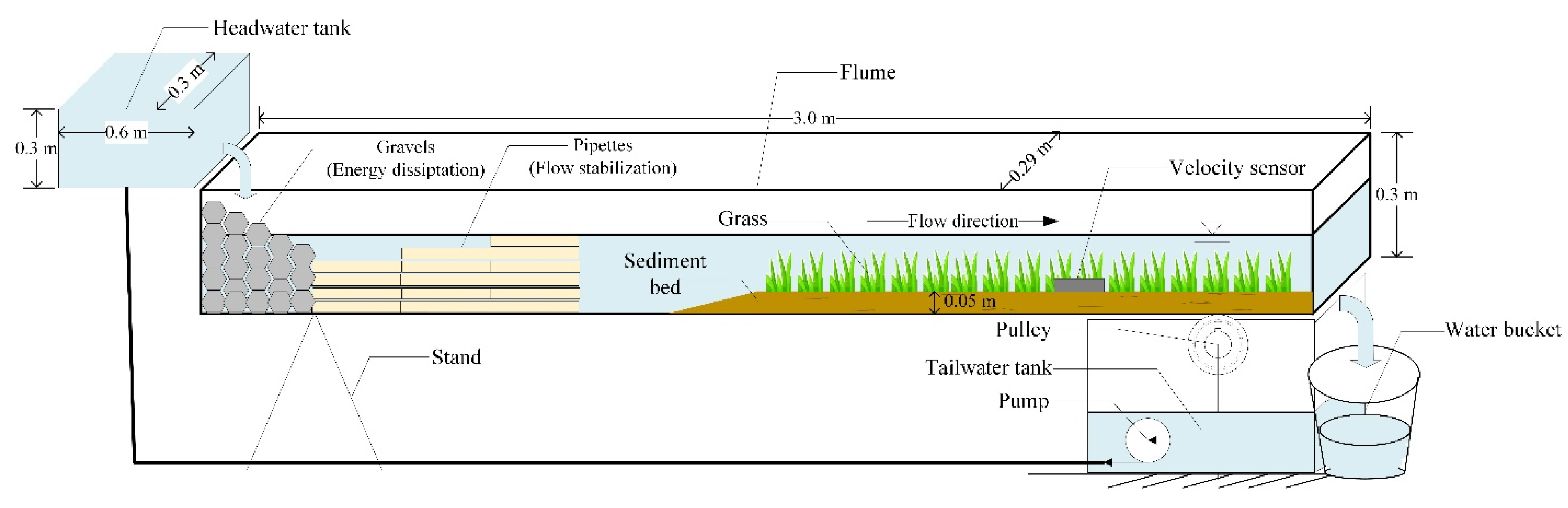
The flume apparatus used in the experiments discussed consisted of a recirculating rectangular flume, headwater tank, tailwater tank, and water bucket. The setup and dimensions of the apparatus are shown in Figure 1. The slope of the flume was adjusted by an electronic slope meter, and the steady water head in the headwater tank provided a constant water flow. To compare the different flow velocity measuring approaches, the PCM3 ultrasonic-type current meter developed by Nivus and the VM801-HS electromagnetic-type current meter developed by Kenek were used. The velocity sensor of the ultrasonic current meter was installed on the bed surface and used to measure the average velocity. The velocity measuring range of the sensor was from 0 to 6 m/s with an error of around 1%. The electromagnetic current meter was used to measure the point flow velocity at different depths, and its velocity measuring range was 0 to 2.5 m/s with an error of around 5 mm/s.

The grass species used in the flume experiments were Centipede grass (Eremochloa ophiuroides), Bermuda grass (Cynodon dactylon), and Carpet grass (Axonopus), which are commonly applied as the plant species in grassed channels. Centipede grass is a perennial bunchgrass that prefers acid soil and grows on hillslopes, pastures, and roadsides. In the red soil terrace in northern Taiwan, Centipede grass grows naturally as passivated grassland. As the sod of Centipede grass grows well and extensive management can be applied, the area of application has been increased and it has become one of the choices for grass seed spray on hillslopes. Bermuda grass is a perennial grass that is distributed in areas with sea levels below 600 m, and it can grow in acid and alkaline soil on sunny slopes, roadsides, riverbanks, grasslands, and sandy lands in coastal areas. It is a common grass seed spray species used for soil and water conservation on slopes, and it is applied on land grading slopes, embankments, and dikes. Some other general usage includes sod in gardens and sports fields. Carpet grass is a shade-tolerant perennial grass that prefers acid soil and grows in areas at elevations below 2000 m in Taiwan. It can be used as pasture and sod and is one of the main species used for grass seed spray on slopes for soil and water conservation purposes [3].

2.2. Experimental Procedure

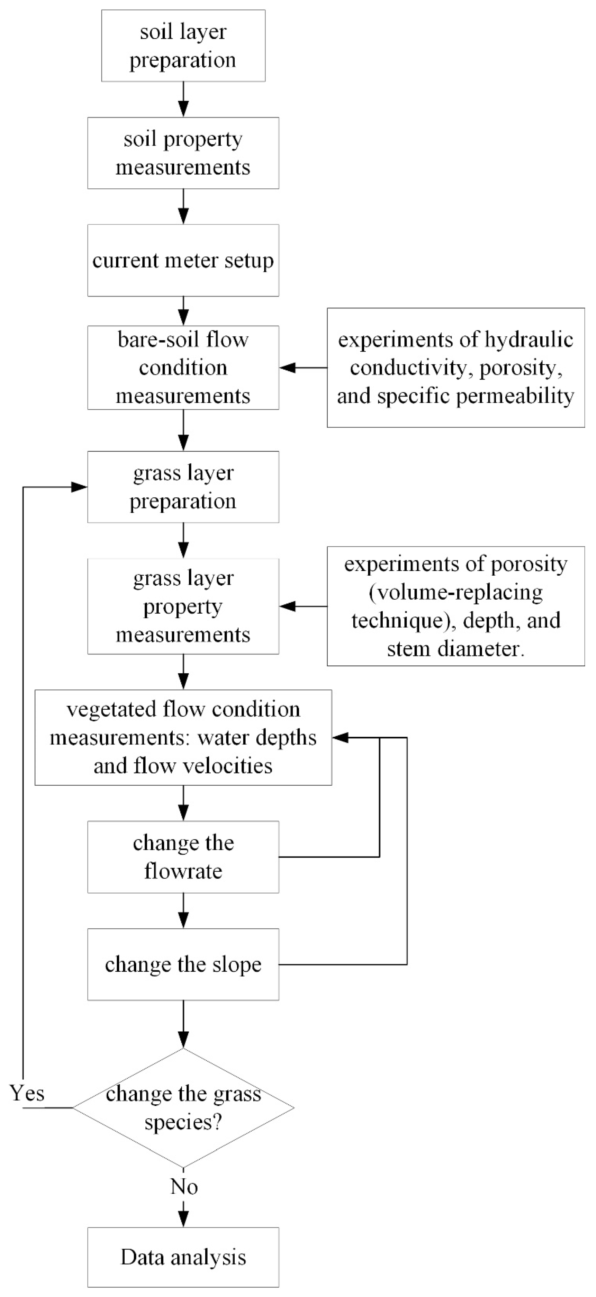
The experimental procedure of the grassed flume experiments is illustrated in Figure 2. During the experiments, the average velocity and flow velocities along the profile at different depths were measured by the ultrasonic and the electromagnetic current meters, respectively. The experimental steps include: (1) Spreading a layer of 0.05 m-deep red soil evenly on the flume bottom; (2) taking soil specimens and measuring the saturated hydraulic conductivity ($k$) and porosity ($n_3$) of the red soil; (3) installing the velocity sensor and setting up the data acquisition system for the current meters; (4) measuring the flow velocities under the bare-soil bed conditions for the calibration of the current meter; (5) spreading and planting the grass on the soil bed; (6) measuring the porosity ($n_2$) and depth ($h_2$) of the grass layer, as well as the average grass stem diameter ($d_c$); (7) turning on the inlet valve, then measuring and recording the water depths and flow velocities; (8) changing to another flowrate, then repeating step (7); (9) changing to anther slope and then repeating steps (7) and (8); (10) changing to another grass species and repeating steps (5) to (9). In this study, we applied three bed slopes, four heights of grass relative to the water depth, and three grass species. Therefore, a total of 36 complete test runs were conducted.

2.3. Measurements of Soil Layer Properties

The saturated hydraulic conductivity of the red soil was measured by the measuring apparatus manufactured by Eijkelkamp (Brochure no.4/09.02.01.05). Based on Darcy’s law, the saturated hydraulic conductivity of the soil specimen, k ($\mathrm{m}/\mathrm{day}$), can be calculated as:

$$k=\frac{Q^{\prime }\times L}{\Delta H\times A^{\prime }}$$

(3)

where $Q^{\prime }=$ outflow through the soil specimen (${\mathrm{m}}^3/\mathrm{day}$); $L=$ soil specimen height ($\mathrm{m}$); $\Delta H=$ hydraulic head difference ($\mathrm{m}$); $A^{\prime }=$ cross-sectional area of soil specimen (${\mathrm{m}}^2$). Then, the specific permeability (k_p3) can be calculated by the formula:

$$k_{p3}=\frac{\mu k}{\gamma }$$

(4)

where $\mu =$ kinematic viscosity coefficient of water ($\mathrm{N}·\mathrm{s}/{\mathrm{m}}^2$) and $\gamma =$ specific gravity of water ($\mathrm{N}/{\mathrm{m}}^3$). In this study, the porosity (n₃) and specific permeability (k_p3) of the red soil layer were 0.602 and 1.392 × 10⁻¹² (${\mathrm{m}}^2$), respectively.

2.4. Measurements of Grass Layer Properties

For the grass layer, the parameters of the porosity (n₂), depth (h₂), and average grass stem diameter ($d_c$) were measured. The grass layer porosity (n₂) was measured based on the volume-replacing technique, and the steps included: (1) Selecting a control volume of the grass layer; (2) removing the roots below the soil surface to reduce measuring errors; (3) measuring and recording the length (l), width (w₂), and height (h₂) of the grass layer; (4) measuring and recording the average grass stem diameter ($d_c$); (5) putting the grass into a 1000 mL volumetric cylinder and adding water of a known volume (V₁); and (6) recording the graduation of the water surface in the cylinder (V₂) and using the following equation to calculate the grass layer porosity:

$$n_2=1-\frac{V_2-V_1}{l\times w_2\times h_2}$$

(5)

The specific permeability of vegetation (k_p2) can be calculated by the formula proposed by Kaviany (1991):

$$k_{p2}=\frac{{\left(n_2\right)}^3}{80{\left(1-n_2\right)}^2}\times d_c{}^2.$$

(6)

In this study, the measured grass layer parameters for the three grass species are listed in

Table 1. Selected parameters of the grass layer.

Grass Species	Parameters (Unit)	Values
Centipede grass (Eremochloa ophiuroides)	Height (m)	0.031
	Porosity (-)	0.715
	Specific permeability (m2)	1.765 × 10−7
	Manning’s n a (-)	0.055
Bermuda grass (Cynodon dactylon)	Height (m)	0.036
	Porosity (-)	0.947
	Specific permeability (m2)	2.941 × 10−7
	Manning’s n b (-)	0.05
Carpet grass (Axonopus)	Height (m)	0.041
	Porosity (-)	0.781
	Specific permeability (m2)	1.987 × 10−6
	Manning’s n a (-)	0.05

^a Values of Manning’s n were assigned based on the Soil and Water Conservation Handbook [3]. ^b Value of Manning’s n was estimated based on [2,19].

.

2.5. Flow Velocity Measurements

2.5.1. Ultrasonic Current Meter

The Nivus PCM3 ultrasonic current meter was used to measure the average flow velocity in the flume. During the flume experiments, the velocity sensor was installed on the bed in the downstream area of the flume where the flow condition was relatively steady. When measuring the flow velocity, the velocity sensor had to be covered in the water layer at all times to reduce the measuring errors. Then, the measured velocity (${\overline{V}}_{ultra}$) could be read out from the data acquisitor of the ultrasonic current meter. The calibration of the ultra-magnetic current meter was carried out by following the manufacturers’ guidelines before the experiments. The measuring range of the ultrasonic current meter was 0 to 6 m/s, with an average error of 1%.

2.5.2. Electromagnetic Current Meter

The Kenek VM801-HS electromagnetic current meter was used to measure the point velocity at different depths of a vertical line to obtain the flow velocity profile. For each of the point velocities of a vertical profile measured by the electromagnetic current meter, we took the average value of at least three measurements at each point. The flow velocity profile described the flow conditions of different points along water depth, and the measured velocities could be used to calculate the average velocity (${\overline{V}}_{elect}$) as the following:

$${\overline{V}}_{elect}=\frac{V_1{h}_1+V_2{h}_2{n}_2}{h_1+h_2{n}_2}$$

(7)

where $V_1=$ the flow velocity in the water layer ($\mathrm{m}/\mathrm{s}$); $V_2=$ the flow velocity in the grass layer ($\mathrm{m}/\mathrm{s}$); $h_1=$ the depth of the water layer ($\mathrm{m}$); $n_2=$ the porosity of the grass layer. Calibrations of the electromagnetic current meter were carried out by following the manufacturers’ guidelines before the experiments. The measuring range of the electromagnetic current meter was 0 to 2.5 m/s, with an average error of 5 mm/s.

2.5.3. The Bucket Method

The bucket method was used to calculate the average velocity by dividing the flowrate measurement by the cross-sectional area in the flume. The actual cross-sectional area of flow in the grass layer was estimated by multiplying the grass layer cross-sectional area and the grass layer porosity. The average velocity (${\overline{V}}_{bucket}$) estimated from the bucket method can be calculated as:

$${\overline{V}}_{bucket}=\frac{Q_b}{b\left(h_1+h_2{n}_2\right)},$$

(8)

where $Q_b=$ the flowrate measured by the bucket method (${\mathrm{m}}^3/\mathrm{s}$) and $b=$ width of the flume ($\mathrm{m}$). Since ${\overline{V}}_{bucket}$ was obtained by the measured flowrate and the actual flow cross-sectional area, which accounted for the water and grass layer, ${\overline{V}}_{bucket}$ was taken as the best velocity estimate of the actual average velocity in the flume.

2.5.4. Manning’s Equation

The average flow velocities obtained by the above methods were compared with the value calculated by Manning’s equation (${\overline{V}}_{Manning}$), which is:

$${\overline{V}}_{Manning}=\frac{1}{n}{R}^{2/3}{S}^{1/2}.$$

(9)

where $S=$ the slope of the water surface under uniform flow, which can be replaced by the bed slope.

2.5.5. Analytical Solution for Water Flow Passing a Grass Layer

The average flow velocity (${\overline{V}}_{anal}$) was also calculated based on the analytical method for measuring the flow velocity in grassed channels proposed by Hsieh and Shiu [30]. Based on their theory, the flow field is divided into three regions: Region I contains only the homogeneous fluid (the water layer), region II contains grass and homogeneous fluid (the grass layer), and region III is the permeable saturated soil layer (the soil layer). The flow velocities corresponding to the three layers were obtained by the analytical solutions to the partial differential equations of the flow field. The main equations for calculating the flow velocities in the water layer (V_{1_anal}) and grass layer (V_{2_anal}) are shown as follows:

$${\overline{V}}_{anal}=\frac{{\int }_{h_2}^{h_1+h_2}{V}_{1\_anal}dy+{\int }_0^{h_2}{V}_{2\_anal}dy}{h_1+h_2{n}_2}.$$

(10)

$$\begin{gathered} V_{1\_anal}\left(y\right)=\frac{{\rho }_{w}g\sin \theta }{\mu }·\{\frac{\mu \left(\mu +\beta \sqrt{\sin \theta }\right){\left(h_1+h_2\right)}^2}{{\beta }^2\sin \theta }·\ln \left(1+\frac{\beta \sqrt{\sin \theta }}{\mu \left(h_1+h_2\right)}y\right)-\frac{\mu \left(h_1+h_2\right)}{\beta \sqrt{\sin \theta }}y+ \\ \frac{{\mu }^2{\left(h_1+h_2\right)}^2}{{\beta }^2\sin \theta }-\frac{\mu \left(\mu +\beta \sqrt{\sin \theta }\right){\left(h_1+h_2\right)}^2}{{\beta }^2\sin \theta }·\ln \left(1+\frac{\beta \sqrt{\sin \theta }{h}_2}{\mu \left(h_1+h_2\right)}\right)+\frac{\mu \left(h_1+h_2\right)h_2}{\beta \sqrt{\sin \theta }}+\frac{n_2^3{d}_c^2}{80{\left(1-n_2\right)}^2}+ \\ {C}_1{h}_1\frac{B_1}{B_3}\frac{n_2{d}_c}{\sqrt{80}\left(1-n_2\right)}+\frac{\left(B_1{B}_4+B_2{B}_3\right)}{B_3}·\frac{C_1{h}_1{C}_2+C_3}{C_4}\}\hspace{1em}\hspace{1em}\mathrm{for}{h}_2\le y\le h_1+h_2 \end{gathered}$$

(11)

$$\begin{gathered} V_{2\_anal}\left(y\right)=\frac{{\rho }_{w}g\sin \theta }{\mu }·\{\frac{n_2{d}_c^2}{80{\left(1-n_2\right)}^2}+I_0·(\frac{C_1{h}_1{C}_2+C_3}{C_4}+\frac{C_1{h}_1{n}_2{d}_c}{\sqrt{80B_3}\left(1-n_2\right)})· \\ \left(2\sqrt{n_2\mu \left(h_1+h_2\right)}\sqrt{\frac{\mu \left(h_1+h_2\right)\beta \sqrt{\sin \theta }y}{k_{p2}{\beta }^2\sin \theta }}\right)+K_0·(\frac{C_1{h}_1{C}_2+C_3}{C_4})· \\ \left(2\sqrt{n_2\mu \left(h_1+h_2\right)}\sqrt{\frac{\mu \left(h_1+h_2\right)\beta \sqrt{\sin \theta }y}{k_{p2}{\beta }^2\sin \theta }}\right)\}\hspace{1em}\hspace{1em}\mathrm{for}0\le y\le h_2 \end{gathered}$$

(12)

where $y=$ depth from the soil layer surface (m); $\theta =$ the slope of channel; ${\rho }_w=$ density of water ($\mathrm{kg}/{\mathrm{m}}^3$); $I_0=$ the 0th modified Bessel function of the first kind; $K_0=$ the 0th modified Bessel function of the second kind; $\beta ,B_1,B_2,B_3,B_4,C_1,C_2,C_3,C_4=$ coefficients of the analytical solutions detailed in Hsieh and Shiu [30].

3. Results

3.1. Average Flow Velocities with Different Relative Heights

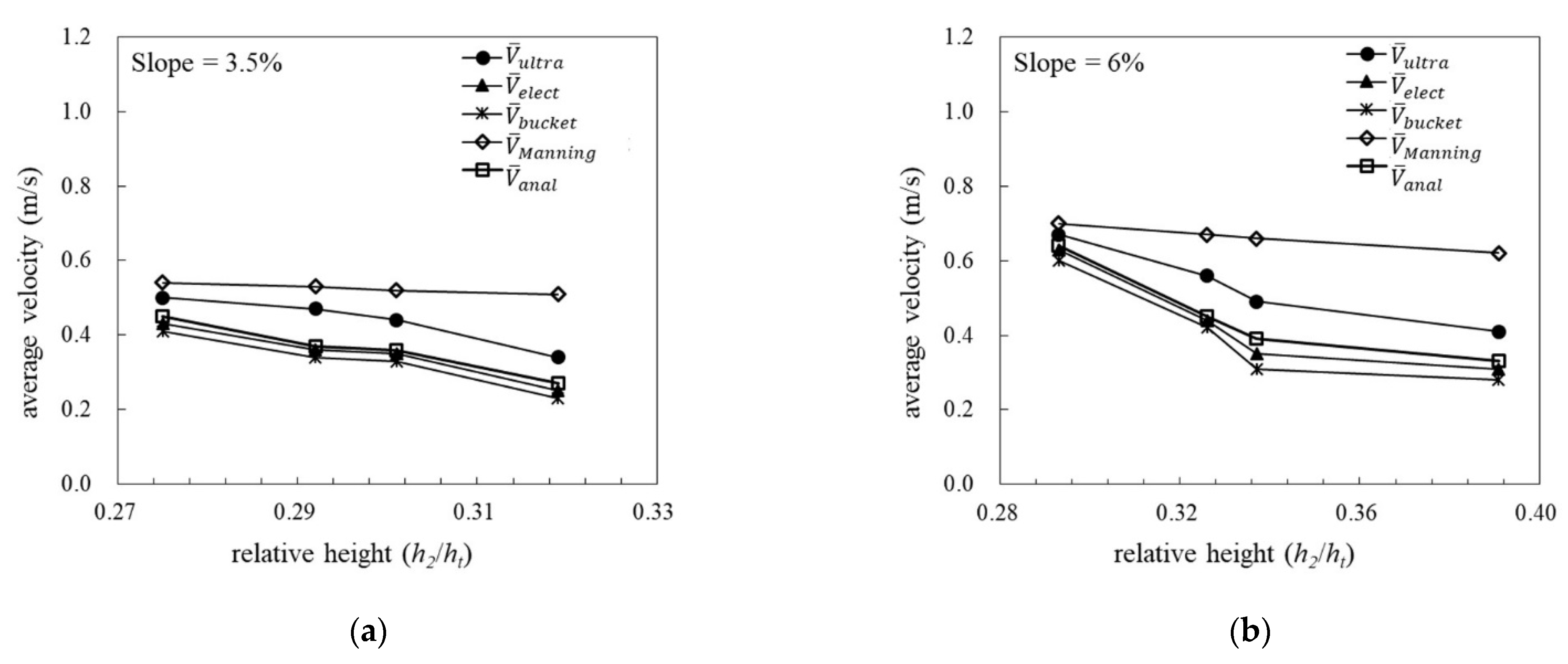
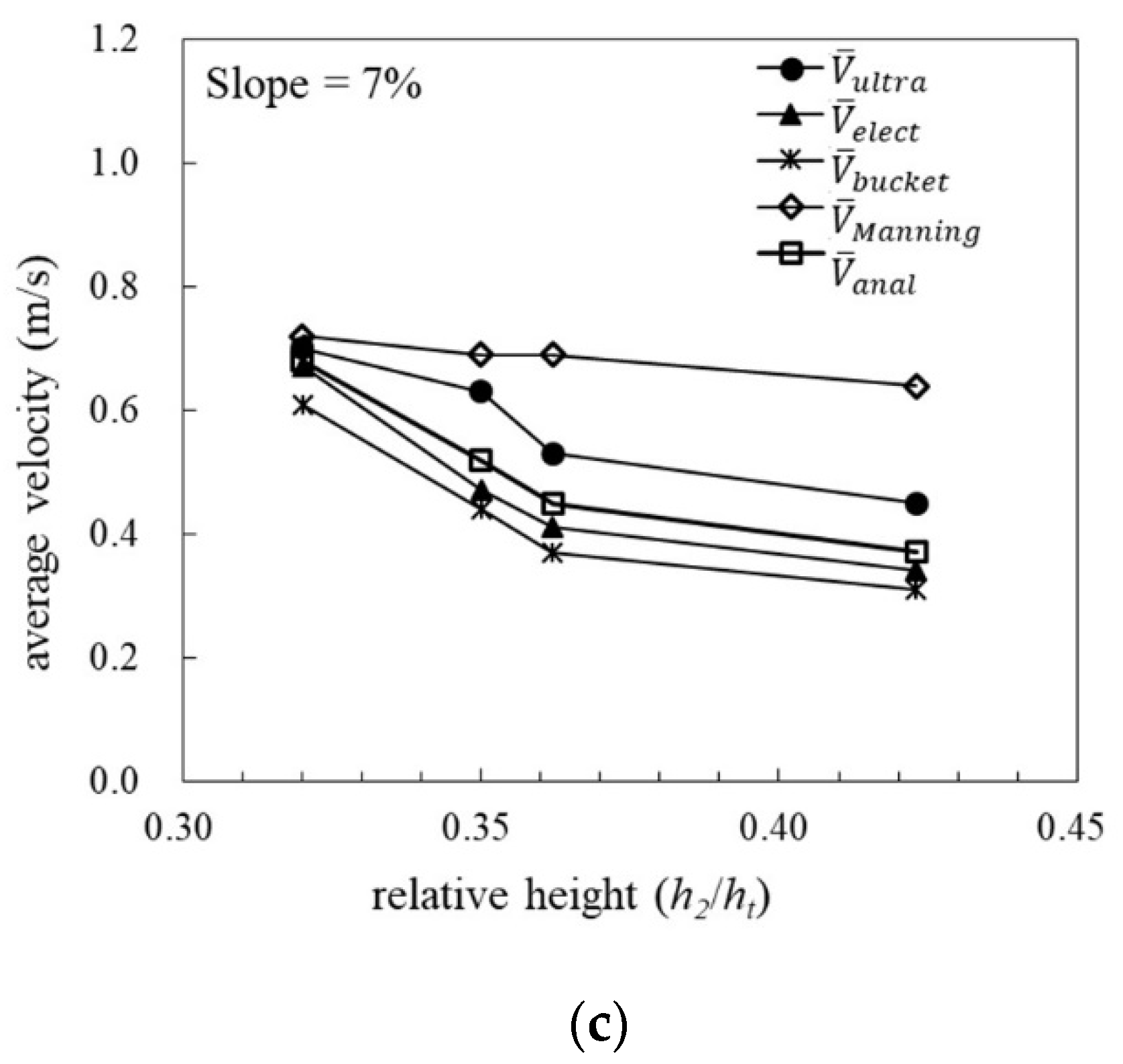
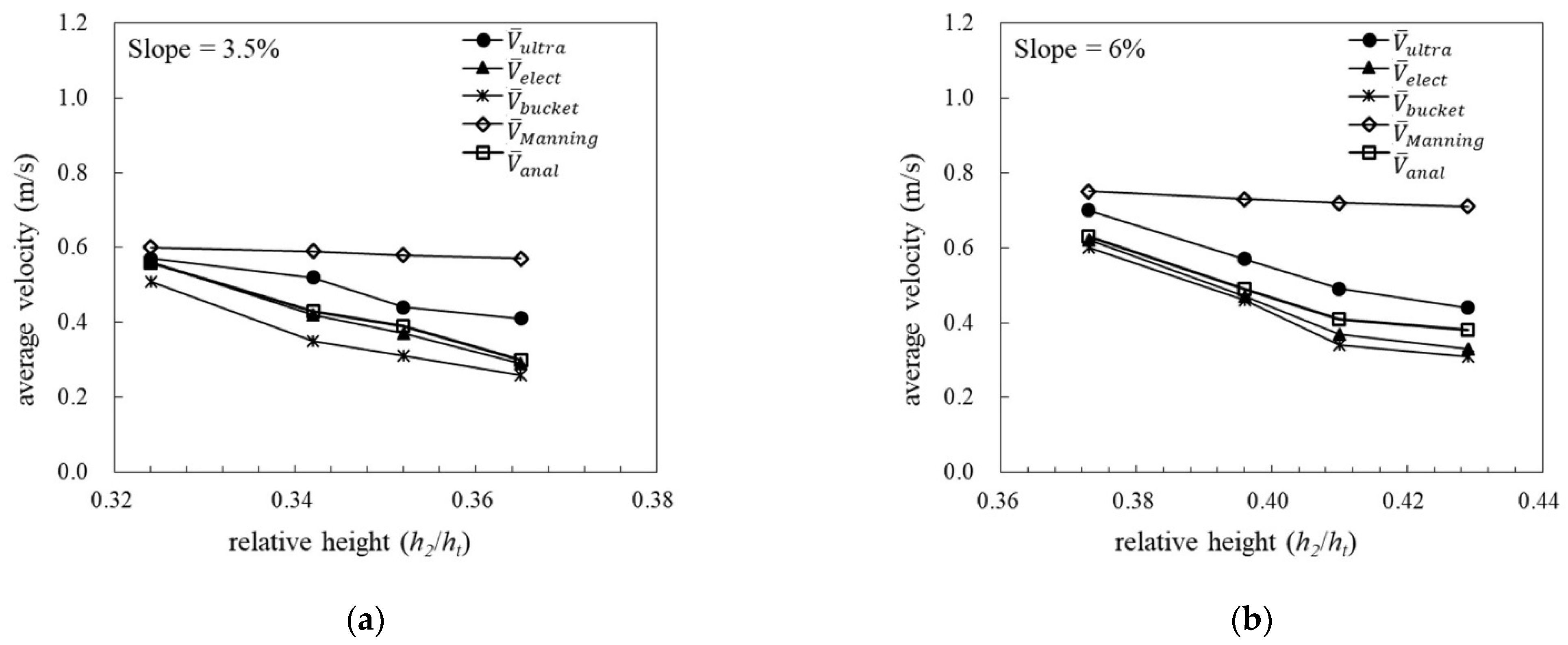
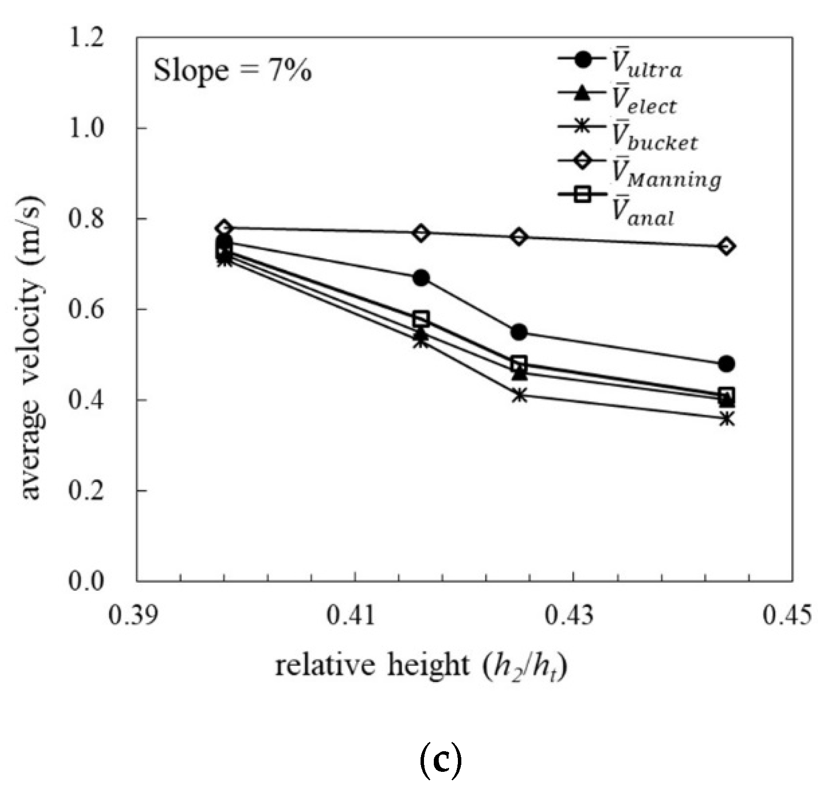
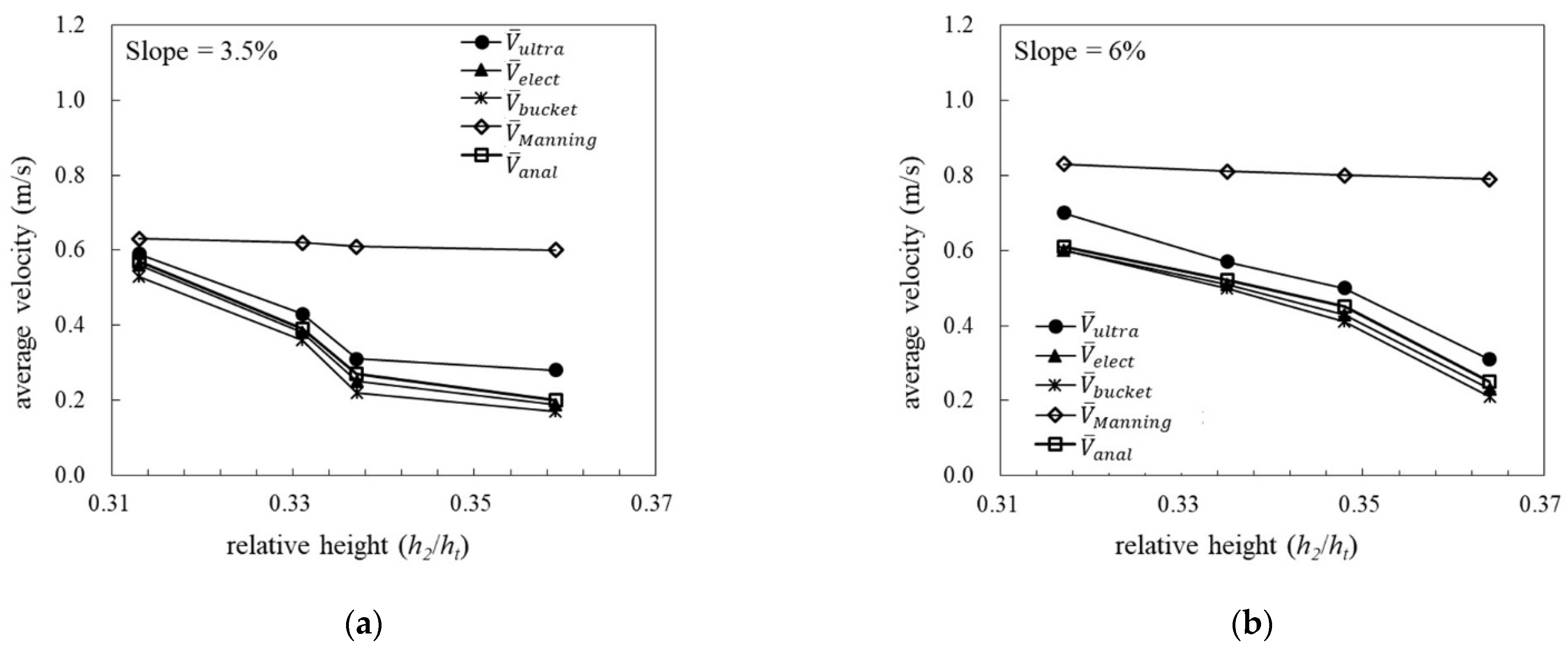
The average flow velocities in the grassed flume, measured by the ultrasonic current meter (${\overline{V}}_{ultra}$), the electromagnetic current meter (${\overline{V}}_{elect}$), and the bucket method (${\overline{V}}_{bucket}$) and calculated by Manning’s equation (${\overline{V}}_{Manning}$) and the analytical method (${\overline{V}}_{anal}$), with different relative heights for the three species of grass, are shown in Figure 3, Figure 4 and Figure 5. The relative height—i.e., $h_2/\left(h_1+h_2\right)$—was controlled by the flowrate and bed slope. Since $h_2$ was fixed for each grass species (Table 1), $h_2/\left(h_1+h_2\right)$ decreased as the flowrate and thus $h_1$ increased. For all three grass species (Figure 3, Figure 4 and Figure 5), in the case of the same slope, the flow velocity evaluated by each method increased as the relative height decreased. As the flume slope varied from 3.5, 6, to 7%, the flow velocities at different relative heights generally increased with the slope for all the evaluating methods. The comparison among the results of different evaluating methods shows that ${\overline{V}}_{Manning}>{\overline{V}}_{ultra}>{\overline{V}}_{anal}>{\overline{V}}_{elect}>{\overline{V}}_{bucket}$; the variation trends of ${\overline{V}}_{anal}$, ${\overline{V}}_{elect}$, and ${\overline{V}}_{bucket}$ with the relative height were similar and close to one another. In order to show the fluctuation of average velocity measurements varied with the relative height of each method, we calculated the “total increment of average velocity of each method”, which was the difference between the largest and the smallest average velocity divided by the smallest average velocity. For example, in Figure 5a for the tests of the carpet grass with the slope set at 3.5%, when the relative height was 0.359, the average velocity measured by the bucket method was 0.170 (m/s)—i.e., ${\overline{V}}_{bucket}=0.170$. When the relative height was 0.313, the average velocity measured by the bucket method was 0.530 (m/s)—i.e., ${\overline{V}}_{bucket}=0.530$. Therefore, the “total increment of average velocity of the bucket method” in this case was (0.530–0.170)/0.170 = 212%—i.e., ${\overline{V}}_{bucket}$(212%). To show the average velocity differences measured/estimated by the various methods comparing with the values of the bucked method,

Table 2. Differences in the average velocities obtained from the different methods comparing with the bucket method.

Grass Species	Slope (%)	$$\begin{gathered} {\overline{\mathit{V}}}_{\mathit{u}\mathit{l}\mathit{t}\mathit{r}\mathit{a}}-{\overline{\mathit{V}}}_{\mathit{b}\mathit{u}\mathit{c}\mathit{k}\mathit{e}\mathit{t}} \\ (\mathbf{m}/\mathbf{s}) \end{gathered}$$	$$\begin{gathered} {\overline{\mathit{V}}}_{\mathit{e}\mathit{l}\mathit{e}\mathit{c}\mathit{t}}-{\overline{\mathit{V}}}_{\mathit{b}\mathit{u}\mathit{c}\mathit{k}\mathit{e}\mathit{t}} \\ (\mathbf{m}/\mathbf{s}) \end{gathered}$$	$$\begin{gathered} {\overline{\mathit{V}}}_{\mathit{M}\mathit{a}\mathit{n}\mathit{n}\mathit{i}\mathit{n}\mathit{g}}-{\overline{\mathit{V}}}_{\mathit{b}\mathit{u}\mathit{c}\mathit{k}\mathit{e}\mathit{t}} \\ (\mathbf{m}/\mathbf{s}) \end{gathered}$$	$$\begin{gathered} {\overline{\mathit{V}}}_{\mathit{a}\mathit{n}\mathit{a}\mathit{l}}-{\overline{\mathit{V}}}_{\mathit{b}\mathit{u}\mathit{c}\mathit{k}\mathit{e}\mathit{t}} \\ (\mathbf{m}/\mathbf{s}) \end{gathered}$$
Centipede grass	3.5	0.44	0.08	0.79	0.14
	6	0.52	0.12	1.04	0.20
	7	0.58	0.16	1.01	0.29
Bermuda grass	3.5	0.51	0.21	0.91	0.25
	6	0.49	0.08	1.20	0.20
	7	0.44	0.12	1.04	0.19
Carpet grass	3.5	0.33	0.10	1.18	0.15
	6	0.36	0.05	1.51	0.11
	7	0.25	0.08	1.38	0.11
RMSE		0.447	0.120	1.138	0.191

shows the velocity differences and root-mean-square deviations (RMSEs) of each method. The RMSE for the different measuring methods suggest the average errors in the flow velocity obtained by the other methods when the velocities measured by the bucket method are viewed as the observed values. Values of the RMSE show the same sequence as ${\overline{V}}_{Manning},{\overline{V}}_{ultra},{\overline{V}}_{anal},\mathrm{and}{\overline{V}}_{elect}$.

3.1.1. Velocity Variation in Cases of Centipede Grass

The results of the average flow velocities in cases of different relative heights obtained by the five evaluating methods in the grassed flume with the Centipede grass layer are shown in Figure 3. When the slope was set at 3.5% (Figure 3a), the relative height varied from 0.319 to 0.275 as the flowrate increased, and the average flow velocity increased as the relative height decreased. The ranking of the total increment in average velocity for each method was ${\overline{V}}_{bucket}$(78%) > ${\overline{V}}_{elect}$(72%) > ${\overline{V}}_{anal}$(67%) > ${\overline{V}}_{ultra}$(47%) > ${\overline{V}}_{Manning}$(6%). When the slope was set at 6% (Figure 3b), the relative height varied from 0.391 to 0.293, and the ranking of the total increment in average velocity for each method was ${\overline{V}}_{bucket}$(114%) > ${\overline{V}}_{elect}$(103%) > ${\overline{V}}_{anal}$(94%) > ${\overline{V}}_{ultra}$(63%) > ${\overline{V}}_{Manning}$(13%). When the slope was set at 7% (Figure 3c), the relative height varied from 0.423 to 0.320 and the ranking of the total increment in average velocity for each method was ${\overline{V}}_{bucket}$(97%) $\approx$ ${\overline{V}}_{elect}$(97%) > ${\overline{V}}_{anal}$(84%) > ${\overline{V}}_{ultra}$(56%) > ${\overline{V}}_{Manning}$(13%). In summary, the relative height increased as the slope increased, which indicated that the total water depth was decreasing as the slope was increasing. For the velocity variation between different relative heights, ${\overline{V}}_{bucket}$ showed the highest value and the variations in ${\overline{V}}_{elect}$ and ${\overline{V}}_{anal}$ showed similar values. In contrast, ${\overline{V}}_{Manning}$ showed the smallest velocity variation, which suggested that ${\overline{V}}_{Manning}$ was the least affected by the relative height.

3.1.2. Velocity Variation in Cases of Bermuda Grass

The results of the average flow velocities in cases of different relative heights obtained by the five evaluating methods in the grassed flume with a Bermuda grass layer are shown in Figure 4. When the slope was set at 3.5% (Figure 4a), the relative height varied from 0.365 to 0.324 as the flowrate increased, and the average flow velocity increased as the relative height decreased. The ranking of the total increment in average velocity for each method was ${\overline{V}}_{bucket}$(96%) > ${\overline{V}}_{elect}$(93%) > ${\overline{V}}_{anal}$(87%) > ${\overline{V}}_{ultra}$(39%) > ${\overline{V}}_{Manning}$(5%). When the slope was set at 6% (Figure 4b), the relative height varied from 0.429 to 0.373, and the ranking of the total increment in average velocity for each method was ${\overline{V}}_{bucket}$(94%) > ${\overline{V}}_{elect}$(88%) > ${\overline{V}}_{anal}$(66%) > ${\overline{V}}_{ultra}$(59%) > ${\overline{V}}_{Manning}$(6%). When the slope was set at 7% (Figure 4c), the relative height varied from 0.444 to 0.398, and the ranking of the total increment in average velocity for each method was ${\overline{V}}_{bucket}$(97%) > ${\overline{V}}_{elect}$(80%) > ${\overline{V}}_{anal}$(78%) > ${\overline{V}}_{ultra}$(56%) > ${\overline{V}}_{Manning}$(5%). In the Bermuda grassed flow experiments, the relationships between the relative height, slope, and velocity variation can be ascertained similarly to those in the cases of the Centipede grassed flow.

3.1.3. Velocity Variation in Cases of Carpet Grass

The results of the average flow velocities in the cases of the different relative heights obtained by the five evaluating methods in the grassed flume with a Carpet grass layer are shown in Figure 5. When the slope was set at 3.5% (Figure 5a), the relative height varied from 0.359 to 0.313 as the flowrate increased, and the average flow velocity increased as the relative height decreased. The ranking of the total increment in average velocity for each method was ${\overline{V}}_{bucket}$(212%) > ${\overline{V}}_{elect}$(195%) > ${\overline{V}}_{anal}$(185%) > ${\overline{V}}_{ultra}$(111%) > ${\overline{V}}_{Manning}$(5%). When the slope was set at 6% (Figure 5b), the relative height varied from 0.364 to 0.317, and the ranking of the total increment in average velocity for each method was ${\overline{V}}_{bucket}$(186%) > ${\overline{V}}_{elect}$(161%) > ${\overline{V}}_{anal}$(144%) > ${\overline{V}}_{ultra}$(126%) > ${\overline{V}}_{Manning}$(5%). When the slope was set at 7% (Figure 5c), the relative height varied from 0.393 to 0.346, and the ranking of the total increment in average velocity for each method was ${\overline{V}}_{anal}$(174%) > ${\overline{V}}_{elect}$(170%) > ${\overline{V}}_{bucket}$(169%) > ${\overline{V}}_{ultra}$(160%) > ${\overline{V}}_{Manning}$(5%). In the Carpet grassed flow experiments, relationships between the relative height, slope, and velocity variation showed similar trends as those in the cases of the Centipede grassed and Bermuda grassed flumes, except for the case of the steepest (7%) flume slope. In addition, the total increments in average velocity for most of the evaluating methods, except for Manning’s equation, were larger than 100% or even over 200%. This result suggested that Carpet grass was effective in flow deceleration, especially under high flowrate conditions with large relative heights.

3.2. Velocity Profiles with Different Grass Species

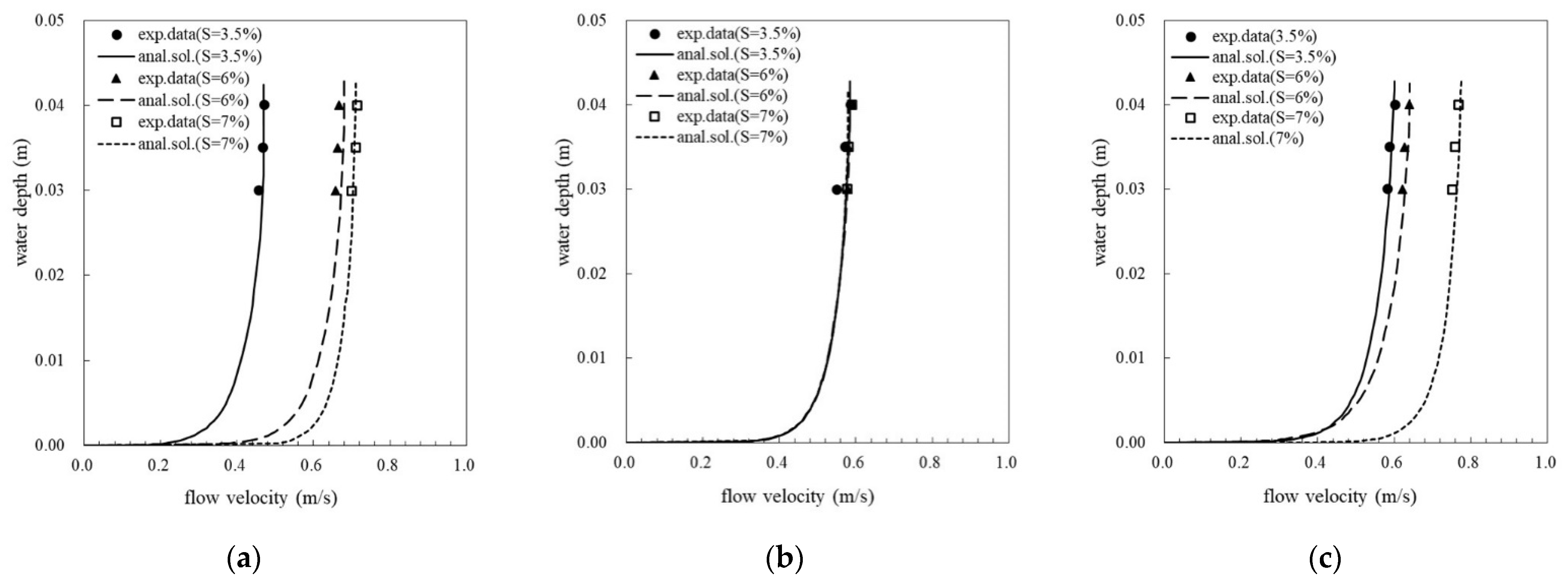
To investigate the flow velocity at different depths, the velocity profiles shown in Figure 6 were obtained by the measured data and the analytical solution for a selected cross-section in a downstream area of the flume where the flow was relatively steady. The flow velocities were measured at heights of 3, 3.5, and 4 cm from the bed, respectively, by the electromagnetic current meter. Under the flow conditions with different slopes and different species of the grass layer, the measured point velocities at different water depths fit the analytical solutions of the velocity profiles pretty well, even though only three measured points were obtained for each profile. When we compared the velocity profiles in the cases of different slopes, the flows with Centipede grass and Carpet grass as the grass layers both showed increasing trends of point velocity at a specific water depth as the slope increased. Therefore, the water velocity profile shifted to the right when the slope varied from 3.5 to 6 and 7% (Figure 6a,c). In contrast, in the Bermuda grassed flow the measured point velocities and velocity profiles in cases of different slopes varied slightly and nearly contracted to one another (Figure 6b). The average grass stem diameter ($\approx 0.1\mathrm{cm}$) of Bermuda grass was the smallest among the three grass species, which might have led to the difference in the velocity profile compared to the cases with the other two grass species.

4. Discussion

4.1. Comparison of Average Flow Velocity among the Three Grass Species

In the cases of all three slopes, Manning’s equation gave the largest flow velocity value for each relative height. However, the range of increase of ${\overline{V}}_{Manning}$ was between 5 and 13% (mostly from 5 to 6%) and was the smallest among all the evaluating methods as the grass layer height decreased. This result indicated that in the experiments, Manning’s equation was unable to reflect the effect of the interaction between the grass layer and water depth on the average velocity, while the other evaluating methods were able to. Particularly in cases of high relative heights, Manning’s equation tended to overestimate the average velocity. In contrast, the analytical solution for water flow passing a grass area resulted in similar average velocities to the values of the bucket method, which suggested that the analytical solution could reflect the correlation between the grass layer and water depth and give a more precise velocity estimation than Manning’s equation could.

If we compare the average velocities of flow conditions with similar relative heights among cases of the three grass species, it is found that in cases of lower relative heights (say, $h_2/\left(h_1+h_2\right)<0.36$), the flow conditions with Bermuda grass (Figure 4) showed the highest flow velocities among the three. This was followed by the average velocities for Carpet grass (Figure 5), and then those for Centipede grass (Figure 3). When the relative height became higher (say, $h_2/\left(h_1+h_2\right)>0.36$), the flow conditions with Bermuda grass (Figure 4) remained to show the highest flow velocities, followed by the velocities with Centipede grass (Figure 3) and then those with Carpet grass (Figure 5). According to the results of velocity variation with the relative height, Centipede grass or Carpet grass might show the best flow decelerating effects among the three grass species, but Bermuda grass showed the lowest flow decelerating effect. Therefore, when the design purpose was to decelerate flow and enhance water infiltration, and thus lower flow velocities are desired, Centipede grass or Carpet grass may be the most effective grassed channel cover, depending on the water depth and slope. If the main purpose is to release flooding and, thus, a higher flow velocity and flowrate are preferred, Bermuda grass may be the best choice for grassed channels.

4.2. Comparison between Measured Values and the Analytical Solution of Average Flow Velocity

For comparing the average flow velocity measured by the bucket method, the ultrasonic current meter, and the electromagnetic current meter with the analytical solution of the velocity proposed by Hsieh and Shiu [30], the ratios between the measured and analytical values are shown in

Table 3. Velocity ratios of measured values to the analytical values.

Grass Species	Slope	$\frac{{\mathit{h}}_2}{{\mathit{h}}_1+{\mathit{h}}_2}$	$\frac{{\overline{\mathit{V}}}_{\mathit{b}\mathit{u}\mathit{c}\mathit{k}\mathit{e}\mathit{t}}}{{\overline{\mathit{V}}}_{\mathit{a}\mathit{n}\mathit{a}\mathit{l}}}$	$\frac{{\overline{\mathit{V}}}_{\mathit{u}\mathit{l}\mathit{t}\mathit{r}\mathit{a}}}{{\overline{\mathit{V}}}_{\mathit{a}\mathit{n}\mathit{a}\mathit{l}}}$	$\frac{{\overline{\mathit{V}}}_{\mathit{e}\mathit{l}\mathit{e}\mathit{c}\mathit{t}}}{{\overline{\mathit{V}}}_{\mathit{a}\mathit{n}\mathit{a}\mathit{l}}}$
Centipede grass	3.5%	0.319	0.85	1.25	0.92
		0.301	0.91	1.22	0.97
		0.292	0.93	1.28	0.98
		0.275	0.92	1.12	0.96
	6%	0.391	0.84	1.23	0.93
		0.337	0.80	1.26	0.90
		0.326	0.93	1.23	0.97
		0.293	0.93	1.04	0.98
	7%	0.423	0.83	1.20	0.91
		0.362	0.82	1.18	0.91
		0.350	0.85	1.22	0.91
		0.320	0.90	1.03	0.99
Bermuda grass	3.5%	0.365	0.86	1.36	0.96
		0.352	0.79	1.12	0.94
		0.342	0.82	1.22	0.98
		0.324	0.91	1.02	1.00
	6%	0.429	0.81	1.14	0.86
		0.410	0.84	1.21	0.91
		0.396	0.95	1.17	0.97
		0.373	0.95	1.10	0.98
	7%	0.444	0.87	1.16	0.97
		0.425	0.85	1.14	0.95
		0.416	0.91	1.15	0.94
		0.398	0.97	1.03	0.99
Carpet grass	3.5%	0.359	0.84	1.39	0.94
		0.337	0.82	1.15	0.93
		0.331	0.92	1.09	0.97
		0.313	0.93	1.04	0.98
	6%	0.364	0.84	1.24	0.92
		0.348	0.92	1.12	0.96
		0.335	0.96	1.09	0.97
		0.317	0.99	1.15	0.99
	7%	0.393	0.95	1.10	0.98
		0.374	0.96	1.04	0.98
		0.368	0.93	1.08	0.98
		0.346	0.94	1.05	0.99

. Generally, no specific trends were found for the velocity ratios—i.e., ${\overline{V}}_{bucket}/{\overline{V}}_{anal}$, ${\overline{V}}_{ultra}/{\overline{V}}_{anal}$, and ${\overline{V}}_{elect}/{\overline{V}}_{anal}$—which showed variation with the grass species or slope. However, the velocity ratios of the different measuring methods to the analytical solution did show differences between the three: The values of ${\overline{V}}_{ultra}/{\overline{V}}_{anal}$ were always larger than one and had ranges of 1.02 to 1.39 (S = 3.5%), 1.04 to 1.26 (S = 6%), and 1.03 to 1.22 (S = 7%). The values of ${\overline{V}}_{elect}/{\overline{V}}_{anal}$ and ${\overline{V}}_{bucket}/{\overline{V}}_{anal}$ were always smaller than one but ${\overline{V}}_{elect}/{\overline{V}}_{anal}$ was closer to one. Specifically, the values of ${\overline{V}}_{elect}/{\overline{V}}_{anal}$ varied from 0.92 to 1.00 (S = 3.5%), 0.86 to 0.99 (S = 6%), and 0.91 to 0.99 (S = 7%); the values of ${\overline{V}}_{bucket}/{\overline{V}}_{anal}$ varied from 0.79 to 0.93 (S = 3.5%), 0.81 to 0.99 (S = 6%), and 0.82 to 0.97 (S = 7%). In each case, the average flow velocity measured by the electromagnetic current meter showed the closest, though smaller, value to the velocity obtained from the analytical solution.

4.3. Comparison between Measured Values and Manning’s Estimations of Average Flow Velocity

In order to compare the average flow velocity measured by the bucket method, the ultrasonic current meter, and the electromagnetic current meter with the velocity calculated by Manning’s equation, the ratios between the measured values and Manning’s velocity values are shown in

Table 4. Velocity ratios of measured values to Manning’s estimations.

Grass Species	Slope	$\frac{{\mathit{h}}_2}{{\mathit{h}}_1+{\mathit{h}}_2}$	$\frac{{\overline{\mathit{V}}}_{\mathit{b}\mathit{u}\mathit{c}\mathit{k}\mathit{e}\mathit{t}}}{{\overline{\mathit{V}}}_{\mathit{M}\mathit{a}\mathit{n}\mathit{n}\mathit{i}\mathit{n}\mathit{g}}}$	$\frac{{\overline{\mathit{V}}}_{\mathit{u}\mathit{l}\mathit{t}\mathit{r}\mathit{a}}}{{\overline{\mathit{V}}}_{\mathit{M}\mathit{a}\mathit{n}\mathit{n}\mathit{i}\mathit{n}\mathit{g}}}$	$\frac{{\overline{\mathit{V}}}_{\mathit{e}\mathit{l}\mathit{e}\mathit{c}\mathit{t}}}{{\overline{\mathit{V}}}_{\mathit{M}\mathit{a}\mathit{n}\mathit{n}\mathit{i}\mathit{n}\mathit{g}}}$
Centipede grass	3.5%	0.319	0.45	0.67	0.51
		0.301	0.63	0.84	0.52
		0.292	0.64	0.89	0.53
		0.275	0.76	0.93	0.54
	6%	0.391	0.45	0.66	0.50
		0.337	0.47	0.74	0.53
		0.326	0.63	0.84	0.66
		0.293	0.86	0.96	0.90
	7%	0.423	0.48	0.70	0.53
		0.362	0.54	0.77	0.60
		0.350	0.63	0.91	0.68
		0.320	0.85	0.97	0.93
Bermuda grass	3.5%	0.365	0.46	0.72	0.57
		0.352	0.54	0.76	0.58
		0.342	0.60	0.89	0.59
		0.324	0.85	0.95	0.60
	6%	0.429	0.44	0.62	0.47
		0.410	0.47	0.68	0.51
		0.396	0.63	0.78	0.65
		0.373	0.80	0.94	0.83
	7%	0.444	0.48	0.64	0.54
		0.425	0.54	0.73	0.61
		0.416	0.69	0.88	0.72
		0.398	0.91	0.96	0.92
Carpet grass	3.5%	0.359	0.28	0.47	0.60
		0.337	0.36	0.51	0.61
		0.331	0.58	0.69	0.62
		0.313	0.84	0.94	0.63
	6%	0.364	0.27	0.39	0.29
		0.348	0.51	0.63	0.54
		0.335	0.62	0.70	0.63
		0.317	0.72	0.84	0.72
	7%	0.393	0.32	0.37	0.33
		0.374	0.53	0.58	0.54
		0.368	0.68	0.79	0.71
		0.346	0.81	0.91	0.85

. Generally, all the velocity ratios—i.e., ${\overline{V}}_{bucket}/{\overline{V}}_{Manning}$, ${\overline{V}}_{ultra}/{\overline{V}}_{Manning}$, and ${\overline{V}}_{elect}/{\overline{V}}_{Manning}$—were smaller than one but became closer to one when the flow depth increased—i.e., $h_2/\left(h_1+h_2\right)$ decreased. In terms of the varying range, ${\overline{V}}_{ultra}/{\overline{V}}_{Manning}$ varied from 0.47 to 0.95 (S = 3.5%), 0.39 to 0.96 (S = 6%), and 0.37 to 0.97 (S = 7%); ${\overline{V}}_{elect}/{\overline{V}}_{Manning}$ varied from 0.51 to 0.63 (S = 3.5%), 0.29 to 0.90 (S = 6%), and 0.35 to 1.00 (S = 7%); and ${\overline{V}}_{bucket}/{\overline{V}}_{Manning}$ varied from 0.28 to 0.85 (S = 3.5%), 0.29 to 0.91 (S = 6%), and 0.33 to 0.92 (S = 7%). In summary, the three velocity ratios were close to one under large water depth conditions but much smaller than one when the water depth was small. The small values for the velocity ratio suggest that Manning’s equation overestimated the actual flow velocity, represented by the measured values, and thus was insensitive to the vegetation effect on flow velocity in cases of shallow water depths.

4.4. Application to Grassed Channel Design

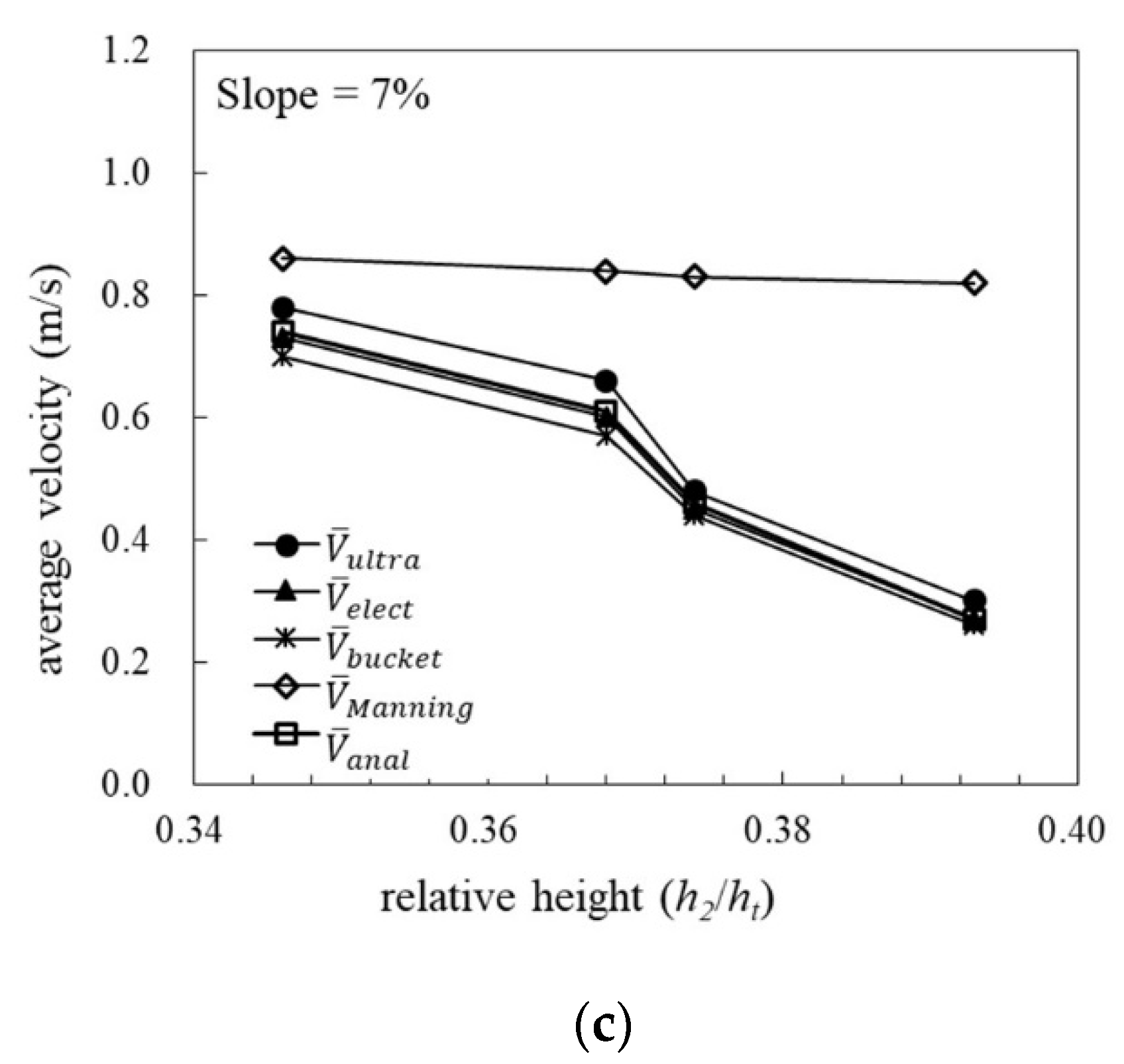
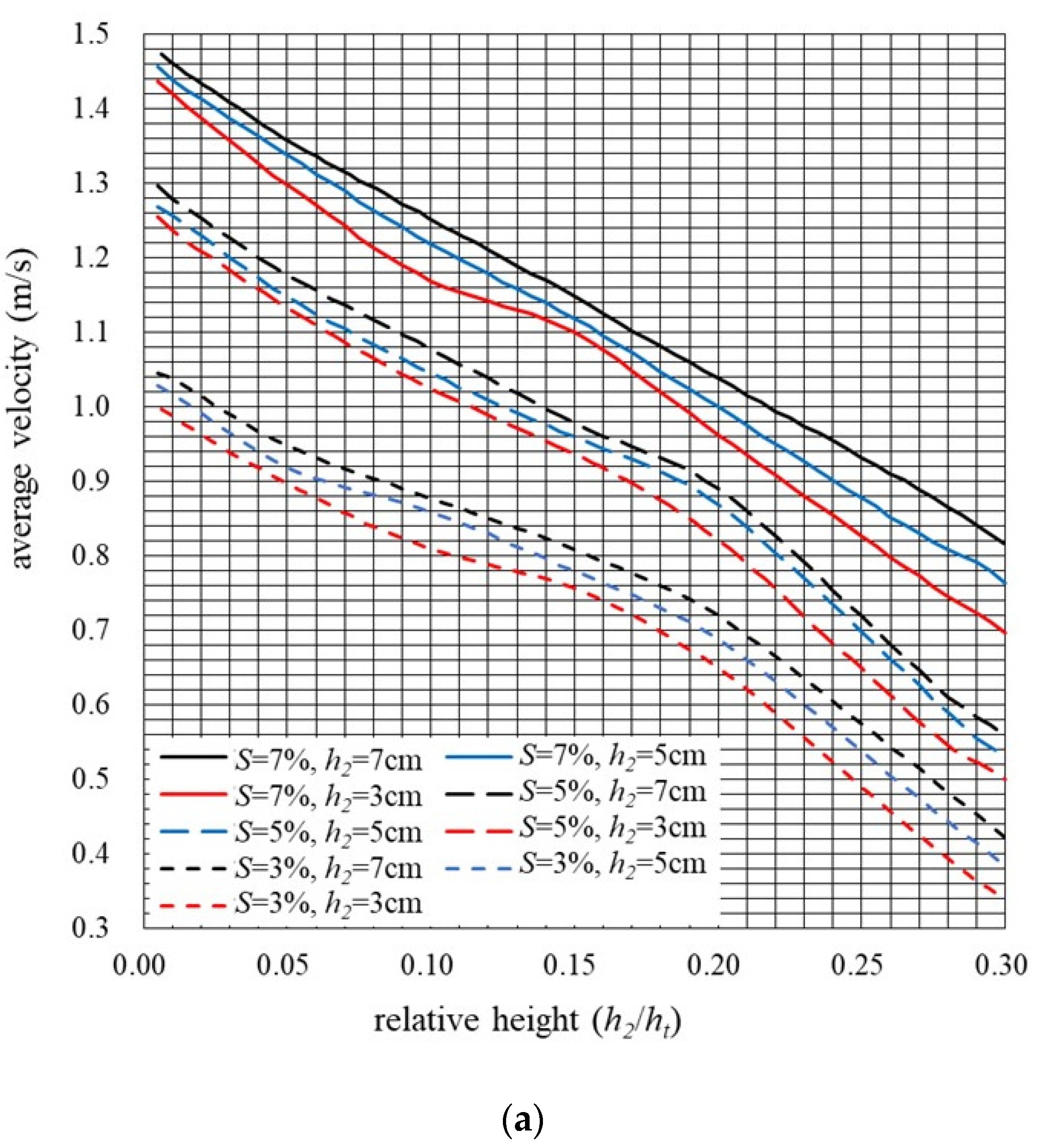
Most of the recent literature regarding the roughness characteristics of grassed channels focuses on the investigation and and/or modification of Manning’s n [24,25,26] or the friction factor [27,28,29]. In our experiment, the channel slope, density of vegetation, and relative grass height were all considered, as well as the soil characteristics, which shows that the present experimental study involves more factors related to vegetated flow. However, this study is not focused on the discussion of Manning’s roughness coefficient or the friction factor. The purpose of this study is to point out that the values of Manning’s n for the grassed channels suggested by the designing guideline and chosen by Taiwan’s engineers could lead to significant errors when designing flow velocity. Therefore, the relationships between the average flow velocity and the relative height in grassed channels with different bed slopes and the three grass species are proposed and shown in Figure 7. The analytical solutions of the grassed flow velocity were validated under the conditions of a bed slope less than 7% and grassed channels with a grass layer height less than 7 cm. With the measured grass layer porosities shown in

Table 5. Grass layer porosities for different heights and different grass species.

		Grass Species	Centipede Grass	Bermuda Grass	Carpet Grass
	Porosity
Height (m)
0.02			0.710	0.944	0.765
0.03			0.715	0.947	0.770
0.04			0.718	0.949	0.779
0.05			0.720	0.951	0.783
0.06			0.725	0.955	0.792
0.07			0.729	0.957	0.796

, the analytical solution can be applied to estimations of hydraulic characteristics for grassed channel design.

Example:

In a grassed channel with a bed slope of 3% and a channel width (b) of 0.5 m, and covered with Centipede grass that is 0.05 m high on red soils, what is the flowrate (Q) through a parabolic cross-section if the water depth (d) is 0.182 m?

Solution:

• From Manning’s equation, ${\overline{V}}_{Manning}=\frac{1}{n}{R}^{\frac{2}{3}}{S}^{\frac{1}{2}}$,
  where $A=\frac{2}{3}bd=0.067$; $R=\frac{b^{2}d}{1.5b^2+4d^2}=0.093$.
  Take the suggested Manning’s n of Centipede grass, 0.055, in the Soil and Water Conservation Handbook [3], and thus, $Q=0.067\times \frac{1}{0.055}\times {0.093}^{\frac{2}{3}}\times {0.03}^{\frac{1}{2}}\cong 0.0433\left(m^3/s\right)$.
• Given that the grass layer height ($h_2$) is 0.05 m and the water depth ($d=h_1+h_2$) is 0.182 m, $\frac{h_2}{h_1+h_2}\cong 0.275$.
  From Figure 7a, ${\overline{V}}_{anal}=0.62\left(m/s\right)$.
• Thus, $Q^{\prime }=A\times {\overline{V}}_{anal}=0.067\times 0.62\cong 0.0415\left(m^3/s\right)$.
• Compare $Q$ and $Q^{\prime }$, and find $Q>Q^{\prime }$. This result implies that the flowrate calculated by Manning’s equation may be overestimated for grassed channel flows.
• Revise Manning’s n using the average velocity measured by the bucket method (Figure 3a), ${\overline{V}}_{bucket}$, $0.41=\frac{1}{n^{\prime }}\times {0.093}^{\frac{2}{3}}\times {0.035}^{\frac{1}{2}}$, and thus $n^{\prime }\cong 0.0867$.
• Revise Manning’s n using the average velocity calculated by the analytical solution, ${\overline{V}}_{anal}$, $0.62=\frac{1}{n^{″}}\times {0.093}^{\frac{2}{3}}\times {0.03}^{\frac{1}{2}}$, and thus $n^{″}\cong 0.0573$.
• Compare $n$, $n^{\prime }$, and $n^{″}$, we find that both $n^{\prime }$ and $n^{″}$ are larger than $n$. This result implies that Manning’s coefficient should be larger than the suggested value in the Soil and Water Conservation Handbook [3] in Taiwan.

5. Conclusions

In this study, we pointed out that the values of Manning’s n for the grassed channels suggested by the designing guidelines and chosen by Taiwan’s engineers could lead to significant errors in the design flow velocity. In flume experiments, the average velocity in a grassed channel planted with three commonly used grass species was evaluated by experimental and theoretical methods, which include the use of an ultrasonic current meter, an electromagnetic current meter, the bucket method, Manning’s equation, and the analytical solution for water flow passing through a grass area. Using the electromagnetic current meter, the point flow velocities at different depths in water. Then, the measured point velocities were compared to the velocity profiles calculated based on the analytical solution in different grassed flow conditions. The main findings from this study are summarized as follows:

• The comparison between the five evaluating methods suggested that the average velocity evaluated from the different methods showed a general trend of ${\overline{V}}_{Manning}>{\overline{V}}_{ultra}>{\overline{V}}_{anal}>{\overline{V}}_{elect}>{\overline{V}}_{bucket}$ in all the flow conditions. In the cases of a red soil bed (soil layer porosity of around 60%) and 3.5% slope, the values of ${\overline{V}}_{elect}/{\overline{V}}_{anal}$ varied from 0.92 to 1 and ${\overline{V}}_{elect}/{\overline{V}}_{Manning}$ varied from 0.51 to 0.63. When the slope was 6%, ${\overline{V}}_{elect}/{\overline{V}}_{anal}$ varied from 0.86 to 0.99 and ${\overline{V}}_{elect}/{\overline{V}}_{Manning}$ varied from 0.29 to 0.90. When the slope changed to 7%, ${\overline{V}}_{elect}/{\overline{V}}_{anal}$ varied from 0.91 to 0.99 and ${\overline{V}}_{elect}/{\overline{V}}_{Manning}$ varied from 0.33 to 0.93. Therefore, the experimental values of flow velocity (${\overline{V}}_{elect}$) fitted the analytical solution (${\overline{V}}_{anal}$) very well, whereas ${\overline{V}}_{Manning}$ generally overestimated the grassed flow velocity.
• Based on the relationships between the average flow and relative height ($h_2/\left(h_1+h_2\right)$), Centipede grass showed the best flow decelerating effect when $h_2/\left(h_1+h_2\right)<0.36$, and Carpet grass showed the best effect in cases of $h_2/\left(h_1+h_2\right)>0.36$. Thus, Centipede grass or Carpet grass may be more effective when grassed channels are used to decelerate flow and enhance water infiltration for water conservancy, whereas Bermuda grass may be more suitable for grassed channels used to release floods for disaster prevention.
• The average velocity in grassed flow was found to be significantly affected by the morphological characteristics of grass, such as the height and porosity of the grass layer. Manning’s equation considered the roughness in channels using Manning’s coefficient, n, and thus was unable to properly reflect the grass layer characteristic effects on the flow velocity.
• The flow velocity profiles estimated using the analytical method matched well with the velocities observed at different water depths in grassed flow. Therefore, the experimental results will be beneficial for the verification of mathematical methods, including analytic solutions and numerical models of grassed flow. For application, we extended the analytical solution of flow velocity to grassed flow with three grass species and proposed curves of the average flow velocity against the relative height of the grass layer. When planning for a drainage system on hillslopes in Taiwan, the proposed curves can be used as references for grassed channel flowrate design in cases of red bed soil; 3% to 7% slopes; and grass species of Centipede grass, Bermuda grass, and Carpet grass.

In practice, the height of the grass layer in channels needs to be maintained in order to reach the design flowrate and flow velocity because it is affected by the ratio of the grass height to the total water depth. For future study, further experiments with a larger range of bed slopes and field experiments in grassed channels are suggested in order to validate the applicability of the experimental results and the flow velocity–relative height relationships in actual grassed channels.

References

- Chang, C.-T.; Harrison, J.F.; Huang, Y.-C. Modeling typhoon-induced alterations on river sediment transport and turbidity based on dynamic landslide inventories: Gaoping river basin, Taiwan. Water 2015, 7, 6910–6930. [Google Scholar] [CrossRef] [Green Version]
- Chiang, L.-C.; Wang, Y.-C.; Liao, C.-J. Spatiotemporal Variation of Sediment Export from Multiple Taiwan Watersheds. Int. J. Environ. Res. Public Health 2019, 16, 1610. [Google Scholar] [CrossRef] [PubMed] [Green Version]
- Soil and Water Conservation Bureau. Soil and Water Conservation Handbook; Soil and Water Conservation Bureau, Council of Agriculture: Executive Yuan, Taiwan, 2005.
- Chow, V.T. Open-Channel Hydraulics; McGraw–Hill: New York, NY, USA, 1959. [Google Scholar]
- Samani, J.M.V.; Kouwen, N. Stability and Erosion in Grassed Channels. J. Hydraul. Eng. 2002, 128, 40–45. [Google Scholar] [CrossRef]
- Kirby, J.T.; Durrans, S.R.; Pitt, R.; Johnson, P.D. Hydraulic Resistance in Grass Swales Designed for Small Flow Conveyance. J. Hydraul. Eng. 2005, 131, 65–68. [Google Scholar] [CrossRef]
- Abood, M.A.; Yusuf, B.; Mohammed, T.; Ghazali, A. Manning roughness coefficient for grassed channel. Suranaree J. Sci. Technol. 2006, 13, 317–330. [Google Scholar]
- Fischenich, J.C. Resistance Due to Vegetation; EMRRP Technical Notes Collection (ERDC TN-EMRRP-SR-07); U.S. Army Engineer Research and Development Center: Vicksburg, MS, USA, 2000. [Google Scholar]
- Wu, F.C.; Shen, H.W.; Chou, Y.J. Variation of roughness coefficient for unsubmerged and submerged vegetation. J. Hydraul. Eng. 1999, 125, 934–942. [Google Scholar] [CrossRef] [Green Version]
- Abdelsalam, M.W.; Khattab, F.A.; Khalifa, A.A.; Bakry, F.M. Flow capacity through wide and submerged vegetation channels. J. Irrig. Drain. Eng. 1992, 150, 25–44. [Google Scholar]
- Kouwen, N.; Unny, E.T. Flexible roughness in open channels. J. Hydraul. Div. 1973, 99, 713–729. [Google Scholar] [CrossRef]
- Petryk, S.; Bosmajian, G. Analysis of flow through vegetation. J. Hydraul. Div. 1975, 101, 871–884. [Google Scholar] [CrossRef]
- Shih, S.F.; Rahi, G.S. Seasonal variations of Manning’s roughness coefficient in subtropical marsh. Trans. ASAE 1982, 25, 116–119. [Google Scholar] [CrossRef] [Green Version]
- Thompson, G.T.; Roberson, J.A. Theory of flow resistance for vegetated channels. Trans. ASAE 1976, 19, 288–293. [Google Scholar] [CrossRef]
- Maghdam, F.; Kouwen, N. Nonrigid, nonsubmerged vegetation roughnees on flood plains. J. Hydraul. Eng. 1997, 123, 51–56. [Google Scholar] [CrossRef]
- Righetii, M.; Armanini, A. Flow resistance in open channel flows with sparsely distribution bushes. J. Hydrol. 2002, 269, 55–64. [Google Scholar] [CrossRef]
- Palmer, V.J. A Method for Designing Vegetated Waterways. Agric. Eng. 1945, 26, 516–520. [Google Scholar]
- Cox, M.B.; Palmer, V.J. Results of Tests on Vegetated Waterways, and Methods of Field Application; Miscellaneous Publication No. MP-12; Oklahoma Agricultural Experiment Station, Oklahoma State University: Stillwater, Oklahoma, 1948; pp. 1–43. [Google Scholar]
- Ree, W.O.; Palmer, V.J. Flow of water in channels protected by vegetative linings. USDA Tech. Bull. 1949, 967, 115. [Google Scholar]
- USDA, Soil Conservation Service. Handbook of Channel Design for Soil and Water Conservation; SCS-TP-61; USDA, Soil Conservation Service: Washington, DC, USA, 1947; p. 34, Revised 1954.
- Temple, D.M. Flow Retardance of Submerged Grass Channel Linings. Trans. ASAE 1982, 25, 1300–1303. [Google Scholar] [CrossRef]
- Temple, D.M. Flow Resistance of Grassed Channel Banks. Appl. Eng. Agric. ASAE 1999, 15, 129–133. [Google Scholar] [CrossRef]
- Temple, D.M.; Cook, K.R.; Neilsen, M.L.; Yenna, S.K.R. Design of Grassed Channels: Procedure and Software Update. Am. Soc. Agric. Biol. Eng. 2003, 032099. [Google Scholar]
- Choong, P.K.; Deepak, T.J.; Raman, B. Determining Coefficient of Discharge and Coefficient of Roughness for Short Grass Bed and Concrete Bed. Int. J. Trend Sci. Res. Dev. 2018, 23–33. [Google Scholar]
- Rizalihadi, M.; Shaskia, N.; Asharly, H. The effect of ratio between rigid plant height and water depth on the manning’s coefficient in open channel. In IOP Conference Series: Materials Science and Engineering; IOP Publishing: Bristol, UK, 2018; Volume 352, p. 012039. [Google Scholar] [CrossRef]
- Rizalihadi, M.; Ziana; Shaskia, N. Approaching model of Manning’s coefficient due to an Effect of density and height of vegetation in open channel. In IOP Conference Series: Materials Science and Engineering; IOP Publishing: Bristol, UK, 2019; Volume 523, p. 012033. [Google Scholar] [CrossRef]
- Wang, W.-J.; Peng, W.-Q.; Huai, W.-X.; Qu, X.-D.; Dong, F.; Feng, J. Roughness height of submerged vegetation in flow based on spatial structure. J. Hydrodyn. 2018, 30, 531–534. [Google Scholar] [CrossRef]
- Wang, W.-J.; Peng, W.-Q.; Huai, W.-X.; Katul, G.G.; Liu, X.-B.; Qu, X.-D.; Dong, F. Friction factor for turbulent open channel flow covered by vegetation. Sci. Rep. 2019, 9, 5178. [Google Scholar] [CrossRef] [PubMed]
- Wang, W.-J.; Cui, X.-Y.; Dong, F.; Peng, W.-Q.; Han, Z.; Huang, A.-P.; Chen, X.-K.; Si, Y. Predictions of bulk velocity for open channel flow through submerged vegetation. J. Hydrodyn. 2020, 42241. [Google Scholar] [CrossRef]
- Hsieh, P.-C.; Shiu, Y.-S. Analytical solutions for water flow passing over a vegetal area. Adv. Water Resour. 2006, 29, 1257–1266. [Google Scholar] [CrossRef]
Figure 1.
Setup of the flume experiment apparatus.
Figure 2.
Flow chart of the grassed flow experiments.
Figure 3.
Average flow velocities at different relative heights for Centipede grass with a bed slope of (a) 3.5%, (b) 6%, and (c) 7%.
Figure 4.
Average flow velocities at different relative heights for Bermuda grass with bed slopes of (a) 3.5%, (b) 6%, and (c) 7%.
Figure 5.
Average flow velocities at different relative heights for Carpet grass with bed slopes of (a) 3.5%, (b) 6%, and (c) 7%.
Figure 6.
Velocity profiles in the grassed flume with (a) Centipede grass, (b) Bermuda grass, and (c) Carpet grass.
Figure 7.
Relationships between the average flow velocity and the relative height in grassed channels covered with (a) Centipede grass, (b) Bermuda grass, and (c) Carpet grass.