Hydrostatic Densitometer for Monitoring Density in Freshwater to Hypersaline Water Bodies

Abstract

Density, temperature, salinity, and hydraulic head are physical scalars governing the dynamics of aquatic systems. In coastal aquifers, lakes, and oceans, salinity is measured with conductivity sensors, temperature is measured with thermistors, and density is calculated. However, in hypersaline brines, the salinity (and density) cannot be determined by conductivity measurements due to its high ionic strength. Here, we resolve density measurements using a hydrostatic densitometer as a function of an array of pressure sensors and hydrostatic relations. This system was tested in the laboratory and was applied in the Dead Sea and adjacent aquifer. In the field, we measured temporal variations of vertical profiles of density and temperature in two cases, where water density varied vertically from 1.0 × 10³ kg·m⁻³ to 1.24 × 10³ kg·m⁻³: (i) a borehole in the coastal aquifer, and (ii) an offshore buoy in a region with a diluted plume. The density profile in the borehole evolved with time, responding to the lowering of groundwater and lake levels; that in the lake demonstrated the dynamics of water-column stratification under the influence of freshwater discharge and atmospheric forcing. This method allowed, for the first time, continuous monitoring of density profiles in hypersaline bodies, and it captured the dynamics of density and temperature stratification.

1. Introduction

Density, temperature, salinity, and equivalent freshwater hydraulic head are physical scalars governing the dynamics of aquatic systems [1,2,3,4,5]. Characterization of spatiotemporal variations in these scalars is crucial for understanding stratification and circulation in aquatic systems [6,7,8,9,10,11,12]. Density is typically determined indirectly by measurements of temperature and salinity, which are then used in an equation of state; the relationship of conductivity to salinity and the equation of state have to be calibrated for each water–ion composition [10,13,14,15,16]. The temperature field is characterized using standard sensors (thermistors, thermocouples, fiber optics) which are distributed spatially according to requirements and availability, and they can be measured temporally at a rate of up to a few times a second; these sensors are insensitive to water composition (e.g., [9,17]). Salinity is typically measured indirectly by electrical conductivity, a very practical and rapid measurement. However, the relationship between salinity and conductivity is sensitive to water composition and does not apply to hypersaline brines where the salinity–conductivity relationship is no longer monotonic [13]. Alternatively, salinity in hypersaline brine can be measured by collecting water samples at various depths and determining their ionic composition in the laboratory, or by measuring the density of water samples from which quasi-salinity is determined, i.e., the density exceeding the freshwater standard reference density of ~1000 kg·m⁻³ at a reference temperature [10,13,14,15,16]. The accuracy of the densitometry approach is three orders of magnitude higher than that of ionic composition (~0.001% and ~1%, respectively). However, the need to collect water samples has several disadvantages: a long and expensive procedure, a low vertical resolution that depends on the number of the sampling bottles, and a low temporal resolution limited by the rate of resampling. To improve the spatiotemporal resolution of density/salinity measurements, we developed the hydrostatic densitometer, a system for continuous measurement of in-situ vertical profiles of density (and temperature), from which salinity can be deduced by an equation of state. The principle of obtaining density measurements from vertical pressure differences is used in laboratory processes (e.g., dual-bubbler and d/p cells, see chapter 6.4 in [18]), with some inventions appearing more than 50 years ago (e.g., patent US3422682A). However, to the best of our knowledge, those apparatuses were designed to measure density in an open/closed tank in the laboratory; none were designed to measure density in the field (e.g., a water body, borehole), and they do not provide a solution for measuring several points at once for continuous vertical-profile monitoring.

This paper is structured as follows: Section 2 presents the theoretical considerations of the hydrostatic densitometer and its expected performance. Section 3 describes the instruments used in this paper. Section 4 presents the design of the laboratory tests and the design and settings of the field campaigns conducted in the Dead Sea. In Section 5, we give the results of the laboratory tests and observations from a borehole in a coastal aquifer and a diluted plume in the hypersaline lake, and then discuss the challenges in marine applications. In Section 6, we summarize our findings and present practical conclusions regarding the hydrostatic densitometer.

2. Theoretical Considerations of the Hydrostatic Densitometer

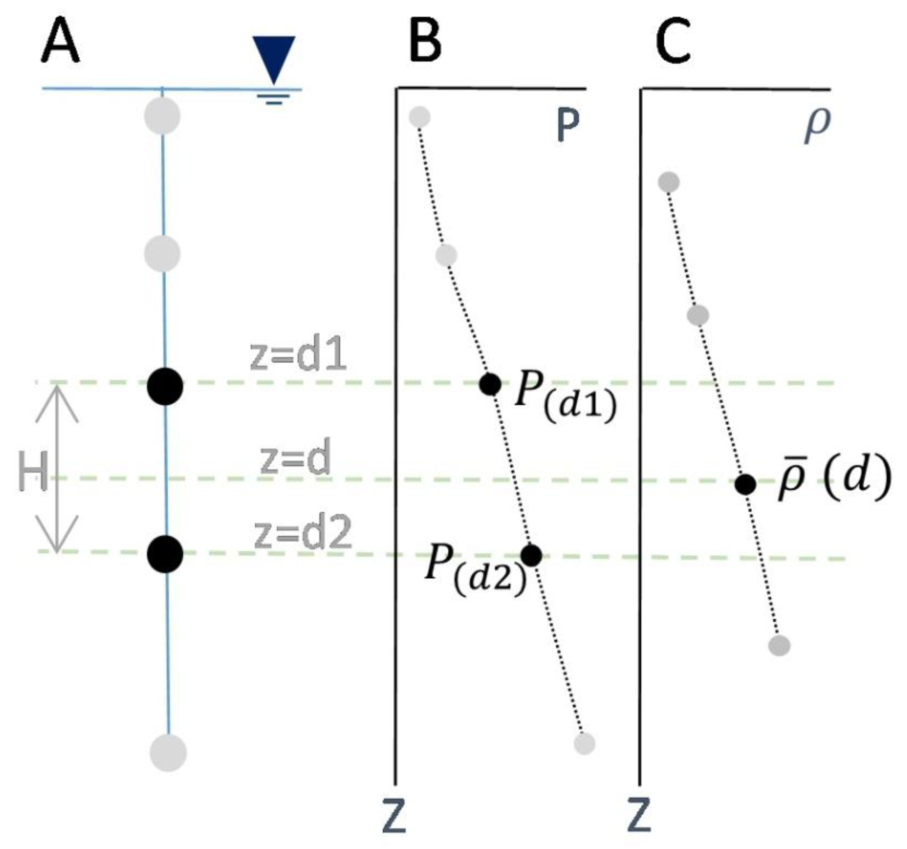
We resolved in situ density utilizing pressure sensors and hydrostatic relations as described below (see Figure 1 for notation and setup). The measured pressure at depth z (Figure 1B) is the sum of the atmospheric pressure ($P_{atm}$), the hydrostatic pressure ($P_{hyd }$), and the dynamic stress ($\sigma$).

$$P\left(z\right)=P_{atm}+P_{hyd}\left(z\right)+\sigma \left(z\right).$$

(1)

The hydrostatic pressure in the water column is determined as

$$P_{hyd}\left(z\right)={{\displaystyle \int }}_0^Z\rho \left(z\right)gdz,$$

(2)

where g is the acceleration due to gravity, and $\rho \left(z\right)$ is the water density along the water column (at water surface, z = 0). The pressure difference between two vertically separated sensors located at depths d1 and d2 (Figure 1A), eliminating the atmospheric pressure and the contribution of hydrostatic pressure above d1, is expressed as

$$\Delta P\left(z=d\right)=P_{ }\left(z=d2\right)-P_{ }\left(z=d1\right)=g{{\displaystyle \int }}_{d1}^{d2}\rho \left(z\right)dz+\delta \sigma ,$$

(3)

where $\delta \sigma$ is the difference in the dynamic stresses between d1 and d2. The average density, $\overline{\rho },$ at depth z = d, between d2 and d1 (Figure 1A), is expressed as

$$\overline{\rho }\left(z=d\right)=\frac{1}{d2-d1}{{\displaystyle \int }}_{d1}^{d2}\rho \left(z\right)dz.$$

(4)

If the dynamic stresses at d1 and d2 are similar and/or small compared to the hydrostatic pressure, i.e., $\delta \sigma \ll g{{\displaystyle \int }}_{d1}^{d2}\rho \left(z\right)dz$, then Equations (3) and (4) yield

$$\Delta P_{ }\left(z=d\right)\cong \overline{\rho }\left(z=d\right)·g·H,$$

(5)

where H = d2 − d1, and z = d is between d1 and d2. Thus, the average density at depth z = d is given below (Figure 1C).

$$\overline{\rho }\left(z=d\right)=\frac{ \Delta P_{ }\left(z=d\right)}{g·H}$$

(6)

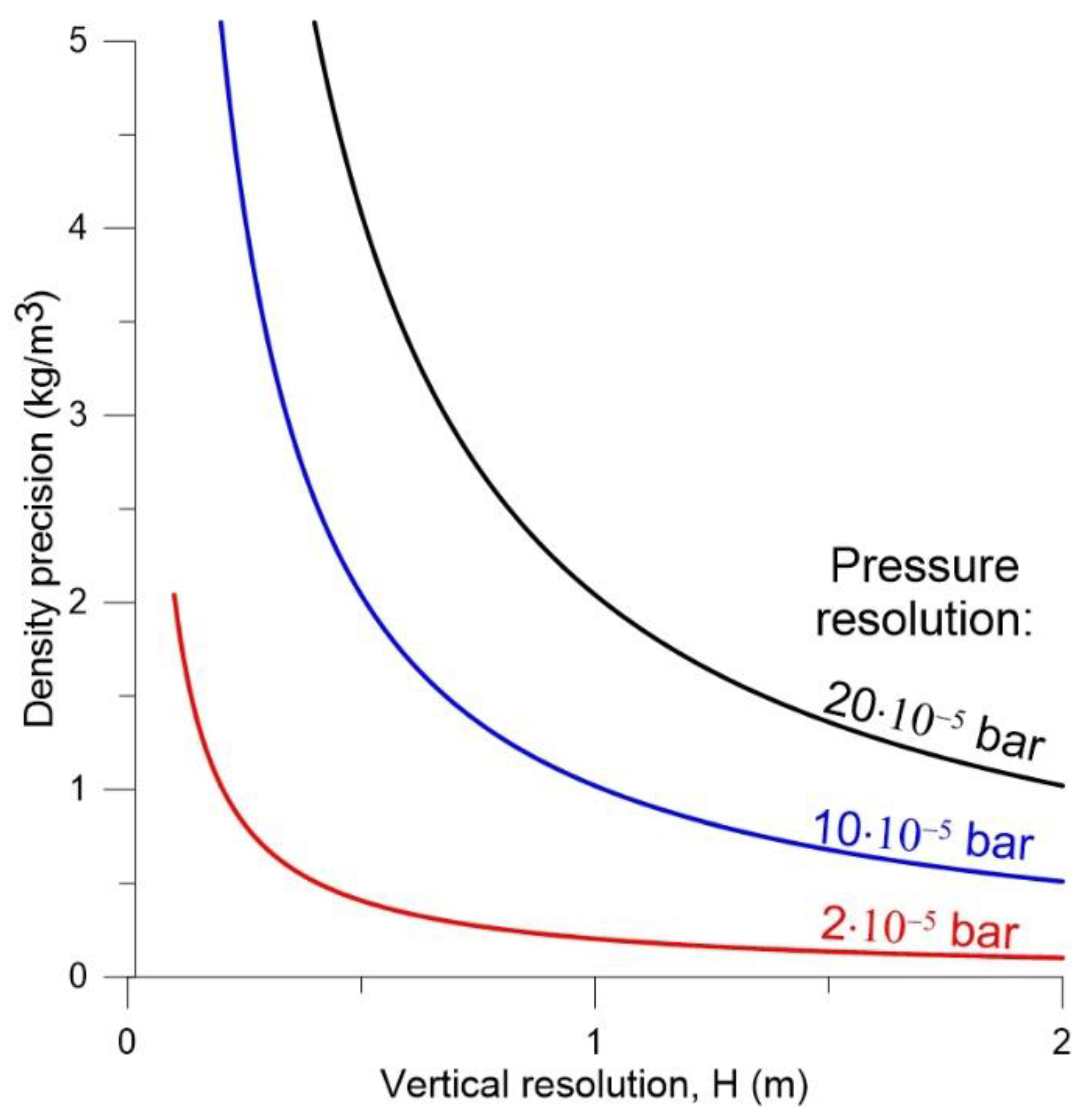
The precision of the density measurement, $\delta \overline{\rho }\left(z=d\right)$, depends on the resolution of the pressure measurement and on the vertical distance between the sensors, H (and on the value of g at the site). For a given pressure-sensor resolution ($\delta \Delta P)$, the density precision is expressed as

$$\overline{\rho }\left(z=d\right)+\delta \overline{\rho }\left(z=d\right)=\frac{ \Delta P_{ }\left(z=d\right)+\delta \Delta P}{g·H}.$$

(7)

Thus, there is an inverse relationship between the density precision and the vertical distance resolution (Figure 2).

$$\delta \overline{\rho }\left(z=d\right)\cong \frac{\delta \Delta P}{g·H}.$$

(8)

3. Methods

3.1. Density Measurements Using the Hydrostatic Densitometer

To explore the vertical distribution of the water density in a selected location, one needs to determine the vertical position and the number of sensors in the hydrostatic densitometer (Figure 1A and Figure 2, Equation (8)). We used an array of series 36XiW PAA 0.8–2.3 bar pressure (and temperature) transducers (Keller, Winterthur, Switzerland). The pressure accuracy of the transducers is 1.15 × 10⁻³ bar (corresponding to 0.05% of full scale, 2.3 bar) and the temperature accuracy is 0.1 °C. The pressure resolution is 1.15 × 10⁻⁵ bar (0.0005% of full scale) and the temperature resolution is 0.01 °C.

The natural environment is inherently noisy; therefore, to differentiate between background noise and the signal, one can perform measurements at a high frequency and carry out a statistical time-series analysis. We chose to measure at 10 Hz, which is the highest possible frequency for the measuring system used here, and we performed a 10 min average, which is the expected rate of environmental change. The data were recorded using a data logger (Model CR6, Campbell Scientific Inc., Logan, UT, USA).

3.2. Other Methods for Density Determination

To compare the density values from the hydrostatic densitometer, we measured density with the following commercial instruments: (i) an accurate laboratory density meter, oscillating U-tube, DMA 5000 (Anton Paar, Graz, Austria) with an accuracy of ±0.005 kg·m⁻³ (following [9,15,16]); (ii) a portable density meter, oscillating U-tube, DMA 35 (Anton Paar, Graz, Austria), with an accuracy of 1.0 kg·m⁻³; (iii) density measurements in the field, performed with a portable submersible density meter DM-250 (Lemis, Montgomery, TX, USA), with accuracy up to ±0.3 kg·m⁻³ and resolution of 0.1 kg·m⁻³.

4. Experimental Design and Regional Setting

4.1. Verification of the Hydrostatic Densitometer from Freshwater to Hypersaline Brine

As a preliminary step, before placing the hydrostatic densitometer system in the field, the system’s performance was examined in a set of controlled laboratory experiments. We tested the accuracy of the hydrostatic densitometer compared to commercial densitometers for water salinities ranging from Dead Sea brine (1242 kg·m⁻³) to distilled freshwater (996 kg·m⁻³). The pressure sensors were placed inside a specially designed aquarium to measure and examine all relevant pairs of sensors (i.e., the pairs that were placed in the field; see Section 4.3); five sensors were placed in the lower part of the aquarium, and five sensors were placed in the upper part, 1 m above (Figure 3A). We started the experiment with the saltiest brine (halite-saturated Dead Sea brine) and diluted it in 10 steps of ~25 kg·m⁻³ until distilled freshwater was obtained. Each segment of the experiment lasted ~15 min, following complete stirring and homogenization of the water in the aquarium, where pressure was measured at a rate of 10 Hz, i.e., ~10⁴ measurements per experimental step. For each water-dilution segment, (i) water was removed from the aquarium by a pump that sucked water from the bottom of the aquarium, (ii) distilled water was added to the aquarium bottom through a pipe, (iii) the water was mixed using the pump sucking water from the bottom and feeding it to the top to homogenize the brine, and (iv) the density of the brine was measured independently with the DMA 35 portable density meter, from both the bottom and top of the aquarium, to verify that homogeneity was achieved and for comparison with the hydrostatic densitometry approach. The experiment was performed on 24 May 2020.

4.2. Sensitivity of the Hydrostatic Densitometer to Variations in Temperature and Pressure

We tested the sensitivity of the hydrostatic densitometer to variations in pressure and temperature. The tested range of temperature variations was that expected at the field sites (25–34 °C), and the tested pressure variations were up to a water depth of ~10 m (the maximum height of the experimental device). These tests enabled us to determine the vertical position of the sensors in the best overall performers, i.e., to choose the optimal sensor couples along the array of sensors from all possible couples.

For the pressure-sensitivity test, the 10 pressure sensors (36XiW) were placed at the bottom of a 10 m column (Figure 3B). Water was filled to the top and was removed to ~1 m intervals (0.1 bar), from 2.0 bar to 0.9 bar. The experiment was performed on 6 July 2020.

For the temperature-sensitivity test, the 10 sensors were placed in a plastic pail filled with freshwater, inside a shaker incubator with controlled temperature (Qmax4000, Thermo Fisher, Waltham, MA, USA) (Figure 3C). The temperature was varied from 25 °C to 34 °C at 1 °C intervals (Figure 3C), and each interval was held for a few hours to achieve thermal equilibrium. The experiment was performed from 11–13 May 2020.

4.3. Field Campaign Design and Regional Setting

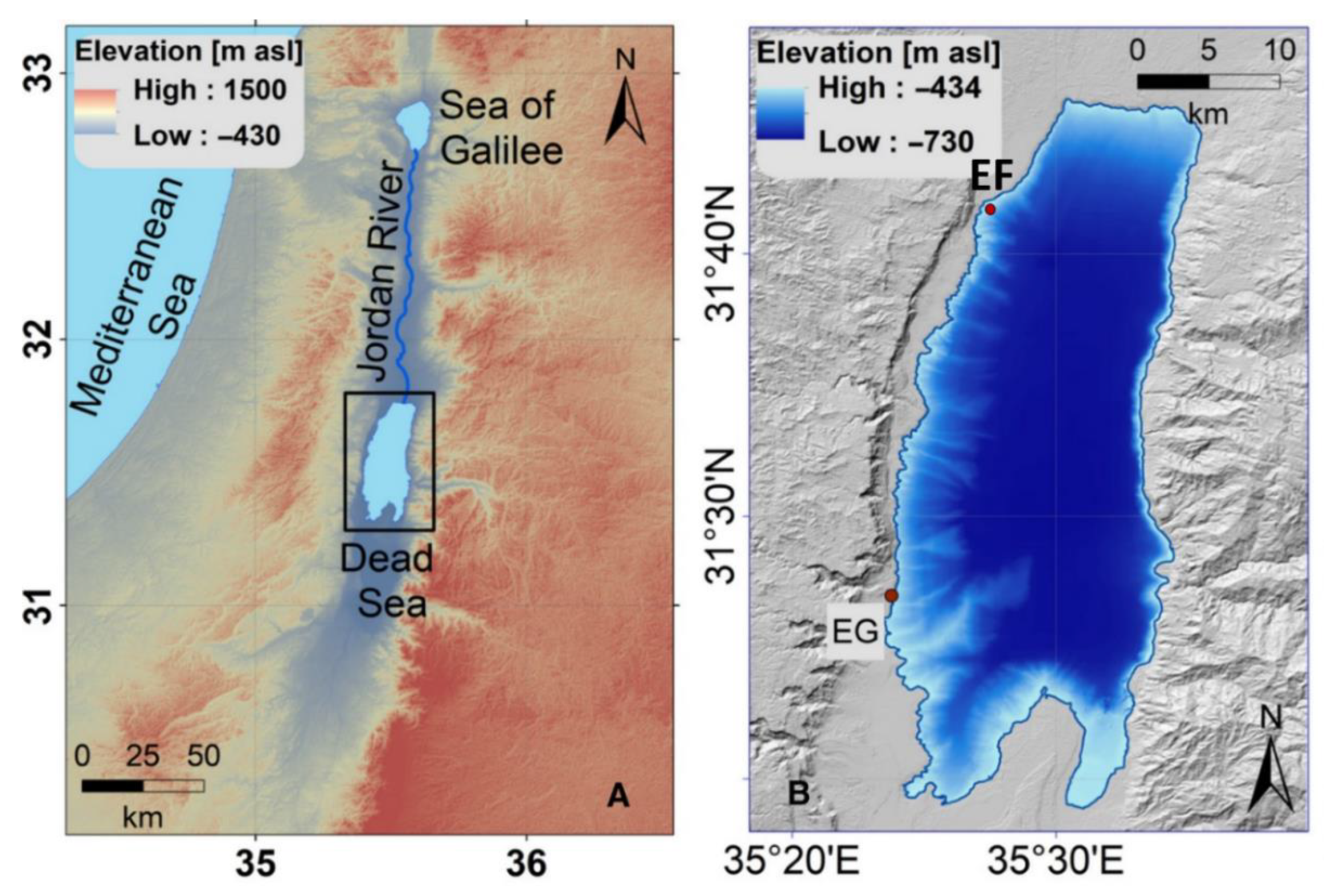
Our field campaigns were conducted at a buoy in the Dead Sea and in a borehole in the Dead Sea coastal aquifer. The Dead Sea is a hypersaline terminal lake located on the lowest land surface on Earth (Figure A1, Appendix A) which, in the last decade, has experienced a decline in lake level at a rate of ~1 m·year⁻¹ [19,20]. The Dead Sea salinity and density are 340 g·L⁻¹ and 1242 kg·m⁻³, respectively.

4.3.1. The Borehole Measuring Setup

The field campaign in the Dead Sea coastal aquifer was conducted where significant changes are expected to occur within a short time because of the rapid drop of the Dead Sea’s lake level. The Dead Sea and the adjoining groundwater system are hydraulically interconnected, as reflected by the relatively rapid (a few days) groundwater level response to level changes of the Dead Sea [21]. The fresh–saline water interface also responds to the drop in the lake’s level and the eastward shift of the Dead Sea shoreline, resulting in rapid flushing of the Dead Sea coastal aquifer [22].

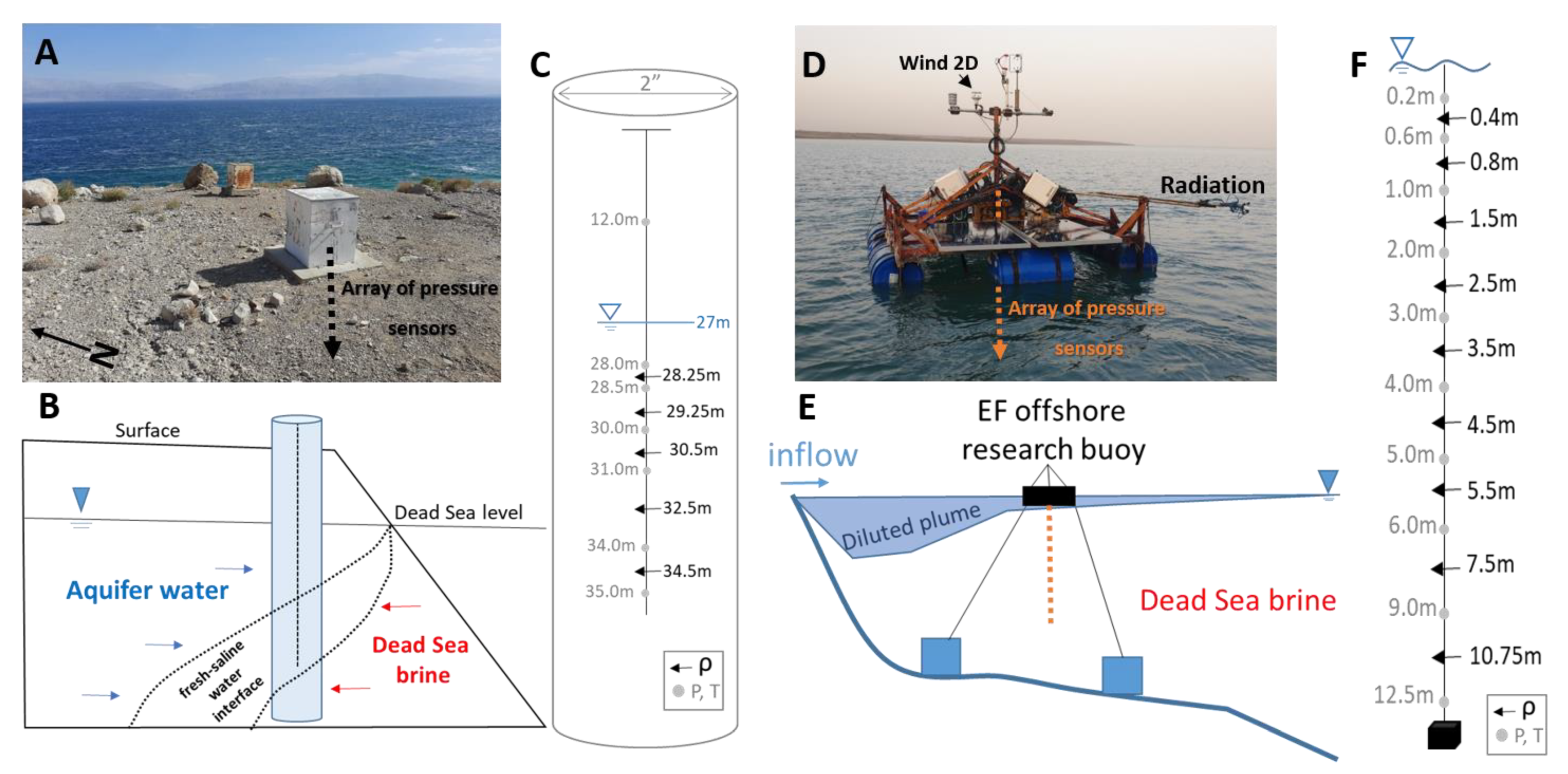
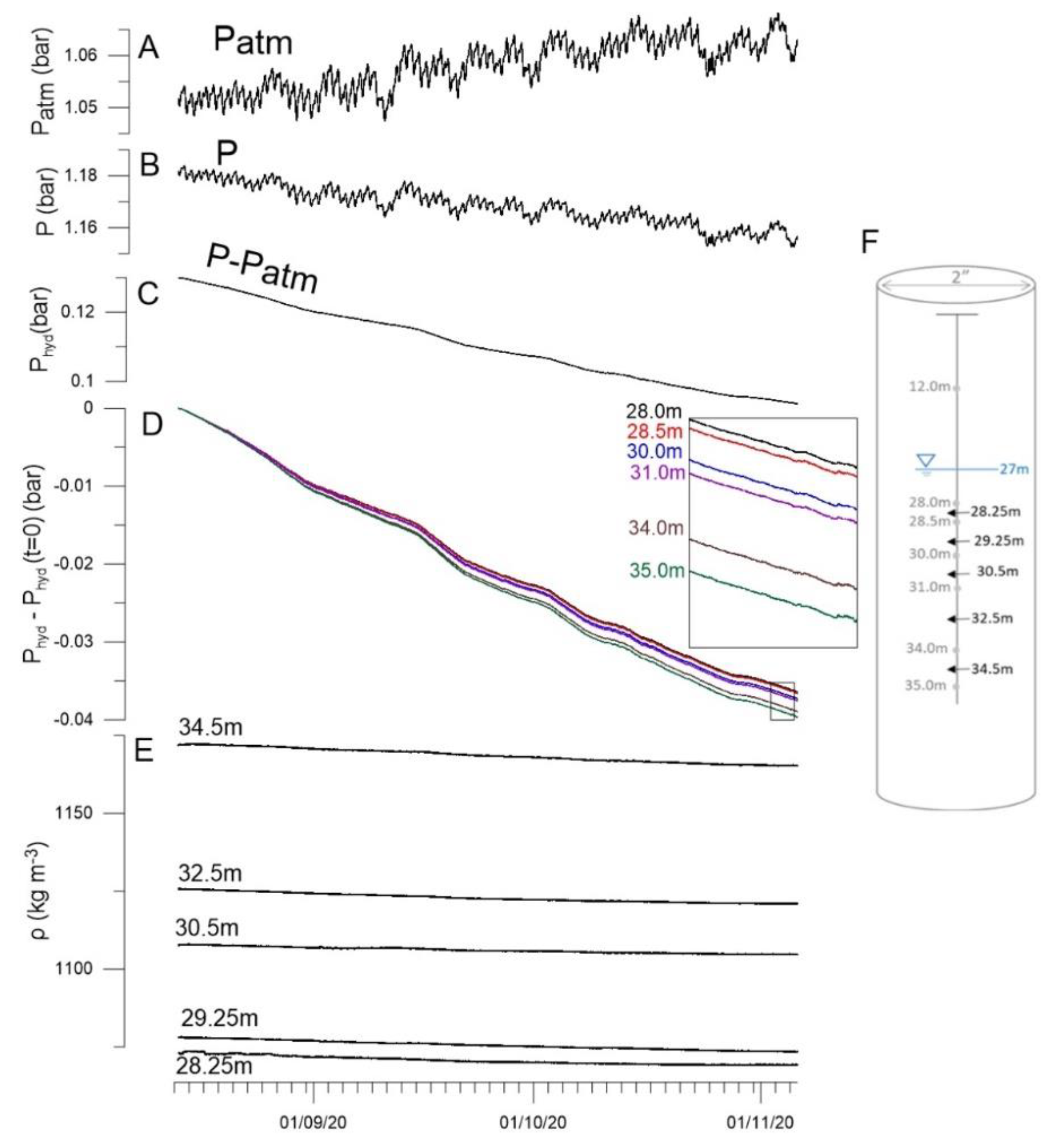
The array of pressure sensors was installed in the EG26 borehole (2” diameter pipe) (Figure 4A–C) for 84 days, from 13 August to 5 November 2020. EG26 is currently (2021) located ~70 m from the Dead Sea shoreline. Following Equation (8) and our prior knowledge of the vertical structure of the borehole water column [23], the hydrostatic densitometer sensors were placed at 28 m, 28.5 m, 30 m, 31 m, 34 m, and 35 m below the surface, along a water column of ~8 m (Figure 4C). The barometric pressure was measured at 12 m below the surface, inside the borehole. A water level of 26.69 m below the surface was measured before the system’s installation using a manual water level meter (model 101, Solinst, Georgetown, ON, Canada).

4.3.2. The Dead Sea Diluted Plume Measuring Setup

The second field campaign was conducted in the Dead Sea at the diluted plume fed by the Dead Sea’s largest spring, Ein Feshkha (EF, Figure A1, Appendix A), discharging around 70 × 10⁶ m³·year⁻¹ through a series of ~10 tributaries along ~1 km of shoreline [24]. These point sources of freshwater inflows form a diluted plume that spreads laterally over the Dead Sea [8]. The density difference between the inflowing freshwater and the Dead Sea brine is extreme, from 1.0 × 10³ kg·m⁻³ to 1.24 × 10³ kg·m⁻³. A schematic illustration of the EF diluted plume setup is shown in Figure 4E.

To measure the plume dynamics and heat fluxes from it, we installed a research buoy ~250 m offshore the spring outflow at the EF site (Figure 4D,E). The buoy is anchored with four concrete blocks (750 kg each) at 15 m water depth (Figure 4E). The buoy includes several sensors (above and in the water); here, we present data from the array of pressure sensors (Figure 4D–F), a two-dimensional sonic anemometer (WindSonic, Gill Instruments, Hampshire, UK), and a solar radiation sensor (CNR4, Kipp and Zonen B.V., Delft, The Netherlands) (Figure 4D).

The hydrostatic densitometer was installed on 3 February 2021. Following Equation (8) and our prior knowledge of the vertical structure of the diluted plume [8], the pressure sensors were located at water depths of 0.2 m, 0.6 m, 1 m, 2 m, 3 m, 4 m, 5 m, 6 m, 9 m, and 12.5 m; accordingly, the hydrostatic densitometer took measurements at water depths of 0.4 m, 0.8 m, 1.5 m, 2.5 m, 3.5 m, 4.5 m, 5.5 m, 7.5 m, and 10.7 m (Figure 4F).

5. Results and Discussion

5.1. Laboratory Experiment and Sensitivity Tests

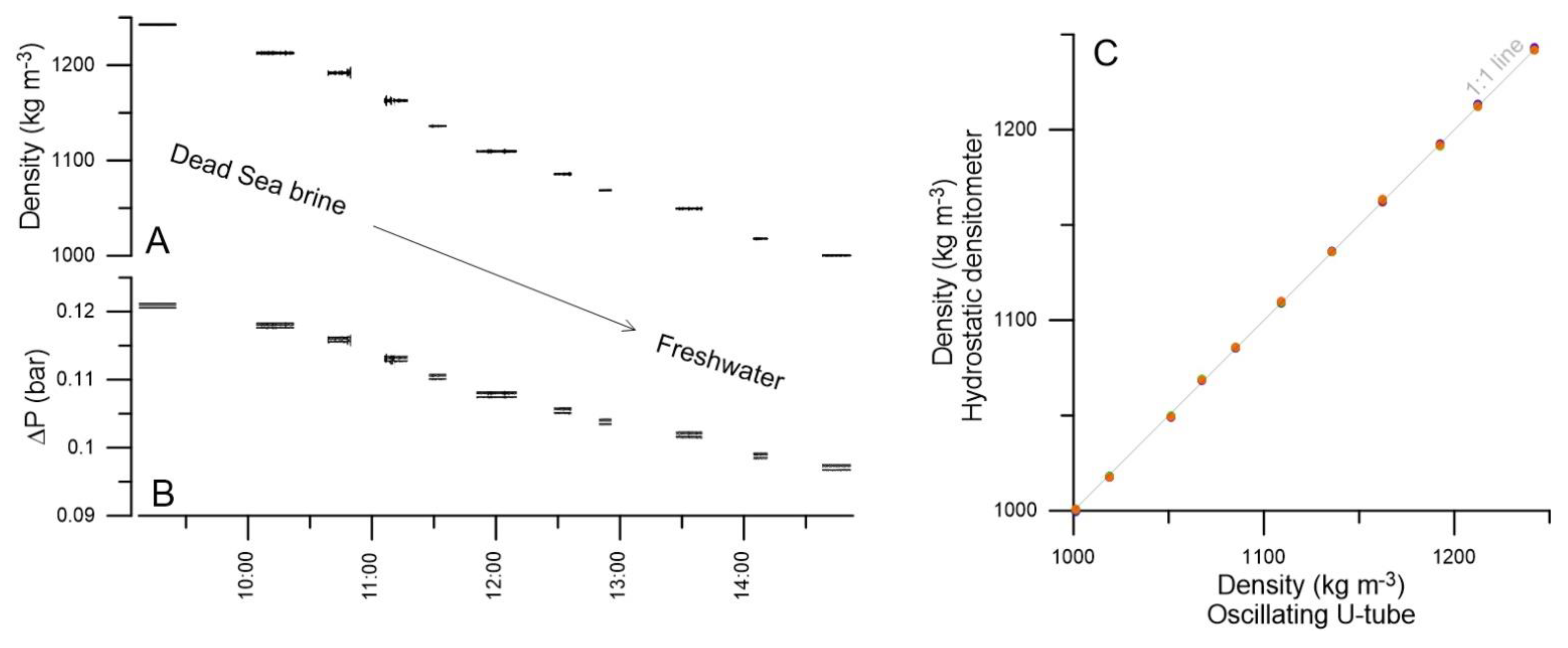
The performance of the hydrostatic densitometer (Equation (6)) was demonstrated in the laboratory using a set of nine pairs of pressure sensors (i.e., the pairs that were placed in the field; see Section 4.3) produced by two groups of five sensors with a vertical separation of 1 m (Figure 3A). The hydrostatic pressure difference (Equation (5)) between the nine pairs throughout the entire experiment is presented in Figure 5B, and the density values, calculated from the pressure difference (Equation (6)), are shown in Figure 5A. The dilution steps are seen as a reduction in pressure difference and density with each successive experimental step (Figure 5A,B, respectively). Instrument noise in the pressure-difference measurements was twice the declared instrument’s resolution (up to ~3 × 10⁻⁵ bar) and was small compared to the signal due to dilution (~0.02 bar), which means that, in this range, the sensors are very precise. Similarly, the calculated density between the experimental steps was ~25 kg·m⁻³ and the noise was ~0.3 kg·m⁻³. The accuracy of the hydrostatic densitometer can be evaluated when comparing, for each of the experimental steps, the density based on hydrostatic pressure with the density measurement by the standard density meter (Figure 5C).

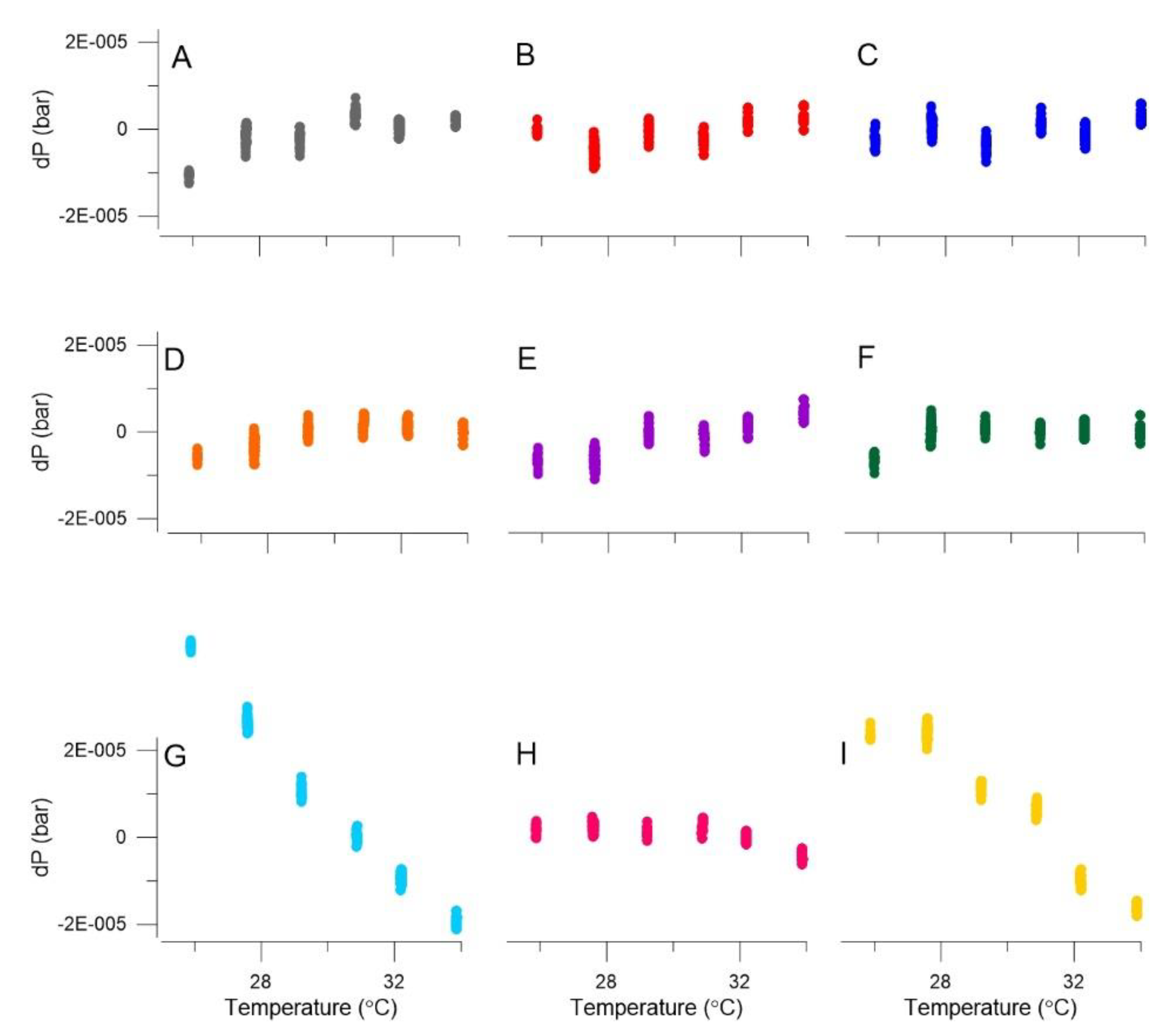
To evaluate the sensitivity of the hydrostatic densitometer (or the pressure difference) to variations in temperature and pressure in the deployment environment, we conducted sensitivity tests, presented in Figure A2 and Figure A3 (Appendix A), respectively. For a temperature range of 25–34 °C, the offset of the pressure differences between seven of the nine sensor pairs was within the declared resolution (less than ±2.3 × 10⁻⁵ bar) (Figure A2A–F,H, Appendix A); two pairs of sensors (Figure A2G,I, Appendix A) were within the declared accuracy (less than ±2.3 × 10⁻³ bar) and within 2–3 times the declared resolution (6 × 10⁻⁵ bar and 4.2 × 10⁻⁵ bar for 8 °C variations, Figure A2G,I, Appendix A, respectively). Therefore, the two pairs with higher sensitivity to temperature variations were located at water depths with relatively small temperature variations (i.e., 5.5 m and 10.7 m water depth in EF buoy, respectively; see Figure 4F).

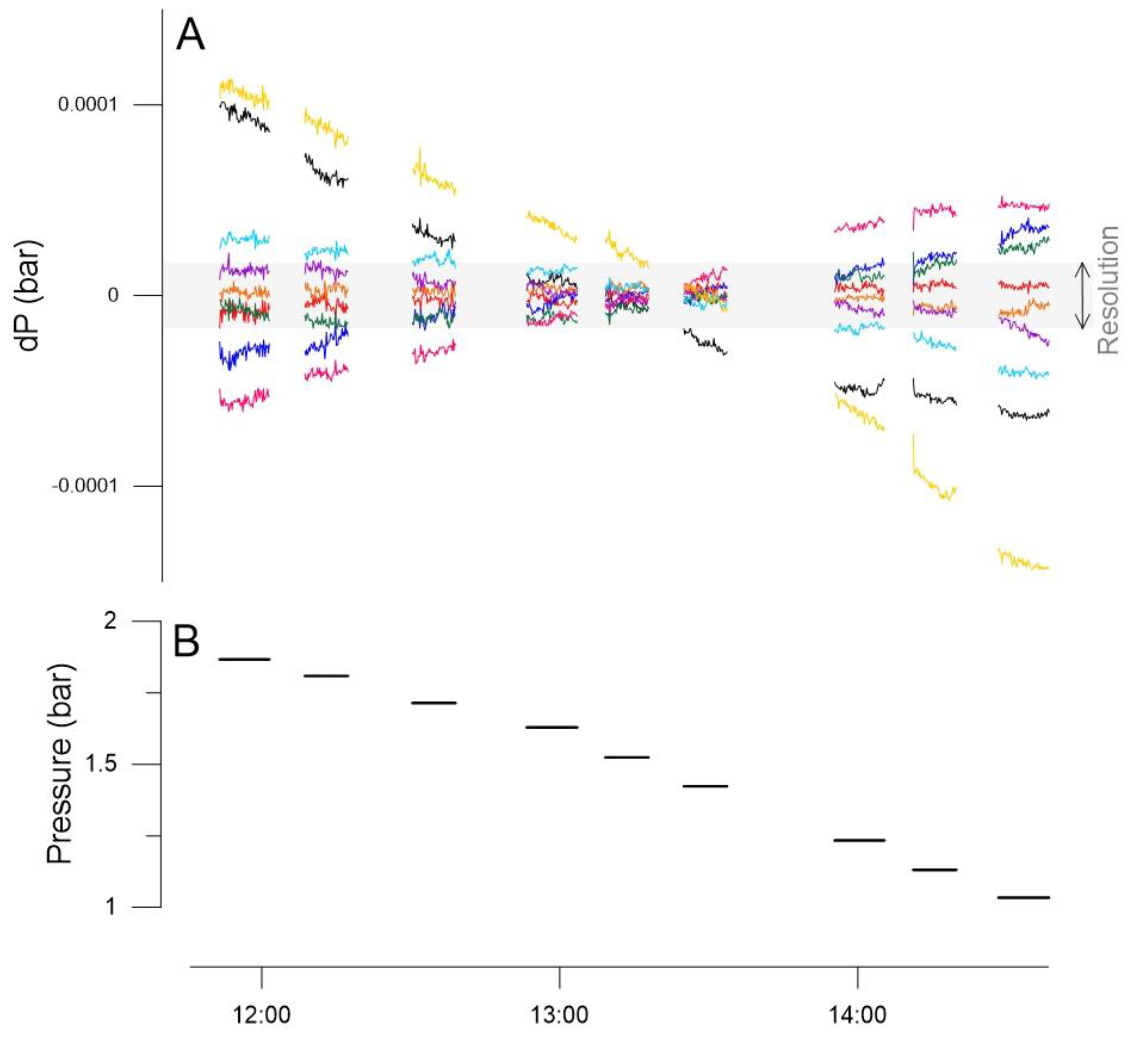
The sensitivity of the pressure difference to changing the pressure from ~1.8 bar to ~1.0 bar is presented in Figure A3A,B (Appendix A). The offset of the pressure difference ranges from ~2 × 10⁻⁵ bar to ~26 × 10⁻⁵ bar. Once the sensors are placed at a specific site in the field, one can overcome these sensitivities by calibrating the pressure differences and the hydrostatic density values with a standard density determination (using, e.g., the DMA 5000 densitometer) via sampling.

5.2. Coastal Aquifer—Borehole Stratification Observation

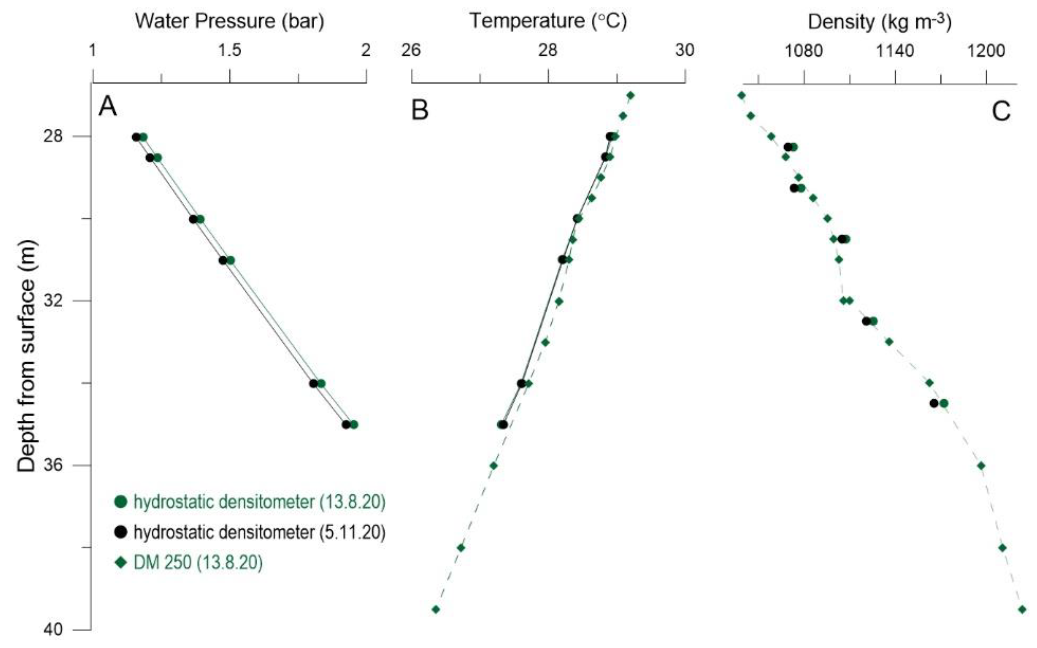
The vertical stratification of the borehole in the coastal aquifer at the Dead Sea shore (see setup in Section 4.3 and Figure 4) was documented continuously for 84 days by the hydrostatic densitometer deployed within a borehole. The atmospheric pressure (Figure 6A) was subtracted from the pressure measurement (Equation (1), Figure 6B), to compute the hydrostatic pressure values (Equation (2), Figure 6C). The time series of hydrostatic pressure (minus the initial pressure, P_hyd − P_hyd(t = 0)) of all sensors is shown in Figure 6D. The monotonic decrease in pressure in all sensors is due to the decline in groundwater level, following the decline in lake level (the sensors are fixed to the borehole top). The rate of pressure change varies with depth (insert in Figure 6D), with the deepest sensor showing the fastest rate of pressure decline. This means that the pressure difference between neighboring sensors increases with depth and with time. The density at different depths is presented in Figure 6E, based on Equation (6), showing that density increases with depth. The density at all depths decreases with time because the sensors are fixed at a particular depth; the groundwater table decreases with time, and fresher water approaches each pair of sensors. Moreover, the rate of freshening of the water column (rate of density decrease) increases with depth, reflecting widening of the freshwater–saline interface. Figure 7 presents the vertical profiles of pressure, temperature, and density at the beginning and end of the deployment. The temperature decreases with depth, at a gradient of ~0.2 °C·m⁻¹ (Figure 7B). The density increases with depth, from ~1070 kg·m⁻³ (at a water depth of ~1 m, ~28 m below the surface) to ~1224 kg·m⁻³ (water depth of ~13 m, ~40 m below the surface) (Figure 7C). The density profiles measured with two independent methods—the hydrostatic densitometer and the portable density meter (DM-250)—are similar. With time, the pressure measurements (Figure 7A) show a decrease in pressure at all depths measured as a result of a decrease in water level and a decrease in density due to dilution of the water column.

5.3. Lake Stratification—Diluted Plume Observation

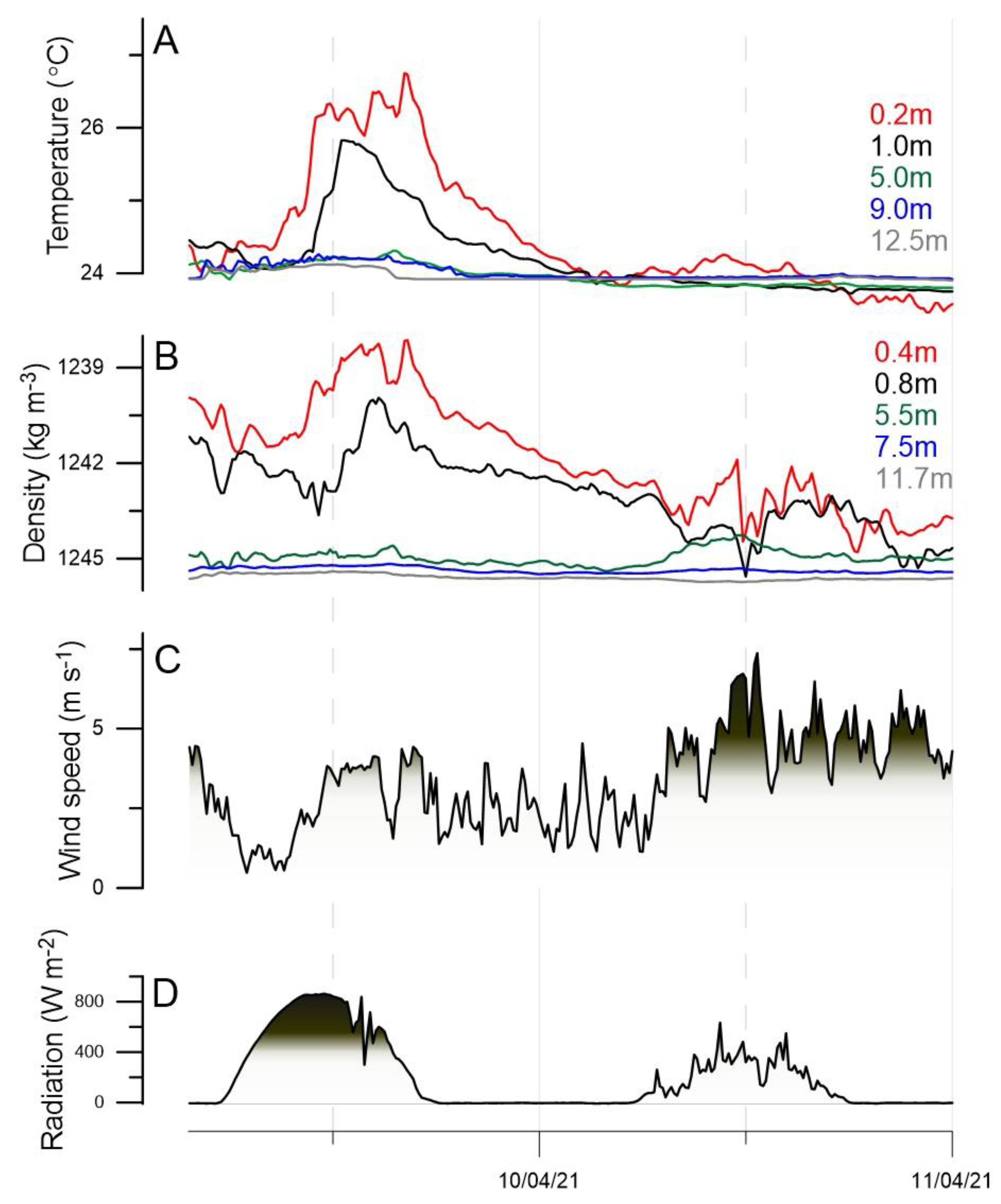
Data from the stratified diluted plume on two consecutive days are shown in Figure 8. The temperature and density measured at different depths are presented in Figure 8A,B, respectively, along with the atmospheric forcing, i.e., the wind speed and incoming solar radiation (Figure 8C,D, respectively). The temperature and density measurements show clear stratification, where the shallowest sensors (0.2 m and 0.4 m, respectively) exhibit the highest temporal variations, peaking during the afternoon with a temperature higher by 3 °C and density lower by 6 kg·m⁻³, respectively. The deepest sensors (12.5 m and 11.7 m, respectively) show almost constant values of temperature and density. The two observation days present opposing wind and radiation forcing. On the first day, the wind speed was low (<4 m·s⁻¹) and incoming radiation was high (~850 W·m⁻²), resulting in maximum thermal and density stratification at midday, with a difference between shallow and deep water of 3 °C and 6.5 kg·m⁻³. On the second day, the wind was strong (>5 m·s⁻¹), higher than the threshold for mixing by wind-waves [8,9,11,25,26,27], and clouds reduced the incoming radiation (~400 W·m⁻²), resulting in reduced stratification, i.e., depth stratification of 0.3 °C and <3 kg·m⁻³. With the intensification of wind speed (7:00 a.m. on 10 April), the density of the shallow water (0.4 m, 0.8 m) increased and, concurrently, the density of the deeper water (5.5 m) decreased, both because of wind-induced mixing. Note that the process of dilution, mixing, and daily heating is limited to the upper layers (<7 m).

Until now, we have been able to explore the continuous variations of stratification only via temperature variation [8,28], which lacks the variations in salinity and density stratification. This is the first documentation of continuous thermohaline stratification (density–depth and temperature–depth time series) in the Dead Sea or other hypersaline water bodies.

5.4. Challenges and Potential for Dynamic Marine Applications

When the hydrostatic densitometer is placed in a dynamic marine environment, the system design should maintain the array of pressure sensors upright; tilting (e.g., due to currents) will lead to changes in the vertical distance between the sensors and, thus, will result in lower calculated density. Possible ways of overcoming the tilting effect include using a large weight at the bottom of the device, or adding a tilt gauge to correct for the geometrical effect of the tilt, or both. Furthermore, it is possible to incorporate an additional pressure sensor in a standard CTD device, enabling measurement of hydrostatic density, in addition to other water properties, even in a hypersaline environment. This technique requires a way to isolate the hydrostatic pressure from the dynamic pressure following the lowering rate of the system, and to overcome the sensitivity to temperature and pressure variations by correcting the measured density.

The importance of measuring density in buoyant flows is key to predict the dynamics of dense gravity currents, where the density of the fluid is controlled by the suspended sediment load, in addition to salinity and temperature. Gravity flows are known for their importance as geofluids, as well as for their erosional capacity as coastal pipelines and infrastructures. Different buoyancies of the current lead to notable differences in the hydrodynamics (i.e., turbulent and mean velocities, bed shear stress, and turbulent stresses) and, consequently, to different processes of entrainment, transport, and deposition (e.g., [29,30]). The advantage of the hydrostatic densitometer is its ability to directly measure the fluid density and its variations with time and space and the fact that it does not require corrections of the concentration of suspended sediments.

6. Summary and Conclusions

The hydrostatic densitometer method allows, for the first time, continuous monitoring of density profiles over a wide range of water densities (salinities)—from freshwater to hypersaline brine. The method requires pressure sensors that are vertically separated to apply the hydrostatic relations between pressure differences and average density between the sensors; a chain of sensors provides continuous measuring of density (and temperature) along the water column.

We showed the applicability and accuracy of the hydrostatic densitometer in the laboratory, in a density range of 1–1.24 × 10³ kg·m⁻³, with a deviation of the hydrostatic densitometer measurements from the density measured with the standard acoustic densitometer of up to 1 kg·m⁻³ (R² = 0.99).

In the coastal borehole, we installed six sensors along a water column of ~8 m. We presented the level lowering measured by all pressure sensors, at a rate of ~0.01 bar month^-1, due to lowering of the Dead Sea level. The pressure differences between pairs of pressure sensors presented increasing density with depth, due to freshwater diluting the upper part of the aquifer over the hypersaline brine supplied by the lake. With time, density at all depths decreased at a rate of ~1.6 kg·m⁻³ per month, due to lowering of the upper diluted parts of the aquifer. The rate of density change increased with depth, reflecting widening of the freshwater–saline interface. The dynamics of the freshwater–saline interface associated with the rapid recession of the Dead Sea are documented here for the first time. Measurements of continuous changes in the width of the interface have never before been possible in such a saline environment.

At the diluted plume in the lake, we deployed a chain of 10 pressure (and temperature) sensors along the upper 13 m of the water column; the chain was attached to a buoy, thus keeping the sensors at the same depth relative to the lake surface. The density profile showed increasing density with depth, due to dilution by freshwater discharges from coastal springs. The temperature also varied, typically decreasing, with depth. With time, density and temperature stratification changed dramatically due to the changes in wind intensity and the resultant mixing, as well as due to changes in solar radiative forcing.

The design of a hydrostatic densitometer should account for the required depth and density resolution and the resolution of the pressure sensors. The highest resolution can be achieved by choosing the most accurate pressure sensor, from which the expected density resolution can be determined by choosing depth separation (Equation (8), Figure 2). Thus, optimal setup of the sensor chain depends on the nature of the stratification in the specific aquatic system.

We conclude that the hydrostatic densitometer method can be used to examine the dynamics of hypersaline environments which, until now, was limited by a lack of appropriate sensors.

References

- Bear, J. Dynamics of Fluids in Porous Media; Courier Corporation: Chelmsford, MA, USA, 2013; ISBN 0486131807. [Google Scholar]
- Knauss, J.A.; Garfield, N. Introduction to Physical Oceanography; Waveland Press: Long Grove, IL, USA, 2016; ISBN 1478634758. [Google Scholar]
- Werner, A.D.; Bakker, M.; Post, V.E.A.; Vandenbohede, A.; Lu, C.; Ataie-Ashtiani, B.; Simmons, C.T.; Barry, D.A. Seawater intrusion processes, investigation and management: Recent advances and future challenges. Adv. Water Resour. 2013, 51, 3–26. [Google Scholar] [CrossRef]
- Folch, A.; Menció, A.; Puig, R.; Soler, A.; Mas-Pla, J. Groundwater development effects on different scale hydrogeological systems using head, hydrochemical and isotopic data and implications for water resources management: The Selva basin (NE Spain). J. Hydrol. 2011, 403, 83–102. [Google Scholar] [CrossRef]
- Post, V.E.A.; von Asmuth, J.R. Review: Hydraulic head measurements—New technologies, classic pitfalls. Hydrogeol. J. 2013, 21, 737–750. [Google Scholar] [CrossRef] [Green Version]
- Levanon, E.; Yechieli, Y.; Shalev, E.; Friedman, V.; Gvirtzman, H. Reliable monitoring of the transition zone between fresh and saline waters in coastal aquifers. Groundw. Monit. Remediat. 2013, 33, 101–110. [Google Scholar] [CrossRef]
- Shalev, E.; Lazar, A.; Wollman, S.; Kington, S.; Yechieli, Y.; Gvirtzman, H. Biased monitoring of fresh water-salt water mixing zone in coastal aquifers. Groundwater 2009, 47, 49–56. [Google Scholar] [CrossRef]
- Mor, Z.; Assouline, S.; Tanny, J.; Lensky, I.M.; Lensky, N.G. Effect of Water Surface Salinity on Evaporation: The Case of a Diluted Buoyant Plume Over the Dead Sea. Water Resour. Res. 2018, 54, 1460–1475. [Google Scholar] [CrossRef]
- Arnon, A.; Lensky, N.G.; Selker, J.S. High resolution temperature sensing in the Dead Sea using fiber optics. Water Resour. Res. 2014, 50, 1756–1772. [Google Scholar] [CrossRef]
- Arnon, A.; Selker, J.S.; Lensky, N.G. Thermohaline stratification and double diffusion diapycnal fluxes in the hypersaline Dead Sea. Limnol. Oceanogr. 2016, 61, 1214–1231. [Google Scholar] [CrossRef]
- Arnon, A.; Brenner, S.; Selker, J.S.; Gertman, I.; Lensky, N.G. Seasonal dynamics of internal waves governed by stratification stability and wind: Analysis of high-resolution observations from the Dead Sea. Limnol. Oceanogr. 2019, 64, 1864–1882. [Google Scholar] [CrossRef]
- Sirota, I.; Enzel, Y.; Lensky, N.G. Temperature seasonality control on modern halite layers in the Dead Sea: In situ observations. Bull. Geol. Soc. Am. 2017, 129, 1181–1194. [Google Scholar] [CrossRef]
- Anati, D.A. The salinity of hypersaline brines: Concepts and misconceptions. Int. J. Salt Lake Res. 1999, 8, 55–70. [Google Scholar] [CrossRef]
- Sirota, I.; Arnon, A.; Lensky, N.G. Seasonal variations of halite saturation in the Dead Sea. Water Resour. Res. 2016, 52, 7151–7162. [Google Scholar] [CrossRef]
- Gertman, I.; Hecht, A. The Dead Sea hydrography from 1992 to 2000. J. Mar. Syst. 2002, 35, 169–181. [Google Scholar] [CrossRef] [Green Version]
- Gertman, I.; Kress, N.; Katsenelson, B.; Zavialov, P. Equations of State for the Dead Sea and Aral Sea: Searching for Common Approaches; Report IOLR/12; Israel Oceanographic and Limnological Research (IOLR): Haifa, Israel, 2010. [Google Scholar]
- Selker, J.S.; Thevenaz, L.; Huwald, H.; Mallet, A.; Luxemburg, W.; Van De Giesen, N.; Stejskal, M.; Zeman, J.; Westhoff, M.; Parlange, M.B. Distributed fiber-optic temperature sensing for hydrologic systems. Water Resour. Res. 2006, 42. [Google Scholar] [CrossRef] [Green Version]
- Lipták, B.G. Instrument Engineers’ Handbook, Volume One: Process Measurement and Analysis; CRC Press: Boca Raton, FL, USA, 2003; Volume 1, ISBN 1420064029. [Google Scholar]
- Lensky, N.G.; Dvorkin, Y.; Lyakhovsky, V.; Gertman, I.; Gavrieli, I. Water, salt, and energy balances of the Dead Sea. Water Resour. Res. 2005, 41. [Google Scholar] [CrossRef]
- Lensky, N.; Dente, E. The Hydrological Processes Driving the Accelerated Dead Sea Level Decline in the Past Decades; Rep GSI/16/2015; Geological Survey of Israel: Jerusalem, Israel, 2015.
- Yechieli, Y.; Ronen, D.; Berkowitz, B.; Dershowitz, W.S.; Hadad, A. Aquifer characteristics derived from the interaction between water levels of a terminal lake (Dead Sea) and an adjacent aquifer. Water Resour. Res. 1995, 31, 893–902. [Google Scholar] [CrossRef]
- Kiro, Y.; Yechieli, Y.; Lyakhovsky, V.; Shalev, E.; Starinsky, A. Time response of the water table and saltwater transition zone to a base level drop. Water Resour. Res. 2008, 44. [Google Scholar] [CrossRef] [Green Version]
- Yechieli, Y.; Sawaed, I.; Lutzky, H. Geological and Hydrological Findings from Boreholes at En Gedi, Hamme Mazor and Nahal Zeelim Area; Report TRGSI/14/2008; Geological Survey of Israel: Jerusalem, Israel, 2013. (In Hebrew)
- Dente, E.; Lensky, N.G.; Morin, E.; Enzel, Y. From straight to deeply incised meandering channels: Slope impact on sinuosity of confined streams. Earth Surf. Process. Landf. 2021, 46, 1041–1054. [Google Scholar] [CrossRef]
- Nehorai, R.; Lensky, I.M.; Lensky, N.G.; Shiff, S. Remote sensing of the Dead Sea surface temperature. J. Geophys. Res. 2009, 114, C05021. [Google Scholar] [CrossRef]
- Nehorai, R.; Lensky, I.M.; Hochman, L.; Gertman, I.; Brenner, S.; Muskin, A.; Lensky, N.G. Satellite observations of turbidity in the Dead Sea. J. Geophys. Res. Ocean 2013, 118, 3146–3160. [Google Scholar] [CrossRef]
- Nehorai, R.; Lensky, N.; Brenner, S.; Lensky, I. The dynamics of the skin temperature of the dead sea. Adv. Meteorol. 2013, 2013. [Google Scholar] [CrossRef]
- Sirota, I.; Ouillon, R.; Mor, Z.; Meiburg, E.; Enzel, Y.; Arnon, A.; Lensky, N.G. Hydroclimatic Controls on Salt Fluxes and Halite Deposition in the Dead Sea and the Shaping of “Salt Giants”. Geophys. Res. Lett. 2020, 47, e2020GL090836. [Google Scholar] [CrossRef]
- Meiburg, E.; Kneller, B. Turbidity currents and their deposits. Annu. Rev. Fluid Mech. 2010, 42, 135–156. [Google Scholar] [CrossRef] [Green Version]
- Zordan, J.; Juez, C.; Schleiss, A.J.; Franca, M.J. Entrainment, transport and deposition of sediment by saline gravity currents. Adv. Water Resour. 2018, 115, 17–32. [Google Scholar] [CrossRef]
Figure 1.
Schematic illustration of the setup of the hydrostatic densitometer. (A) Array of pressure sensors along a submerged vertical chain. The pressure sensors represented by black dots are located at z = d1 and z = d2 with a vertical separation of H; z = d is the midpoint between the sensors. (B) Pressure–depth profile; pressures at z = d1 and z = d2 are represented with black dots. (C) Density profile resolved from the pressure sensor and hydrostatic relations (Equations (4) and (6)). The average density (Equation (6)) at depth z = d is represented with a black dot.
Figure 2.
Resolution of the hydrostatic profiler based on Equation (8). The density precision and the vertical-distance resolution are anticorrelated, and the performance depends on the pressure sensor resolution. We present the solution of Equation (8) for three common pressure resolutions in typical pressure transducers. Using this diagram, one can examine the feasibility of using the hydrostatic densitometer for a specific system with a given density gradient.
Figure 3.
Laboratory experiment design. (A) Verification of the hydrostatic densitometer in water density ranging from freshwater (FW) to hypersaline brine (DS brine). The sensors were placed on a steel cage inside a water tank, in two groups of five with 1 m vertical separation. (B) Sensitivity of the hydrostatic densitometer to variations in pressure. The 10 sensors were placed at the bottom of a 10 m long column filled with freshwater. (C) Sensitivity of the hydrostatic densitometer to variations in temperature. The 10 sensors were placed in a pail of water inside a shaker incubator.
Figure 4.
(A) EG26 borehole. (B) Schematic illustration of EG26 borehole. (C) Schematic illustration of the hydrostatic densitometer in the EG26 borehole. (D) Ein Feshkha (EF) research buoy. (E) Schematic illustration of EF buoy and the diluted plume due to freshwater inflow into the Dead Sea. The hydrostatic densitometer is represented by a dotted orange line. (F) Schematic illustration of the hydrostatic densitometer at the EF buoy.
Figure 5.
The hydrostatic densitometer laboratory experiment. The experiment lasted 6 h (24 May 2020), including 11 steps of water dilution from Dead Sea brine to distilled freshwater; the period of water mixing is excluded. The measured density and pressure difference for the nine pairs of pressure sensors presented in (A) and (B), respectively. (C) Measured density from the hydrostatic densitometer vs. the DMA 35 oscillating U-tube densitometer; the accuracy of the hydrostatic densitometer is confirmed by the close fit to the standard density measurement (1:1 line) with an R2 value of 0.99.
Figure 6.
Temporal variations of the vertical properties at the coastal aquifer. (A) Atmospheric pressure. (B) Water pressure (Equation (1)) of 28 m sensor. (C) Hydrostatic pressure (Equation (3)) at the 28 m sensor (assuming negligible dynamic pressure). (D) Hydrostatic pressure at all depths, relative to initial values (Phyd − Phyd (t = 0)). The insert includes the depth of the sensors. (E) Density variation with time at different depths based on the hydrostatic densitometer (Equation (6)). (F) Schematic illustration of the hydrostatic densitometer in the EG26 borehole (see Section 4 for more details).
Figure 7.
The borehole water profiles. Measured scalars along the borehole: (A) water pressure; (B) temperature; (C) density. The profiles were measured at the beginning and end of the deployment (dates in dd.mm.yy). The density profiles were measured with two independent methods: the hydrostatic densitometer and the portable density meter, showing good agreement (see text).
Figure 8.
Time series of the stratification of the diluted plume. Temperature (A) and density (B) variations with depth. Atmospheric forcing: wind speed (C) and solar radiation (D). Wind speed above 4 m·s−1 is highlighted, as this is the threshold for wind-wave mixing.
Publisher’s Note: MDPI stays neutral with regard to jurisdictional claims in published maps and institutional affiliations. |
© 2021 by the authors. Licensee MDPI, Basel, Switzerland. This article is an open access article distributed under the terms and conditions of the Creative Commons Attribution (CC BY) license (https://creativecommons.org/licenses/by/4.0/).
Share and Cite
MDPI and ACS Style
Mor, Z.; Lutzky, H.; Shalev, E.; Lensky, N.G. Hydrostatic Densitometer for Monitoring Density in Freshwater to Hypersaline Water Bodies. Water 2021, 13, 1842. https://doi.org/10.3390/w13131842
AMA Style
Mor Z, Lutzky H, Shalev E, Lensky NG. Hydrostatic Densitometer for Monitoring Density in Freshwater to Hypersaline Water Bodies. Water. 2021; 13(13):1842. https://doi.org/10.3390/w13131842
Chicago/Turabian StyleMor, Ziv, Hallel Lutzky, Eyal Shalev, and Nadav G. Lensky. 2021. "Hydrostatic Densitometer for Monitoring Density in Freshwater to Hypersaline Water Bodies" Water 13, no. 13: 1842. https://doi.org/10.3390/w13131842
Note that from the first issue of 2016, this journal uses article numbers instead of page numbers. See further details here.