
Determining the Regional Geochemical Background for Dissolved Trace Metals and Metalloids in Stream Waters: Protocol, Results and Limitations—The Upper Loire River Basin (France)

 ,
,
Abstract
:1. Introduction
2. Regional Context
3. Methods
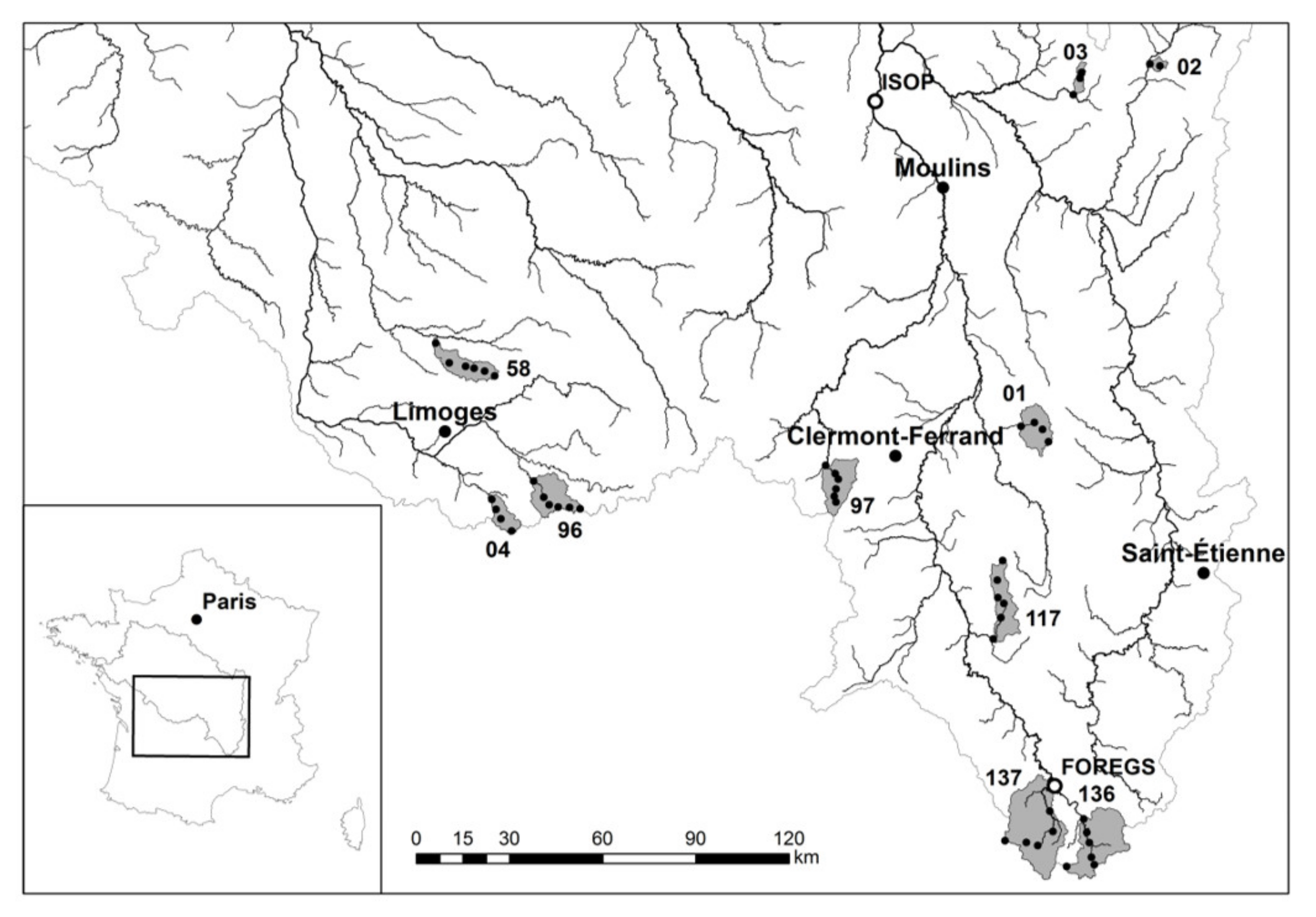
3.1. Watershed Selection
3.2. Materials and Methods
3.2.1. Sampling and Analytical Chemistry
3.2.2. Lead Stable Isotopes
3.2.3. Reaction Conditions
4. Results
4.1. Spring Sediments
4.2. Reaction Conditions
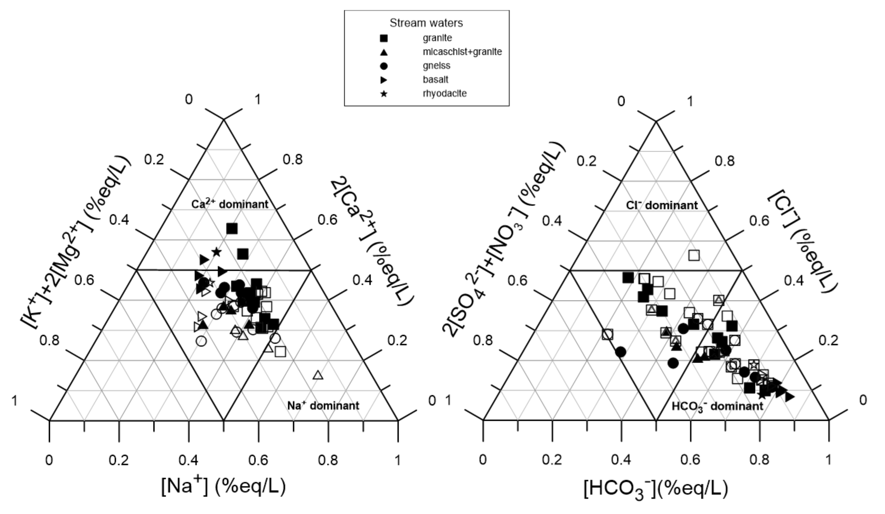
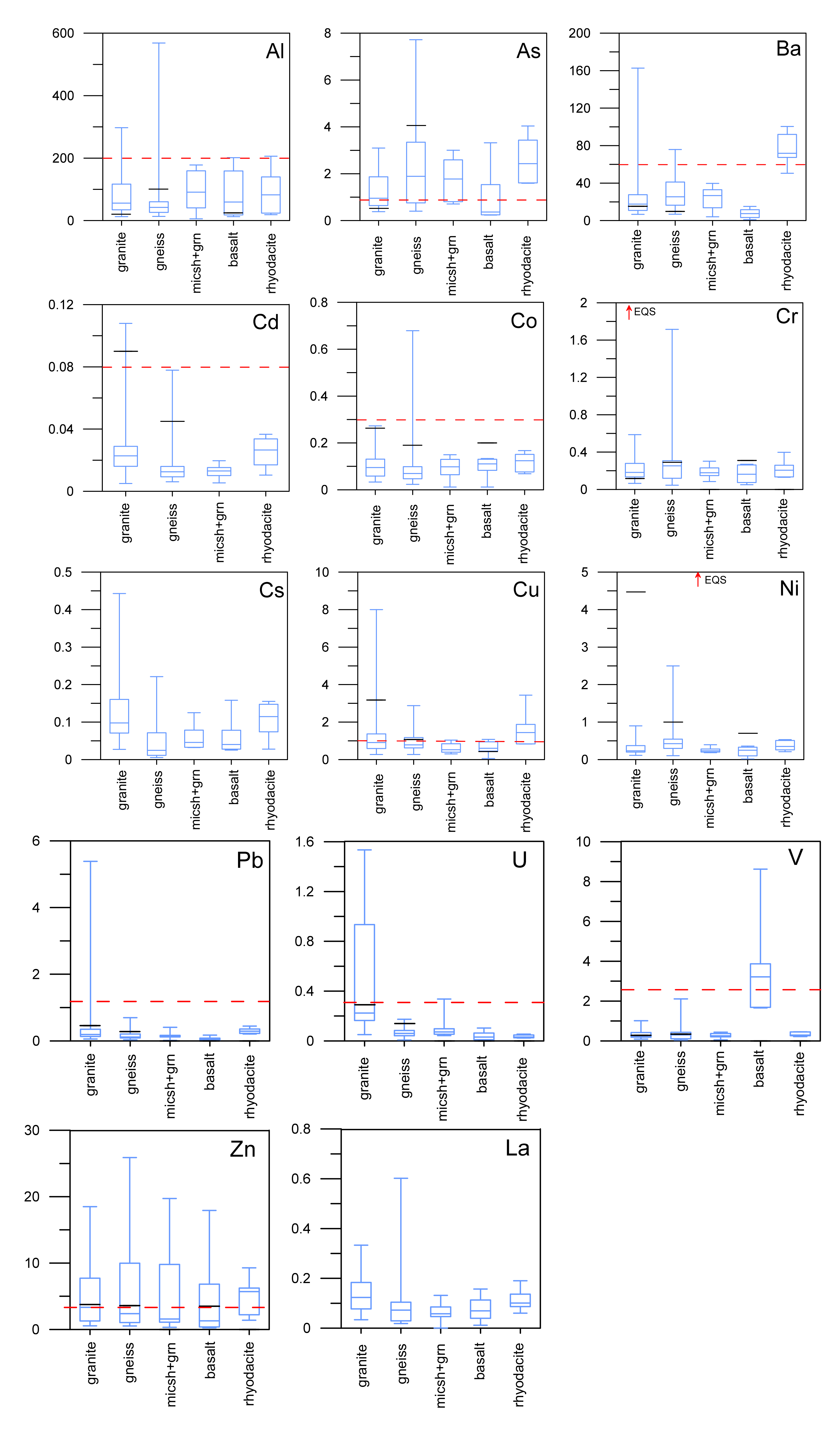
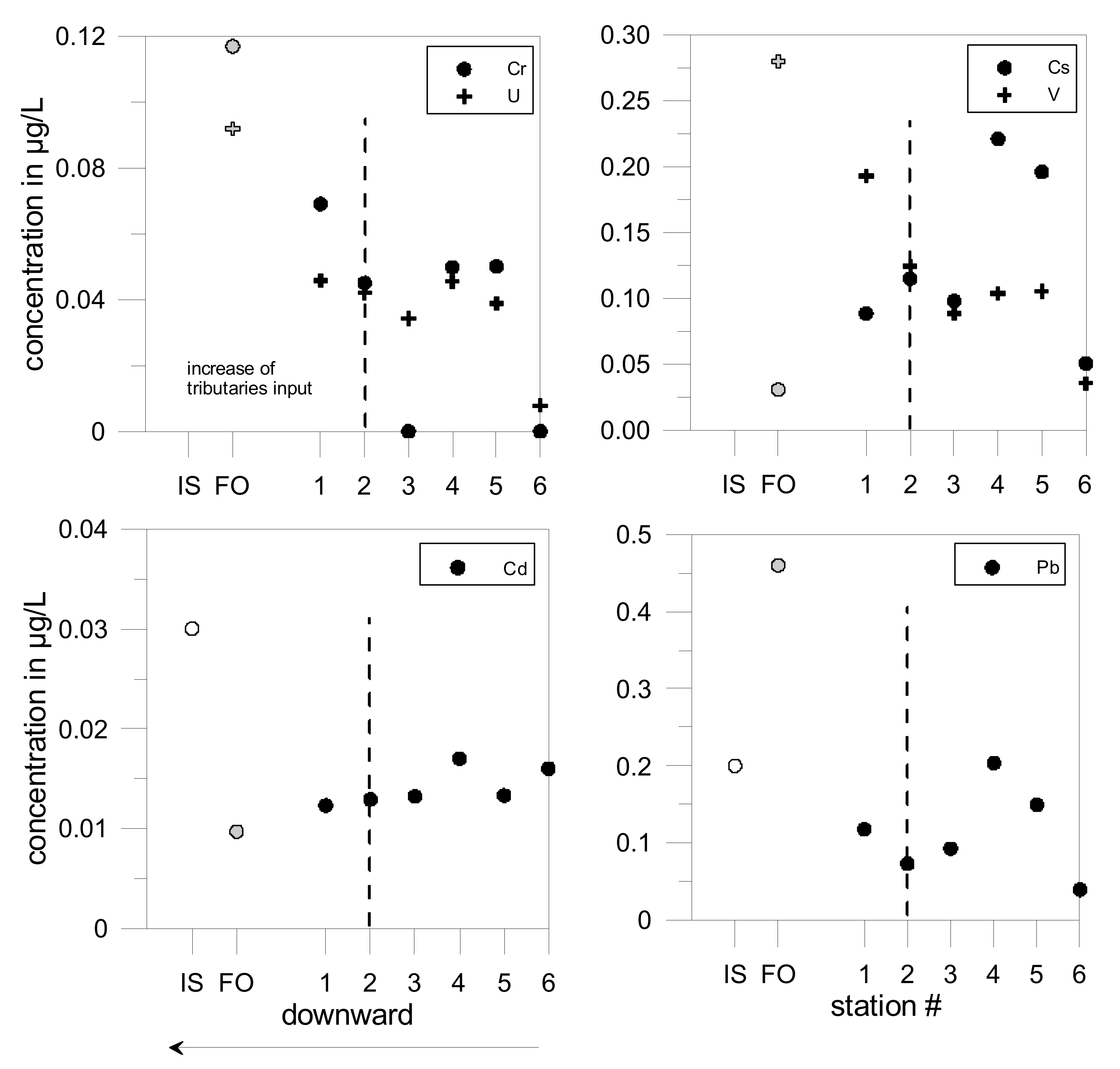
4.3. Dissolved Trace Metals and Metalloids
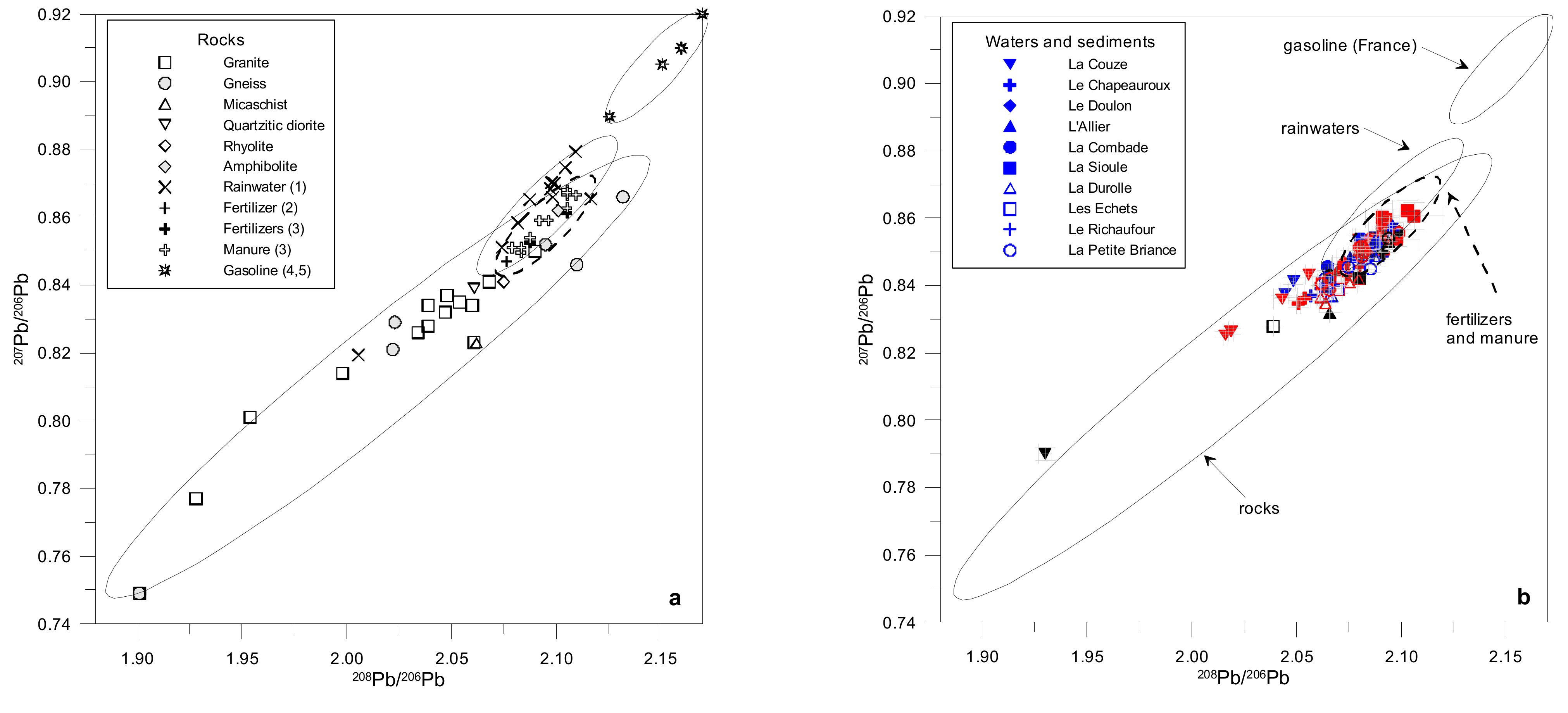
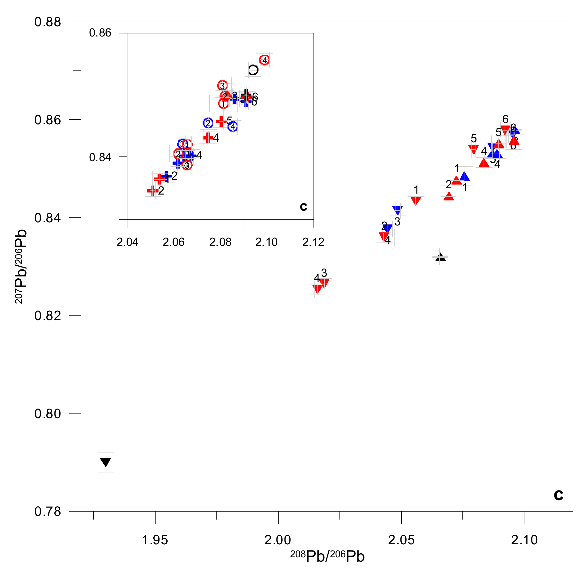
4.4. Lead Stable Isotopes
5. Discussion
5.1. Origin of TMM in Stream Waters
5.2. Trace Elements Geochemical Baseline
6. Conclusions
Supplementary Materials
Author Contributions
Funding
Institutional Review Board Statement
Informed Consent Statement
Data Availability Statement
Acknowledgments
Conflicts of Interest
References
- European Council. Directive of the European Parliament and of the Council (2000/60/EC) Establishing a Framework of Community Action in the Field of Water Policy; European Council: Brussels, Belgium, 2000. [Google Scholar]
- European Council. Directive of the European Parliament and of the Council of 12 August 2013 (2013/39/EC) Amending Directives 2000/60/EC and 2008/105/EC as Regards Priority Substances in the Field of Water Policy; European Council: Brussels, Belgium, 2013. [Google Scholar]
- Qu, S.; Wu, W.; Nel, W.; Ji, J. The behavior of metals/metalloids during natural weathering: A systematic study of the mono-lithological watersheds in the upper Pearl River Basin, China. Sci. Total Environ. 2020, 708, 134572. [Google Scholar] [CrossRef] [PubMed]
- Shaheen, S.M.; Rinklebe, J. Geochemical fractions of chromium, copper, and zinc and their vertical distribution in floodplain soil profiles along the Central Elbe River, Germany. Geoderma 2014, 228–229, 142–159. [Google Scholar] [CrossRef]
- Chapela Lara, M.; Buss, H.L.; Pogge von Strandmann, P.A.E.; Schuessler, J.A.; Moore, O.W. The influence of critical zone processes on the Mg isotope budget in a tropical, highly weathered andesitic catchment. Geochim. Cosmochim. Acta 2017, 202, 77–100. [Google Scholar] [CrossRef] [Green Version]
- Murozumi, M.; Chow, T.J.; Patterson, C.C. Chemical concentrations of pollutant lead aerosols, terrestrial dusts and sea-salts in Greenland and Antarctic snow strata. Geochim. Cosmochim. Acta 1969, 33, 1247–1294. [Google Scholar] [CrossRef]
- Steinnes, E.; Friedland, A.J. Metal contamination of natural surface soils from long range atmospheric transport: Existing and missing knowledge. Environ. Rev. 2006, 14, 169–186. [Google Scholar] [CrossRef]
- Cong, Z.Y.; Kang, S.C.; Zhang, Y.; Gao, S.; Wang, Z.; Liu, B.; Wan, X. New insights into trace element wet deposition in the Himalayas: Amounts, seasonal patterns, and implications. Environ. Sci. Pollut. Res. 2015, 22, 2735–2744. [Google Scholar] [CrossRef] [PubMed]
- Bing, H.; Wu, Y.; Li, J.; Xiang, Z.; Luo, X.; Zhou, J.; Sun, H.; Zhang, G. Biomonitoring trace element contamination impacted by atmospheric deposition in China’s remote mountains. Atmos. Res. 2019, 224, 30–41. [Google Scholar] [CrossRef]
- Salminen, R.; Gregorauskiene, V. Considerations regarding the definition of a geochemical baseline of elements in the surficial materials in areas differing in basic geology. Appl. Geochem. 2000, 15, 647–653. [Google Scholar] [CrossRef]
- Reimann, C.; Garrett, R.G. Geochemical background—concept and reality. Sci. Total Environ. 2005, 350, 12–27. [Google Scholar] [CrossRef] [PubMed]
- Johnson, C.C.; Breward, N. G-BASE Geochemical Baseline Survey of the Environment., Commissioned Report, CR/04/016N; British Geological Survey: Nottinghamshire, UK, 2004. [Google Scholar]
- Salminen, R.; Batista, M.J.; Bidovec, M. Geochemical Atlas of Europe, Part 1 Geological Survey of Finland Publication. 2006. Available online: www.gtk.fi/publ/foregsatlas (accessed on 26 June 2021).
- Albanese, S.; De Vivo, B.; Lima, A.; Cicchella, D. Geochemical background and baseline values of toxic elements in stream sediments of Campania region (Italy). J. Geochem. Explor. 2007, 93, 21–34. [Google Scholar] [CrossRef]
- Larrose, A.; Coynel, A.; Schäfer, J.; Blanc, G.; Massé, L.; Maneux, E. Assessing the current state of the Gironde Estuary by mapping priority contaminant distribution and risk potential in surface sediment. Appl. Geochem. 2010, 25, 1912–1923. [Google Scholar] [CrossRef]
- Imrie, C.E.; Korre, A.; Munoz-Melendez, G.; Thornton, I.; Durucan, S. Application of factorial kriging analysis to the FOREGS European topsoil geochemistry database. Sci. Total. Environ. 2008, 393, 96–110. [Google Scholar] [CrossRef]
- Reimann, C.; Fabian, K.; Birke, M.; Filzmoser, P.; Demetriades, A.; Négrel, P.; Oorts, K.; Matschullat, J.; de Caritat, P.; Albanese, S.; et al. GEMAS: Establishing geochemical background and threshold for 53 chemical elements in European agricultural soil. Appl. Geochem. 2018, 88, 302–318. [Google Scholar] [CrossRef] [Green Version]
- DePaula, F.C.; Mozeto, A.A. Biogeochemical evolution of trace elements in a pristine watershed in the Brazilian southeastern coastal region. Appl. Geochem. 2001, 16, 1139–1151. [Google Scholar] [CrossRef]
- Santos-Francés, F.; Martínez-Graña, A.M.; Rojo, P.A.; Sánchez, A.G. Geochemical Background and Baseline Values Determination and Spatial Distribution of Heavy Metal Pollution in Soils of the Andes Mountain Range (Cajamarca-Huancavelica, Peru). Int. J. Environ. Res. Public Health 2017, 14, 859. [Google Scholar] [CrossRef] [PubMed] [Green Version]
- Gustavsson, N.; Loukola-Ruskeeniemi, K.; Tenhola, M. Evaluation of geochemical background levels around sulfide mines–A new statistical procedure with beanplots. Appl. Geochem. 2012, 27, 240–249. [Google Scholar] [CrossRef]
- Kelepertzis, E.; Argyraki, A.; Daftsis, E. Geochemical signature of surface water and stream sediments of a miner-alized drainage basin at NE Chalkidiki, Greece: A pre-mining survey. J. Geochem. Explor. 2012, 114, 70–91. [Google Scholar] [CrossRef]
- Levitan, D.M.; Schreiber, M.E.; Seal, R.R., II; Bodnar, R.J.; Aylor, J.G., Jr. Developing protocols for geochemical baseline studies: An example from the Coles Hill uranium deposit, Virginia, USA. Appl. Geochem. 2014, 43, 88–100. [Google Scholar] [CrossRef]
- Chandesris, A.; Canal, J.; Bougon, N.; Coquery, M. Détermination du Fond Géochimique Pour les Métaux Dissous Dans les Eaux Continentals; Rapport final. Irstea. 65 p + Annexes; IRSTEA: Rennes, France, 2013; p. 231. [Google Scholar]
- Sahoo, P.K.; Dall’Agnola, R.; Negreiros Salomão, G.; da Silva Ferreira Juniora, J.; Sousa Silva, M. High reso-lution hydrogeochemical survey and estimation of baseline concentrations of trace elements in surface water of the Ita-caiúnas River Basin, southeastern Amazonia: Implication for environmental studies. J. Geochem. Expl. 2019, 205, 106321. [Google Scholar] [CrossRef]
- Pételet-Giraud, E.; Négrel, P.; Casanova, J. Tracing Mixings and Water-rock Interactions in the Loire River Basin (France): δ18O-δ2H and 87Sr/86Sr. Procedia Earth Planet. Sci. 2017, 17, 794–797. [Google Scholar] [CrossRef]
- Cheng, Z.; Foland, K.A. Lead isotopes in tap water: Implications for Pb sources within a municipal water supply system. Appl. Geochem. 2005, 20, 353–365. [Google Scholar] [CrossRef]
- Petelet-Giraud, E.; Luck, J.M.; Ben Othman, D.; Négrel, P. Dynamic scheme of water circulation in karstic aquifers as constrained by Sr and Pb isotopes. Application to the Hérault watershed, Southern France. Hydrogeol. J. 2003, 11, 560–573. [Google Scholar] [CrossRef]
- Bohdalkova, L.; Novak, M.; Stepanova, M.; Fottova, M.; Chrastny, V.; Mikova, J.; Kubena, A. The Fate of Atmos-pherically Derived Pb in Central European Catchments: Insights from Spatial and Temporal Pollution Gradients and Pb Isotope Ratios. Environ. Sci. Technol. 2014, 48, 4336–4343. [Google Scholar] [CrossRef]
- Négrel, P.; Millot, R.; Roy, S.; Guerrot, C.; Pauwels, H. Lead isotopes in groundwater as an indicator of water–rock interaction (Masheshwaram catchment, Andhra Pradesh, India). Chem. Geol. 2010, 274, 136–148. [Google Scholar] [CrossRef]
- Longman, J.; Veres, D.; Ersek, V.; Phillips, D.L.; Chauvel, C.; Tamas, C.G. Quantitative assessment of Pb sources in isotopic mixtures using a Bayesian mixing model. Sci. Rep. 2018, 8, 6154. [Google Scholar] [CrossRef]
- Buffle, J.; De Vitre, R.R. (Eds.) Chemical and Biological Regulation of Aquatic Systems; Lewis Publishers; CRC Press Inc.: Boca Raton, FL, USA, 1994; p. 393. [Google Scholar]
- Regenspurg, S.; Margot-Roquier, C.; Harfouche, M.; Froidevaux, P.; Steinmann, P.; Junier, P.; Bernier-Latmani, R. Speciation of naturally-accumulated uranium in an organic-rich soil of an alpine region (Switzerland). Geochim. Cosmochim. Acta 2010, 74, 2082–2098. [Google Scholar] [CrossRef] [Green Version]
- Pili, E.; Tisserand, D.; Bureau, S. Origin, mobility, and temporal evolution of arsenic from a low-contamination catchment in Alpine crystalline rocks. J. Hazard. Mater. 2013, 262, 887–895. [Google Scholar] [CrossRef]
- Illuminati, S.; Annibaldi, A.; Truzzi, C.; Tercier-Waeber, M.-L.; Nöel, S.; Braungardt, C.B.; Achterberg, E.P.; Howell, K.A.; Turner, D.; Marini, M.; et al. In-situ trace metal (Cd, Pb, Cu) speciation along the Po River plume (Northern Adriatic Sea) using submersible systems. Mar. Chem. 2019, 212, 47–63. [Google Scholar] [CrossRef]
- Pelfrêne, A.; Gassama, N.; Grimaud, D. Mobility of major-, minor- and trace elements in solutions of a planosolic soil: Distribution and controlling factors. Appl. Geochem. 2009, 24, 96–105. [Google Scholar] [CrossRef] [Green Version]
- N’Guessan, Y.; Probst, J.; Bur, T.; Probst, A. Trace elements in stream bed sediments from agricultural catchments (Gascogne region, S-W France): Where do they come from? Sci. Total. Environ. 2009, 407, 2939–2952. [Google Scholar] [CrossRef] [PubMed]
- Fan, Q.; Tanaka, M.; Tanaka, K.; Sakaguchi, A.; Takahashi, Y. An EXAFS study on the effects of natural organic matter and the expandability of clay minerals on cesium adsorption and mobility. Geochim. Cosmochim. Acta 2014, 135, 49–65. [Google Scholar] [CrossRef]
- Banfield, J.P.; Eggleton, R.A. Apatite replacement and rare earth mobilization, fractionation, and fixation during weathering. Clays Clay Miner. 1989, 37, 113–127. [Google Scholar] [CrossRef]
- Aubert, D.; Stille, P.; Probst, A. REE fractionation during granite weathering and removal by waters and suspended loads: Sr and Nd isotopic evidence. Geochim. Cosmochim. Acta 2001, 65, 387–406. [Google Scholar] [CrossRef] [Green Version]
- Costa, L.; Mirlean, N.; Johannesson, K.H. Rare earth elements as tracers of sediment contamination by fertilizer industries in Southern Brazil, Patos Lagoon Estuary. Appl. Geochem. 2021, 129, 104965. [Google Scholar] [CrossRef]
- Chow, T.J. Pb accumulation in roadside soils and grass. Nature 1970, 225, 295–296. [Google Scholar] [CrossRef] [PubMed]
- Cloquet, C.; Carignan, J.; Libourel, G.; Sterckeman, T.; Perdrix, E. Tracing Source Pollution in Soils Using Cadmium and Lead Isotopes. Environ. Sci. Technol. 2006, 40, 2525–2530. [Google Scholar] [CrossRef] [PubMed]
- Komárek, M.; Ettler, V.; Chrastný, V.; Mihaljevič, M. Lead isotopes in environmental sciences: A review. Environ. Int. 2008, 34, 562–577. [Google Scholar] [CrossRef]
- Criaud, A. Phénomènes D’oxydo-Réduction et Métaux en Traces dans les Eaux Minérales Carbogazeuses du Massif Central. Ph.D. Thesis, Denis Diderot University, Paris, France, 1983. [Google Scholar]
- Gassama, N. Comportement du Nickel et du Cobalt dans des Eaux au Cours de Leur Évolution vers L’équilibre eau-Roche (zones granitiques). Ph.D. Thesis, Denis Diderot University, Paris, France, 1993. [Google Scholar]
- Millot, R.; Desaulty, A.M. Projet ISOP–Recherche Méthodologique Pour L’identification des Sources de Polluants Métalliques sur le Bassin Loire-Bretagne; Rapport final; BRGM/RP-63717-FR; BRGM: Orléans, France, 2014; p. 79. [Google Scholar]
- INSEE. 2015. 2008 and 2015 Census; INSEE: Paris, France, 2008. [Google Scholar]
- CLC. CORINE Land Cover. Available online: https://www.data.gouv.fr/fr/datasets/corine-land-cover-occupation-des-sols-en-france/ (accessed on 1 October 2014).
- Basol. MEDDE. 2015. Available online: https://basol.developpement-durable.gouv.fr/recherche.php (accessed on 1 October 2014).
- Pardo, I.; Poikane, S.; Bonne, W. Revision of the Consistency in Reference Criteria Application in the Phase I of the European INTERCALIBRATION Exercise, Rapport Final EUR 24843 EN–2011; JRC Scientific and Technical Report: Ispra, Italy, 2011; p. 94. [Google Scholar]
- BRGM Infoterre. Available online: https://infoterre.brgm.fr (accessed on 1 June 2015).
- Hydro-MEDDE/De 2014, 2015, 2016. Banque Hydro. Available online: http://www.hydro.eaufrance.fr (accessed on 1 June 2017).
- INERIS. Normes de Qualité Environnementale et Valeurs Guides Environnementales, DRC-18-158732-03350A, Avril 2018; INERIS: Verneuil-en-Halatte, France, 2018. [Google Scholar]
- European Council. Directive of the European Parliament and of the Council of (2015/1787/EC) Amending Directive 1998/83/EC on the Quality of Water Intended for Human Consumption; European Council: Brussels, Belgium, 2015. [Google Scholar]
- Newman, K.; Georg, R.B. The measurement of Pb isotope rations in sub-ng quantities by fast scanning single col-lector sector field-ICP-MS. Chem. Geol. 2012, 304–305, 151–157. [Google Scholar] [CrossRef]
- Manhès, G.; Minster, J.; Allègre, C. Comparative uranium-thorium-lead and rubidium-strontium study of the Saint Séverin amphoterite: Consequences for early solar system chronology. Earth Planet. Sci. Lett. 1978, 39, 14–24. [Google Scholar] [CrossRef]
- Belshaw, N.; Freedman, P.; O’Nions, R.; Frank, M.; Guo, Y. A new variable dispersion double-focusing plasma mass spectrometer with performance illustrated for Pb isotopes. Int. J. Mass Spectrom. 1998, 181, 51–58. [Google Scholar] [CrossRef]
- Woodhead, J. A simple method for obtaining highly accurate Pb isotope data by MC-ICP-MS. J. Anal. Spectrom. 2002, 17, 1381–1385. [Google Scholar] [CrossRef]
- De Vitre, R.R.; Sulzberger, B.; Buffle, J. Transformations of Iron at Redox Boundaries. In Chemical and Biological Regulation of Aquatic Systems; Buffle, J., De Vitre, R.R., Eds.; Lewis Publishers: Boca Raton, FL, USA, 1994; pp. 91–130. [Google Scholar]
- Stumm, W.; Morgan, J.J. Aquatic Chemistry: Chemical Equilibria and Rates in Natural Waters, 3rd ed.; Wiley-Interscience Publication: Hoboken, NJ, USA, 1996; p. 976. [Google Scholar]
- Ball, J.W.; Nordstrom, D.K. WATEQ4F-User’s Manual with Revised Thermodynamic Data Base and Test Cases for Calculating Speciation of Major, Trace and Redox Elements in Natural Waters; Open-File Report 90-129 for U.S. Geological Survey: Reston, VA, USA, 1991; p. 185. [Google Scholar]
- Parkhurst, D.L.; Appelo, C.A.J. Description of Input and Examples for PHREEQC Version 3—A Computer Program for Speciation, Batch-Reaction, One-Dimensional Transport, and Inverse Geochemical Calculations: U.S. Geological Survey Techniques and Methods, book 6, chap. A43; U.S. Geological Survey: Reston, VA, USA, 2013; p. 497. [Google Scholar]
- U.S. Environmental Protection Agency. MINTEQA2/PRODEFA2, A Geochemical Assessment Model for Environ-Mental Systems—User Manual Supplement for Version 4.0; Revised September 1999; National Exposure Research Laboratory, Ecosystems Research Division: Athens, GA, USA, 1998; p. 76. [Google Scholar]
- Sarazin, G.; Fouillac, C.; Michard, G. Etude de l’acquisition d’éléments dissous par les eaux de lessivage des roches granitiques sous climat tempéré. Geochim. Cosmochim. Acta 1976, 40, 1481–1486. [Google Scholar] [CrossRef]
- Grimaud, D.; Beaucaire, C.; Michard, G. Modelling of the evolution of ground waters in a granite system at low temperature: The Stripa ground waters, Sweden. Appl. Geochem. 1990, 5, 515–525. [Google Scholar] [CrossRef]
- Gassama, N.; Violette, S. Geochemical study of surface waters in mountain granitic area. The Iskar upper watershed: Massif of Rila, Bulgaria. Water Res. 1997, 31, 767–776. [Google Scholar] [CrossRef]
- White, A.F.; Blum, A.E.; Bullen, T.D.; Vivit, D.V.; Schulz, M.; Fitzpatrick, J. The effect of temperature on experimental and natural chemical weathering rates of granitoid rocks. Geochim. Cosmochim. Acta 1999, 63, 3277–3291. [Google Scholar] [CrossRef]
- Sung, W.; Morgan, J.J. Kinetics and product of ferrous iron oxygenation in aqueous systems. Environ. Sci. Technol. 1980, 14, 561–568. [Google Scholar] [CrossRef]
- Davis, S.H.R.; Morgan, J.J. Manganese (II) oxidation kinetics on metal oxide surfaces. J. Colloid Interface Sci. 1988, 129, 63–77. [Google Scholar] [CrossRef]
- Learman, D.; Wankel, S.; Webb, S.; Martinez, N.; Madden, A.; Hansel, C. Coupled biotic–abiotic Mn(II) oxidation pathway mediates the formation and structural evolution of biogenic Mn oxides. Geochim. Cosmochim. Acta 2011, 75, 6048–6063. [Google Scholar] [CrossRef]
- Kabata-Pendias, A. Trace Elements in Soils and Plants, 4th ed.; CRC Press: Boca Raton, FL, USA, 2010; p. 550. [Google Scholar]
- Xue, H.B.; Sigg, L.; Gaechter, R. Transport of Cu, Zn and Cd in a small agricultural catchment. Water Res. 2000, 34, 2558–2568. [Google Scholar] [CrossRef]
- Aldrich, A.P.; Kistler, D.; Sigg, L. Speciation of Cu and Zn in Drainage Water from Agricultural Soils. Environ. Sci. Technol. 2002, 36, 4824–4830. [Google Scholar] [CrossRef]
- Walraven, N.; van Gaans, P.; van der Veer, G.; van Os, B.; Klaver, G.; Vriend, S.; Middelburg, J.; Davies, G. Tracing diffuse anthropogenic Pb sources in rural soils by means of Pb isotope analysis. Appl. Geochem. 2013, 37, 242–257. [Google Scholar] [CrossRef]
- Vilomet, J.D.; Veron, A.; Ambrosi, J.P.; Moustier, S.; Bottero, J.Y.; Chatelet-Snidaro, L. Isotopic Tracing of Landfill Leachates and Pollutant Lead Mobility in Soil and Groundwater. Environ. Sci. Technol. 2003, 37, 4586–4591. [Google Scholar] [CrossRef] [PubMed]
- Roy, S.; Négrel, P. A Pb isotope and trace element study of rainwater from the Massif Central (France). Sci. Total. Environ. 2001, 277, 225–239. [Google Scholar] [CrossRef]
- Negrel, P.; Guerrot, C.; Millot, R. Chemical and strontium isotope characterization of rainwater in France: Influence of sources and hydrogeochemical implications. Isot. Environ. Health Stud. 2007, 43, 179–196. [Google Scholar] [CrossRef] [PubMed]
- Véron, A.; Flament, P.; Bertho, M.L.; Alleman, L.; Flegal, R.; Hamelin, B. Isotopic evidence of pollutant lead sources in Northwestern France. Atmos. Environ. 1999, 33, 3377–3388. [Google Scholar] [CrossRef]
- Widory, D.; Roy, S.; Le Moullec, Y.; Goupil, G.; Cocherie, A.; Guerrot, C. The origin of atmospheric particles in Paris: A view through carbon and lead isotopes. Atmos. Environ. 2004, 38, 953–961. [Google Scholar] [CrossRef]
- Resongles, E.; Dietze, V.; Green, D.; Harrison, R.; Ochoa-Gonzalez, R.; Tremper, A.J.; Weiss, D.J. Evidence for the continued contribution of lead deposited during the 20th century to the atmospheric environment in London of today. Proc. Natl. Acad. Sci. USA 2021. [Google Scholar] [CrossRef]
- Klein, C.; Philpotts, A. Earth Materials: Introduction to Mineralogy and Petrology; Cambridge University Press: Cambridge, UK, 2013; p. 553. [Google Scholar]
- Fourcade, S.; Allègre, C.J. Trace elements behavior in granite genesis: A case study The calc-alkaline plutonic asso-ciation from the Querigut Complex (Pyrénées, France). Contrib. Mineral. Petrol. 1981, 76, 177–195. [Google Scholar] [CrossRef]
- Kemp, A.I.S.; Hawkesworth, C.J. Granitic Perspectives on the generation and secular evolution of the Continental Crust. In Treatise on Geochemistry, 1st ed.; Turekian, K.K., Holland, H.D., Eds.; Elsevier Science: Amsterdam, The Netherlands, 2003; pp. 349–410. [Google Scholar]
- Kostitsyn, Y.A.; Volkov, V.N.; Zhuravlev, D.Z. Trace elements and evolution of granite melt as exemplified by the Raumid Pluton, Southern Pamirs. Geochem. Int. 2007, 45, 971–982. [Google Scholar] [CrossRef]
- Viers, J.; Dupré, B.; Polvé, M.; Schott, J.; Dandurand, J.-L.; Braun, J.J. Chemical weathering in the drainage basin of a tropical watershed (Nsimi-Zoetele site, Cameroon): Comparison between organic-poor and organic-rich waters. Chem. Geol. 1997, 140, 181–206. [Google Scholar] [CrossRef]
- Dia, A.; Gruau, G.; Olivié-Lauquet, G.; Riou, C.; Molénat, J.; Curmi, P. The distribution of rare earth elements in groundwaters: Assessing the role of source-rock composition, redox changes and colloidal particles. Geochim. Cosmochim. Acta 2000, 64, 4131–4151. [Google Scholar] [CrossRef]
- Tang, J.; Johannesson, K.H. Speciation of rare earth elements in natural terrestrial waters: Assessing the role of dissolved organic matter from the modeling approach. Geochim. Cosmochim. Acta 2003, 67, 2321–2339. [Google Scholar] [CrossRef]
- Johannesson, K.H.; Tang, J.; Daniels, J.M.; Bounds, W.J.; Burdige, D.J. Rare earth element concentrations and speci-ation in organic-rich blackwaters of the Great Dismal Swamp, Virginia, USA. Chem. Geol. 2004, 209, 271–294. [Google Scholar] [CrossRef]
- Hu, Y.; Vanhaecke, F.; Moens, L.; Dams, R.; del Castilho, P.; Japenga, J. Determination of the aqua regia soluble content of rare earth elements in fertilizer, animal fodder phosphate and manure samples using inductively coupled plasma mass spectrometry. Anal. Chim. Acta 1998, 373, 95–105. [Google Scholar] [CrossRef]
- Silva, F.B.V.; Nascimento, C.W.A.; Alvarez, A.M.; Araújo, P.R.M. Inputs of rare earth elements in Brazilian agri-cultural soils via P-containing fertilizers and soil correctives. J. Environ. Manag. 2019, 232, 90–96. [Google Scholar] [CrossRef]
- ADEME. Bilan des Flux de Contaminants Entrant sur les sols Agricoles de France Métropolitaine. Deportes, I.; Départ. Gestion Biologique et Sols; ADEME: Angers, France, 2007; p. 330. [Google Scholar]
- Wiederhold, J. Metal Stable Isotope Signatures as Tracers in Environmental Geochemistry. Environ. Sci. Technol. 2015, 49, 2606–2624. [Google Scholar] [CrossRef] [PubMed]
- Rosca, C.; Schoenberg, R.; Tomlinson, E.; Kamber, B. Combined zinc-lead isotope and trace-metal assessment of recent atmospheric pollution sources recorded in Irish peatlands. Sci. Total. Environ. 2019, 658, 234–249. [Google Scholar] [CrossRef]
- Zhong, Q.; Zhou, Y.; Tsang, D.; Liu, J.; Yang, X.; Yin, M.; Wu, S.; Wang, J.; Xiao, T.; Zhang, Z. Cadmium isotopes as tracers in environmental studies: A review. Sci. Total. Environ. 2020, 736, 139585. [Google Scholar] [CrossRef] [PubMed]


| Watershed | Surface (km2) | Lmax (km) | Main Lithology | Proportion | Population (Density) | Urban. | Agricul. | Forest | Ore |
|---|---|---|---|---|---|---|---|---|---|
| La DurolleMW | 116 | 14 | granite | 89% | 4991 (43) | 2% | 32% | 66% | none |
| Les EchetsA | 15 | 4 | granite | 81% | 984 (66) | 2% | 68% | 30% | none |
| La Couze | 116 | 30 | granite | 100% | 2338 (20) | 1% | 37% | 58% | U-Be |
| Le Chapeauroux | 396 | 54 | granite | 93% | 3544 (9) | 0.1% | 33% | 66% | U |
| La Petite BrianceA | 64 | 15 | gneiss | 82% | 2289 (36) | 2% | 84% | 13% | none |
| Le Doulon | 140 | 34 | gneiss | 89% | 1305 (9) | 0.3% | 20% | 80% | none |
| L’Allier | 249 | 34 | gneiss | 90% | 1775 (7) | 0.3% | 19% | 81% | Ba-F |
| La Combade | 138 | 25 | Micaschist + granite | 97% | 2712 (20) | 1% | 50% | 50% | Zn-Cu-Sn |
| La Sioule | 138 | 25 | Basalt | 54% | 3717 (27) | 2% | 69% | 29% | none |
| Le RichaufourA | 27 | 9 | rhyodacite-andesite | 90% | 300 (11) | <0.1% | 74% | 26% | none |
| Stream | Label | T | pH | TDS | O2 | HCO3− | H4SiO4 | Na+ | K+ | Ca2+ | Mg2+ | Cl− | SO42− | NO3− | Fe Diss | Mn Diss | DOC | pe | pe |
|---|---|---|---|---|---|---|---|---|---|---|---|---|---|---|---|---|---|---|---|
| High Water Survey | °C | mg/L | % | mg/L | mg/L | mg/L | mg/L | mg/L | mg/L | mg/L | mg/L | mg/L | µg/L | µg/L | mg/L | Fe2+/Fe(OH)3 | Mn2+/pyrolusite | ||
| La Durolle | 01-1A | 7.5 | 7.01 | 69 | 40 | 12.26 | 35.76 | 4.12 | 1.17 | 4.43 | 0.70 | 5.11 | 2.42 | 3.28 | 166 | 9 | 1.36 | 2.4 | 10.1 |
| 01-2A | 7.7 | 7.21 | 100 | ||||||||||||||||
| 01-3A | 7.6 | 6.90 | 91 | ||||||||||||||||
| 01-4A | 68 | 23.97 | 16.91 | 4.59 | 1.09 | 7.97 | 1.13 | 7.83 | 2.36 | 2.29 | 196 | 24 | 3.29 | ||||||
| Les Echets | 02-1A | 7.8 | 7.47 | 83 | 78 | 37.07 | 20.79 | 3.72 | 1.84 | 10.07 | 0.94 | 2.78 | 3.06 | 2.67 | 167 | 12 | 3.96 | 1.0 | 9.1 |
| 02-2A | |||||||||||||||||||
| 02-3A | 7.7 | 7.18 | 78 | ||||||||||||||||
| La Couze | 58-1A | 12.3 | 6.47 | 42 | 115 | 6.60 | 12.56 | 4.67 | 1.49 | 3.07 | 0.71 | 6.54 | 4.32 | 2.41 | 149 | 13 | 5.35 | 4.1 | 11.1 |
| 58-2A | 8.5 | 7.10 | 32 | 63 | 6.28 | 9.67 | 3.20 | 1.15 | 2.81 | 0.57 | 3.98 | 3.58 | 1.10 | 57 | 5 | 2.91 | 2.6 | 10.0 | |
| 58-3A | |||||||||||||||||||
| 58-4A | 7.5 | 6.35 | 27 | 175 | 2.81 | 14.05 | 2.21 | 0.89 | 1.32 | 0.34 | 2.63 | 1.78 | 1.38 | 114 | 13 | 3.81 | 4.6 | 11.3 | |
| 58-5A | |||||||||||||||||||
| 58-6A | 10.3 | 5.58 | 48 | 80 | 2.13 | 34.96 | 2.18 | 0.74 | 1.26 | 0.24 | 3.29 | 1.78 | 1.81 | 134 | 12 | 6.55 | 6.8 | 12.9 | |
| Le Chapeauroux | 137-1A | 6.5 | 7.75 | 52 | 39 | 15.50 | 17.80 | 3.33 | 0.97 | 4.11 | 1.04 | 3.55 | 3.16 | 2.08 | 55 | 5 | 3.14 | 0.7 | 8.7 |
| 137-2A | 5.8 | 7.42 | 51 | 37 | 13.97 | 20.14 | 3.59 | 0.82 | 3.64 | 0.85 | 3.82 | 2.03 | 1.89 | 78 | 6 | 2.90 | 1.5 | 9.3 | |
| 137-3A | 5.1 | 7.51 | 37 | ||||||||||||||||
| 137-4A | 3.4 | 7.22 | 49 | 27 | 12.36 | 21.38 | 3.26 | 0.80 | 3.33 | 0.80 | 3.67 | 1.91 | 1.81 | - | 14 | 2.73 | 1.2 | 9.5 | |
| 137-5A | 3.2 | 7.02 | 27 | ||||||||||||||||
| 137-6A | 2.1 | 6.30 | 35 | 30 | 12.68 | 15.54 | 1.31 | 0.41 | 1.27 | 0.35 | 1.12 | 1.71 | 0.94 | 103 | 3 | 2.36 | 4.7 | 11.7 | |
| La Petite Briance | 04-1A | 11.7 | 7.48 | 91 | 100 | 42.26 | 24.62 | 3.88 | 1.48 | 7.24 | 2.69 | 3.48 | 2.57 | 2.74 | 125 | 16 | 6.29 | 1.1 | 9.0 |
| 04-2A | |||||||||||||||||||
| 04-3A | |||||||||||||||||||
| 04-4A | |||||||||||||||||||
| Le Doulon | 117-1A | 8.3 | 7.69 | 81 | 53 | 28.50 | 32.76 | 3.75 | 1.22 | 5.14 | 1.58 | 3.33 | 3.15 | 1.64 | 187 | 2 | 2.30 | 0.3 | 9.0 |
| 117-2A | 7.6 | 7.61 | 64 | 48 | 22.52 | 23.26 | 4.61 | 1.04 | 3.78 | 1.09 | 3.12 | 2.95 | 1.74 | 113 | 3 | 2.49 | 0.8 | 9.1 | |
| 117-3A | 7.6 | 7.30 | 53 | ||||||||||||||||
| 117-4A | 8.3 | 7.43 | 68 | 48 | 17.81 | 30.87 | 3.52 | 1.08 | 4.32 | 1.00 | 4.15 | 2.72 | 2.08 | 59 | 6 | 2.54 | 1.6 | 9.3 | |
| 117-5A | 7.8 | 7.23 | 42 | ||||||||||||||||
| 117-6A | 5.3 | 6.69 | 37 | 33 | 5.59 | 22.19 | 1.75 | 0.34 | 1.55 | 0.42 | 1.37 | 2.28 | 1.51 | 192 | 8 | 5.33 | 3.3 | 10.7 | |
| L’Allier | 136-1A | 6.9 | 7.57 | 31 | 37 | 6.95 | 12.42 | 2.03 | 0.45 | 2.22 | 0.61 | 2.91 | 2.22 | 1.57 | 74 | 4 | 0.64 | 1.1 | 9.1 |
| 136-2A | 8.0 | 7.26 | 32 | ||||||||||||||||
| 136-3A | 7.7 | 7.23 | 50 | ||||||||||||||||
| 136-4A | 5.5 | 6.98 | 29 | ||||||||||||||||
| 136-5A | 5.7 | 7.17 | 38 | ||||||||||||||||
| 136-6A | 5.2 | 6.43 | 22 | 30 | 2.04 | 13.92 | 0.73 | 0.28 | 0.97 | 0.32 | 0.96 | 2.14 | 0.82 | 14 | 3 | <DL | 5.2 | 11.5 | |
| La Combade | 96-1A | 9.6 | 7.00 | 45 | 90 | 10.87 | 18.81 | 2.47 | 1.21 | 2.66 | 0.93 | 2.55 | 1.60 | 3.83 | 87 | 6 | 3.11 | 2.7 | 10.2 |
| 96-2A | 10.0 | 6.95 | 37 | 57 | 7.22 | 15.78 | 2.32 | 1.09 | 2.21 | 0.73 | 2.41 | 1.46 | 3.45 | 86 | 6 | 3.01 | 2.9 | 10.3 | |
| 96-3A | 10.1 | 6.70 | 57 | ||||||||||||||||
| 96-4A | 9.9 | 6.95 | 26 | 55 | 4.57 | 11.65 | 1.97 | 0.90 | 1.34 | 0.40 | 2.09 | 1.30 | 2.22 | 105 | 6 | 3.40 | 2.8 | 10.3 | |
| 96-5A | 9.2 | 6.67 | 47 | ||||||||||||||||
| 96-6A | 10.7 | 6.44 | 34 | 45 | 8.68 | 12.02 | 1.88 | 3.32 | 1.87 | 0.38 | 2.04 | 1.98 | 1.61 | 77 | 14 | 3.35 | 4.4 | 11.1 | |
| La Sioule | 97-1A | 6.0 | 7.65 | 97 | 39 | 59.08 | 7.53 | 5.15 | 3.09 | 9.07 | 3.39 | 4.22 | 2.56 | 2.75 | 223 | 12 | 1.40 | 0.4 | 8.7 |
| 97-2A | 5.3 | 7.34 | 133 | 30 | 65.28 | 40.03 | 4.32 | 2.28 | 9.54 | 3.25 | 3.52 | 2.62 | 2.32 | 52 | 15 | 1.92 | 1.9 | 9.3 | |
| 97-3A | 5.3 | 7.43 | 33 | ||||||||||||||||
| 97-4A | 6.8 | 7.71 | 111 | 9 | 48.56 | 37.65 | 3.48 | 1.91 | 9.10 | 2.38 | 3.20 | 2.03 | 3.04 | 191 | 18 | 0.90 | 0.2 | 8.5 | |
| 97-5A | 7.6 | 7.55 | 38 | ||||||||||||||||
| 97-6A | 7.2 | 7.50 | 84 | 29 | 28.83 | 38.34 | 3.05 | 1.71 | 5.27 | 1.12 | 2.65 | 1.11 | 1.76 | 18 | 9 | <DL | 1.9 | 9.1 | |
| Le Richaufour | 03-1A | 6.0 | 7.30 | 59 | 73 | 25.42 | 16.97 | 2.36 | 1.37 | 5.74 | 1.08 | 1.64 | 2.46 | 1.93 | 38 | 17 | 2.57 | 2.2 | 9.3 |
| 03-2A | 5.8 | 7.35 | 75 | ||||||||||||||||
| 03-3A | 6.4 | 7.26 | 74 | ||||||||||||||||
| stream | label | T | pH | TDS | O2 | HCO3− | H4SiO4 | Na+ | K+ | Ca2+ | Mg2+ | Cl− | SO42− | NO3− | Fe diss | Mn diss | DOC | pe | pe |
| low water survey | °C | mg/L | % | mg/L | mg/L | mg/L | mg/L | mg/L | mg/L | mg/L | mg/L | mg/L | µg/L | µg/L | mg/l | Fe2+/Fe(OH)3 | Mn2+/pyrolusite | ||
| La Durolle | 01-1B | 12.2 | 7.67 | 97 | 98 | 18.42 | 46.06 | 6.90 | 1.15 | 5.24 | 1.22 | 9.23 | 3.44 | 5.60 | 136 | 10 | 2.00 | 0.5 | 8.7 |
| 01-2B | 11.5 | 7.35 | 99 | ||||||||||||||||
| 01-3B | 11.1 | 7.53 | 96 | ||||||||||||||||
| 01-4B | 11.2 | 7.50 | 138 | 97 | 29.22 | 43.24 | 12.81 | 1.66 | 11.64 | 2.29 | 28.01 | 2.52 | 6.88 | 118 | 9 | 2.22 | 1.1 | 9.1 | |
| Les Echets | 02-1B | 15.6 | 7.24 | 115 | 98 | 30.44 | 50.76 | 7.27 | 1.86 | 6.88 | 1.34 | 7.10 | 3.57 | 5.38 | 644 | 44 | 4.12 | 1.1 | 9.2 |
| 02-2B | 15.8 | 7.09 | 99 | ||||||||||||||||
| 02-3B | 15.1 | 7.08 | 97 | ||||||||||||||||
| La Couze | 58-1B | 18.3 | 7.05 | 58 | 98 | 5.84 | 28.76 | 4.95 | 1.27 | 2.88 | 0.95 | 6.78 | 4.14 | 2.10 | 453 | 8 | 4.91 | 1.9 | 10.0 |
| 58-2B | 19.8 | 6.94 | 42 | 95 | 7.99 | 14.29 | 4.60 | 1.09 | 2.66 | 0.78 | 6.00 | 4.37 | 0.52 | 1181 | 80 | 4.56 | 1.8 | 9.7 | |
| 58-3B | 17.0 | 7.00 | 98 | ||||||||||||||||
| 58-4B | 16.5 | 6.78 | 41 | 97 | 5.33 | 19.46 | 3.93 | 0.90 | 1.43 | 0.57 | 5.25 | 2.27 | 2.26 | 286 | 58 | 3.87 | 2.9 | 10.1 | |
| 58-5B | 15.5 | 6.32 | 96 | ||||||||||||||||
| 58-6B | 22 | 3.00 | 7.70 | 2.08 | 0.18 | 1.98 | 0.44 | 3.59 | 2.79 | 0.31 | 223 | 17 | 9.45 | ||||||
| Le Chapeauroux | 137-1B | 20.4 | 7.73 | 77 | 100 | 23.79 | 22.56 | 5.61 | 1.36 | 5.48 | 2.06 | 6.07 | 7.24 | 2.51 | 129 | 8 | 3.41 | 0.4 | 8.6 |
| 137-2B | 20.9 | 7.70 | 63 | 101 | 21.96 | 15.13 | 6.26 | 1.25 | 4.40 | 1.46 | 8.34 | 2.73 | 1.49 | 255 | 11 | 3.25 | 0.1 | 8.6 | |
| 137-3B | 19.3 | 7.36 | 109 | ||||||||||||||||
| 137-4B | 16.3 | 7.25 | 100 | ||||||||||||||||
| 137-5B | 13.8 | 7.63 | 99 | ||||||||||||||||
| 137-6B | 9.4 | 6.86 | 54 | 98 | 10.68 | 33.75 | 2.30 | 0.36 | 1.89 | 0.68 | 1.30 | 1.79 | 0.87 | 221 | 8 | 3.52 | 2.7 | 10.4 | |
| La Petite Briance | 04-1B | 18.4 | 7.80 | 150 | 99 | 51.24 | 51.70 | 9.06 | 1.48 | 9.24 | 5.01 | 8.45 | 5.99 | 8.18 | 204 | 9 | 2.05 | -0.1 | 8.5 |
| 04-2B | 18.2 | 7.79 | 98 | ||||||||||||||||
| 04-3B | 15.3 | 7.50 | 98 | ||||||||||||||||
| 04-4B | 15.7 | 7.29 | 104 | 94 | 24.46 | 47.94 | 6.28 | 3.43 | 4.12 | 1.62 | 6.07 | 2.94 | 6.88 | 37 | 4 | 0.97 | 2.2 | 9.7 | |
| Le Doulon | 117-1B | 13.1 | 7.51 | 91 | 99 | 32.45 | 29.05 | 5.70 | 1.49 | 6.00 | 2.65 | 5.61 | 4.89 | 2.86 | 90 | 2 | 2.57 | 1.2 | 9.4 |
| 117-2B | 12.3 | 7.58 | 76 | 99 | 24.46 | 24.35 | 5.41 | 1.31 | 5.32 | 1.95 | 5.68 | 4.47 | 3.09 | 171 | 3 | 2.97 | 0.7 | 9.1 | |
| 117-3B | 12.1 | 7.63 | 100 | ||||||||||||||||
| 117-4B | 11.3 | 7.41 | 99 | 101 | 22.63 | 45.40 | 5.93 | 1.52 | 5.76 | 1.79 | 8.63 | 3.89 | 3.92 | 314 | 5 | 3.56 | 0.9 | 9.4 | |
| 117-5B | 12.2 | 7.44 | 99 | ||||||||||||||||
| 117-6B | 11.9 | 6.18 | 71 | 65 | 10.07 | 49.82 | 3.75 | 0.66 | 1.75 | 0.63 | 2.64 | 1.62 | 0.29 | 737 | 29 | 12.82 | 4.2 | 11.5 | |
| L’Allier | 136-1B | 17.5 | 7.39 | 51 | 100 | 12.38 | 19.36 | 4.44 | 0.77 | 2.70 | 1.20 | 5.43 | 2.80 | 2.23 | 61 | 5 | 1.41 | 1.7 | 9.4 |
| 136-2B | 16.9 | 6.94 | 96 | ||||||||||||||||
| 136-3B | 16.4 | 6.82 | 96 | ||||||||||||||||
| 136-4B | 15.4 | 7.36 | 98 | ||||||||||||||||
| 136-5B | 15.1 | 7.78 | 97 | ||||||||||||||||
| 136-6B | 10.8 | 6.33 | 25 | 98 | 1.95 | 15.23 | 0.91 | 0.41 | 0.69 | 0.56 | 1.51 | 3.01 | 0.66 | 11 | 4 | 1.37 | 5.6 | 11.6 | |
| La Combade | 96-1B | 16.2 | 7.68 | 78 | 99 | 14.21 | 37.79 | 4.69 | 1.45 | 3.26 | 1.60 | 5.15 | 1.88 | 8.12 | 336 | 10 | 2.03 | 0.1 | 8.7 |
| 96-2B | 17.0 | 7.79 | 59 | 100 | 10.74 | 25.29 | 4.35 | 1.29 | 2.60 | 1.28 | 4.76 | 1.67 | 7.07 | 306 | 9 | 1.95 | -0.2 | 8.5 | |
| 96-3B | 16.8 | 7.01 | 99 | ||||||||||||||||
| 96-4B | 18.7 | 6.98 | 44 | 99 | 5.40 | 23.12 | 3.52 | 0.90 | 1.47 | 0.64 | 3.83 | 1.27 | 4.33 | 235 | 3 | 2.76 | 2.3 | 10.3 | |
| 96-5B | 21.8 | 6.54 | 112 | ||||||||||||||||
| 96-6B | 10.0 | 5.99 | 40 | 100 | 6.71 | 23.78 | 3.47 | 0.35 | 0.67 | 0.30 | 3.26 | 0.79 | 0.66 | <DL | <DL | <DL | |||
| La Sioule | 97-1B | 13.3 | 7.90 | 203 | 102 | 79.91 | 69.09 | 10.47 | 5.51 | 10.40 | 6.73 | 9.55 | 4.91 | 6.26 | 141 | 6 | 1.34 | -0.2 | |
| 97-2B | 13.4 | 7.34 | 191 | 100 | 80.52 | 60.63 | 9.94 | 3.86 | 11.24 | 6.44 | 7.60 | 4.98 | 5.78 | 120 | 17 | 1.63 | 1.6 | 9.3 | |
| 97-3B | 13.5 | 7.61 | 98 | ||||||||||||||||
| 97-4B | 13.7 | 7.77 | 145 | 99 | 49.04 | 62.60 | 5.41 | 2.75 | 8.56 | 3.21 | 5.18 | 2.12 | 5.83 | 83 | 10 | 1.07 | 0.4 | 8.5 | |
| 97-5B | 13.8 | 7.77 | 99 | ||||||||||||||||
| 97-6B | 8.3 | 7.65 | 96 | 100 | 30.87 | 46.44 | 4.37 | 1.87 | 4.76 | 1.48 | 2.64 | 1.06 | 2.93 | 12 | <DL | <DL | 1.6 | ||
| Le Richaufour | 03-1B | 14.4 | 7.29 | 120 | 96 | 41.18 | 46.15 | 5.04 | 3.28 | 8.64 | 2.55 | 6.43 | 3.60 | 2.90 | 255 | 20 | 3.73 | 1.4 | 9.3 |
| 03-2B | 12.8 | 7.57 | 99 | ||||||||||||||||
| 03-3B | 11.9 | 7.33 | 99 | ||||||||||||||||
| Al* | As | Ba | Cd | Co | Cr | Cs | Cu | Ni | Pb | U | V | Zn | La | ||
|---|---|---|---|---|---|---|---|---|---|---|---|---|---|---|---|
| Accuracy (%) according to concentration | >100 µg/L | <5% | <5% | <5% | <5% | <5% | <5% | <5% | <5% | <5% | |||||
| >10 µg/L | <15% | <10% | <10% | <10% | <15% | <5% | <5% | <10% | <5% | <10% | |||||
| >1 µg/L | ** | <15% | <10% | <20% | <10% | <15% | <10% | <10% | <15% | ||||||
| >0.1 µg/L | ** | <20% | <20% | <20% | ** | ** | <20% | <20% | ** | <20% | ** | <20% | |||
| >0.01 µg/L | ** | ** | ** | ** | ** | ** | ** | ||||||||
| >100ng/L | <10% | ||||||||||||||
| >10ng/L | <15% | ||||||||||||||
| >1ng/L | ** | ||||||||||||||
| Detection limit | DL µg/L | 0.60 | 0.025 | 0.003 | 0.005 | 0.005 | 0.04 | 0.001 | 0.01 | 0.01 | 0.002 | 0.001 | 0.015 | 0.015 | |
| DL ng/L | 0.3 |
| Label | Al | As | Ba | Cd | Co | Cr | Cs | Cu | Ni | Pb | U | V | Zn | La |
|---|---|---|---|---|---|---|---|---|---|---|---|---|---|---|
| 01-1A | 30.6 | 0.651 | 10.84 | 0.032 | 0.059 | 0.45 | 0.044 | 1.00 | 0.56 | 0.237 | 0.251 | 0.190 | 2.30 | 0.220 |
| 01-2A | 66.5 | 0.546 | 10.06 | 0.024 | 0.047 | 0.16 | 0.033 | 0.86 | 0.14 | 0.125 | 0.224 | 0.159 | 6.13 | 0.189 |
| 01-3A | 46.4 | 0.382 | 12.89 | 0.022 | 0.051 | 0.13 | 0.042 | 0.60 | 0.14 | 0.131 | 0.183 | 0.160 | 1.28 | 0.184 |
| 01-4A | 25.9 | 0.489 | 14.83 | 0.019 | 0.131 | 0.18 | 0.035 | 0.79 | 0.25 | 0.193 | 0.071 | 0.164 | 2.15 | 0.187 |
| 02-1A | 297 | 1.345 | 162.7 | 0.024 | 0.273 | 0.59 | 0.255 | 1.48 | 0.90 | 0.630 | 0.171 | 0.865 | 5.43 | 0.230 |
| 02-3A | 174 | 0.714 | 116.2 | 0.038 | 0.129 | 0.33 | 0.439 | 1.11 | 0.37 | 0.369 | 0.175 | 0.454 | 7.13 | 0.086 |
| 58-1A | 72.5 | 0.572 | 31.32 | 0.025 | 0.123 | 0.21 | 0.077 | 1.23 | 0.48 | 0.362 | 0.935 | 0.225 | 3.34 | 0.114 |
| 58-2A | 35.2 | 0.388 | 24.63 | 0.005 | 0.033 | 0.18 | 0.076 | 0.56 | 0.20 | 0.056 | 1.22 | 0.088 | 2.58 | 0.143 |
| 58-3A | 178 | 0.640 | 20.66 | 0.027 | 0.166 | 0.28 | 0.133 | 1.01 | 0.31 | 0.188 | 1.34 | 0.218 | 7.25 | 0.333 |
| 58-4A | 101 | 0.484 | 9.70 | 0.027 | 0.097 | 0.15 | 0.151 | 0.50 | 0.32 | 0.223 | 1.27 | 0.139 | 1.55 | 0.095 |
| 58-5A | 200 | 0.590 | 7.36 | 0.027 | 0.130 | 0.22 | 0.161 | 0.86 | 0.23 | 0.256 | 0.334 | 0.279 | 4.55 | 0.141 |
| 58-6A | 245 | 0.815 | 7.66 | 0.035 | 0.140 | 0.30 | 0.179 | 1.57 | 0.24 | 0.379 | 0.416 | 0.483 | 6.54 | 0.210 |
| 137-1A | 110 | 1.08 | 16.88 | 0.019 | 0.094 | 0.35 | 0.073 | 1.16 | 0.80 | 0.131 | 1.14 | 0.353 | 8.10 | 0.174 |
| 137-2A | 56.1 | 0.949 | 24.64 | 0.016 | 0.067 | 0.27 | 0.077 | 0.59 | 0.23 | 0.102 | 0.233 | 0.301 | 0.78 | 0.146 |
| 137-3A | 52.8 | 0.954 | 23.16 | 0.021 | 0.079 | 0.28 | 0.071 | 0.40 | 0.22 | 0.123 | 0.244 | 0.282 | 1.02 | 0.143 |
| 137-4A | 117 | 0.893 | 27.63 | 0.028 | 0.095 | 0.30 | 0.084 | 0.91 | 0.23 | 0.135 | 0.255 | 0.298 | 9.91 | 0.138 |
| 137-5A | 91.5 | 0.962 | 16.26 | 0.029 | 0.048 | 0.38 | 0.078 | 0.49 | 0.16 | 0.178 | 0.105 | 0.256 | 5.43 | 0.103 |
| 137-6A | 107 | 0.620 | 8.94 | 0.047 | 0.046 | 0.25 | 0.093 | 0.46 | 0.15 | 2.63 | 0.050 | 0.245 | 16.86 | 0.077 |
| 04-1A | 568 | 2.32 | 23.71 | 0.031 | 0.499 | 1.71 | 0.052 | 2.88 | 2.50 | 0.472 | 0.123 | 2.11 | 5.84 | 0.360 |
| 04-2A | 317 | 2.60 | 24.82 | 0.021 | 0.359 | 1.24 | 0.031 | 2.27 | 2.28 | 0.654 | 0.114 | 1.49 | 6.05 | 0.251 |
| 04-3A | 131 | 2.63 | 26.45 | 0.015 | 0.250 | 0.73 | 0.014 | 1.52 | 1.87 | 0.188 | 0.099 | 0.850 | 14.07 | 0.174 |
| 04-4A | 200 | 1.54 | 50.54 | 0.078 | 0.053 | 0.42 | 0.017 | 0.77 | 0.33 | 0.175 | 0.114 | 0.402 | 2.30 | 0.602 |
| 117-1A | 51.9 | 2.24 | 14.32 | 0.016 | 0.081 | 0.27 | 0.017 | 1.01 | 0.54 | 0.219 | 0.078 | 0.291 | 1.05 | 0.104 |
| 117-2A | 47.3 | 3.90 | 12.33 | 0.006 | 0.061 | 0.22 | 0.008 | 0.76 | 0.38 | 0.069 | 0.060 | 0.249 | 0.74 | 0.061 |
| 117-3A | 58.7 | 3.35 | 11.78 | 0.007 | 0.065 | 0.27 | 0.011 | 0.88 | 0.45 | 0.113 | 0.068 | 0.282 | 1.18 | 0.069 |
| 117-4A | 80.0 | 1.98 | 13.57 | 0.007 | 0.066 | 0.29 | 0.019 | 1.23 | 0.48 | 0.107 | 0.065 | 0.278 | 25.88 | 0.069 |
| 117-5A | 53.7 | 0.963 | 16.51 | 0.008 | 0.097 | 0.29 | 0.025 | 1.04 | 0.36 | 0.098 | 0.073 | 0.320 | 0.977 | 0.083 |
| 117-6A | 244 | 0.817 | 10.96 | 0.017 | 0.206 | 0.41 | 0.071 | 1.23 | 0.43 | 0.230 | 0.162 | 0.434 | 19.78 | 0.189 |
| 136-1A | 60.2 | 0.424 | 26.09 | 0.022 | 0.055 | 0.15 | 0.066 | 0.52 | 0.38 | 0.151 | 0.069 | 0.174 | 1.14 | 0.079 |
| 136-2A | 56.5 | 0.438 | 31.59 | 0.011 | 0.029 | 0.12 | 0.068 | 0.82 | 0.13 | 0.074 | 0.048 | 0.110 | 3.39 | 0.025 |
| 136-3A | 26.2 | 0.460 | 33.97 | 0.008 | 0.023 | 0.07 | 0.063 | 0.55 | 0.10 | 0.057 | 0.042 | 0.092 | 0.95 | 0.019 |
| 136-4A | 49.0 | 0.400 | 45.67 | 0.013 | 0.024 | 0.13 | 0.130 | 0.62 | 0.28 | 0.089 | 0.040 | 0.061 | 15.79 | 0.020 |
| 136-5A | 31.3 | 0.499 | 46.64 | 0.014 | 0.029 | 0.08 | 0.158 | 0.68 | 0.16 | 0.054 | 0.035 | 0.087 | 1.59 | 0.023 |
| 136-6A | 24.5 | 0.676 | 15.86 | 0.011 | 0.081 | 0.07 | 0.035 | 0.45 | 0.23 | 0.030 | 0.006 | 0.051 | 1.03 | 0.098 |
| 96-1A | 86.5 | 1.61 | 35.52 | 0.020 | 0.122 | 0.30 | 0.032 | 0.85 | 0.40 | 0.144 | 0.051 | 0.372 | 2.12 | 0.132 |
| 96-2A | 95.6 | 1.19 | 27.51 | 0.014 | 0.110 | 0.23 | 0.033 | 0.65 | 0.30 | 0.118 | 0.059 | 0.302 | 1.49 | 0.085 |
| 96-3A | 86.2 | 1.13 | 29.09 | 0.015 | 0.087 | 0.17 | 0.032 | 0.60 | 0.23 | 0.139 | 0.062 | 0.226 | 1.67 | 0.079 |
| 96-4A | 99.5 | 0.810 | 19.65 | 0.013 | 0.086 | 0.15 | 0.040 | 0.52 | 0.18 | 0.150 | 0.077 | 0.204 | 1.31 | 0.057 |
| 96-5A | 161 | 0.799 | 13.23 | 0.011 | 0.118 | 0.26 | 0.059 | 1.04 | 0.23 | 0.133 | 0.067 | 0.228 | 9.80 | 0.055 |
| 96-6A | 178 | 0.707 | 25.77 | 0.016 | 0.138 | 0.18 | 0.091 | 0.92 | 0.23 | 0.108 | 0.102 | 0.156 | 19.73 | 0.040 |
| 97-1A | 114 | 1.54 | 12.64 | <DL | 0.113 | 0.16 | 0.063 | 0.82 | 0.33 | 0.121 | 0.059 | 3.87 | 5.28 | 0.098 |
| 97-2A | 176 | 0.662 | 9.15 | <DL | 0.131 | 0.27 | 0.078 | 1.00 | 0.36 | 0.053 | 0.044 | 1.68 | 17.93 | 0.113 |
| 97-3A | 137 | 0.356 | 8.38 | <DL | 0.110 | 0.26 | 0.048 | 1.08 | 0.34 | 0.065 | 0.042 | 1.65 | 10.29 | 0.094 |
| 97-4A | 159 | 0.244 | 6.60 | <DL | 0.112 | 0.16 | 0.033 | 0.95 | 0.27 | 0.055 | 0.020 | 1.66 | 6.41 | 0.091 |
| 97-5A | 201 | 0.234 | 4.46 | <DL | 0.132 | 0.18 | 0.025 | 0.51 | 0.23 | 0.083 | 0.012 | 2.37 | 0.583 | 0.157 |
| 97-6A | 49.4 | 0.247 | 1.02 | <DL | 0.012 | 0.13 | 0.028 | 0.46 | 0.05 | 0.017 | 0.007 | 3.57 | 6.83 | 0.012 |
| 03-1A | 206 | 1.62 | 67.37 | 0.017 | 0.167 | 0.40 | 0.116 | 1.47 | 0.53 | 0.356 | 0.048 | 0.453 | 5.61 | 0.190 |
| 03-2A | 140 | 1.61 | 74.90 | 0.037 | 0.124 | 0.25 | 0.113 | 0.83 | 0.33 | 0.295 | 0.028 | 0.258 | 9.28 | 0.097 |
| 03-3A | 131 | 1.60 | 50.49 | 0.032 | 0.069 | 0.26 | 0.155 | 0.83 | 0.21 | 0.225 | 0.025 | 0.310 | 2.21 | 0.104 |
| 01-1B | 27.8 | 1.40 | 10.04 | 0.015 | 0.059 | 0.17 | 0.042 | 3.12 | 0.35 | 0.170 | 0.234 | 0.324 | 1.10 | 0.184 |
| 01-2B | 19.4 | 0.992 | 10.85 | 0.020 | 0.042 | 0.07 | 0.038 | 2.58 | 0.13 | 0.113 | 0.201 | 0.174 | 1.35 | 0.174 |
| 01-3B | 16.4 | 0.573 | 12.91 | 0.023 | 0.036 | 0.06 | 0.056 | 2.73 | 0.11 | 0.115 | 0.154 | 0.160 | 1.25 | 0.136 |
| 01-4B | 12.8 | 0.648 | 16.84 | 0.014 | 0.059 | 0.11 | 0.027 | 8.00 | 0.22 | 0.145 | 0.200 | 0.173 | 1.03 | 0.100 |
| 02-1B | 131 | 2.93 | 116.9 | 0.018 | 0.195 | 0.40 | 0.220 | 1.15 | 0.61 | 0.655 | 0.166 | 1.01 | 4.65 | 0.189 |
| 02-2B | 68.7 | 2.23 | 91.48 | 0.11 | 0.160 | 0.13 | 0.297 | 1.27 | 0.56 | 0.349 | 0.156 | 0.551 | 8.58 | 0.072 |
| 02-3B | 54.1 | 0.999 | 59.26 | 0.016 | 0.101 | 0.13 | 0.443 | 1.64 | 0.22 | 0.202 | 0.155 | 0.441 | 2.18 | 0.049 |
| 58-1B | 26.2 | 0.813 | 28.65 | 0.009 | 0.055 | 0.13 | 0.098 | 6.61 | 0.25 | 0.167 | 0.948 | 0.201 | 1.30 | 0.043 |
| 58-2B | 55.3 | 1.13 | 26.65 | 0.009 | 0.105 | 0.09 | 0.109 | 0.60 | 0.22 | 0.126 | 1.53 | 0.196 | 13.46 | 0.034 |
| 58-3B | 99.3 | 1.87 | 23.35 | 0.011 | 0.144 | 0.13 | 0.273 | 1.05 | 0.26 | 0.448 | 1.23 | 0.417 | 9.72 | 0.063 |
| 58-4B | 42.8 | 2.02 | 10.53 | 0.007 | 0.153 | 0.15 | 0.304 | 0.90 | 0.27 | 0.261 | 1.06 | 0.240 | 0.63 | 0.057 |
| 58-5B | 118 | 0.903 | 8.65 | 0.025 | 0.075 | 0.10 | 0.155 | 0.48 | 0.18 | 0.153 | 0.300 | 0.186 | 18.50 | 0.078 |
| 58-6B | 139 | 1.74 | 6.64 | 0.033 | 0.094 | 0.12 | 0.061 | 1.37 | 0.39 | 0.300 | 0.146 | 0.107 | 2.68 | 0.067 |
| 137-1B | 31.6 | 3.09 | 17.61 | 0.022 | 0.107 | 0.22 | 0.126 | 0.72 | 0.84 | 0.176 | 0.931 | 0.463 | 1.04 | 0.126 |
| 137-2B | 36.7 | 2.81 | 26.02 | 0.012 | 0.088 | 0.18 | 0.128 | 0.50 | 0.21 | 0.197 | 0.185 | 0.494 | 0.54 | 0.124 |
| 137-3B | 30.6 | 2.67 | 25.07 | 0.017 | 0.197 | 0.17 | 0.116 | 0.94 | 0.24 | 0.209 | 0.170 | 0.388 | 1.00 | 0.093 |
| 137-4B | 37.2 | 2.23 | 31.77 | 0.027 | 0.123 | 0.22 | 0.120 | 0.78 | 0.22 | 0.207 | 0.164 | 0.375 | 5.99 | 0.096 |
| 137-5B | 34.4 | 2.17 | 21.31 | 0.033 | 0.046 | 0.21 | 0.110 | 0.33 | 0.13 | 0.163 | 0.094 | 0.297 | 7.73 | 0.077 |
| 137-6B | 86.0 | 1.27 | 10.90 | 0.060 | 0.109 | 0.23 | 0.083 | 0.27 | 0.20 | 5.39 | 0.060 | 0.257 | 10.40 | 0.094 |
| 04-1B | 39.9 | 3.09 | 26.93 | 0.013 | 0.107 | 0.31 | 0.009 | 0.78 | 0.83 | 0.147 | 0.062 | 1.19 | 3.49 | 0.104 |
| 04-2B | 24.1 | 3.49 | 27.94 | 0.010 | 0.088 | 0.31 | 0.006 | 0.71 | 0.83 | 0.118 | 0.051 | 1.04 | 0.64 | 0.075 |
| 04-3B | 13.6 | 3.90 | 29.45 | 0.009 | 0.129 | 0.29 | 0.005 | 0.66 | 0.97 | 0.093 | 0.048 | 0.851 | 0.53 | 0.061 |
| 04-4B | 20.2 | 3.62 | 41.20 | 0.010 | 0.048 | 0.15 | 0.007 | 0.92 | 0.41 | 0.101 | 0.018 | 0.341 | 2.47 | 0.033 |
| 117-1B | 27.2 | 7.72 | 20.60 | 0.008 | 0.080 | 0.13 | 0.008 | 1.29 | 0.76 | 0.094 | 0.045 | 0.407 | 1.78 | 0.052 |
| 117-2B | 26.2 | 5.73 | 18.05 | 0.009 | 0.062 | 0.16 | 0.008 | 0.79 | 0.45 | 0.114 | 0.060 | 0.317 | 9.97 | 0.067 |
| 117-3B | 53.0 | 5.75 | 17.03 | 0.012 | 0.093 | 0.24 | 0.015 | 1.16 | 0.54 | 0.210 | 0.083 | 0.368 | 2.45 | 0.092 |
| 117-4B | 28.8 | 1.96 | 17.85 | 0.011 | 0.073 | 0.32 | 0.014 | 1.14 | 0.49 | 0.208 | 0.091 | 0.366 | 0.86 | 0.094 |
| 117-5B | 44.3 | 1.82 | 19.27 | 0.011 | 0.099 | 0.29 | 0.025 | 1.75 | 0.42 | 0.274 | 0.084 | 0.400 | 1.51 | 0.099 |
| 117-6B | 270 | 2.66 | 6.82 | 0.017 | 0.679 | 0.38 | 0.020 | 0.35 | 0.52 | 0.696 | 0.174 | 0.709 | 2.09 | 0.218 |
| 136-1B | 14.2 | 0.603 | 30.21 | 0.012 | 0.037 | 0.07 | 0.089 | 0.41 | 0.31 | 0.118 | 0.046 | 0.193 | 1.24 | 0.027 |
| 136-2B | 22.1 | 0.835 | 44.12 | 0.013 | 0.047 | 0.05 | 0.115 | 0.51 | 0.17 | 0.073 | 0.042 | 0.125 | 10.70 | 0.021 |
| 136-3B | 13.6 | 0.788 | 48.10 | 0.013 | 0.036 | <DL | 0.098 | 0.63 | 0.36 | 0.093 | 0.034 | 0.089 | 3.04 | 0.019 |
| 136-4B | 31.1 | 0.849 | 75.91 | 0.017 | 0.043 | 0.05 | 0.221 | 1.18 | 0.30 | 0.204 | 0.046 | 0.104 | 17.46 | 0.033 |
| 136-5B | 32.4 | 0.756 | 54.97 | 0.013 | 0.049 | 0.05 | 0.196 | 0.66 | 0.24 | 0.149 | 0.039 | 0.105 | 12.24 | 0.029 |
| 136-6B | 36.6 | 0.815 | 16.48 | 0.016 | 0.088 | <DL | 0.051 | 0.27 | 0.45 | 0.039 | 0.008 | 0.036 | 3.29 | 0.124 |
| 96-1B | 36.3 | 2.64 | 39.74 | 0.013 | 0.070 | 0.18 | 0.034 | 0.46 | 0.27 | 0.142 | 0.042 | 0.395 | 1.10 | 0.072 |
| 96-2B | 40.6 | 2.26 | 30.00 | 0.010 | 0.064 | 0.17 | 0.036 | 0.37 | 0.21 | 0.122 | 0.054 | 0.345 | 0.60 | 0.059 |
| 96-3B | 159 | 2.59 | 32.96 | 0.015 | 0.130 | 0.23 | 0.063 | 0.53 | 0.28 | 0.408 | 0.098 | 0.438 | 3.28 | 0.129 |
| 96-4B | 62.9 | 1.96 | 22.45 | 0.013 | 0.051 | 0.08 | 0.052 | 0.39 | 0.19 | 0.167 | 0.085 | 0.238 | 1.12 | 0.046 |
| 96-5B | 121 | 1.94 | 13.73 | 0.009 | 0.149 | 0.12 | 0.078 | 0.47 | 0.20 | 0.172 | 0.080 | 0.276 | 18.80 | 0.047 |
| 96-6B | 5.58 | 3.00 | 4.12 | 0.005 | 0.012 | <DL | 0.125 | 0.30 | <DL | 0.015 | 0.336 | 0.048 | 0.33 | 0.001 |
| 97-1B | 69.5 | 3.32 | 15.11 | <DL | 0.113 | 0.07 | 0.098 | 0.75 | 0.28 | 0.174 | 0.104 | 8.62 | 0.93 | 0.124 |
| 97-2B | 17.15 | 1.90 | 11.63 | <DL | 0.133 | <DL | 0.158 | 0.62 | 0.28 | 0.023 | 0.075 | 3.30 | 1.68 | 0.044 |
| 97-3B | 20.22 | 0.679 | 9.98 | <DL | 0.088 | <DL | 0.059 | 0.57 | 0.20 | 0.037 | 0.064 | 3.15 | 0.51 | 0.048 |
| 97-4B | 17.98 | 0.374 | 6.59 | <DL | 0.083 | 0.05 | 0.031 | 0.59 | 0.15 | 0.027 | 0.020 | 2.75 | 0.38 | 0.040 |
| 97-5B | 38.1 | 0.330 | 3.31 | <DL | 0.083 | <DL | 0.028 | 0.27 | 0.10 | 0.015 | 0.009 | 3.28 | 0.31 | 0.043 |
| 97-6B | 12.49 | 0.310 | 1.10 | <DL | 0.022 | 0.07 | 0.026 | 0.05 | 0.02 | 0.014 | 0.008 | 4.11 | 0.25 | 0.015 |
| 03-1B | 23.94 | 4.04 | 91.99 | 0.010 | 0.151 | 0.16 | 0.028 | 3.43 | 0.51 | 0.445 | 0.054 | 0.457 | 1.40 | 0.137 |
| 03-2B | 18.98 | 3.44 | 100.4 | 0.021 | 0.124 | 0.13 | 0.074 | 1.41 | 0.38 | 0.284 | 0.035 | 0.216 | 6.24 | 0.060 |
| 03-3B | 33.8 | 3.25 | 68.67 | 0.034 | 0.077 | 0.13 | 0.148 | 1.88 | 0.26 | 0.208 | 0.023 | 0.271 | 5.81 | 0.087 |
| EQS | 2001 | 0.832 | 602 | <0.083 | 0.32 | 3.42 | 12 | 43 | 1.23 | 0.32 | 2.52 | 3.12 |
| % g/g | SiO2 | Al2O3 | Fe2O3 | MnO | MgO | CaO | Na2O | K2O | TiO2 | P2O5 | LOI | Total | ||
|---|---|---|---|---|---|---|---|---|---|---|---|---|---|---|
| La Durolle-01 | 79.28 | 10.28 | 1.31 | 0.02 | 0.37 | 0.15 | 2.05 | 4.77 | 0.17 | < DL | 0.91 | 99.30 | ||
| Les Echets-02 | 82.46 | 9.27 | 0.61 | < DL | 0.14 | 0.31 | 1.32 | 4.72 | 0.09 | 0.11 | 0.82 | 99.85 | ||
| La Couze-58 | 84.95 | 8.26 | 0.79 | 0.02 | 0.13 | 0.09 | 1.01 | 3.03 | 0.10 | 0.12 | 1.80 | 100.30 | ||
| Le Chapeauroux-137 | 68.19 | 15.22 | 6.43 | 0.06 | 1.84 | 0.05 | 0.27 | 3.26 | 0.77 | < DL | 4.24 | 100.31 | ||
| La Petite Briance-04 | 81.64 | 9.56 | 1.24 | 0.04 | 0.24 | 0.29 | 1.78 | 3.81 | 0.09 | < DL | 1.11 | 99.81 | ||
| Le Doulon-117 | 51.96 | 12.15 | 10.13 | 0.14 | 6.79 | 8.12 | 2.49 | 2.21 | 2.48 | 0.66 | 2.53 | 99.65 | ||
| L’Allier-136 | 75.52 | 10.90 | 2.51 | 0.05 | 1.37 | 1.19 | 1.61 | 4.90 | 0.42 | 0.14 | 1.61 | 100.21 | ||
| La Combade-96 | 81.53 | 9.97 | 0.85 | 0.02 | 0.21 | 0.08 | 0.94 | 4.68 | 0.17 | < DL | 1.35 | 99.80 | ||
| La Sioule-97 | 48.30 | 14.53 | 11.48 | 0.16 | 5.64 | 8.72 | 2.65 | 1.46 | 2.68 | 0.80 | 2.93 | 99.36 | ||
| Le Richaufour-03 | 71.30 | 14.04 | 3.77 | 0.08 | 1.27 | 0.23 | 1.32 | 4.43 | 0.53 | 0.11 | 2.85 | 99.92 | ||
| µg/g | As | Ba | Cd | Co | Cr | Cs | Cu | Ni | Pb | U | V | Zn | La | |
| La Durolle-01 | 5.0 | 432 | 0.06 | 1.74 | 13.05 | 4.06 | 2.2 | 4.2 | 31.15 | 2.73 | 10.45 | 24.1 | 12.94 | |
| Les Echets-02 | 4.3 | 438 | 0.06 | 1.42 | 6.43 | 11.10 | 3.6 | 2.8 | 47.01 | 2.41 | 6.25 | 29.4 | 13.07 | |
| La Couze-58 | 10.5 | 53.6 | 0.02 | 0.44 | 2.71 | 55.45 | 3.4 | < DL | 9.82 | 5.67 | 2.45 | 68.3 | 6.38 | |
| Le Chapeauroux-137 | 58.6 | 617 | 0.09 | 9.33 | 71.31 | 7.48 | 26.6 | 31.1 | 17.06 | 3.38 | 85.4 | 73.5 | ||
| La Petite Briance-04 | 17.6 | 1025 | 0.06 | 2.56 | 12.02 | 2.05 | 3.8 | 5.2 | 17.40 | 0.95 | 10.49 | 30.3 | ||
| Le Doulon-117 | 3.9 | 679 | 0.12 | 37.77 | 221 | 1.80 | 38.1 | 132 | 10.87 | 1.90 | 201 | 95.6 | 47.57 | |
| L’Allier-136 | 7.5 | 1210 | 0.24 | 6.57 | 43.24 | 5.16 | 8.2 | 18.2 | 98.2 | 1.72 | 38.71 | 138 | 16.43 | |
| La Combade-96 | 8.1 | 363 | 0.04 | 1.09 | 8.85 | 6.37 | 3.0 | 2.8 | 24.73 | 2.99 | 11.68 | 31.9 | 15.94 | |
| La Sioule-97 | 13.9 | 578 | 0.16 | 34.47 | 145.39 | 1.64 | 37.3 | 61 | 6.03 | 1.73 | 249 | 121 | 49.55 | |
| Le Richaufour-03 | 37.0 | 1112 | 0.25 | 4.38 | 12.63 | 16.90 | 9.2 | 5.6 | 39.69 | 5.92 | 43.09 | 96.9 | ||
| DL | 0.5 | 5.5 | 0.02 | 0.08 | 0.50 | 0.02 | 2.0 | 2.0 | 0.45 | 0.01 | 0.85 | 7.0 | 0.02 | |
| Lithology | Label | Al | As | Ba | Cd | Co | Cr | Cs | Cu | Ni | Pb | U | V | Zn | La |
|---|---|---|---|---|---|---|---|---|---|---|---|---|---|---|---|
| granite | 01-1 | 3 | −0.75 | 0.80 | 0.02 | <AE | 0.28 | <AE | −2.13 | 0.21 | 0.07 | 0.02 | −0.13 | 1.20 | 0.036 |
| 01-2 | 47 | −0.45 | −0.79 | <AE | <AE | 0.09 | 0.00 | −1.72 | <AE | 0.01 | 0.02 | <AE | 4.78 | 0.014 | |
| 01-3 | 30 | −0.19 | <AE | <AE | <AE | <AE | −0.01 | −2.13 | <AE | 0.02 | 0.03 | <AE | <AE | 0.048 | |
| 01-4 | 13 | −0.16 | −2.01 | <AE | 0.07 | <AE | 0.01 | −7.21 | 0.03 | 0.05 | −0.13 | <AE | 1.12 | 0.087 | |
| 02-1 | 167 | −1.58 | 45.75 | <AE | 0.08 | 0.19 | 0.03 | 0.33 | 0.29 | −0.02 | 0.01 | −0.15 | 0.78 | 0.041 | |
| 02-3 | 120 | −0.28 | 56.97 | 0.02 | 0.03 | 0.20 | 0.00 | −0.53 | 0.15 | 0.17 | 0.02 | <AE | 4.95 | 0.037 | |
| 58-1 | 46 | −0.24 | 2.68 | 0.02 | 0.07 | <AE | −0.02 | −5.38 | 0.22 | 0.20 | −0.01 | <AE | 2.05 | 0.071 | |
| 58-2 | −20 | −0.74 | −2.03 | <AE | −0.07 | 0.09 | −0.03 | −0.04 | <AE | −0.07 | −0.32 | −0.11 | −10.88 | 0.109 | |
| 58-3 | 79 | −1.23 | −2.68 | 0.02 | 0.02 | 0.15 | −0.14 | −0.03 | 0.04 | −0.26 | 0.11 | −0.20 | −2.47 | 0.271 | |
| 58-4 | 58 | −1.54 | −0.83 | 0.02 | −0.06 | <AE | −0.15 | −0.40 | 0.05 | −0.04 | 0.22 | −0.10 | 0.93 | 0.039 | |
| 58-5 | 81 | −0.31 | −1.29 | <AE | 0.05 | 0.12 | 0.01 | 0.38 | 0.05 | 0.10 | 0.03 | 0.09 | −13.95 | 0.063 | |
| 58-6 | 106 | −0.92 | 1.02 | <AE | 0.05 | 0.19 | 0.12 | 0.20 | −0.14 | 0.08 | 0.27 | 0.38 | 3.85 | 0.143 | |
| 137-1 | 78 | −2.02 | −0.73 | <AE | <AE | 0.13 | −0.05 | 0.44 | -0.04 | −0.04 | 0.21 | −0.11 | 7.06 | 0.048 | |
| 137-2 | 19 | −1.87 | −1.38 | <AE | −0.02 | 0.09 | −0.05 | 0.09 | <AE | −0.10 | 0.05 | −0.19 | 0.23 | 0.022 | |
| 137-3 | 22 | −1.72 | −1.91 | <AE | −0.12 | 0.11 | −0.05 | −0.54 | <AE | −0.09 | 0.07 | −0.11 | <AE | 0.049 | |
| 137-4 | 79 | −1.34 | −4.14 | <AE | −0.03 | 0.09 | −0.04 | 0.13 | <AE | −0.07 | 0.09 | −0.08 | 3.92 | 0.042 | |
| 137-5 | 57 | −1.20 | −5.05 | <AE | <AE | 0.17 | −0.03 | 0.16 | 0.03 | 0.01 | 0.01 | −0.04 | −2.29 | 0.026 | |
| 137-6 | 21 | −0.65 | −1.96 | <AE | −0.06 | <AE | 0.01 | 0.19 | −0.05 | −2.75 | −0.01 | <AE | 6.46 | −0.017 | |
| gneiss | 04-1 | 528 | −0.77 | −3.23 | 0.02 | 0.39 | 1.41 | 0.04 | 2.10 | 1.67 | 0.33 | 0.06 | 0.92 | 2.35 | 0.256 |
| 04-2 | 293 | −0.88 | −3.12 | <AE | 0.27 | 0.94 | 0.02 | 1.56 | 1.45 | 0.54 | 0.06 | 0.45 | 5.41 | 0.176 | |
| 04-3 | 117 | −1.27 | −2.99 | <AE | 0.12 | 0.44 | 0.01 | 0.86 | 0.90 | 0.10 | 0.05 | <AE | 13.54 | 0.113 | |
| 04-4 | 180 | −2.08 | 9.34 | 0.07 | <AE | 0.26 | 0.01 | −0.15 | −0.08 | 0.07 | 0.10 | 0.06 | −0.17 | 0.569 | |
| 117-1 | 25 | −5.48 | −6.28 | <AE | <AE | 0.13 | 0.01 | −0.28 | −0.23 | 0.13 | 0.03 | −0.12 | −0.73 | 0.053 | |
| 117-2 | 21 | −1.83 | −5.72 | <AE | <AE | <AE | <AE | −0.03 | −0.07 | −0.05 | <AE | −0.07 | −9.23 | −0.006 | |
| 117-3 | 6 | −2.40 | −5.25 | <AE | -0.03 | <AE | 0.00 | −0.27 | −0.10 | −0.10 | −0.01 | −0.09 | −1.27 | −0.023 | |
| 117-4 | 51 | <AE | −4.29 | <AE | <AE | <AE | 0.01 | 0.09 | <AE | −0.10 | −0.03 | −0.09 | 25.02 | −0.025 | |
| 117-5 | 9 | −0.86 | −2.76 | <AE | <AE | <AE | <AE | −0.71 | −0.06 | −0.18 | −0.01 | −0.08 | −0.53 | −0.016 | |
| 117-6 | −26 | −1.84 | 4.13 | <AE | −0.47 | <AE | 0.05 | 0.88 | −0.09 | −0.47 | −0.01 | −0.28 | 17.70 | −0.028 | |
| 136-1 | 46 | −0.18 | −4.12 | <AE | 0.02 | <AE | −0.02 | 0.11 | 0.08 | 0.03 | 0.02 | <AE | −0.10 | 0.052 | |
| 136-2 | 34 | −0.40 | −12.53 | <AE | −0.02 | <AE | −0.05 | 0.31 | −0.04 | <AE | 0.01 | <AE | −7.31 | 0.004 | |
| 136-3 | 13 | −0.33 | −14.13 | <AE | <AE | <AE | −0.04 | −0.08 | −0.26 | −0.04 | 0.01 | <AE | −2.09 | −0.001 | |
| 136-4 | 18 | −0.45 | −30.23 | <AE | −0.02 | <AE | −0.09 | −0.56 | <AE | −0.11 | −0.01 | −0.04 | −1.68 | −0.014 | |
| 136-5 | <AE | −0.26 | −8.33 | <AE | −0.02 | <AE | −0.04 | <AE | −0.08 | −0.10 | 0.00 | <AE | −10.65 | −0.007 | |
| 136-6 | −12 | −0.14 | −0.62 | <AE | <AE | <AE | −0.02 | 0.17 | −0.23 | −0.01 | <AE | <AE | −2.26 | −0.026 | |
| micaschist+granite | 96-1 | 50 | −1.04 | −4.22 | <AE | 0.05 | 0.12 | <AE | 0.38 | 0.13 | <AE | 0.01 | <AE | 1.02 | 0.060 |
| 96-2 | 55 | −1.07 | −2.49 | <AE | 0.05 | <AE | 0.00 | 0.27 | 0.09 | <AE | 0.00 | −0.04 | 0.89 | 0.027 | |
| 96-3 | −73 | −1.46 | −3.87 | <AE | −0.04 | <AE | −0.03 | 0.08 | −0.05 | −0.27 | −0.04 | −0.21 | −1.60 | −0.050 | |
| 96-4 | 37 | −1.15 | −2.80 | <AE | 0.03 | <AE | −0.01 | 0.13 | <AE | −0.02 | −0.01 | <AE | 0.18 | 0.010 | |
| 96-5 | 41 | −1.14 | −0.50 | <AE | −0.03 | 0.14 | −0.02 | 0.57 | 0.03 | −0.04 | −0.01 | −0.05 | −9.00 | 0.008 | |
| 96-6 | 172 | −2.30 | 21.65 | <AE | 0.13 | 0.18 | −0.03 | 0.61 | 0.23 | 0.09 | −0.23 | 0.11 | 19.40 | 0.039 | |
| basalt | 97-1 | 44 | −1.79 | −2.47 | <AE | <AE | 0.09 | −0.04 | 0.07 | 0.05 | −0.05 | −0.05 | −4.76 | 4.35 | −0.025 |
| 97-2 | 159 | −1.23 | −2.48 | <AE | <AE | 0.27 | −0.08 | 0.38 | 0.08 | 0.03 | −0.03 | −1.62 | 16.24 | 0.069 | |
| 97-3 | 117 | −0.32 | −1.59 | <AE | 0.02 | 0.26 | −0.01 | 0.50 | 0.14 | 0.03 | −0.02 | −1.50 | 9.78 | 0.046 | |
| 97-4 | 141 | −0.13 | <AE | <AE | 0.03 | 0.11 | <AE | 0.36 | 0.12 | 0.03 | <AE | −1.09 | 6.03 | 0.052 | |
| 97-5 | 163 | −0.10 | 1.15 | <AE | 0.05 | 0.18 | 0.00 | 0.24 | 0.13 | 0.07 | 0.00 | −0.92 | 0.27 | 0.114 | |
| 97-6 | 37 | −0.06 | −0.08 | <AE | <AE | <AE | <AE | 0.40 | 0.03 | <AE | <AE | −0.54 | 6.58 | −0.003 | |
| rhyodacite | 03-1 | 182 | −2.42 | −24.62 | <AE | 0.02 | 0.23 | 0.09 | −1.96 | 0.03 | −0.09 | −0.01 | <AE | 4.21 | 0.053 |
| 03-2 | 121 | −1.83 | −25.49 | 0.02 | <AE | 0.11 | 0.04 | −0.58 | −0.05 | 0.01 | −0.01 | 0.04 | 3.04 | 0.037 | |
| 03-3 | 97 | −1.65 | −18.17 | <AE | <AE | 0.13 | 0.01 | −1.05 | −0.05 | 0.02 | <AE | 0.04 | −3.60 | 0.018 |
| Lithology | Spring-River | Sampling | Al | As | Ba | Cd | Co | Cr | Cs | Cu | Ni | Pb | U | V | Zn | La | refs. |
|---|---|---|---|---|---|---|---|---|---|---|---|---|---|---|---|---|---|
| granite | Limousin | ||||||||||||||||
| sp. Les Tenelles | jan. 1991 | 0.30 | 0.11 | <0.01 | 0.018 | 3.11 | 0.082 | 0.29 | 1 | ||||||||
| sp. Sagnes | jan. 1991 | 0.34 | <0.01 | 0.056 | 1.27 | 0.487 | 0.17 | 1 | |||||||||
| Margeride | |||||||||||||||||
| sp. Mazel fountain | June 1991 | <0.01 | 0.015 | <0.63 | 0.640 | 1 | |||||||||||
| sp. Ranc fountain | June 1991 | <0.01 | <0.003 | <0.63 | 0.141 | 1 | |||||||||||
| sp. Valat des Trois Sœurs | June 1991 | 0.09 | 0.008 | <0.63 | 0.188 | 1 | |||||||||||
| sp. Valat des Trois Sœurs (main) | June 1991 | 0.01 | 0.030 | <0.63 | 0.076 | 1 | |||||||||||
| sp. Lavadous fountain | June 1991 | <0.01 | 0.012 | <0.63 | 0.170 | 1 | |||||||||||
| sp. Ravin de Prat Chalio | June 1991 | 0.01 | <0.003 | <0.63 | 0.047 | 1 | |||||||||||
| sp. La Truyère | June 1991 | <0.01 | 0.034 | <0.63 | 0.246 | 1 | |||||||||||
| sp. Faje-Méjane | June 1991 | <0.01 | 0.047 | <0.63 | 0.528 | 1 | |||||||||||
| sp. Montagnac | June 1991 | 0.02 | <0.003 | <0.63 | 0.041 | 1 | |||||||||||
| sp. Massouses | June 1991 | 0.03 | <0.003 | <0.63 | 0.117 | 1 | |||||||||||
| sp. Massouses (west) | June 1991 | <0.01 | 0.010 | <0.63 | 0.205 | 1 | |||||||||||
| sp. Charpal | June 1991 | <0.01 | 0.060 | <0.63 | 1.456 | 1 | |||||||||||
| sp. Combe des Morts | June 1991 | <0.01 | <0.003 | <0.63 | 0.076 | 1 | |||||||||||
| sp. Combe des Anes | June 1991 | <0.01 | 0.008 | <0.63 | 0.217 | 1 | |||||||||||
| sp. Fouon del Rougio | June 1991 | <0.01 | 0.031 | <0.63 | 0.963 | 1 | |||||||||||
| sp. Valat del Cros | June 1991 | <0.01 | <0.003 | <0.63 | 0.053 | 1 | |||||||||||
| sp. Valat de Prat de Maraous | June 1991 | <0.01 | 0.263 | 3.18 | 4.472 | 1 | |||||||||||
| sp. Valat de la Chan de la Bronchios | June 1991 | <0.01 | 0.036 | <0.63 | 0.217 | 1 | |||||||||||
| sp. Valat de la Combe Grosse | June 1991 | <0.01 | 0.048 | <0.63 | 0.112 | 1 | |||||||||||
| sp. Viaderme | June 1991 | <0.01 | 0.006 | <0.63 | 0.041 | 1 | |||||||||||
| sp. Florac (fountain) | June 1991 | <0.01 | 0.030 | 0.95 | 0.229 | 1 | |||||||||||
| Allier at Condres | 2005 | 20.40 | 0.52 | 15.30 | 0.010 | 0.050 | 0.117 | 0.031 | 0.99 | 0.500 | 0.46 | 0.09 | 0.28 | 3.75 | 0.032 | 2 | |
| gneiss | Vallée de Chaudefour | ||||||||||||||||
| sp. Couze de Chaudefour | 1980-1982 | 27.00 | 0.12 | 0.05 | 0.30 | 1.00 | 0.29 | 3.07 | 3 | ||||||||
| Livradois-Forez | |||||||||||||||||
| Dolore at Arlanc | 2005 | 100.60 | 4.06 | 9.80 | 0.045 | 0.190 | 0.291 | 0.022 | 1.07 | 0.700 | 0.28 | 0.14 | 0.34 | 3.60 | 0.180 | 2 | |
| basalt | Cantal | ||||||||||||||||
| sp. Mandre | June 1991 | <0.01 | <0.003 | <0.63 | 0.135 | 1 | |||||||||||
| sp. Imbiquerou | June 1991 | <0.01 | 0.016 | <0.63 | 0.029 | 1 | |||||||||||
| sp. Siniq | June 1991 | <0.01 | <0.003 | <0.63 | 0.117 | 1 | |||||||||||
| Cézalier | |||||||||||||||||
| Couze d’Ardes | 1980-1982 | 24.57 | 104.89 | 0.20 | 0.31 | 0.43 | 0.70 | 3.50 | 3 | ||||||||
| mixed | Loire River | ||||||||||||||||
| at Aurec | sept. 2012 | 0.030 | 0.21 | 1.63 | 4 | ||||||||||||
| at Villerest | sept. 2012 | 0.040 | 0.34 | 5.88 | 4 | ||||||||||||
| at La Motte St Jean | sept. 2012 | 0.030 | 0.27 | 2.2 | 4 | ||||||||||||
| at Nevers | sept. 2012 | 0.040 | 0.16 | 1.85 | 4 | ||||||||||||
| at Aurec | ap. 2013 | 0.014 | 0.12 | 1.37 | 4 | ||||||||||||
| at Villerest | ap. 2013 | 0.014 | 0.12 | 1.66 | 4 | ||||||||||||
| at La Motte St Jean | ap. 2013 | 0.022 | 0.11 | 3.95 | 4 | ||||||||||||
| at Nevers | ap. 2013 | 0.014 | 0.13 | 1.02 | 4 | ||||||||||||
| Loire tributaries | |||||||||||||||||
| Furan at Andrezieux-Boutheon | sept. 2012 | 0.070 | 0.29 | 12.9 | 4 | ||||||||||||
| Aroux at Rigny | sept. 2012 | 0.080 | 0.24 | 1.96 | 4 | ||||||||||||
| Allier at Langeron | sept. 2012 | 0.030 | 0.20 | 2.24 | 4 | ||||||||||||
| Furan at Andrezieux-Boutheon | ap. 2013 | 0.033 | 0.23 | 13 | 4 | ||||||||||||
| Aroux at Rigny | ap. 2013 | 0.017 | 0.21 | 1.95 | 4 | ||||||||||||
| Allier at Langeron | ap. 2013 | 0.010 | 0.12 | 1.01 | 4 | ||||||||||||
Publisher’s Note: MDPI stays neutral with regard to jurisdictional claims in published maps and institutional affiliations. |
© 2021 by the authors. Licensee MDPI, Basel, Switzerland. This article is an open access article distributed under the terms and conditions of the Creative Commons Attribution (CC BY) license (https://creativecommons.org/licenses/by/4.0/).
Share and Cite
Gassama, N.; Curie, F.; Vanhooydonck, P.; Bourrain, X.; Widory, D. Determining the Regional Geochemical Background for Dissolved Trace Metals and Metalloids in Stream Waters: Protocol, Results and Limitations—The Upper Loire River Basin (France). Water 2021, 13, 1845. https://doi.org/10.3390/w13131845
Gassama N, Curie F, Vanhooydonck P, Bourrain X, Widory D. Determining the Regional Geochemical Background for Dissolved Trace Metals and Metalloids in Stream Waters: Protocol, Results and Limitations—The Upper Loire River Basin (France). Water. 2021; 13(13):1845. https://doi.org/10.3390/w13131845
Chicago/Turabian StyleGassama, Nathalie, Florence Curie, Pierre Vanhooydonck, Xavier Bourrain, and David Widory. 2021. "Determining the Regional Geochemical Background for Dissolved Trace Metals and Metalloids in Stream Waters: Protocol, Results and Limitations—The Upper Loire River Basin (France)" Water 13, no. 13: 1845. https://doi.org/10.3390/w13131845