
Uncertainty and Sensitivity Analysis of Input Conditions in a Large Shallow Lake Based on the Latin Hypercube Sampling and Morris Methods

1
College of Environnent Science and Engineering, Southern University of Science and Technology, Shenzhen 518055, China
2
College of Environment, Hohai University, Nanjing 210098, China
*
Author to whom correspondence should be addressed.
Water 2021, 13(13), 1861; https://doi.org/10.3390/w13131861
Submission received: 13 June 2021
/
Revised: 1 July 2021
/
Accepted: 2 July 2021
/
Published: 3 July 2021
(This article belongs to the Section Hydrology)
Abstract
:We selected Tai Lake in China as the research area, and based on the Eco-lab model, we parameterized seven main external input conditions: discharge, carbon, nitrogen, phosphorus, wind speed, elevation, and temperature. We combined the LHS uncertainty analysis method and the Morris sensitivity analysis method to study the relationship between water quality and input conditions. The results showed that (1) the external input conditions had an uncertain impact on water quality. Among them, the uncertainties in total nitrogen concentration (TN) and total phosphorus concentration (TP) were mainly reflected in the lake entrance area, and the uncertainties of chlorophyll-a (Chl-a) and dissolved oxygen (DO) were mainly reflected in the lake center area. (2) The external input conditions had different sensitivities to different water layers. The bottom layer was most clearly and stably affected by input conditions. The TN and TP of the three different water layers were closely related to the flux into the lake, with average sensitivities of 83% and 78%, respectively. DO was mainly related to temperature and water elevation, with the bottom layer affected by temperatures as high as 98%. Chl-a was affected by all input factors except nitrogen and was most affected by wind speed, with an average of about 34%. Therefore, the accuracy of external input conditions can be effectively improved according to specific goals, reducing the uncertainty impact of the external input conditions of the model, and the model can provide a scientific reference for the determination of the mid- to long-term governance plan for Tai Lake in the future.
1. Introduction
Water quality models have been widely used for pollution and eutrophication control of lakes in recent years. In contrast to internal parameters, external input conditions can be controlled and prevented, and they are also key links in applying models to practice [1]. Owing to the incomplete measurement data of the long-term sequence in most cases, external input conditions do not have clear scientific value range references as internal parameters do, which impedes the further study of external factors. Therefore, current uncertainty and model sensitivity research is still dominated by internal parameters, and there are still major deficiencies in the research on external input conditions [2]. Developing a method for carrying out parameterized transformations of external input conditions and performing uncertainty and sensitivity analyses in combination with related methods is important, as it will provide a scientific basis for the further study of integrated basin management.
The current methods for uncertainty evaluation mainly include the Monte Carlo methodology [3], Latin hypercube sampling (LHS) [4], and generalized likelihood uncertainty estimation (GLUE) [5]. Naves et al. conducted a specific uncertainty analysis of urban nonpoint source runoff and found that the LHS method could simply and effectively analyze the uncertainty of parameters; this provides an effective direction for urban nonpoint source pollution control [6]. Page et al., using high-frequency monitoring data, studied a lake model of the algae community in the English Lake District. By employing the GLUE method, they found that a difference in uncertainty existed between the underwater light calculated by the model and the real lake system and that the nutrient flux was also significantly different from the actual value. The underwater light and nutrient flux are the greatest challenges for the model to predict algal blooms, and they provide a research direction for further development of the lake model [7]. Sensitivity research methods mainly include the standardized rank regression coefficient (SRRC) method [8], Morris method [9], Sobol method [10], regionalized sensitivity analysis [11], and extended Fourier amplitude sensitivity test (EFAST) [12]. Peng et al. employed an economy–environment model based on EFAST to study the behavior mode of the government and found that the EFAST and Morris method were effective global analysis methods and thus can be further used for more in-depth analyses [13]. Jaxa-Rozen and Kwakkel employed the Sobol and Morris methods to perform a sensitivity analysis of the key parameters of a complex environment model and found that the Sobol method was superior to the Morris method in terms of quantization, but it also required a larger amount of calculation [14]. Li et al., using the SRRC method, studied the parameter sensitivity of the EFDC model and obtained contributions of different model parameters to the temporal and spatial changes of the Tai Lake water quality, which provided scientific support for the further study of the lake model [15].
Among the above methods, LHS is a universal uncertainty analysis method optimized based on the Monte Carlo method. LHS avoids a low sampling and calculation efficiency, may cause local aggregation, and saves the time of uncertainty analysis. The Morris sensitivity method, which is currently favored by researchers [16], involves a small amount of calculation and can be improved to analyze the interaction between parameters, but it is slightly inadequate for the quantitative analysis of parameters with high multi-dimensional nonlinear strength [17]. According to the actual situation of this study, the LHS and Morris methods have been used to perform uncertainly and sensitivity analyses of input conditions. At the same time, because of the importance afforded the Tai Lake Basin by the Chinese government, this study accessed a relatively complete shared dataset, which provided a solid foundation for the determination of the value range of external input conditions and further research in the future.
The research was conducted using the Eco-lab model as the modeling tool, and the LHS uncertainty analysis method and Morris sensitivity analysis method were used to analyze the input conditions (discharge, carbon, nitrogen, phosphorus, wind speed, surface elevation, and temperature) of Tai Lake. The location and the value ranges of the input conditions were determined according to the measured data of the Tai Lake Basin in the past 10 years, and the average water quality of the seven lake areas within Tai Lake was chosen as the research objective. Quantitative analysis of the spatiotemporal difference in the impact of the uncertainty was conducted, and the impact weight of each input condition at the surface, middle, and bottom layer was obtained. Based on the analysis results of the uncertainty and sensitivity of input conditions of Tai Lake, the specific factors that affected the water quality indicators of the lake body were confirmed, and a treatment plan, through feasible measures, could then be developed to provide quantitative support for pollution control.
2. Study Area and Methodology
2.1. Study Area
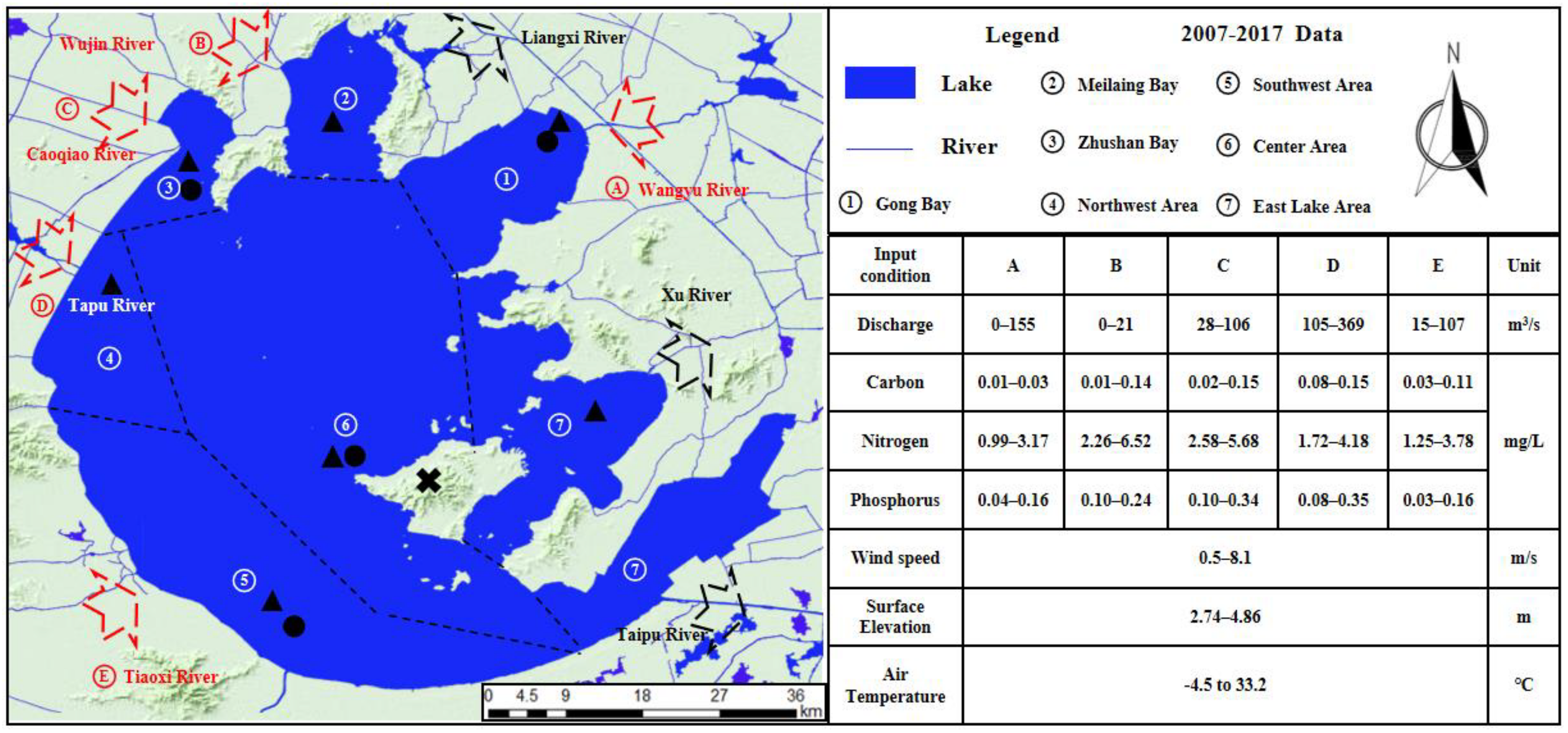
Tai Lake (119°08′~122°55′ E, 30°05′~32°08′ N) is the third-largest freshwater lake in China after Poyang Lake in Jiangxi and Dongting Lake in Hunan. Under the control of the surrounding artificial dams, the water depth ranges from 0 to 2 m. It is a typical shallow lake and is easily affected by the external environment [18]. To accurately determine the assessment area of Tai Lake, this study divided the lake into seven main areas: Gongwan Bay, Meiliang Bay, Zhushan Bay, the Northwest Lake area, the Southwest Lake area, the Center area, and the East Lake area, according to the comprehensive characteristics of the lake. The average measured water quality of the seven points was used as the model calibration target [19]. According to the relevant data collected in the past 10 years, such as water quantity, water quality, wind speed, water elevation, and temperature (http://lake.geodata.cn/data/dataresource.html) (accessed on 24 May 2020), combined with the later planning and actual situation, seven main external input conditions were selected, and their value ranges were determined (Figure 1).
2.2. Methodology
2.2.1. Eco-Lab Model
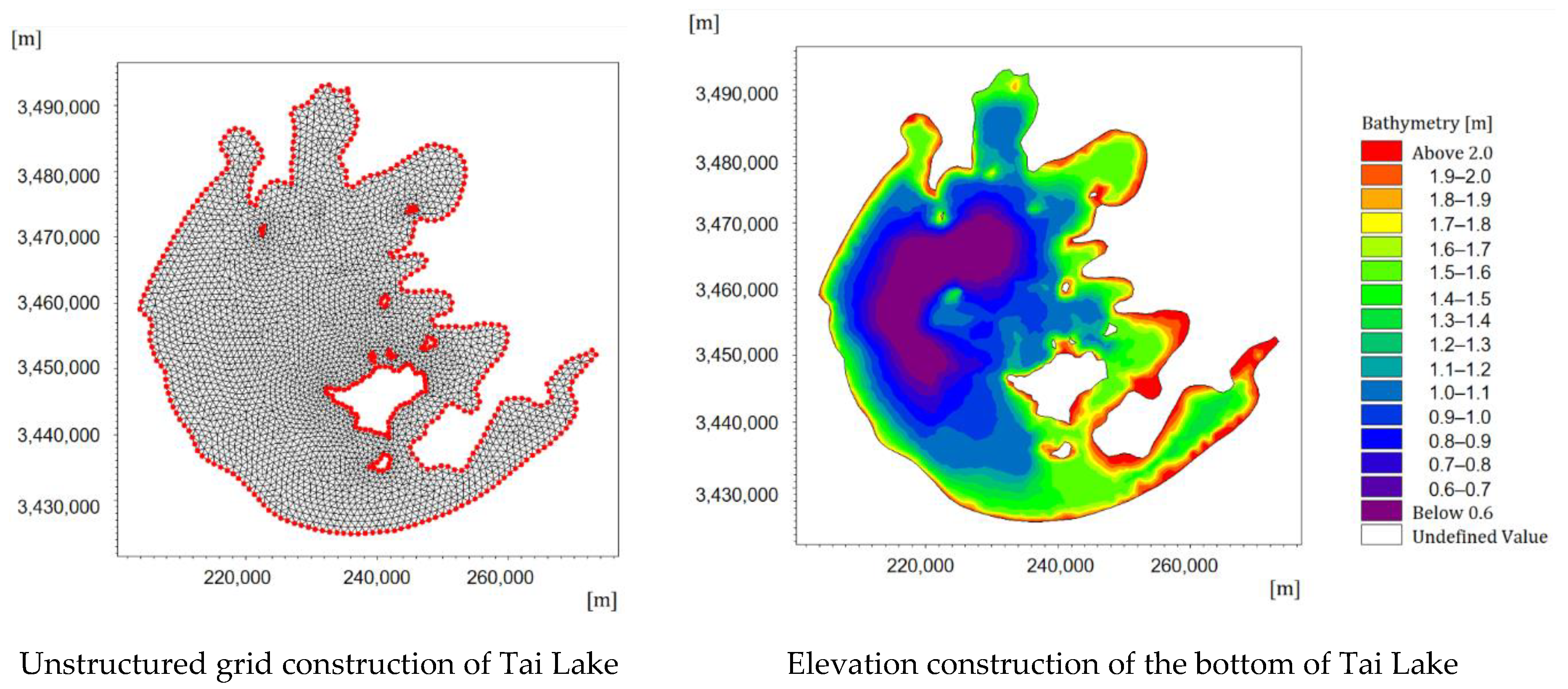
The Eco-lab model is based on a three-dimensional unsteady hydrodynamic model [20]. The model employed in this study featured a Cartesian coordinate grid of 5881 rectangular cells, each of which had a length of 300–500 m (Figure 2). To better simulate the lake bottom terrain, σ coordinates were used in the vertical direction, which was divided into three layers on average. According to the hydrostatic continuity and to avoid the pressure gradient error caused by the σ coordinate, the slope of the lake bottom should be less than 0.33. The model calculation time step was 3600 s, and the simulation time was 365 day.
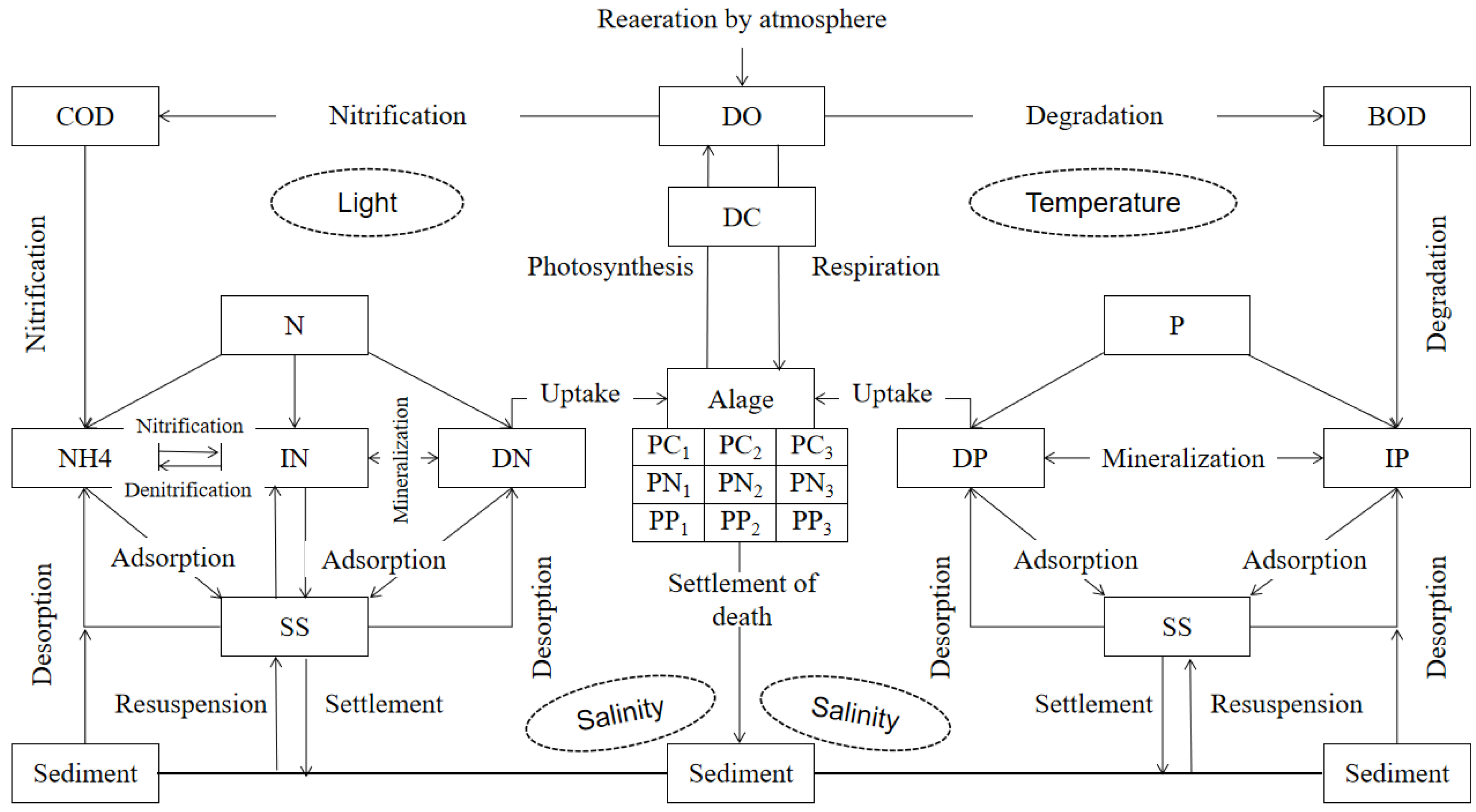
In order to simulate the material exchange in the water and algae growth more completely, the material exchange at the water–gas interface and the water–sediment interface were considered (Figure 3). The water–gas interface is mainly affected by the illumination, temperature, rainfall evaporation, and wind field [21]. The water–sediment interface is mainly determined by the nutrient release–absorption coefficient, reoxygenation coefficient, and salinity of the bottom mud. The most important water body is mainly composed of the nitrogen cycle, phosphorus cycle, and carbon cycle, combined with the correlation between dissolved oxygen and algae [22]. The three-dimensional hydrodynamic ecological model adopted in this study contained a total of 39 important parameters that needed calibration and verification (see the attachment for details), which involved the relevant important processes listed above and avoided the influence of uncertainty within the model.
2.2.2. LHS Uncertainty Analysis Method
Latin hypercube sampling [23] is an optimization method of uncertainty analysis based on the Monte Carlo method. In the calculation result statistics of the LHS method, N k-dimensional variable group values produce a total of n predicted values, and the n predicted values are arranged by size; the cumulative probability assigned to the smallest predicted value is 1/n, the cumulative probability assigned to the next smallest predicted value is 2/n, and so on, and the empirical distribution function of the predicted value is obtained. This empirical distribution function provides sample quantiles, that is, the mth predicted value is the sub-sample quantile of m/n × 100%. The 5% and 95% percentile values represent the uncertainty boundary caused by the parameter, 5% represents the lower boundary, and 95% represents the upper boundary. The specific process is as follows:
Step 1—Parameter grouping: group the input parameters or boundary conditions (m) into equal probability (n groups).
Step 2—Sampling combination: each parameter or boundary condition is randomly sampled in the value range of each different group n, which is recorded as x(1), x(2), …, xm, and an m × n matrix is formed after sampling a certain number of parameters according to the demand.
Step 3—Model calculation: bring each group of factors into the model for calculation until all factor groups are simulated. Because the model requires a long time for calculation, this study used 40 central procession unit calculations in parallel, which were performed 25 times in a row and run a total of 1000 times.
Step 4—Predicted value ranking: sort the n predicted values obtained by simulation according to size.
Step 5—Quantile determination: the cumulative probability assigned to the smallest predicted value is 1/n, the second smallest assigned is 2/n, and so on until all subsample quantiles are obtained, of which the m input result is m/n × 100%.
Step 6—Uncertain boundary selection: Choose 5% and 95% to represent the uncertainty boundary caused by the factor as the lower and upper boundaries, respectively.
In order to study and analyze the uncertainty of the input conditions, this paper, based on the basic scope of the region in the past 10 years (Figure 1), set the inflow and outflow, water quality, and wind speed to the original 50–150% and set the water level to the original. Some were plus or minus 0.6 m, and the temperature was set to the original plus or minus 5 °C (Table 1).
2.2.3. Morris Sensitivity Analysis Method
The Morris method [24] is a type of screening method, which is suitable for nonlinear models with a large number of factors, and the calculation speed is fast. At the same time, the improved Morris index can also be quantitatively analyzed. It is a design based on the one-at-a-time method, and through the spatial network sampling of all factors, a series of local partial derivatives are obtained:
where is the basic influence of the ith factor, f(x) represents the initial point of the trajectory, N represents the number of model factors, and is the size of the disturbance grid. The sensitivity index () and the interaction between the factors () can be calculated using Equations (2) and (3), respectively:
where is the influence result of the ith factor on the track j.
3. Results and Discussion
3.1. Calibration and Validation
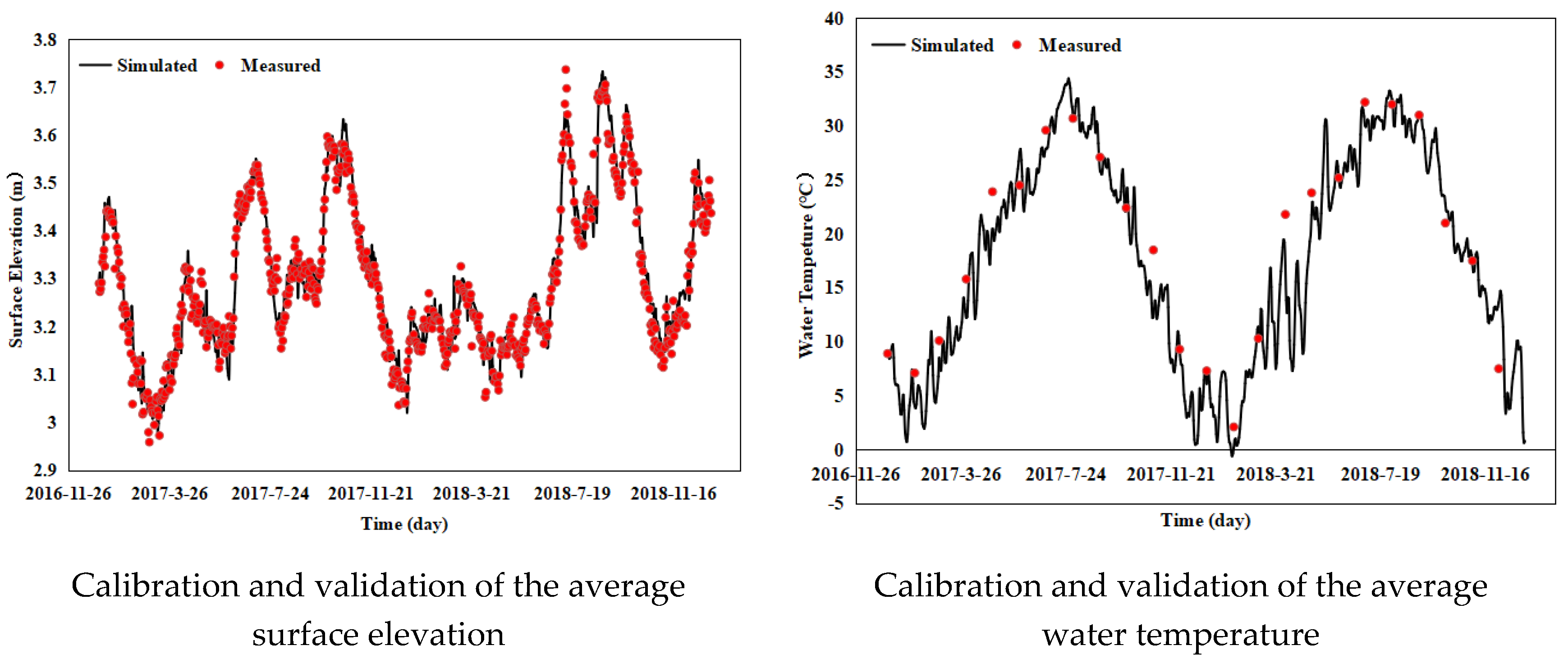
After calibration and verification of the surface elevation and water temperature of the lake during 2017–2018, the coefficient of turbulence, the height of the bottom friction, and the wind drag coefficient were estimated at 0.28, 0.02, and 0.003 m, respectively. The Dalton constant was 0.5, the transfer coefficient for heating was 0.015, and the transfer coefficient for cooling was 0.02. The error of the surface elevation and water temperature were both below 0.10 (Figure 4), indicating that the analysis can support further research.
According to the monthly monitoring data of Tai Lake in 2017 and 2018, the key parameters of the model were simulated (Appendix A). It was found that when the values of the parameters were as shown in the attachment, the calibration result in 2017 was better, and the verification result in 2018 was slightly worse than that of 2017, but the overall error was still within the model evaluation target (within 20%) [7]. At the same time, we found that the variation trend of Chl-a was similar to that of TP, indicating that TN met the basic requirements for the growth of Chl-a in Tai Lake, while the demand for the TP nutrient source was still limited by a certain threshold, which was consistent with the research results of many researchers [25,26,27]. The effects of nutrients and light on the growth of Chl-a were also different in different seasons. Chl-a was mostly influenced by light and temperature in the winter but mostly influenced by TP in the warmer seasons. The maximum influence of TP on Chl-a can reach about 35% [28]. The change trends of TN and DO were relatively similar. This was because both the nitrogen nitrification and denitrification reactions in the water–air cycle were related to the DO. It has been found that DO reduced the concentration of TN because of strengthened denitrification in 2018 [29,30]. The results showed that this model can simulate the trend and numerical value of the four water quality indexes well in the setting with relevant parameters and the simulation of the measured data (Figure 5). It can be preliminarily confirmed that the Eco-lab model has a good foundation in the water quality simulation of Tai Lake and can provide scientific support for further research in the future.
In order to further the comparison between the simulation results and the real value of the water level, this study adopted the average relative error (MRE), root mean square error (RMSE), analysis of correlation coefficient (R2), and the coefficient of Nash model (NSE) to evaluate the measured data (M) and the simulated data (S). The specific formulas are as follows [31]:
where N is the total number of simulations, i is the number of simulations, Si is the value of the ith simulation, Mi is the value measured in the ith simulation, the simulated average, and the measured average value.
The results show that the Eco-lab model has high credibility in the water quality simulation of Tai Lake with a comprehensive error within 20% (Table 2), which can better reflect the actual water quality in 2017 and 2018. These results are not only consistent with the trend of actual measurement results, but they are also consistent with the research conclusions of Wang et al. [32]. This proves once again that the Eco-lab water quality model can provide basic support for subsequent mechanism research.
3.2. Spatiotemporal Uncertainty Analysis of the Input Conditions
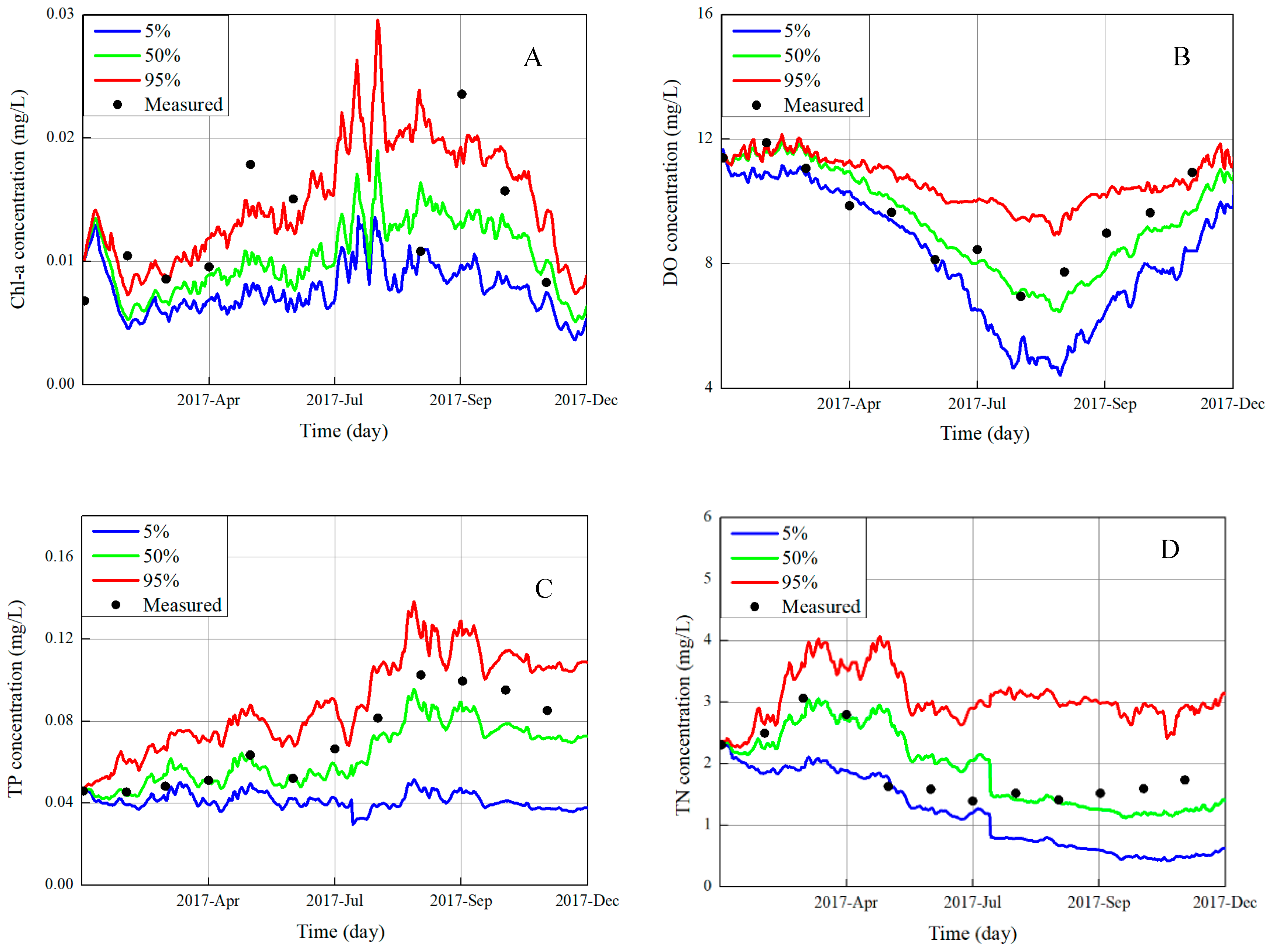
The input conditions have uncertainties related to four major indicators. Most of the measured values were within the calculation range, indicating that the model constructed in this study is scientific and reasonable (Figure 6) and can provide a scientific basis for further research. Some of the measured values of Chl-a and DO could not be included; this is because a dynamically balanced ecosystem has formed inside the lake. When the external input conditions change, the internal conditions respond accordingly [33]. This shows that the degree of influence by the external factors is lower than that by the internal parameters, which also gives Chl-a a more stable growth environment; this inference can also be verified by the minimum total phosphorus (TP) concentration. The dissolved oxygen (DO) concentration is mainly related to temperature and water elevation [34], and the uncertainty in summer and autumn is significantly greater than that in spring and winter, which is caused by the greater algae respiration in summer and autumn. The TN and TP concentrations are more affected by external factors than internal parameters [35] and thus represent a real problem. This phenomenon explains that land pollution control will play a more direct role in achieving the pollution control goal of Tai Lake, while controlling the Chl-a level will require a longer period to restore the lake’s health [36].
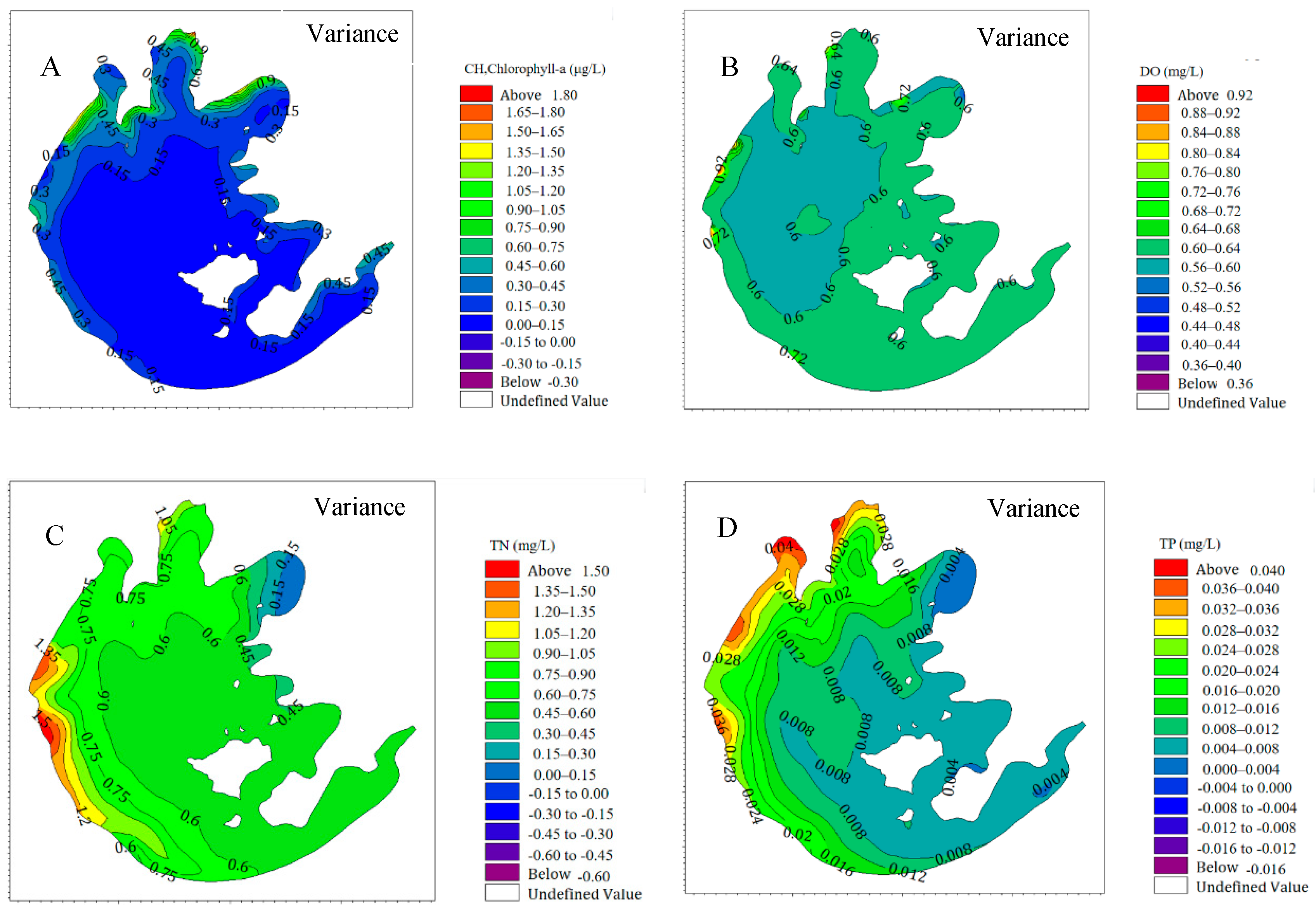
From the ANOVA results of 5881 grid cells in the lake (Figure 7), it was found that the spatial uncertainty of Chl-a mainly occurred in areas with heavy pollution or low water elevations [37]; the center area was still mainly affected by internal parameters, which further verifies the previous inference; and the uncertainty of DO occurred in the whole lake, mainly in areas with low water elevations, because DO is more stable in areas with higher water elevations [38] that are not easily affected by external factors. The main uncertainties of TN and TP occurred in the input area of the pollution source, especially the main entrance areas of the lake. This is because the internal parameters of the lake body require a longer time to respond to the instantaneous input of external pollutants [39]. According to the research results of the spatial uncertainty of Lake Tai, it was shown that the water quality (TN and TP) concentration of the main water body at the input of the lake is directly affected by land pollution sources, and the uncertainty phenomenon is very obvious. The uncertainty of Chl-a is smaller, that is, the control of Chl-a takes longer than that of a single source of pollution, such as TN and TP. Therefore, it was verified that land pollution control will have a direct impact on the lake’s water quality, while controlling the Chl-a level will take longer to achieve significant results [11].
3.3. Vertical Sensitivity Analysis of the Input Conditions
To conduct a more in-depth study on the vertical sensitivity of the water quality, the lake body was divided into a surface layer, middle layer, and bottom layer (Figure 8). Using the Morris method, the spatial sensitivity of external factors was further studied and analyzed. The results showed that the Chl-a and DO of the surface layer were affected by all external input conditions except nitrogen; among the conditions, wind speed, flow rate, and phosphorus were the main controlling factors of Chl-a [40], and the total sensitivity was 74%, indicating that Chl-a is easily affected by hydrodynamic conditions and has a certain synergy with phosphorus [41]. Temperature and water elevation were the main controlling factors of DO, with a sensitivity of 58%, and because of the organic matter degradation for oxygen consumption, DO is also affected by the organic matter content [42]. The changes in TN and TP were relatively clear. The flux (flow and concentration) into the lake was the main controlling factor, and the sensitivities were 93% (for flow) and 81% (for concentration), both exceeding 80%. The main controlling factors and sensitivity weights of DO, TN, and TP in the middle layer were similar to those of DO, TN, and TP in the surface layer, but Chl-a was significantly enhanced by the wind speed, and the sensitivity was about 42%. Wind speed is speculated to have the most significant effect on the hydrodynamic force of the middle layer, which in turn changes the growth conditions of algae [43]. Therefore, attention should be paid to avoid a large amount of water diversion during an algae outbreak. Although such a diversion can alleviate the local hydration crisis in the short term, it increases the risk of the water environment in the long run. The main controlling factors of all water quality indicators were more remarkable at the bottom; the DO concentration was almost inversely proportional to the temperature [44]. The bottom-layer DO changed by about 98% in response to temperature, indicating that the temperature of the Tai Lake water body is almost stable until it reaches the bottom layer, which is equivalent to the subsurface layer of deep-water lakes. Therefore, there is no thermocline in Tai Lake [45].
In general, the TP and TN in the three water layers, which could reach 78% and 83% on average, respectively, were greatly affected by external input flow and chemical concentrations, indicating that land pollution control will effectively reduce the average water quality of the lake. The development in the water quality of the lake verifies that a certain level of pollution control of the Tai Lake Basin has been achieved in recent years [46]. The DO concentration was mainly affected by temperature and water elevation, and the closer to the bottom, the more significant the effect of temperature on the DO. The main influencing factor of Chl-a was wind speed, and the average sensitivity was about 34%. The factors affecting the bottom layer were clearer, and the fluctuation of the related water quality parameters was also smaller. This verifies that shallow lakes are easily disturbed by external conditions, while deep lakes are more stable [47].
To further explain the mechanism of the effect of external input conditions on algae growth, this study combined the basic findings of multiple researchers (Table 3) with the calculation results of this study. The wind speed and flow into Tai Lake were found to play a key role in algae growth [28]. This is because hydrodynamic conditions mainly cause changes in light intensity, cell length, nutrient transport, and predation behavior, and they all directly affect algae growth [48,49]. First, the enhancement in the hydrodynamic force leads to increased resuspension of sediments at the lake bottom. The lake interior is equivalent to a nutrient reservoir; it can provide a continuous source of nutrients for algae growth [50]. In one study, after strong winds (12 m/s) and weak winds lasted for many days, the Meiliang Bay area of Tai Lake was tested. It was found that when the bottom sediment was about 20 cm, compared with the period of strong wind and waves, the suspended matter concentration in the lake water increased 10-fold, and the total phosphorus concentration increased nearly 3.6-fold [51]. Second, changes in hydrodynamic conditions can also cause changes in the structure of algae populations, mainly manifested in the dominant population conversion caused by the intensification of water mixing [52,53]; the self-depletion of a single dominant algae population is inhibited, and the survival time of algae is promoted. Finally, large disturbances in the water body also reduce the water body transparency and inhibit the growth of submerged vegetation [54]. This further creates superior conditions for the growth and spread of algae, which are some of the causes of the algae concentration on the surface layer.
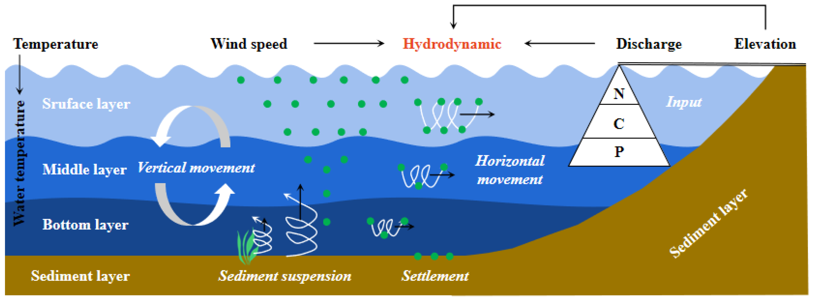
By studying the relationship between external factors and algae in the lake (Figure 9), we found that the lake water quality can be quickly improved through land pollution control, but the treatment of algae outbreaks in large shallow lakes cannot be realized in a short period of time [22]. This is because the current internal nutrients of Tai Lake can still be rebalanced by sediments to achieve the dynamic balance to meet the algae growth needs. Wind speed, flow, and water elevation are the key factors affecting the lake flow field, of which wind speed is the most critical factor affecting hydrodynamics [15,58]. It is also a factor currently beyond human control, which also reflects the cause of the basically controllable pollution of Tai Lake. However, the phenomenon of algal storms is still frequent. Therefore, we hope that this study provides solutions for the continuous control of land pollution sources and the strict control of the scale of water diversion to reduce the flux of external pollution input. Moreover, this study can provide guidance to strengthen the restoration of lake water ecosystems to mitigate the impact of wind and reduce the sediment resuspension ratio. Finally, gradually reducing the endogenous nutrient level can inhibit algae growth [59,60].
4. Conclusions
Based on the measured basic data, the LHS and Morris analysis methods were used to analyze the uncertainty and sensitivity of input conditions for Tai Lake. It is mainly studied and discussed from three aspects of climatic conditions, water quality conditions, and hydrodynamic conditions, and the specific conclusions are as follows:
(1) Input conditions were found to have significant impacts on the four major indicators of Tai Lake. Among them, Chl-a and DO had major impacts in the lake’s center area, and the impacts on TP and TN were mainly concentrated in the inflow area. The impacts of TN and TP were greater than those of Chl-a and DO, indicating that catchment pollution control can directly and quickly affect the water quality. However, altering the Chl-a level will require a longer time to achieve a significant impact.
(2) Different water layers exhibited different response mechanisms to the lake indicators. The surface and middle layers were similarly affected by input conditions. The bottom layer was most significantly and stably affected by input conditions. Overall, the TN and TP in the three water layers were closely related to the flux into the lake, and their average sensitivities were 83% and 78%, respectively. The DO concentration was mainly related to temperature and water elevation; the average sensitivity of the DO to temperature was 69%, and in the bottom layer, the DO changed by as much as ~98% in response to temperature. The Chl-a level was affected by all input factors except nitrogen and was most affected by wind speed, with an average sensitivity of about 34%.
(3) This study can provide guidance for the control of land pollution sources and the strict control of the water diversion scale to reduce the external pollution input fluxes. Moreover, it can help strengthen the restoration of lake water ecosystems to mitigate the impact of wind and reduce the sediment resuspension ratio. Finally, gradually reducing the endogenous nutrient level can inhibit algae growth in the future.
Author Contributions
Conceptualization, M.P. and R.X.; methodology, M.P.; software, Z.H.; validation, Z.H., J.W. and Y.W.; formal analysis, M.P.; investigation, R.X.; resources, R.X.; data curation, Z.H.; writing—original draft preparation, M.P.; writing—review and editing, R.X.; visualization, Z.H.; supervision, R.X.; funding acquisition, M.P. All authors have read and agreed to the published version of the manuscript.
Funding
This research was funded by Chinese National Science Foundation (Grant No. 52000100), Chinese National Science Foundation (Grant No. 51879070), Central Universities (No. 2019B44214) and PAPD, Major Science and Technology Program for Water Pollution Control and Treatment (Grant No. 2018ZX07208003). and “The APC was funded by Chinese National Science Foundation (Grant No. 51879070)”.
Institutional Review Board Statement
Not applicable.
Informed Consent Statement
Not applicable.
Data Availability Statement
Not applicable.
Conflicts of Interest
The authors declare no conflict of interest.
Appendix A

Table A1.
Calibration of key parameters of the Eco-lab model.
| Parameters | Calibration | Unit | Parameters | Calibration | Unit |
|---|---|---|---|---|---|
| mymg | 2.1 | (d) | prel | 0.003 | g P/m2/day |
| sep | 0.15 | (d) | ters | 1.02 | dimensionless |
| seve | 0.1 | meter/day | pnmi | 0.08 | g N/g C |
| kdma | 0.05 | (d) | pnma | 0.13 | g N/g C |
| kra | 3 | (d) | ppmi | 0.006 | g P/g C |
| kmdm | 0.02 | (d) | ppma | 0.08 | g P/g C |
| pla | 20 | m2/g Chl-a | kc | 0.005 | g P/g C |
| bla | 0.456 | m2 | kni | 0.15 | g N/g C/day |
| kmsc | 1 | dimensionless | kpi | 0.008 | g P/g C/day |
| kmsn | 0.3 | dimensionless | kpn | 0.2 | g N/m3 |
| kmsp | 0.8 | dimensionless | kpp | 0.02 | g P/m3 |
| mdo | 5.5 | mg/L | vm | 0.1 | dimensionless |
| mdos | 3.5 | mg/L | fac | 1.3 | dimensionless |
| ndo | 1.03 | dimensionless | alfaeu | 25 | E/m2/d |
| tere | 1.04 | dimensionless | teti | 1.05 | dimensionless |
| kmdn | 1 | dimensionless | epsi | 0.005 | dimensionless |
| kmdp | 1 | dimensionless | vo | 3.5 | g DO/g C |
| tetn | 1.02 | dimensionless | lcg | 0.16 | (d) |
| tetp | 1.02 | dimensionless | optg | 28 | (d) |
| nrel | 0.02 | g N/m2/day |
References
- Wang, H.; Zhang, Z.; Liang, D.; Pang, Y.; Hu, K.; Wang, J. Separation of wind’s influence on harmful cyanobacterial blooms. Water Res. 2016, 98, 280–292. [Google Scholar] [CrossRef]
- Zhang, P.; Liang, R.-F.; Zhao, P.-X.; Liu, Q.-Y.; Li, Y.; Wang, K.-L.; Li, K.-F.; Liu, Y.; Wang, P. The Hydraulic Driving Mechanisms of Cyanobacteria Accumulation and the Effects of Flow Pattern on Ecological Restoration in Lake Dianchi Caohai. Int. J. Environ. Res. Public Health 2019, 16, 361. [Google Scholar] [CrossRef] [Green Version]
- D’Andrea, M.F.; Letourneau, G.; Rousseau, A.N.; Brodeur, J.C. Sensitivity analysis of the Pesticide in Water Calculator model for applications in the Pampa region of Argentina. Sci. Total Environ. 2020, 698, 134232. [Google Scholar] [CrossRef]
- Hübler, C. Global sensitivity analysis for medium-dimensional structural engineering problems using stochastic collocation. Reliab. Eng. Syst. Saf. 2020, 195, 106749. [Google Scholar] [CrossRef]
- Douglas-Smith, D.; Iwanaga, T.; Croke, B.F.W.; Jakeman, A.J. Certain trends in uncertainty and sensitivity analysis: An overview of software tools and techniques. Environ. Model. Softw. 2020, 124, 104588. [Google Scholar] [CrossRef]
- Naves, J.; Rieckermann, J.; Cea, L.; Puertas, J.; Anta, J. Global and local sensitivity analysis to improve the understanding of physically-based urban wash-off models from high-resolution laboratory experiments. Sci. Total Environ. 2020, 709, 136152. [Google Scholar] [CrossRef] [PubMed]
- Page, T.; Smith, P.; Beven, K.; Jones, I.; Elliott, J.; Maberly, S.; Mackay, E.; De Ville, M.; Feuchtmayr, H. Constraining uncertainty and process-representation in an algal community lake model using high frequency in-lake observations. Ecol. Model. 2017, 357, 1–13. [Google Scholar] [CrossRef] [Green Version]
- Silva, A.S.; Ghisi, E. Estimating the sensitivity of design variables in the thermal and energy performance of buildings through a systematic procedure. J. Clean. Prod. 2020, 244, 118753. [Google Scholar] [CrossRef]
- Pearson, J.; Dunham, J.; Bellmore, J.R.; Lyons, D. Modeling control of Common Carp (Cyprinus carpio) in a shallow lake–wetland system. Wetl. Ecol. Manag. 2019, 27, 663–682. [Google Scholar] [CrossRef]
- Xiong, Q.; Gou, J.; Mao, H.; Shan, J. Optimization of sensitivity analysis in best estimate plus uncertainty and the application to large break LOCA of a three-loop pressurized water reactor. Prog. Nucl. Energy 2020, 126, 103396. [Google Scholar] [CrossRef]
- Jiang, L.; Li, Y.; Zhao, X.; Tillotson, M.R.; Wang, W.; Zhang, S.; Sarpong, L.; Asmaa, Q.; Pan, B. Parameter uncertainty and sensitivity analysis of water quality model in Lake Taihu, China. Ecol. Model. 2018, 375, 1–12. [Google Scholar] [CrossRef]
- Qian, G.; Mahdi, A. Sensitivity analysis methods in the biomedical sciences. Math. Biosci. 2020, 323, 108306. [Google Scholar] [CrossRef] [PubMed]
- Peng, X.; Adamowski, J.; Inam, A.; Alizadeh, M.R.; Albano, R. Development of a behaviour-pattern based global sensitivity analysis procedure for coupled socioeconomic and environmental models. J. Hydrol. 2020, 585, 124745. [Google Scholar] [CrossRef]
- Jaxa-Rozen, M.; Kwakkel, J. Tree-based ensemble methods for sensitivity analysis of environmental models: A performance comparison with Sobol and Morris techniques. Environ. Model. Softw. 2018, 107, 245–266. [Google Scholar] [CrossRef]
- Li, Y.; Tang, C.; Zhu, J.; Pan, B.; Anim, D.O.; Ji, Y.; Yu, Z.; Acharya, K. Parametric uncertainty and sensitivity analysis of hydrodynamic processes for a large shallow freshwater lake. Hydrol. Sci. J. 2015, 60, 1078–1095. [Google Scholar] [CrossRef]
- Bellin, N.; Groppi, M.; Rossi, V. A model of egg bank dynamics in ephemeral ponds. Ecol. Model. 2020, 430, 109126. [Google Scholar] [CrossRef]
- Koo, H.; Chen, M.; Jakeman, A.J.; Zhang, F. A global sensitivity analysis approach for identifying critical sources of uncertainty in non-identifiable, spatially distributed environmental models: A holistic analysis applied to SWAT for input datasets and model parameters. Environ. Model. Softw. 2020, 127, 104676. [Google Scholar] [CrossRef]
- Tao, Y.; Dan, D.; Xuejiao, H.; Changda, H.; Guo, F.; Fengchang, W. Characterization of phosphorus accumulation and release using diffusive gradients in thin films (DGT)—Linking the watershed to Taihu Lake, China. Sci. Total Environ. 2019, 673, 347–356. [Google Scholar] [CrossRef]
- Li, Y.; Tang, C.; Wang, J.; Acharya, K.; Du, W.; Gao, X.; Luo, L.; Li, H.; Dai, S.; Mercy, J.; et al. Effect of wave-current interactions on sediment resuspension in large shallow Lake Taihu, China. Environ. Sci. Pollut. Res. Int. 2017, 24, 4029–4039. [Google Scholar] [CrossRef]
- Waldman, S.; Bastón, S.; Nemalidinne, R.; Chatzirodou, A.; Venugopal, V.; Side, J. Implementation of tidal turbines in MIKE 3 and Delft3D models of Pentland Firth & Orkney Waters. Ocean Coast. Manag. 2017, 147, 21–36. [Google Scholar]
- Han, Y.; Fang, H.; Huang, L.; Li, S.; He, G. Simulating the distribution of Corbicula fluminea in Lake Taihu by benthic invertebrate biomass dynamic model (BIBDM). Ecol. Model. 2019, 409, 108730. [Google Scholar] [CrossRef]
- Janssen, A.B.G.; de Jager, V.C.L.; Janse, J.H.; Kong, X.; Liu, S.; Ye, Q.; Mooij, W.M. Spatial identification of critical nutrient loads of large shallow lakes: Implications for Lake Taihu (China). Water Res. 2017, 119, 276–287. [Google Scholar] [CrossRef] [PubMed]
- Sheikholeslami, R.; Razavi, S. Progressive Latin Hypercube Sampling: An efficient approach for robust sampling-based analysis of environmental models. Environ. Model. Softw. 2017, 93, 109–126. [Google Scholar] [CrossRef]
- Ren, J.; Zhang, W.; Yang, J. Morris Sensitivity Analysis for Hydrothermal Coupling Parameters of Embankment Dam: A Case Study. Math. Probl. Eng. 2019, 2019, 1–11. [Google Scholar] [CrossRef] [Green Version]
- Zou, R.; Wu, Z.; Zhao, L.; Elser, J.J.; Yu, Y.; Chen, Y.; Liu, Y. Seasonal algal blooms support sediment release of phosphorus via positive feedback in a eutrophic lake: Insights from a nutrient flux tracking modeling. Ecol. Model. 2020, 416, 108881. [Google Scholar] [CrossRef]
- Zhang, S.; Yi, Q.; Buyang, S.; Cui, H.; Zhang, S. Enrichment of bioavailable phosphorus in fine particles when sediment resuspension hinders the ecological restoration of shallow eutrophic lakes. Sci. Total Environ. 2020, 710, 135672. [Google Scholar] [CrossRef]
- Wu, T.; Qin, B.; Brookes, J.D.; Yan, W.; Ji, X.; Feng, J. Spatial distribution of sediment nitrogen and phosphorus in Lake Taihu from a hydrodynamics-induced transport perspective. Sci. Total Environ. 2019, 650 Pt 1, 1554–1565. [Google Scholar] [CrossRef]
- Deng, J.; Zhang, W.; Qin, B.; Zhang, Y.; Paerl, H.W.; Salmaso, N. Effects of climatically-modulated changes in solar radiation and wind speed on spring phytoplankton community dynamics in Lake Taihu, China. PLoS ONE 2018, 13, e0205260. [Google Scholar] [CrossRef]
- Nizzoli, D.; Welsh, D.T.; Viaroli, P. Denitrification and benthic metabolism in lowland pit lakes: The role of trophic conditions. Sci. Total Environ. 2020, 703, 134804. [Google Scholar] [CrossRef] [PubMed]
- Schafer, C.; Ho, J.; Lotz, B.; Armbruster, J.; Putz, A.; Zou, H.; Li, C.; Ye, C.; Zheng, B.; Hugler, M.; et al. Evaluation and application of molecular denitrification monitoring methods in the northern Lake Tai, China. Sci. Total Environ. 2019, 663, 686–695. [Google Scholar] [CrossRef]
- Xu, R.; Pang, Y.; Hu, Z.; Kaisam, J.P. Dual-Source Optimization of the “Diverting Water from the Yangtze River to Tai Lake (DWYRTL)” Project Based on the Euler Method. Complexity 2020, 2020, 1–12. [Google Scholar] [CrossRef]
- Wang, J.; Zhao, Q.; Pang, Y.; Li, Y.; Yu, Z.; Wang, Y. Dynamic simulation of sediment resuspension and its effect on water quality in Lake Taihu, China. Water Sci. Technol. Water Supply 2017, 17, 1335–1346. [Google Scholar] [CrossRef]
- Wang, M.; Strokal, M.; Burek, P.; Kroeze, C.; Ma, L.; Janssen, A.B.G. Excess nutrient loads to Lake Taihu: Opportunities for nutrient reduction. Sci. Total Environ. 2019, 664, 865–873. [Google Scholar] [CrossRef]
- Terry, J.A.; Sadeghian, A.; Lindenschmidt, K.-E. Modelling Dissolved Oxygen/Sediment Oxygen Demand under Ice in a Shallow Eutrophic Prairie Reservoir. Water 2017, 9, 131. [Google Scholar] [CrossRef] [Green Version]
- Wang, L.; Wang, Y.; Cheng, H.; Cheng, J. Estimation of the Nutrient and Chlorophyll a Reference Conditions in Taihu Lake Based on A New Method with Extreme(-)Markov Theory. Int. J. Environ. Res. Public Health 2018, 15, 2372. [Google Scholar] [CrossRef] [Green Version]
- Yang, Z.; Zhang, M.; Shi, X.; Kong, F.; Ma, R.; Yu, Y. Nutrient reduction magnifies the impact of extreme weather on cyanobacterial bloom formation in large shallow Lake Taihu (China). Water Res. 2016, 103, 302–310. [Google Scholar] [CrossRef]
- Li, C.; Feng, W.; Chen, H.; Li, X.; Song, F.; Guo, W.; Giesy, J.P.; Sun, F. Temporal variation in zooplankton and phytoplankton community species composition and the affecting factors in Lake Taihu-a large freshwater lake in China. Environ. Pollut. 2019, 245, 1050–1057. [Google Scholar] [CrossRef]
- García-Nieto, P.J.; García-Gonzalo, E.; Sánchez Lasheras, F.; Alonso Fernández, J.R.; Díaz Muñiz, C. A hybrid DE optimized wavelet kernel SVR-based technique for algal atypical proliferation forecast in La Barca reservoir: A case study. J. Comput. Appl. Math. 2020, 366, 112417. [Google Scholar] [CrossRef]
- Sun, X.; Choi, Y.Y.; Choi, J.-I. Global sensitivity analysis for multivariate outputs using polynomial chaos-based surrogate models. Appl. Math. Model. 2020, 82, 867–887. [Google Scholar] [CrossRef]
- Dai, J.; Wu, S.; Wu, X.; Xue, W.; Yang, Q.; Zhu, S.; Wang, F.; Chen, D. Effects of Water Diversion from Yangtze River to Lake Taihu on the Phytoplankton Habitat of the Wangyu River Channel. Water 2018, 10, 759. [Google Scholar] [CrossRef] [Green Version]
- Yan, C.; Che, F.; Zeng, L.; Wang, Z.; Du, M.; Wei, Q.; Wang, Z.; Wang, D.; Zhen, Z. Spatial and seasonal changes of arsenic species in Lake Taihu in relation to eutrophication. Sci. Total Environ. 2016, 563–564, 496–505. [Google Scholar] [CrossRef]
- García Nieto, P.J.; García-Gonzalo, E.; Alonso Fernández, J.R.; Díaz Muñiz, C. Water eutrophication assessment relied on various machine learning techniques: A case study in the Englishmen Lake (Northern Spain). Ecol. Model. 2019, 404, 91–102. [Google Scholar] [CrossRef]
- Deng, J.; Paerl, H.W.; Qin, B.; Zhang, Y.; Zhu, G.; Jeppesen, E.; Cai, Y.; Xu, H. Climatically-modulated decline in wind speed may strongly affect eutrophication in shallow lakes. Sci. Total Environ. 2018, 645, 1361–1370. [Google Scholar] [CrossRef]
- Ellina, G.; Papaschinopoulos, G.; Papadopoulos, B. The use of fuzzy estimators for the construction of a prediction model concerning an environmental ecosystem. Sustainability 2019, 11, 5039. [Google Scholar] [CrossRef] [Green Version]
- Vandenberg, J.; Litke, S. Beneficial Use of Springer Pit Lake at Mount Polley Mine. Mine Water Environ. 2018, 37, 663–672. [Google Scholar] [CrossRef]
- Li, Y.; Zhou, S.; Jia, Z.; Ge, L.; Mei, L.; Sui, X.; Wang, X.; Li, B.; Wang, J.; Wu, S. Influence of Industrialization and Environmental Protection on Environmental Pollution: A Case Study of Taihu Lake, China. Int. J. Environ. Res. Public Health 2018, 15, 2628. [Google Scholar] [CrossRef] [PubMed] [Green Version]
- Feng, T.; Wang, C.; Wang, P.; Qian, J.; Wang, X. How physiological and physical processes contribute to the phenology of cyanobacterial blooms in large shallow lakes: A new Euler-Lagrangian coupled model. Water Res. 2018, 140, 34–43. [Google Scholar] [CrossRef]
- Chao, J.Y.; Zhang, Y.M.; Kong, M.; Zhuang, W.; Wang, L.M.; Shao, K.Q.; Gao, G. Long-term moderate wind induced sediment resuspension meeting phosphorus demand of phytoplankton in the large shallow eutrophic Lake Taihu. PLoS ONE 2017, 12, e0173477. [Google Scholar] [CrossRef]
- Xu, D.; Wang, Y.; Liu, D.; Wu, D.; Zou, C.; Chen, Y.; Cai, Y.; Leng, X.; An, S. Spatial heterogeneity of food web structure in a large shallow eutrophic lake (Lake Taihu, China): Implications for eutrophication process and management. J. Freshw. Ecol. 2019, 34, 231–247. [Google Scholar] [CrossRef] [Green Version]
- Jalil, A.; Li, Y.; Du, W.; Wang, J.; Gao, X.; Wang, W.; Acharya, K. Wind-induced flow velocity effects on nutrient concentrations at Eastern Bay of Lake Taihu, China. Environ. Sci. Pollut. Res. Int. 2017, 24, 17900–17911. [Google Scholar] [CrossRef] [PubMed]
- Qin, B.; Xu, P.; Wu, Q.; Luo, L.; Zhang, Y. Environmental issues of Lake Taihu, China. Hydrobiologia 2007, 581, 3–14. [Google Scholar] [CrossRef]
- Guo, Y.; Yu, G.; Qin, B. Historical trophic evolution resulting from changes in climate and ecosystem in Lake Taihu and seven other lakes, China. J. Freshw. Ecol. 2015, 30, 25–40. [Google Scholar] [CrossRef]
- Gong, Y.; Tang, X.; Shao, K.; Hu, Y.; Gao, G. Dynamics of bacterial abundance and the related environmental factors in large shallow eutrophic Lake Taihu. J. Freshw. Ecol. 2017, 32, 133–145. [Google Scholar] [CrossRef] [Green Version]
- Gao, H.; Shi, Q.; Qian, X. A multi-species modelling approach to select appropriate submerged macrophyte species for ecological restoration in Gonghu Bay, Lake Taihu, China. Ecol. Model. 2017, 360, 179–188. [Google Scholar] [CrossRef]
- Jalil, A.; Li, Y.; Du, W.; Wang, W.; Wang, J.; Gao, X.; Khan, H.O.S.; Pan, B.; Acharya, K. The role of wind field induced flow velocities in destratification and hypoxia reduction at Meiling Bay of large shallow Lake Taihu, China. Environ. Pollut. 2018, 232, 591–602. [Google Scholar] [CrossRef]
- Tang, C.; Li, Y.; Acharya, K. Modeling the effects of external nutrient reductions on algal blooms in hyper-eutrophic Lake Taihu, China. Ecol. Eng. 2016, 94, 164–173. [Google Scholar] [CrossRef] [Green Version]
- Xu, H.; Paerl, H.W.; Qin, B.; Zhu, G.; Gaoa, G. Nitrogen and phosphorus inputs control phytoplankton growth in eutrophic LakeTaihu, China. Limnol. Oceanogr. 2010, 55, 420–432. [Google Scholar] [CrossRef] [Green Version]
- Liu, S.; Ye, Q.; Wu, S.; Stive, M.J.F. Horizontal circulation patterns in a large shallow lake: Taihu Lake, China. Water 2018, 10, 792. [Google Scholar] [CrossRef] [Green Version]
- Ke, Z.; Xie, P.; Guo, L. Ecological restoration and factors regulating phytoplankton community in a hypertrophic shallow lake, Lake Taihu, China. Acta Ecol. Sin. 2019, 39, 81–88. [Google Scholar] [CrossRef]
- Nazari-Sharabian, M.; Taheriyoun, M.; Ahmad, S.; Karakouzian, M.; Ahmadi, A. Water Quality Modeling of Mahabad Dam Watershed–Reservoir System under Climate Change Conditions, Using SWAT and System Dynamics. Water 2019, 11, 394. [Google Scholar] [CrossRef] [Green Version]
Figure 1.
The study area and the measured external factor value ranges in the last 10 years (the black triangle represents the water quality monitoring site of the main lake area, the black circle represents the location of the lake water level monitoring point, and the black cross represents the location of the lake meteorological monitoring point).

Figure 2.
Grid information and underwater bathymetry.

Figure 3.
Frame diagram of the Eco-lab model mechanism.

Figure 4.
Surface elevation and water temperature calibration and validation of Tai Lake from 2017 to 2018.
Figure 4.
Surface elevation and water temperature calibration and validation of Tai Lake from 2017 to 2018.

Figure 5.
Monthly error evaluation charts of the four major indicators (TP, TN, Chl-a, and DO) in the seven districts of Tai Lake from 2017 to 2018.
Figure 5.
Monthly error evaluation charts of the four major indicators (TP, TN, Chl-a, and DO) in the seven districts of Tai Lake from 2017 to 2018.

Figure 6.
Uncertainty analysis related to four water quality indicators during different time periods in Tai Lake: (A) Chl-a concentration; (B) DO, dissolved oxygen concentration; (C) TP, total phosphorus concentration; and (D) TN, total nitrogen concentration.
Figure 6.
Uncertainty analysis related to four water quality indicators during different time periods in Tai Lake: (A) Chl-a concentration; (B) DO, dissolved oxygen concentration; (C) TP, total phosphorus concentration; and (D) TN, total nitrogen concentration.

Figure 7.
Uncertainty analysis related to four water quality indicators in Tai Lake. (A) Chl-a concentration; (B) DO, dissolved oxygen concentration; (C) TN, total nitrogen concentration; (D) TP, total phosphorus concentration.
Figure 7.
Uncertainty analysis related to four water quality indicators in Tai Lake. (A) Chl-a concentration; (B) DO, dissolved oxygen concentration; (C) TN, total nitrogen concentration; (D) TP, total phosphorus concentration.

Figure 8.
Sensitivity analysis results of four water quality indicators in three different layers: (A) surface layer, (B) middle layer, (C) bottom layer. (D) Average sensitivity degree.
Figure 8.
Sensitivity analysis results of four water quality indicators in three different layers: (A) surface layer, (B) middle layer, (C) bottom layer. (D) Average sensitivity degree.

Figure 9.
Schematic diagram of the relationship between external input conditions and algae growth. The black bold terms represent the main external input conditions, the red bold terms represent the state of the lake body being directly changed, the white bold terms represent three water layers and a bottom mud layer, and the white italicized bold terms represent the response process within the system.

Table 1.
Determining the value range of different input conditions.
| Input Condition | Lower | Upper | Unit |
|---|---|---|---|
| Discharge | 50 | 150 | % |
| C | |||
| N | |||
| P | |||
| Wind speed | |||
| Surface elevation | −0.6 | 0.6 | m |
| Air temperature | −5 | 5 | °C |
Table 2.
Model calculation results of the four indexes of the seven lake regions.
| Indicators | Time | RMSE | MRE | R2 | NSE |
|---|---|---|---|---|---|
| TP | Calibration | 0.010 | 0.008 | 0.939 | 0.841 |
| Validation | 0.015 | 0.012 | 0.842 | 0.779 | |
| TN | Calibration | 0.207 | 0.170 | 0.938 | 0.990 |
| Validation | 0.309 | 0.244 | 0.925 | 0.959 | |
| Chl-a | Calibration | 0.006 | 0.005 | 0.847 | 0.992 |
| Validation | 0.008 | 0.006 | 0.829 | 0.988 | |
| DO | Calibration | 0.929 | 0.777 | 0.889 | 0.991 |
| Validation | 0.947 | 0.805 | 0.798 | 0.990 |
Table 3.
Research results on the relationship between external conditions and water quality in Tai Lake.
Table 3.
Research results on the relationship between external conditions and water quality in Tai Lake.
| External Factor | Method | Indicator | Conclusions | Reference |
|---|---|---|---|---|
| Wind, temperature | Experiment | Algal blooms, DO | Wind field plays a key role in algae growth. | [55] |
| Wind | Experiment | TN, TP | Wind field plays an important role in sediment resuspension. | [32] |
| Discharge, nitrogen, phosphorus | Model | Algal blooms | Lake ecological management still needs a long-term process. | [56] |
| Nitrogen, phosphorus | Experiment | Chl-a | Nutrients promote algae growth, but they are not the decisive factor in Tai Lake. | [57] |
| Surface elevation, nitrogen, phosphorus | Experiment | Chl-a | The vertical release of nitrogen and phosphorus in the sediment leads to the continued existence of algae. | [27] |
| Discharge, carbon, nitrogen, phosphorus, wind speed, surface elevation, temperature | Model | Chl-a, DO, TN, TP | The improvement in the hydrodynamic force promotes algae growth. The control of pollution input can effectively reduce the pollution concentration of the lake, but it cannot immediately solve the risk of an algae outbreak. | This study |
Publisher’s Note: MDPI stays neutral with regard to jurisdictional claims in published maps and institutional affiliations. |
© 2021 by the authors. Licensee MDPI, Basel, Switzerland. This article is an open access article distributed under the terms and conditions of the Creative Commons Attribution (CC BY) license (https://creativecommons.org/licenses/by/4.0/).
Share and Cite
MDPI and ACS Style
Pang, M.; Xu, R.; Hu, Z.; Wang, J.; Wang, Y. Uncertainty and Sensitivity Analysis of Input Conditions in a Large Shallow Lake Based on the Latin Hypercube Sampling and Morris Methods. Water 2021, 13, 1861. https://doi.org/10.3390/w13131861
AMA Style
Pang M, Xu R, Hu Z, Wang J, Wang Y. Uncertainty and Sensitivity Analysis of Input Conditions in a Large Shallow Lake Based on the Latin Hypercube Sampling and Morris Methods. Water. 2021; 13(13):1861. https://doi.org/10.3390/w13131861
Chicago/Turabian StylePang, Min, Ruichen Xu, Zhibing Hu, Jianjian Wang, and Ying Wang. 2021. "Uncertainty and Sensitivity Analysis of Input Conditions in a Large Shallow Lake Based on the Latin Hypercube Sampling and Morris Methods" Water 13, no. 13: 1861. https://doi.org/10.3390/w13131861
Note that from the first issue of 2016, this journal uses article numbers instead of page numbers. See further details here.