
Living Benthic Foraminifera from the Surface and Subsurface Sediment Layers Applied to the Environmental Characterization of the Brazilian Continental Slope (SW Atlantic)


Abstract
:1. Introduction
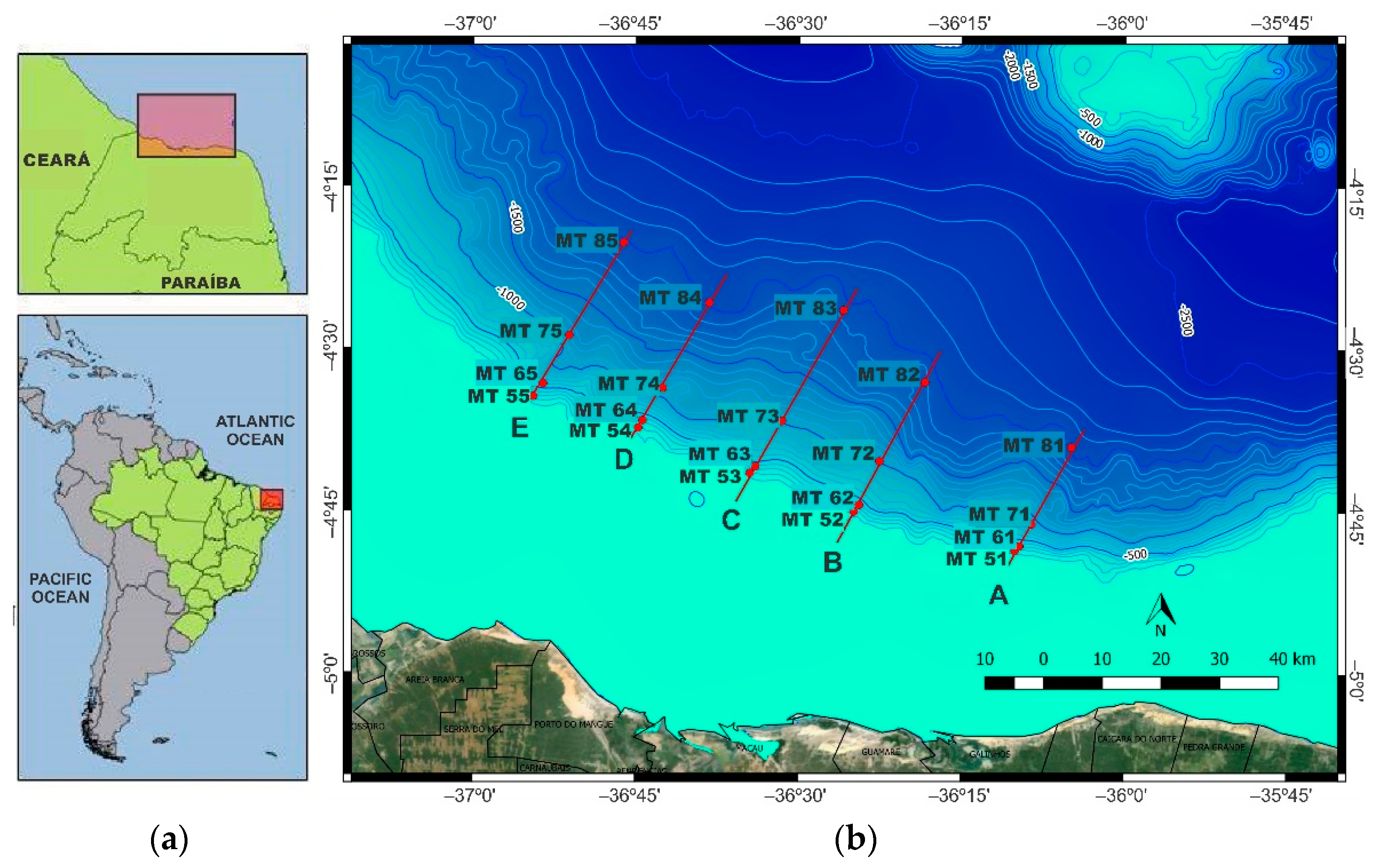
2. Study Area
3. Materials and Methods
3.1. Sediment Sampling
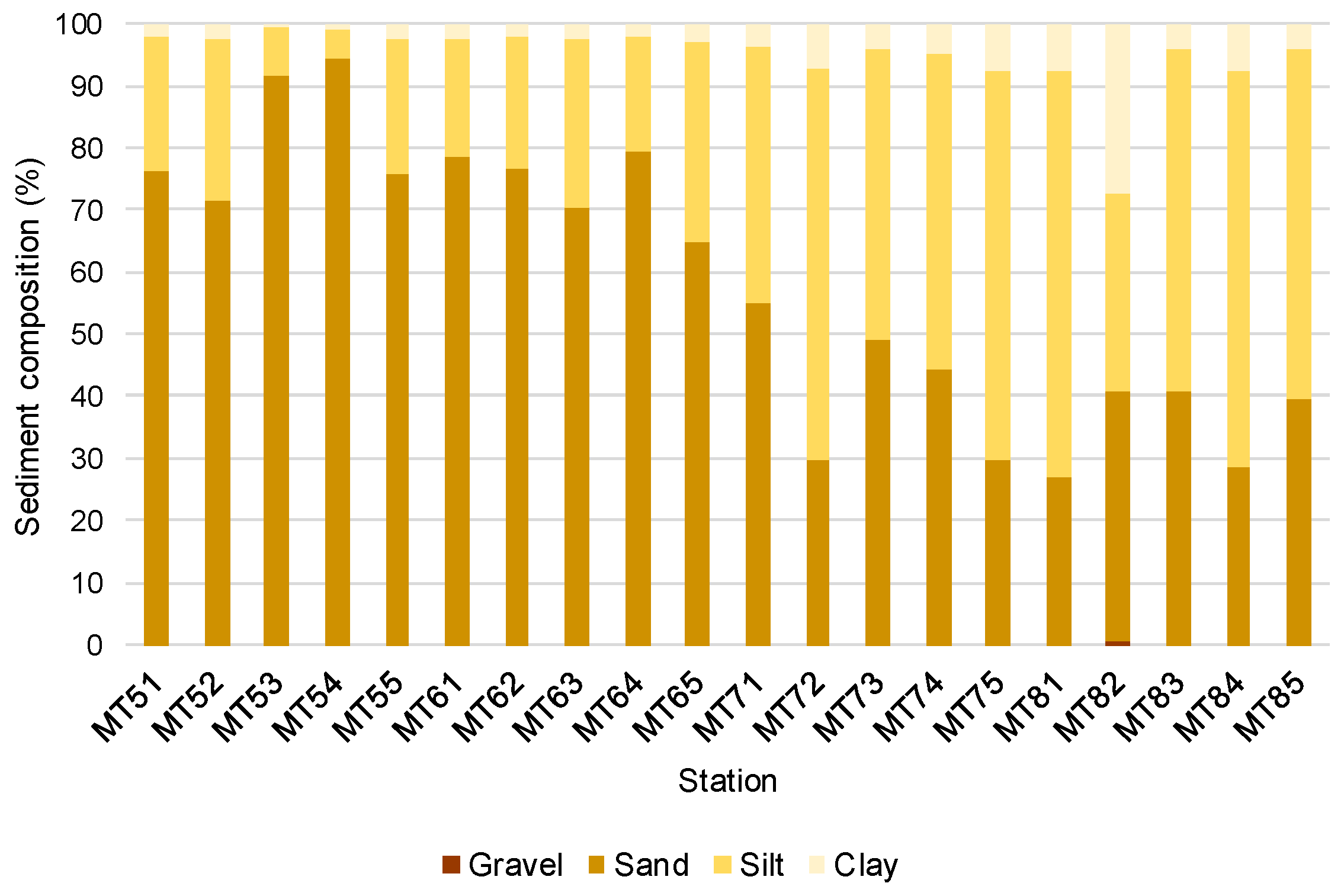
3.2. Granulometric Analysis
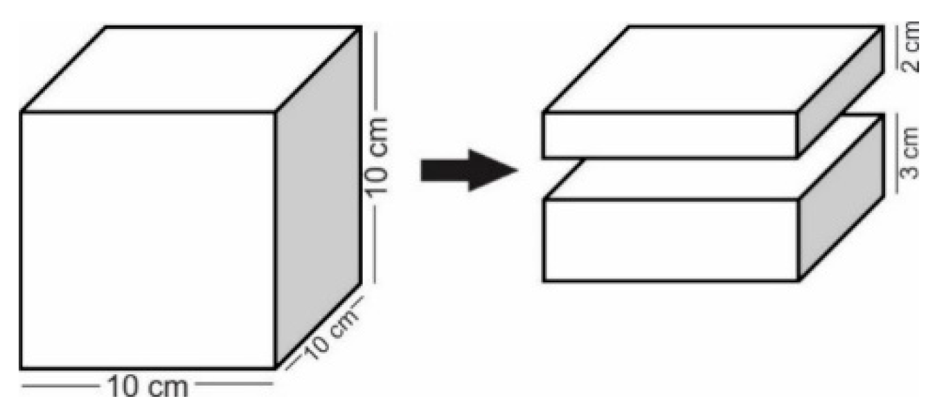
3.3. Foraminifera—Samples Processing
3.4. Statistical Treatment
4. Results
4.1. Abiotic Data
4.2. Foraminifera
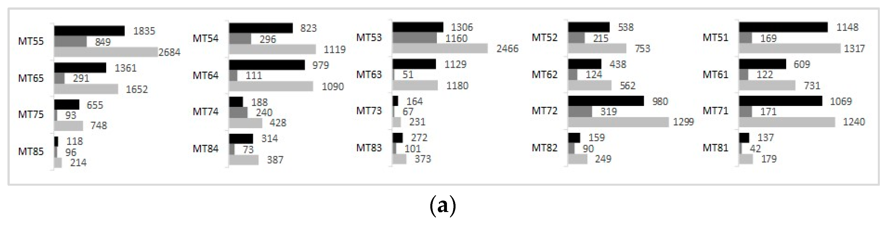
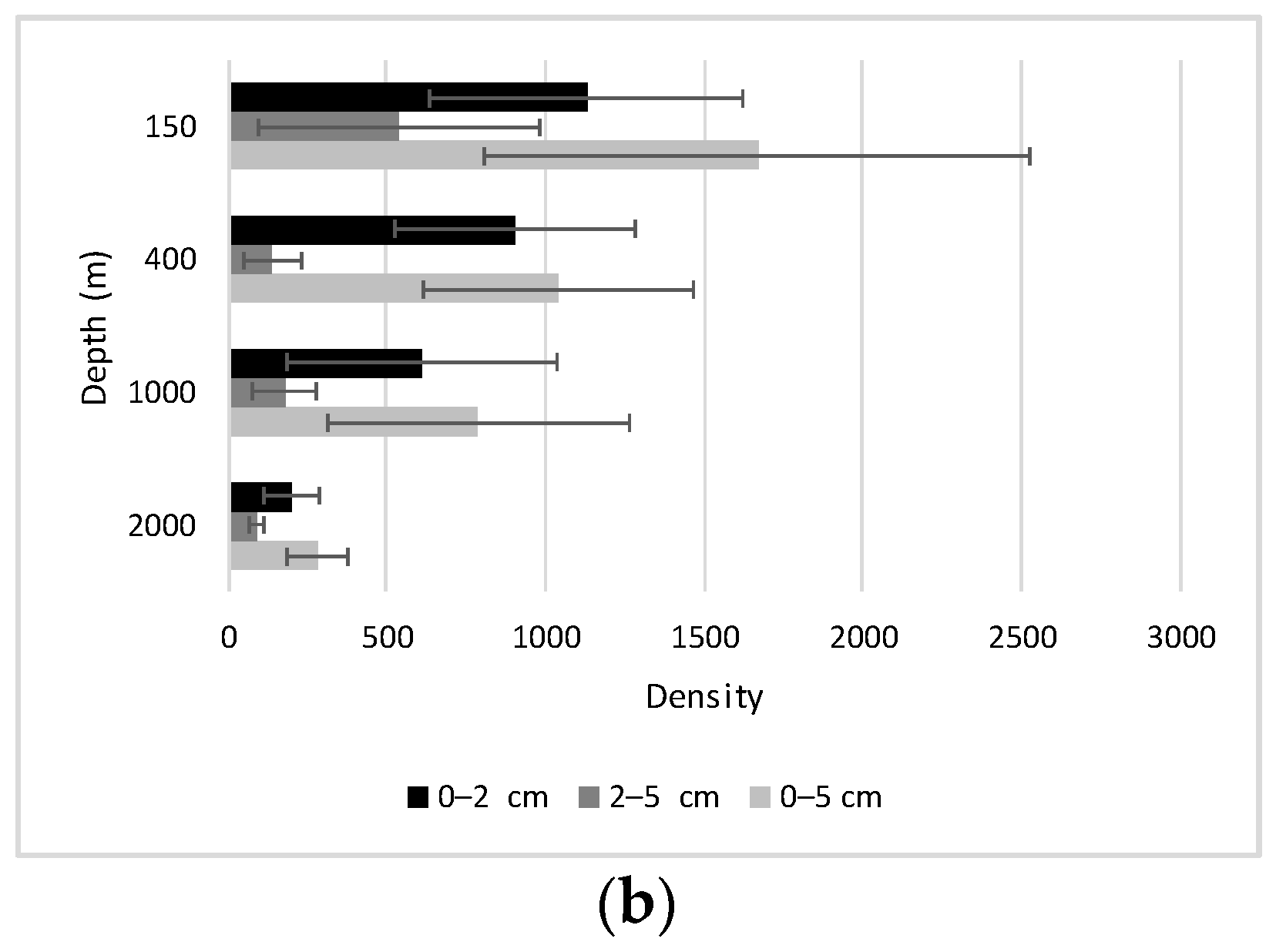
4.2.1. Density
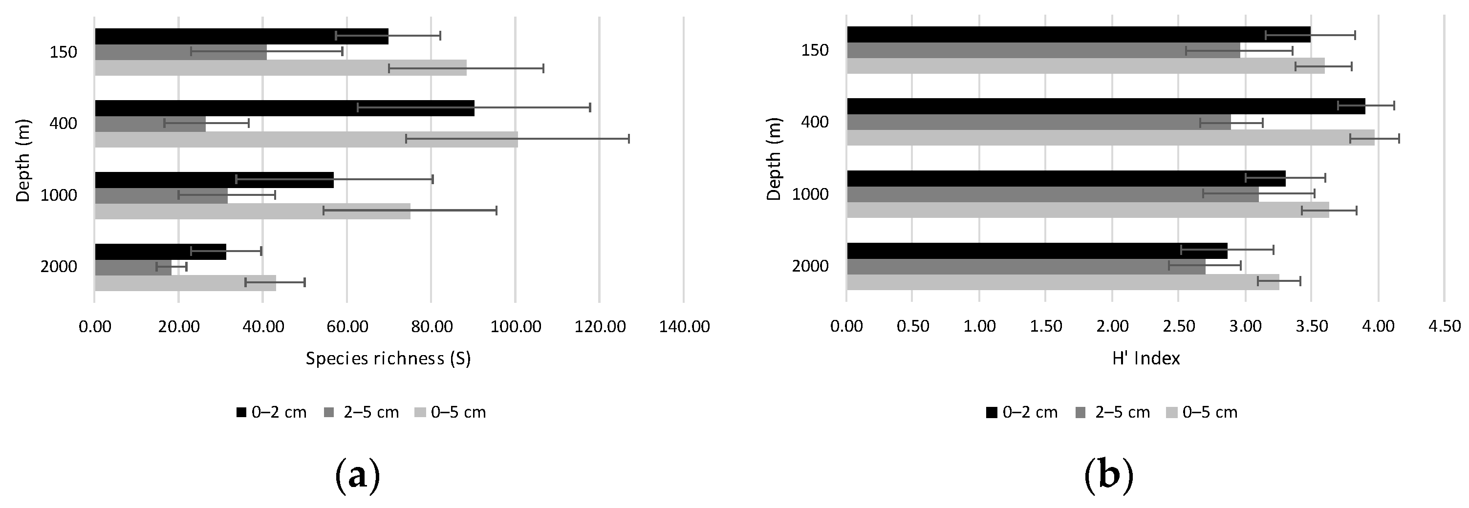
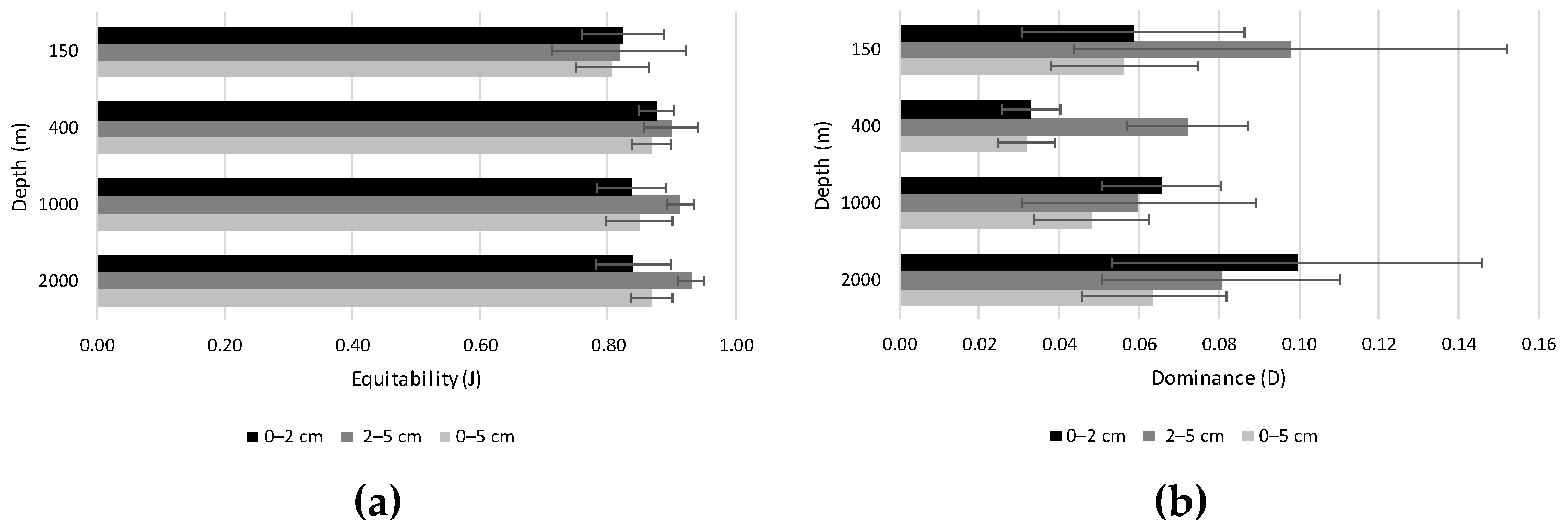
4.2.2. Diversity
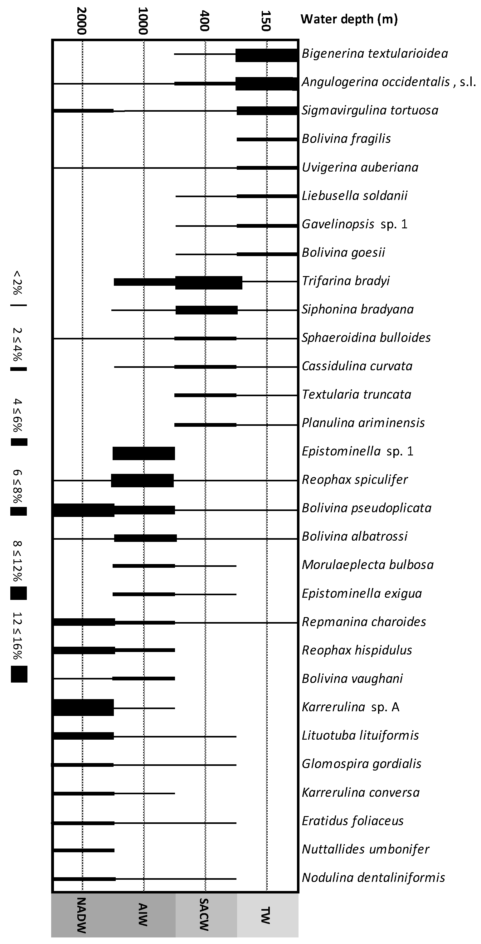
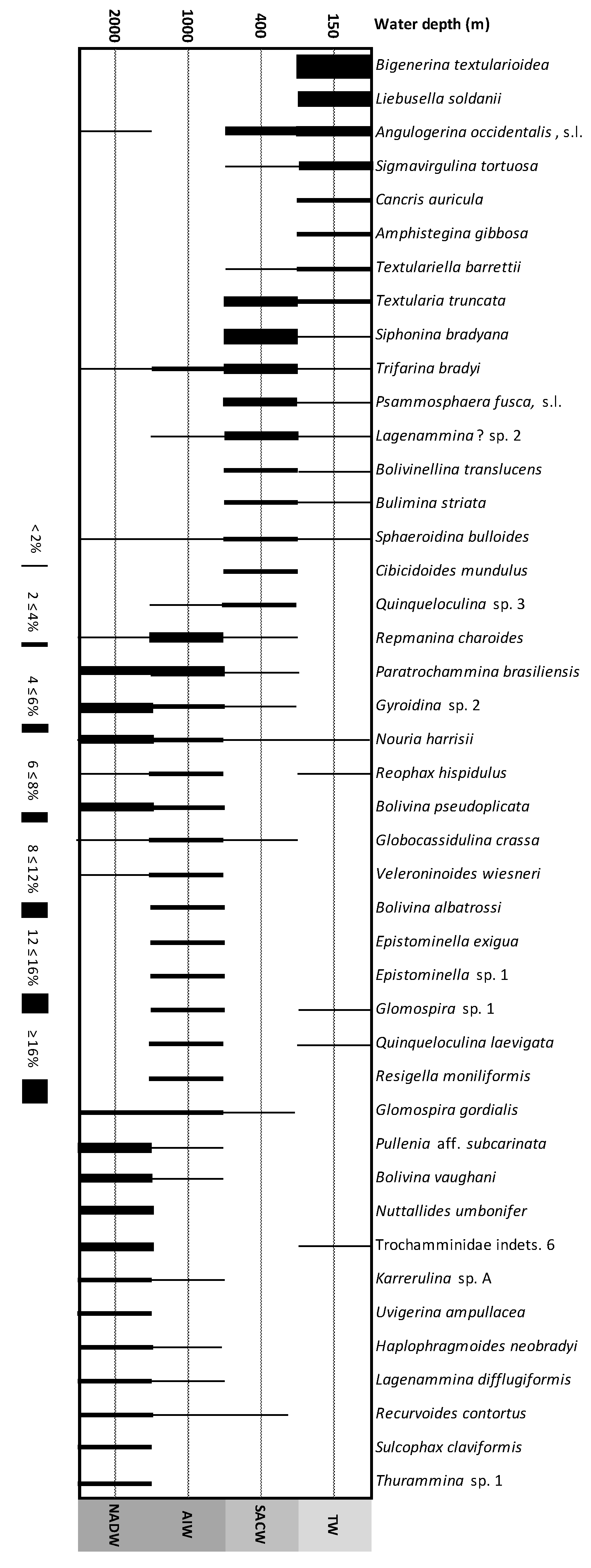
4.2.3. Composition of Assemblages: Major Taxa
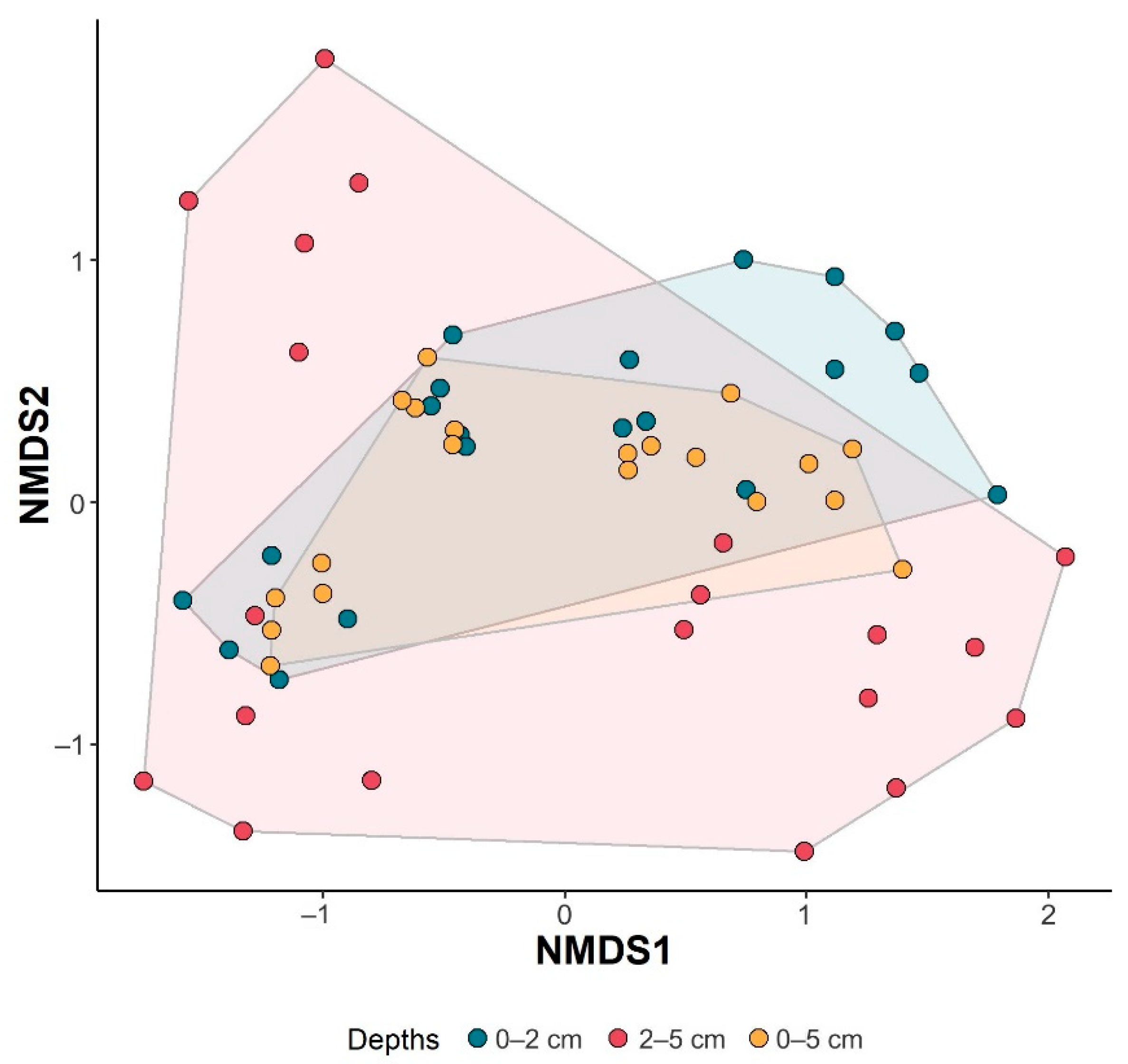
4.2.4. Comparison of Assemblages
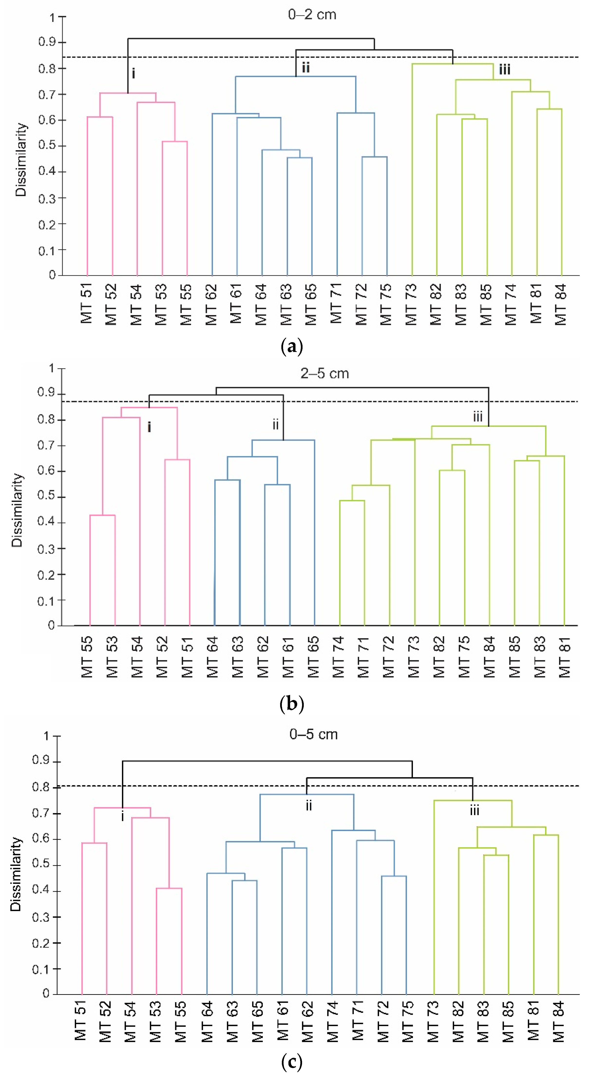
4.2.5. Cluster Analysis
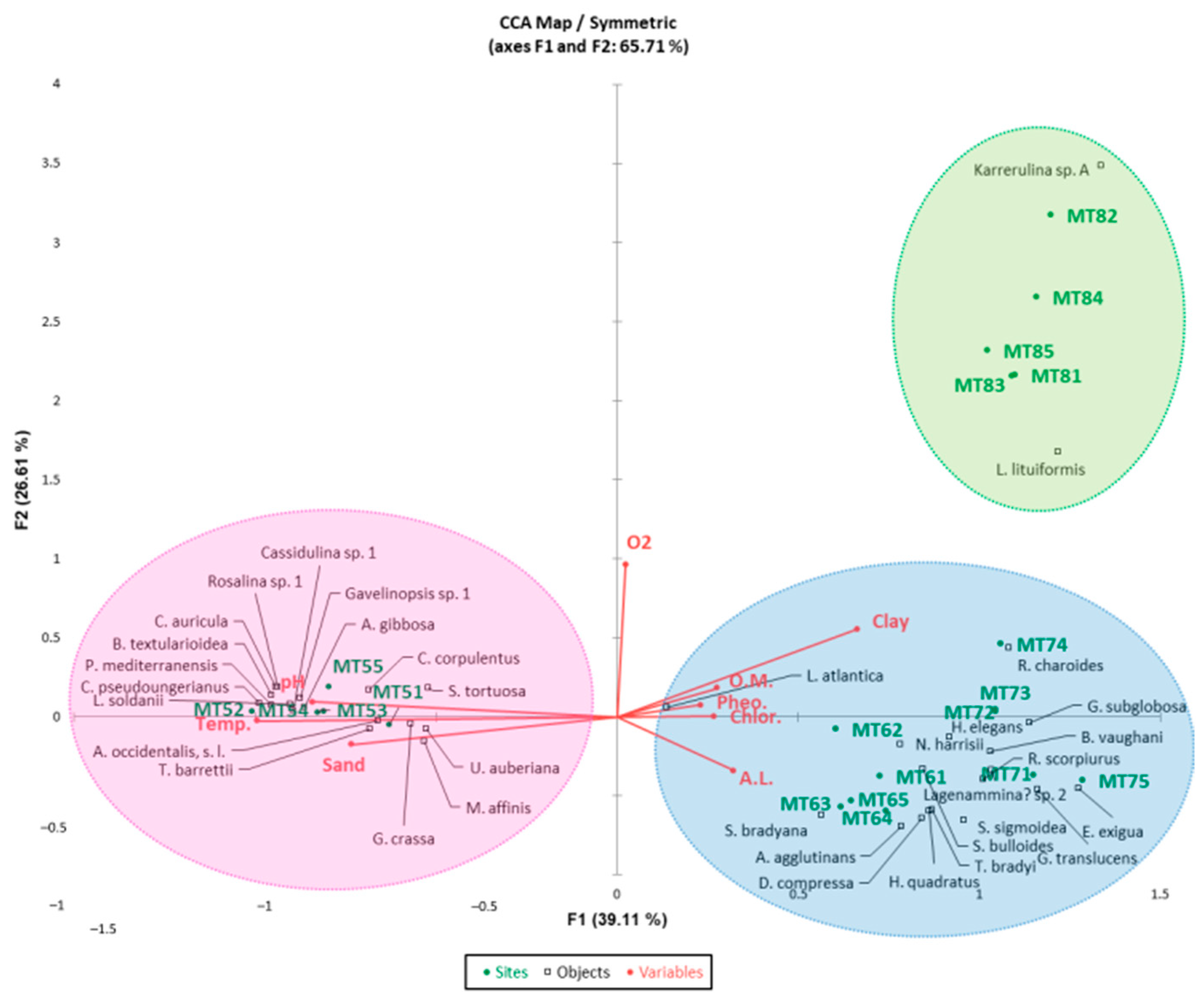
4.2.6. Canonical Correspondence Analysis
5. Discussion
6. Conclusions
Supplementary Materials
Author Contributions
Funding
Institutional Review Board Statement
Informed Consent Statement
Data Availability Statement
Acknowledgments
Conflicts of Interest
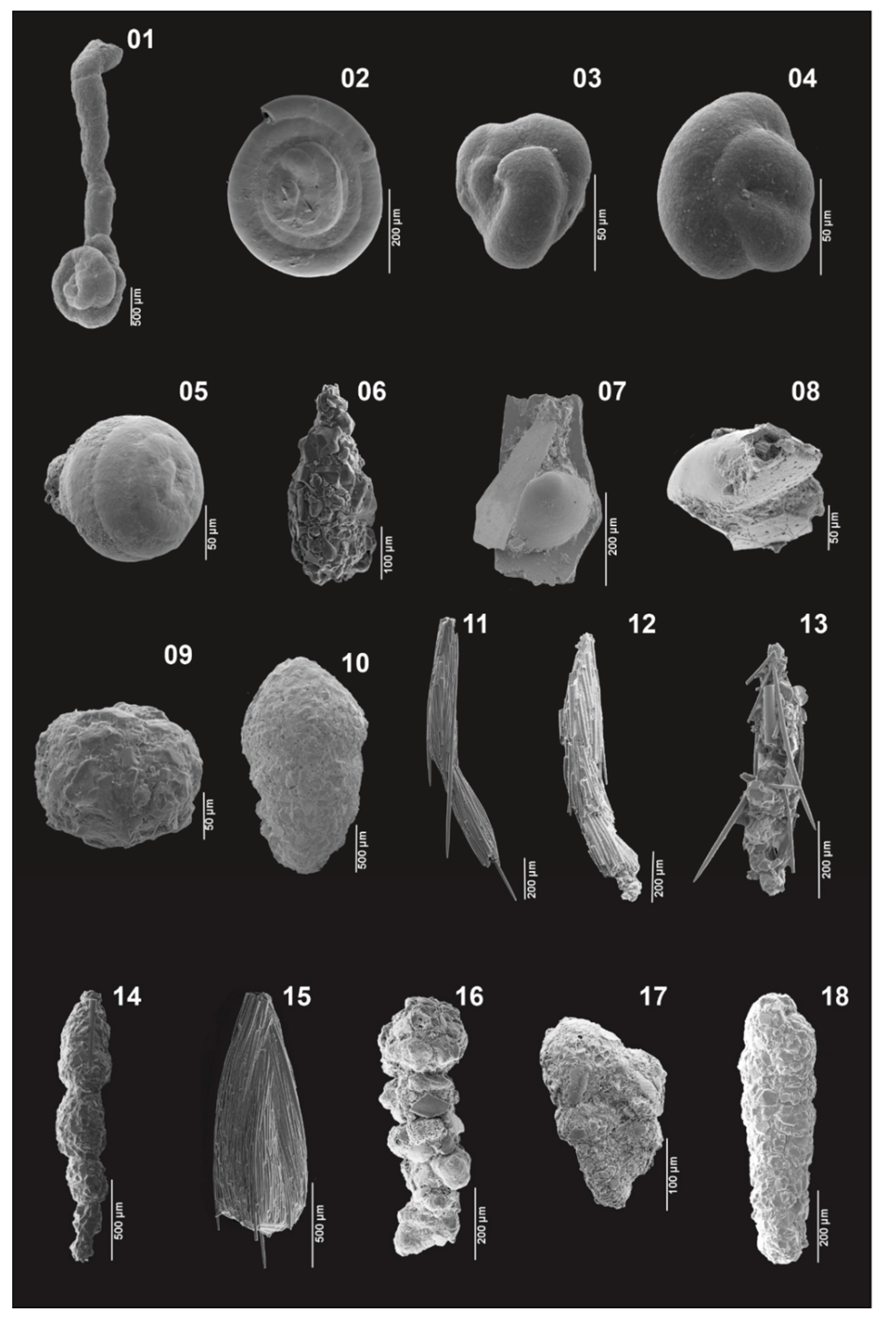
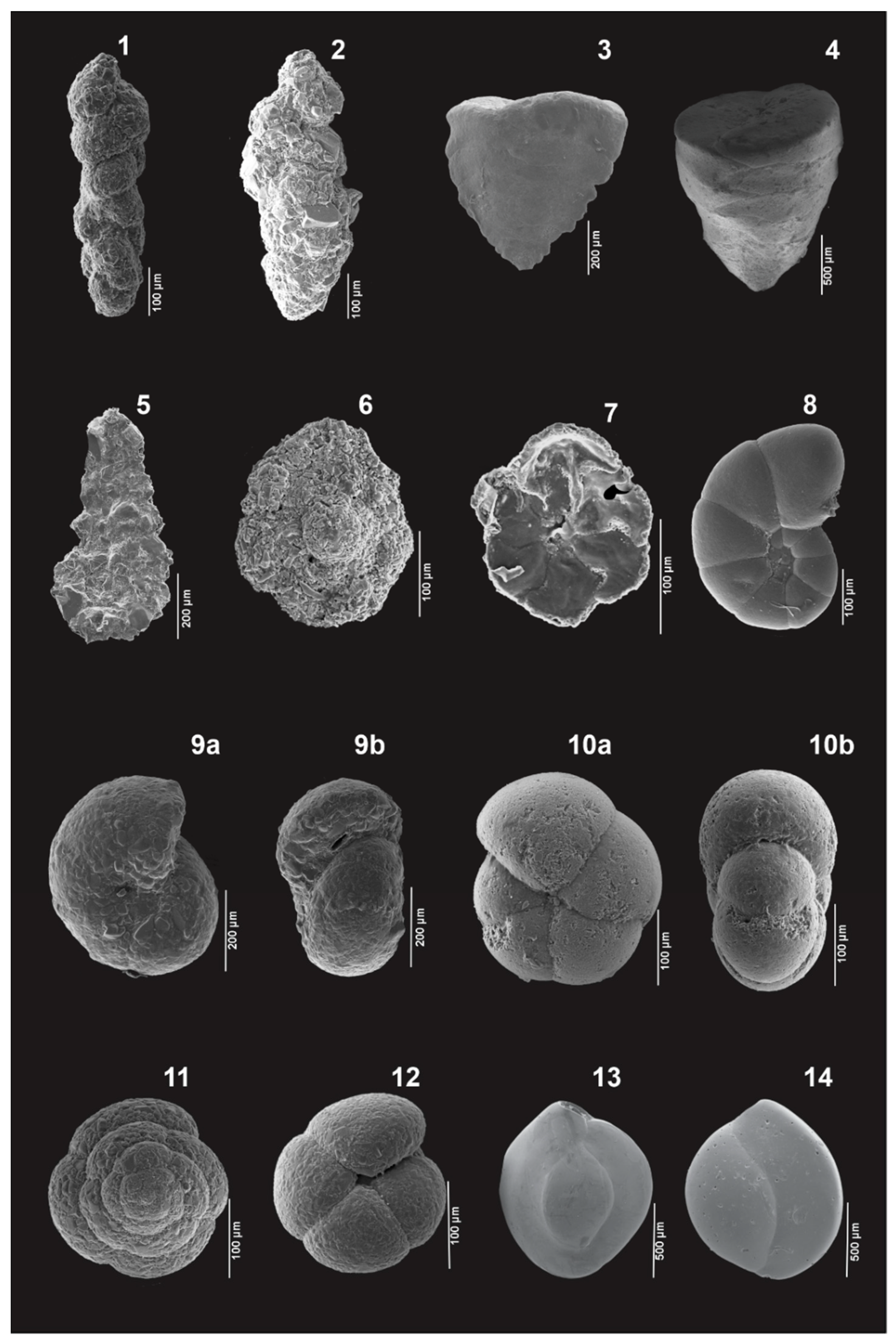
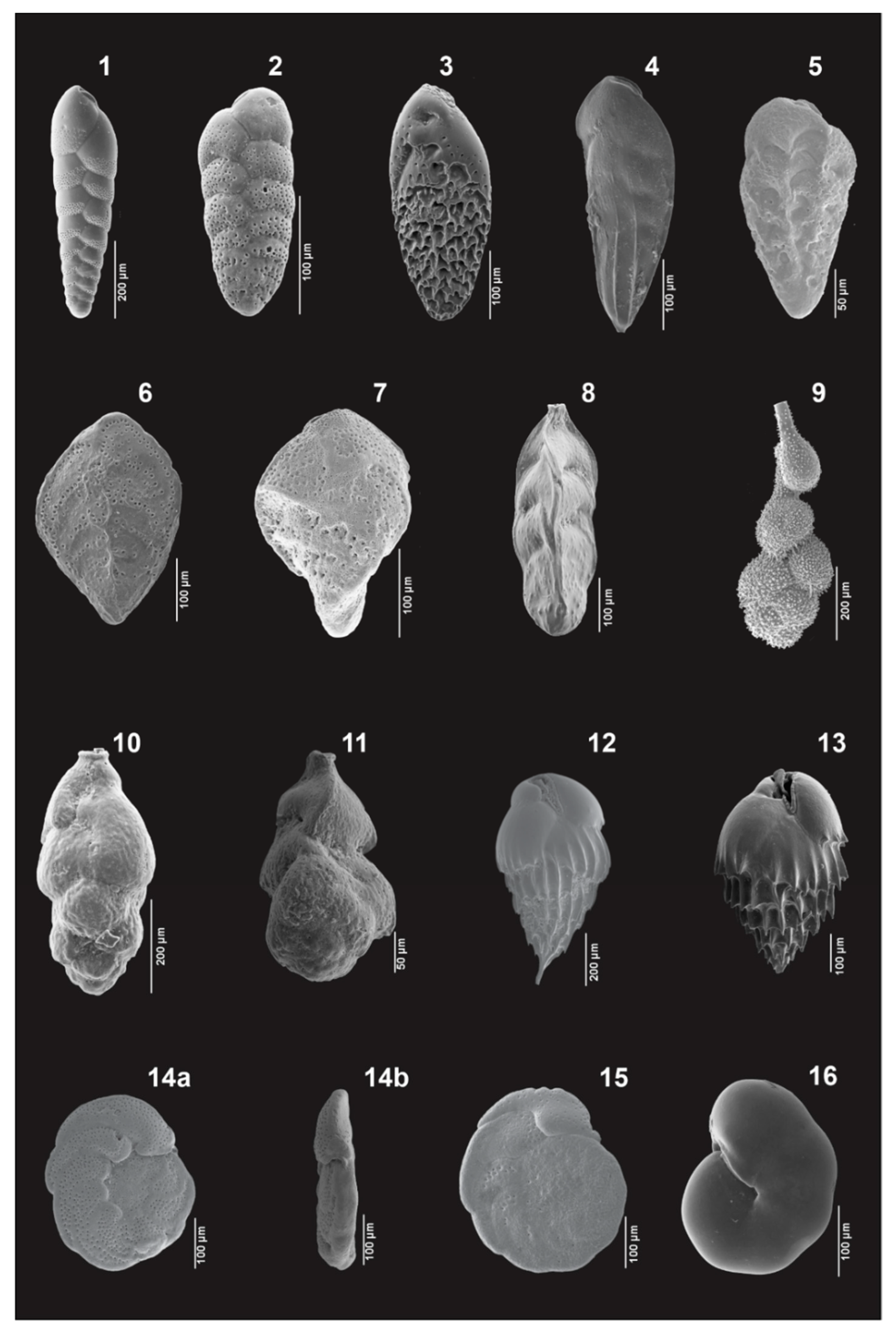
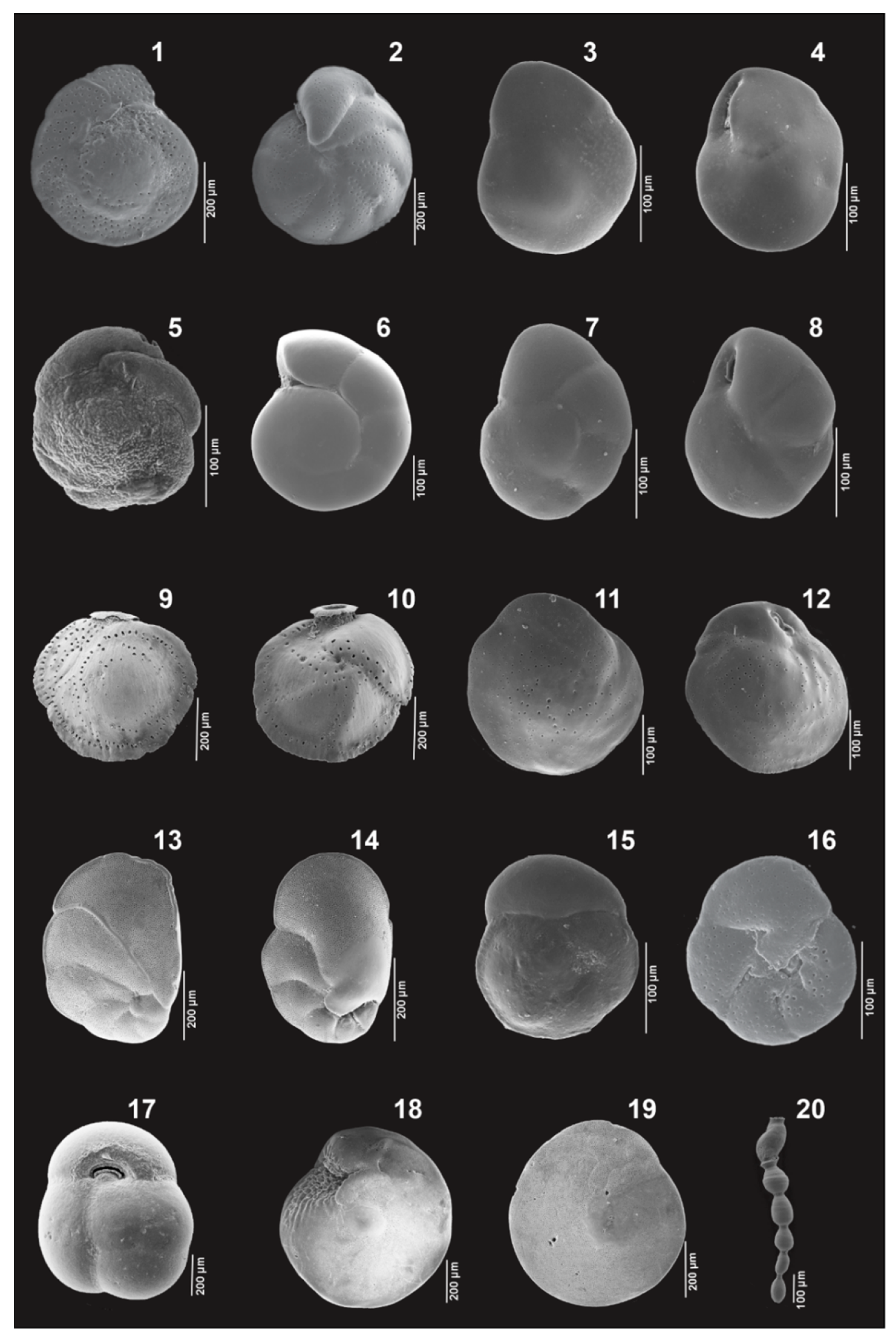
Appendix A. Plates


References
- Alve, E. Benthic Foraminiferal Responses to Estuarine Pollution: A Review. J. Foraminifer. Res. 1995, 25, 190–203. [Google Scholar] [CrossRef]
- Armynot du Châtelet, E.; Gebhardt, K.; Langer, M.R. Coastal Pollution Monitoring: Foraminifera as Tracers of Environmental Perturbation in the Port of Boulogne-Sur-Mer (Northern France). Neues Jahrb. Geol. Palaontol. Abh. 2011, 262, 91–116. [Google Scholar] [CrossRef]
- Bouchet, V.M.P.; Alve, E.; Rygg, B.; Telford, R.J. Benthic Foraminifera Provide a Promising Tool for Ecological Quality Assessment of Marine Waters. Ecol. Indic. 2012, 23, 66–75. [Google Scholar] [CrossRef]
- Martins, M.V.A.; Yamashita, C.; de Mello e Sousa, S.H.; Koutsoukos, E.A.M.; Disaró, S.T.; Debenay, J.P.; Duleba, W. Response of Benthic Foraminifera to Environmental Variability: Importance of Benthic Foraminifera in Monitoring Studies; Bachari Fouzia, H., Ed.; IntechOpen: London, UK, 2019; ISBN 978-1-83880-811-2. [Google Scholar]
- Sousa, S.H.M.; Yamashita, C.; Semensatto, D.L.; Santarosa, A.C.A.; Iwai, F.S.; Omachi, C.Y.; Disaró, S.T.; Martins, M.V.A.; Barbosa, C.F.; Bonetti, C.H.C.; et al. Opportunities and Challenges in Incorporating Benthic Foraminifera in Marine and Coastal Environmental Biomonitoring of Soft Sediments: From Science to Regulation and Practice. J. Sediment. Environ. 2020, 5, 257–265. [Google Scholar] [CrossRef]
- Schönfeld, J.; Alve, E.; Geslin, E.; Jorissen, F.; Korsun, S.; Spezzaferri, S.; Abramovich, S.; Almogi-Labin, A.; Armynot du Chatelet, E.; Barras, C.; et al. The FOBIMO (FOraminiferal BIo-MOnitoring) Initiative-Towards a Standardised Protocol for Soft-Bottom Benthic Foraminiferal Monitoring Studies. Mar. Micropaleontol. 2012, 94–95, 1–13. [Google Scholar] [CrossRef]
- Jorissen, F.J. Benthic foraminiferal microhabitats below the sediment-water interface. In Modern Foraminifera; Springer: Dordrecht, The Netherlands, 1999; pp. 161–179. [Google Scholar]
- Linke, P.; Lutze, G.F. Microhabitat Preferences of Benthic Foraminifera-a Static Concept or a Dynamic Adaptation to Optimize Food Acquisition? Mar. Micropaleontol. 1993, 20, 215–234. [Google Scholar] [CrossRef] [Green Version]
- Corliss, B.H. Morphology and Microhabitat Preferences of Benthic Foraminifera from the Northwest Atlantic Ocean. Mar. Micropaleontol. 1991, 17, 195–236. [Google Scholar] [CrossRef]
- Gooday, A.J. Meiofaunal Foraminiferans from the Bathyal Porcupine Seabight (Northeast Atlantic): Size Structure, Standing Stock, Taxonomic Composition, Species Diversity and Vertical Distribution in the Sediment. Deep Sea Res. Part A Oceanogr. Res. Pap. 1986, 33. [Google Scholar] [CrossRef]
- Fontanier, C.; Jorissen, F.J.; Chailloua, G.; David, C.; Anschutz, P.; Lafon, V. Seasonal and Interannual Variability of Benthic Foraminiferal Faunas at 550 m Depth in the Bay of Biscay. Deep Res. Part I Oceanogr. Res. Pap. 2003, 50, 457–494. [Google Scholar] [CrossRef]
- Heinz, P.; Hemleben, C. Regional and Seasonal Variations of Recent Benthic Deep-Sea Foraminifera in the Arabian Sea. Deep Res. Part I Oceanogr. Res. Pap. 2003, 50, 435–447. [Google Scholar] [CrossRef]
- Szarek, R.; Nomaki, H.; Kitazato, H. Living Deep-Sea Benthic Foraminifera from the Warm and Oxygen-Depleted Environment of the Sulu Sea. Deep Res. Part II Top. Stud. Oceanogr. 2007, 54, 145–176. [Google Scholar] [CrossRef]
- Fontanier, C.; Jorissen, F.J.; Lansard, B.; Mouret, A.; Buscail, R.; Schmidt, S.; Kerhervé, P.; Buron, F.; Zaragosi, S.; Hunault, G.; et al. Live Foraminifera from the Open Slope between Grand Rhône and Petit Rhône Canyons (Gulf of Lions, NW Mediterranean). Deep Res. Part I Oceanogr. Res. Pap. 2008, 55, 1532–1553. [Google Scholar] [CrossRef] [Green Version]
- Mojtahid, M.; Griveaud, C.; Fontanier, C.; Anschutz, P.; Jorissen, F.J. Les Foraminifères Benthiques Vivants Le Long d’un Transect Bathymétrique (140-4800m) Dans Le Golfe de Gascogne (Atlantique NE). Rev. Micropaleontol. 2010, 53, 139–162. [Google Scholar] [CrossRef] [Green Version]
- Fontanier, C.; Metzger, E.; Waelbroeck, C.; Jouffreau, M.; Lefloch, N.; Jorissen, F.; Etcheber, H.; Bichon, S.; Chabaud, G.; Poirier, D.; et al. Live (Stained) Benthic Foraminifera off Walvis Bay, Namibia: A Deep-Sea Ecosystem under the Influence of Bottom Nepheloid Layers. J. Foraminifer. Res. 2013, 43, 55–71. [Google Scholar] [CrossRef] [Green Version]
- Fontanier, C.; Garnier, E.; Brandily, C.; Dennielou, B.; Bichon, S.; Gayet, N.; Eugene, T.; Rovere, M.; Grémare, A.; Deflandre, B. Living (Stained) Benthic Foraminifera from the Mozambique Channel (Eastern Africa): Exploring Ecology of Deep-Sea Unicellular Meiofauna. Deep Res. Part I Oceanogr. Res. Pap. 2016, 115, 159–174. [Google Scholar] [CrossRef] [Green Version]
- Singh, D.P.; Saraswat, R.; Kaithwar, A. Changes in Standing Stock and Vertical Distribution of Benthic Foraminifera along a Depth Gradient (58–2750 m) in the Southeastern Arabian Sea. Mar. Biodivers. 2018, 48, 73–88. [Google Scholar] [CrossRef]
- Licari, L.; Mackensen, A. Benthic Foraminifera off West Africa (1° N to 32° S): Do Live Assemblages from the Topmost Sediment Reliably Record Environmental Variability? Mar. Micropaleontol. 2005, 55, 205–233. [Google Scholar] [CrossRef]
- Almeida, N.M.; Vital, H.; Gomes, M.P. Morphology of Submarine Canyons along the Continental Margin of the Potiguar Basin, NE Brazil. Mar. Pet. Geol. 2015, 68, 307–324. [Google Scholar] [CrossRef]
- Gomes, M.P.; Vital, H. Revisão Da Compartimentação Geomorfológica Da Plataforma Continental Norte Do Rio Grande Do Norte, Brasil. Rev. Bras. Geociênc. 2010, 40, 321–329. [Google Scholar] [CrossRef] [Green Version]
- Stramma, L.; England, M. On the Water Masses and Mean Circulation of the South Atlantic Ocean. J. Geophys. Res. Ocean. 1999, 104, 20863–20883. [Google Scholar] [CrossRef]
- Silveira, I.C.A.; Schmidt, A.C.K.; Campos, E.J.D.; Godoi, S.S.; Ikeda, Y. A Corrente Do Brasil Ao Largo Da Costa Leste Brasileira. Braz. J. Oceanogr. 2000, 48, 171–183. [Google Scholar] [CrossRef]
- Marin, F.D.O. A Subcorrente Norte do Brasil Ao Largo da Costa do Nordeste. Master’s Thesis, Universidade de São Paulo, São Paulo, Brazil, 2009. [Google Scholar]
- Silveira, I.C.A.; Flierl, G.R. Eddy Formation in 2 1/2-Layer, Quasigeostrophic Jets. J. Phys. Oceanogr. 2002, 32, 729–745. [Google Scholar] [CrossRef]
- Krelling, A.P.M. A Estrutura Vertical dos Vórtices da Corrente Norte do Brasil. Master’s Thesis, Universidade Federal do Rio de Janeiro, Rio de Janeiro, Brazil, 2010. [Google Scholar]
- Testa, V.; Bosence, D.W.J. Carbonate-Siliciclastic Sedimentation on a High-Energy, Ocean-Facing, Tropical Ramp, NE Brazil. Geol. Soc. Spec. Publ. 1998, 149, 55–71. [Google Scholar] [CrossRef]
- Krelling, A.P.M.; Silveira, I.C.A.; Polito, P.S.; Gangopadhyay, A.; Martins, R.P.; Lima, J.A.M.; Marin, F.O. A Newly Observed Quasi-Stationary Subsurface Anticyclone of the North Brazil Undercurrent at 4° S: The Potiguar Eddy. J. Geophys. Res. Ocean. 2020, 125, 1–16. [Google Scholar] [CrossRef]
- Walton, W.R. Techniques for Recognition of Living Foraminifera. Contrib. Cushman Found. Foraminifer. Res. 1952, 3, 56–60. [Google Scholar]
- Folk, R.L. Petrology of Sedimentary Rocks; Hemphill Publishing Company: Austin, TX, USA, 1968; ISBN 0914696149. [Google Scholar]
- Ellis, B.F.; Messina, A.R. Catalogue of Foraminifera; Micropaleontology Press, American Museum of Natural History: New York, NY, USA, 1940. [Google Scholar]
- Loeblich, A.R.; Tappan, H. Foraminiferal Genera and Their Classification; Van Nostrand Reinhold Company: New York, NY, USA, 1987. [Google Scholar]
- Loeblich, A.R.; Tappan, H. Foraminifera of the Sahul Shelf and Timor Sea; Special Publication No. 31; Cushman Foundation for Foraminiferal Research: Lawrence, KS, USA, 1994. [Google Scholar]
- Hottinger, L.; Halicz, E.; Reiss, Z. Recent Foraminifera from the Gulf of Aqaba, Red Sea; Slovenska Akademija Znanosti in Umetnosti: Ljubljana, Slovenia, 1993. [Google Scholar]
- Kaminski, M.A. The Year 2000 Classification of the agglutinated foraminifera. In Proceedings of the Sixth International Workshop on Agglutinated Foraminifera, Prague, Czech Republic, 1–7 September 2001; Bubík, M., Kaminski, M.A., Eds.; Grzybowski Foundation Special Publication, 2004; Volume 8, pp. 237–255. Available online: http://gf.tmsoc.org/Documents/Library/2000.pdf (accessed on 10 December 2020).
- Hayward, B.W.; Grenfell, H.R.; Sabaa, A.T.; Neil, H.; Buzas, M.A. Recent New Zealand Deep-Water Benthic Foraminifera: Taxonomy, Ecologic Distribution, Biogeography, and Use in Paleoenvironmental Assessment; GNS Science: Lower Hutt, New Zealand, 2010; ISBN 9780478197778 (pbk.). [Google Scholar]
- Debenay, J.P. A Guide to 1000 Foraminifera from Southwestern Pacific New Caledonia; French National Museum Natural History: Marseille, France, 2012. [Google Scholar]
- Kaminski, M.A.; Cetean, C.G. A Catalogue of Agglutinated Foraminiferal Genera. Unpublished.
- Efron, B. Bootstrap Methods: Another Look at the Jackknife. Ann. Stat. 1979, 7, 1–26. [Google Scholar] [CrossRef]
- Magurran, A.E. Medindo a Diversidade Biológica; Editora UFPR: Curitiba, Brazil, 2013; Volume 1, ISBN 9788573352788. [Google Scholar]
- Chao, A.; Gotelli, N.J.; Hsieh, T.C.; Sander, E.L.; Ma, K.H.; Colwell, R.K.; Ellison, A.M. Rarefaction and Extrapolation with Hill Numbers: A Framework for Sampling and Estimation in Species Diversity Studies. Ecol. Monogr. 2014, 84, 45–67. [Google Scholar] [CrossRef] [Green Version]
- R Core Team R. A Language and Environment for Statistical Computing; R Foundation for Statistical Computing: Vienna, Austria, 2018. [Google Scholar]
- Hsieh, T.C.; Ma, K.H.; Chao, A. INEXT: An R Package for Rarefaction and Extrapolation of Species Diversity (Hill Numbers). Methods Ecol. Evol. 2016, 7, 1451–1456. [Google Scholar] [CrossRef]
- Clarke, K. Non-Parametric Multivariate Analyses of Changes in Community Structure. Aust. J. Ecol. 1993, 18, 117–143. [Google Scholar] [CrossRef]
- Oksanen, A.J.; Blanchet, F.G.; Friendly, M.; Kindt, R.; Legendre, P.; Mcglinn, D.; Minchin, P.R.; Hara, R.B.O.; Simpson, G.L.; Solymos, P.; et al. Vegan: Community Ecology Package 2018. Available online: https://cran.r-project.org/web/packages/vegan/index.html (accessed on 10 February 2021).
- Salazar, G. EcolUtils R Package 2021. Available online: https://github.com/GuillemSalazar/EcolUtils (accessed on 10 February 2021).
- XLSTAT Data Analysis and Statistical Solution for Microsoft Excel 2016. Available online: https://www.xlstat.com/en/ (accessed on 20 April 2021).
- Dufrene, M.; Legendre, P. Species Assemblages and Indicator Species: The Need for a Flexible Assymmetrical Aproach. Ecol. Monogr. 1997, 67, 345–366. [Google Scholar] [CrossRef]
- Hammer, Ø.; Harper, D.A.T.; Ryan, P.D. Past: Paleontological Statistics Software Package for Education and Data Analysis. Palaeontol. Electron. 2001, 4, 1–9. [Google Scholar]
- Vital, H.; Gomes, M.P.; Tabosa, W.F.; Frazão, E.P.; Santos, C.L.A.; Plácido Júnior, J.S. Characterization of the Brazilian Continental Shelf Adjacent to Rio Grande Do Norte State, Ne Brazil. Braz. J. Oceanogr. 2010, 58, 43–54. [Google Scholar] [CrossRef]
- Buzas, M.A.; Hayek, L.-A.C.; Jett, J.A.; Reed, S.A. Pulsating Patches History and Analyses of Spatial, Seasonal, and Yearly Distribution of Living Benthic Foraminifera; Smithsonian Institution Scholarly Press: Washington, DC, USA, 2015. [Google Scholar]
- Schmiedl, G.; Mackensen, A.; Müller, P.J. Recent Benthic Foraminifera from the Eastern South Atlantic Ocean: Dependence on Food Supply and Water Masses. Mar. Micropaleontol. 1997, 32, 249–287. [Google Scholar] [CrossRef]
- Hayward, B.W.; Grenfell, H.R.; Sabaa, A.T.; Neil, H.L. Factors Influencing the Distribution of Subantarctic Deep-Sea Benthic Foraminifera, Campbell and Bounty Plateaux, New Zealand. Mar. Micropaleontol. 2007, 62, 141–166. [Google Scholar] [CrossRef]
- Burone, L.; Sousa, S.H.M.; de Mahiques, M.M.; Valente, P.; Ciotti, A.; Yamashita, C. Benthic Foraminiferal Distribution on the Southeastern Brazilian Shelf and Upper Slope. Mar. Biol. 2011, 158, 159–179. [Google Scholar] [CrossRef]
- Phipps, M.; Jorissen, F.; Pusceddu, A.; Bianchelli, S.; De Stigter, H. Live Benthic Foraminiferal Faunas along a Bathymetrical Transect (282-4987 M) on the Portuguese Margin (Ne Atlantic). J. Foraminifer. Res. 2012, 42, 66–81. [Google Scholar] [CrossRef] [Green Version]
- Fiorini, F. Recent Benthic Foraminifera from the Caribbean Continental Slope and Shelf off West of Colombia. J. S. Am. Earth Sci. 2015, 60, 117–128. [Google Scholar] [CrossRef]
- Bernhard, J.M. Distinguishing Live from Dead Foraminifera: Methods Review and Proper Applications. Micropaleontology 2000, 46, 38–46. [Google Scholar]
- Sen Gupta, B.K.; Platon, E.; Bernhard, J.M.; Aharon, P. Foraminiferal Colonization of Hydrocarbon-Seep Bacterial Mats and Underlying Sediment, Gulf of Mexico Slope. J. Foraminifer. Res. 1997, 27, 292–300. [Google Scholar] [CrossRef]
- Murray, J.W. Ecology and Applications of Benthic Foraminifera; Cambridge University Press: New York, NY, USA, 2006; ISBN 9780511535529. [Google Scholar]
- Buzas, M.A.; Gibson, T.G. Species Diversity: Benthonic Foraminifera in Western North Atlantic. Sci. New Ser. 1969, 163, 72–75. [Google Scholar] [CrossRef]
- Gibson, T.G.; Buzas, M.A. Species Diversity: Patterns in Modern and Miocene Foraminifera of the Eastern Margin of North America. Bull. Geol. Soc. Am. 1973, 84, 217–238. [Google Scholar] [CrossRef]
- Disaró, S.T.; Watanabe, S.; Totah, V.; Barbosa, V.P.; Koutsoukos, E.A.M.; Itice, I.; Pupo, D.V.; Chiaverini, A.P.; Foraminíferos, V.I.M. Relatório Integrador do Programa de Monitoramento Ambiental da Bacia Potiguar, IBAMA, Inédito (Acesso Restrito); Rocha, M., Ed.; IBAMA: Rio de Janeiro, Brazil, 2006; pp. 1–85.
- Lavrado, H.P.; Disaró, S.T.; Esteves, A.M.; da Fonsêca-Genevois, V.; de Mello e Sousa, S.H.; Omena, E.P.; Paranhos, R.; Sallorenzo, I.; Veloso, V.G.; Ribeiro-Ferreira, V.P.; et al. Comunidades bentônicas dos substratos inconsolidados da plataforma e talude continental da Bacia de Campos: Uma visão integrada entre seus componentes e suas relações com o ambiente. In Ambiente Bentônico; Falcão, A.P.C., Lavrado, H., Eds.; Elsevier Habitats: Rio de Janeiro, Brazil, 2017; pp. 307–352. [Google Scholar]
- Krelling, A.P.M.; Gangopadhyay, A.; Silveira, I.; Vilela-Silva, F. Development of a Feature-Oriented Regional Modelling System for the North Brazil Undercurrent Region (1°–11 °S) and Its Application to a Process Study on the Genesis of the Potiguar Eddy. J. Oper. Oceanogr. 2020, 1–18. [Google Scholar] [CrossRef]
- Mackensen, A.; Fütterer, D.K.; Grobe, H.; Schmiedl, G. Benthic Foraminiferal Assemblages from the Eastern South Atlantic Polar Front Region between 35° and 57° S: Distribution, Ecology and Fossilization Potential. Mar. Micropaleontol. 1993, 22, 33–69. [Google Scholar] [CrossRef]
- Schnitker, D. West Atlantic Abyssal Circulation during the Past 120,000 Years. Nature 1974, 247, 385–387. [Google Scholar] [CrossRef]
- Lohmann, G.P. Abyssal Benthonic Foraminifera as Hydrographic Indicators in the Western South Atlantic Ocean. J. Foraminifer. Res. 1978, 8, 6–34. [Google Scholar] [CrossRef]
- Gooday, A.J. A Response by Benthic Foraminifera to the Deposition of Phytodetritus in the Deep Sea. Nature 1988, 332, 70–73. [Google Scholar] [CrossRef]
- Gooday, A.J. Deep-Sea Benthic Foraminiferal Species Which Exploit Phytodetritus: Characteristic Features and Controls on Distribution. Mar. Micropaleontol. 1993, 22, 187–205. [Google Scholar] [CrossRef]
- Kurbjeweit, F.; Schmiedl, G.; Schiebel, R.; Hemleben, C.; Pfannkuche, O.; Wallmann, K.; Schäfer, P. Distribution, Biomass and Diversity of Benthic Foraminifera in Relation to Sediment. Geochemistry in the Arabian Sea. Deep Sea Res. Part II Top. Stud. Oceanogr. 2000, 47, 2913–2955. [Google Scholar] [CrossRef]
- Gooday, A.J. Epifaunal and Shallow Infaunal Foraminiferal Communities at Three Abyssal NE Atlantic Sites Subject to Differing Phytodetritus Input Regimes. Deep Res. Part I Oceanogr. Res. Pap. 1996, 43, 1395–1421. [Google Scholar] [CrossRef]
- Disaró, S.T.; Aluizio, R.; Ribas, E.R.; Pupo, D.V.; Tellez, I.R.; Watanabe, S.; Totah, V.I.; Koutsoukos, E.A.M. Foraminíferos Bentônicos na plataforma continental da Bacia de Campos. In Ambiente Bentônico: Caracterização Ambiental Regional da Bacia de Campos, Atlântico Sudoeste; Falcão, A.P.C., Lavrado, H.P., Eds.; Elsevier: Rio de Janeiro, Brazil, 2017; pp. 65–110. Available online: https://www.sciencedirect.com/science/article/pii/B9788535272635500047?via%3Dihub (accessed on 20 May 2021).


| Sample | Lat | Long | Depth (m) | Water Mass |
|---|---|---|---|---|
| MT51 | 04°29′10″ | 36°06′02″ | 167 | TW |
| MT52 | 04°27′01″ | 36°14′56″ | 203 | TW |
| MT53 | 04°24′54″ | 36°20′41″ | 133 | TW |
| MT54 | 04°22′23″ | 36°26′51″ | 128 | TW |
| MT55 | 04°20′39″ | 36°32′40″ | 145 | TW |
| MT61 | 04°28′55″ | 36°05′47″ | 400 | SACW |
| MT62 | 04°26′39″ | 36°14′38″ | 422 | SACW |
| MT63 | 04°24′32″ | 36°20′23″ | 394 | SACW |
| MT64 | 04°21′59″ | 36°26′38″ | 409 | SACW |
| MT65 | 04°19′57″ | 36°32′07″ | 408 | SACW |
| MT71 | 04°27′41″ | 36°05′06″ | 998 | AIW |
| MT72 | 04°24′12″ | 36°13′31″ | 1011 | AIW |
| MT73 | 04°22′01″ | 36°18′55″ | 1100 | AIW |
| MT74 | 04°20′11″ | 36°25′31″ | 983 | AIW |
| MT75 | 04°17′17″ | 36°30′41″ | 970 | AIW |
| MT81 | 04°23′26″ | 36°02′55″ | 2010 | NADW |
| MT82 | 04°19′51″ | 36°11′01″ | 1992 | NADW |
| MT83 | 04°15′52″ | 36°15′31″ | 1957 | NADW |
| MT84 | 04°15′28″ | 36°22′57″ | 1983 | NADW |
| MT85 | 04°12′08″ | 36°27′41″ | 2000 | NADW |
| Layer | S | S(est) 95% CI Lower Bound | S(est) 95% CI Upper Bound | Bootstrap | % |
|---|---|---|---|---|---|
| 0–2 cm | 396 | 376 | 416 | 463 | 85.60 |
| 2–5 cm | 228 | 212 | 244 | 271 | 84.26 |
| 0–5 cm | 449 | 428 | 470 | 520 | 86.36 |
Publisher’s Note: MDPI stays neutral with regard to jurisdictional claims in published maps and institutional affiliations. |
© 2021 by the authors. Licensee MDPI, Basel, Switzerland. This article is an open access article distributed under the terms and conditions of the Creative Commons Attribution (CC BY) license (https://creativecommons.org/licenses/by/4.0/).
Share and Cite
Santa-Rosa, L.C.d.C.; Disaró, S.T.; Totah, V.; Watanabe, S.; Guimarães, A.T.B. Living Benthic Foraminifera from the Surface and Subsurface Sediment Layers Applied to the Environmental Characterization of the Brazilian Continental Slope (SW Atlantic). Water 2021, 13, 1863. https://doi.org/10.3390/w13131863
Santa-Rosa LCdC, Disaró ST, Totah V, Watanabe S, Guimarães ATB. Living Benthic Foraminifera from the Surface and Subsurface Sediment Layers Applied to the Environmental Characterization of the Brazilian Continental Slope (SW Atlantic). Water. 2021; 13(13):1863. https://doi.org/10.3390/w13131863
Chicago/Turabian StyleSanta-Rosa, Luciana Cristina de Carvalho, Sibelle Trevisan Disaró, Violeta Totah, Silvia Watanabe, and Ana Tereza Bittencourt Guimarães. 2021. "Living Benthic Foraminifera from the Surface and Subsurface Sediment Layers Applied to the Environmental Characterization of the Brazilian Continental Slope (SW Atlantic)" Water 13, no. 13: 1863. https://doi.org/10.3390/w13131863