
Estimation of Vegetation-Induced Flow Resistance for Hydraulic Computations Using Airborne Laser Scanning Data


Department of Civil and Environmental Engineering, TU Darmstadt, 64289 Darmstadt, Germany
Water 2021, 13(13), 1864; https://doi.org/10.3390/w13131864
Submission received: 1 April 2021
/
Revised: 17 June 2021
/
Accepted: 1 July 2021
/
Published: 4 July 2021
(This article belongs to the Section Hydraulics and Hydrodynamics)
Abstract
:The effect of vegetation in hydraulic computations can be significant. This effect is important for flood computations. Today, the necessary terrain information for flood computations is obtained by airborne laser scanning techniques. The quality and density of the airborne laser scanning information allows for more extensive use of these data in flow computations. In this paper, known methods are improved and combined into a new simple and objective procedure to estimate the hydraulic resistance of vegetation on the flow in the field. State-of-the-art airborne laser scanner information is explored to estimate the vegetation density. The laser scanning information provides the base for the calculation of the vegetation density parameter ωp using the Beer–Lambert law. In a second step, the vegetation density is employed in a flow model to appropriately account for vegetation resistance. The use of this vegetation parameter is superior to the common method of accounting for the vegetation resistance in the bed resistance parameter for bed roughness. The proposed procedure utilizes newly available information and is demonstrated in an example. The obtained values fit very well with the values obtained in the literature. Moreover, the obtained information is very detailed. In the results, the effect of vegetation is estimated objectively without the assignment of typical values. Moreover, a more structured flow field is computed with the flood around denser vegetation, such as groups of bushes. A further thorough study based on observed flow resistance is needed.
1. Introduction
Discharge in watercourses is extremely retarded by vegetation. The flow resistance increases significantly in cases of scarce vegetation with just a few branches per square meter. Dense vegetation drastically reduces the discharge in watercourses.
In most engineering applications, the effect of the vegetation is accounted for by modifying the bed resistance factor, such as the Manning–Strickler coefficient kSt. Despite the strong effect on the discharge, there is not much information available to perform this. The most often used sources of information are maps of land use, aerial photography and perpetration by engineers with experience in this type of model. Guidelines for finding the coefficients are of the type given by Arcement and Schneider [1].
At present, inundation maps are calculated repeatedly using two-dimensional flow models. The guidelines for the determination of the resistance coefficients refer to the maps of land use. In Germany, these maps are available as ATKIS data from governmental agencies. The land use types are converted to values of the bed friction coefficient. This procedure is, however, not very specific, and does not account for the actual vegetation.
Some proposals of using airborne laser scanner data to define vegetation resistance can be found in the literature [2,3,4,5,6]. The method of Järvelä [2] is based on sound hydraulic principles and investigates the resistance of non-submerged vegetation. However, the method needs plant structure parameters, such as diameter, branching and length ratios of the plant parts, as a starting point for the calculation. The values should be taken from the literature. The method is not based on the utilization of the laser scanner information. The method of Straatsma and Babtist [3] is an automated roughness parameterization. However, this method is based on regionalization of the laser scanner information by an iterative cluster merging method. The information is thus highly processed. The information is segmented and classified in land cover usage types. This paper elucidates an automatic procedure to account for the vegetation in the flow computations solely with the use of objectively obtained laser scanning data.
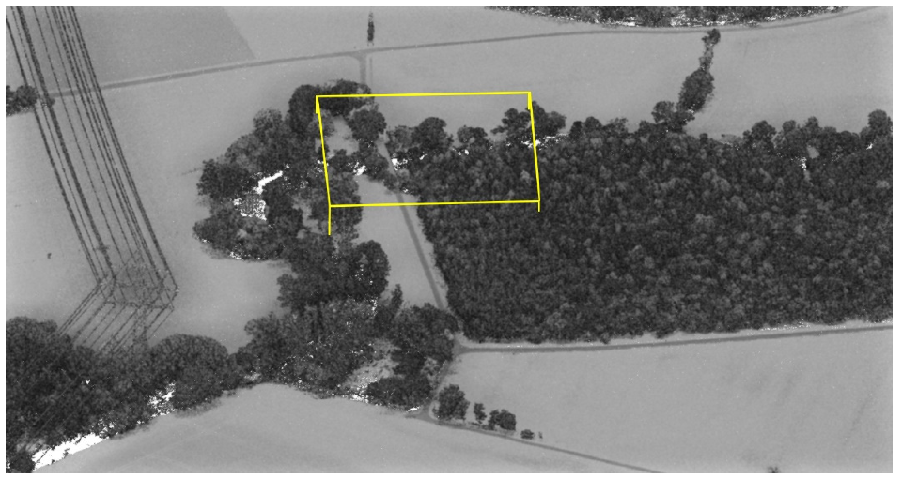
The very high information quality delivered by state-of-the-art airborne laser scanning devices is shown in Figure 1. A short reach of the river Kinzig north-east of the city of Frankfurt in the center of Germany is shown by rendering the intensity of the 3D laser return pulses in greyscale with Cloud Compare. The banklines are full of bushes and trees. Farming fields are well visible in grey while maintenance roads are a bit darker. A woodlot is visible in the right half of the figure. The complete area shown in the figure is often flooded.
Shown is the intensity of the reflections of all points. The Kinzig watercourse itself is left white, because of the lack of back-reflections at the water surface. The vegetation is dark, indicating low intensities of the reflected energy. The ground level is almost bright because of a strong and energetic reflection pulse. The thin-lined box in the center shows the square with an edge length of 50 m, analyzed in more detail in Section 4. The lines in the left part of the figure are high-voltage power lines. Even small bushes are reproduced in amazing detail.
2. Methods for Quantification of Resistance
2.1. Resistance Formulas
Flow resistance induced by obstacles in turbulent flows is governed by Newton’s law:
where Af is the area of the projection of the vegetation parts on a plane normal to the average flow direction, cD—the drag coefficient, —the density of the fluid, —the undisturbed flow velocity vector and h—the water depth. Vegetation is often idealized in laboratory flumes by cylinders standing vertically in the flow. The projected area of the cylinders is the sum of the vertical cross-sections of all individual cylinders, , from the flume floor to the water level. The hydraulic resistance is measured precisely in the laboratory through the water level gradient. In numerous experiments [7,8,9] with different densities of cylindrical obstacles and different Froude and Reynolds numbers, Equation (1) is well established.
For the drag coefficient cD, a constant value of 1.2 is used in this study, even though more accurate values are known from the literature [7,8,9,10,11]. The drag coefficient cD is a function of the Reynolds number in general. The range of Reynolds numbers that is important for flow computations is well within the Newton range of the resistance curve, where the cD value is almost constant. Laboratory values for different densities, arrangements, Reynolds numbers and Froude numbers are reported in [7], and range between 0.93 and 2.0 with an average value of 1.36. The cD value of groups of cylinders was investigated thoroughly in the laboratory in [8]. Methodology for the estimation is given in [7]. However, the practical application of these findings is limited due to limited knowledge of the actual distribution patterns of the obstacles in the field. In this paper, a constant value is considered sufficiently accurate [12].
The computation of flow velocities is based on the momentum conservation equations. The force defined by Equation (1) can be added to the momentum equations after dividing it by the volume V, and within that the vegetation cross-section Af is determined:
In the vertically integrated two-dimensional shallow water flow models, the momentum equation for the specific discharge vector with the unit m²/s contains additionally the bed friction term:
In this equation, the water level elevation above reference level is denoted by . Adding the depth of the bottom below the reference level to , we obtain the water depth h. In both Equations (2) and (3), and, moreover, in general volume-integrated hydraulic computations, this relation of the cross-section of the vegetation Af with the volume it occupies V is the relation relevant for the computation. The relation is given the symbol and has been named the vegetation density by Arcement and Schneider [1] and Petryk and Bosmajan [13] and the “specific vegetation projected cross-section” by Schröder [7]. In the two-dimensional case (Equation (3)) the volume of water above ground area Ag can be computed with the water depth h:
It is important to note that the parameter is purely geometric. Therefore it is possible to determine this parameter in the field. This geometric vegetation parameter has the unit m−1 and may take values ranging from 0 to infinity.
Many flow models account for the vegetation resistance by increasing the bed resistance factor. In this case, the vegetation resistance is added to the Darcy–Weisbach surface friction coefficient of the bed after conversion by Equation (5). The Darcy–Weisbach friction coefficient can be calculated.
The Manning–Strickler coefficient, which is the inverse of Manning’s coefficient, can be computed from the total Darcy–Weisbach friction factor by the formula:
In Table 1, the possible range of coefficients is exemplified for two different flow depths for the average slope of the example given in Section 4. Clearly, the conversion of the bed-related resistance coefficients depends on the flow depth. In the flow models, the Manning–Strickler coefficient is not recalculated for different local flow depths. Therefore, the assumption about the flow depth inherited in the resistance coefficients remains during computations with flow models that are based on Manning–Strickler coefficients. The effect on the coefficients is given in Table 1. To evaluate the effect of a falsely assumed flow depth on the finally computed flow depth, we keep the slope and the discharge constant and consider the case of normal flow without side wall and bed friction. In this case, for a given vegetation density , the Darcy–Weisbach resistance coefficient increases linearly with flow depth h. At the same time, the gravity force in the momentum balance increases linearly with h. The flow velocity is therefore independent from the flow depth for a constant vegetation parameter . If, however, the Darcy–Weisbach resistance coefficient is kept constant, the flow velocity increases with flow depth raised to the power 1/2. If the Manning–Strickler coefficient is kept constant, the flow velocity increases with the flow depth raised to the power 1/3. It becomes clear that the computational flow models need to use the depth-independent approach using the parameter . In [14], the authors investigate the influence of depth-varying vegetation and resistance parameters.
The twigs and leaves of plants are flexible [15,16,17,18,19,20]. Under the load of the flow, they tend to align to the streamlines. The vegetation area becomes smaller and the resistance diminishes. This effect depends strongly on the type and density of the vegetation. In [15,16], due to the flexibility of the vegetation, Newton’s law of resistance was modified. The plants bended with the flow, thus reducing the area withstanding the flow and thus reducing their resistance force. This results in a nearly linear relationship between flow velocity and resistance force in the laboratory for small flexible plants. New coefficients were introduced based on laboratory measurements of small plants bending in the flow:
where the LAI is the leaf area index given in Section 2.3, is a species-specific coefficient [15], is the mean velocity, is the lowest velocity used in determining and is a species-specific drag coefficient. In [16,20] the same effect was investigated.
Comparing Equations (5) and (7) reveals the general relation for the geometric part of the vegetation. The velocity correction proposed in Equation (7) by [15] can thus be used with as well.
2.2. Vegetation Parameter
For flood-routing computations, a systematic approach to estimating the flow resistance was defined in [1]. A direct and an indirect approach are given for the estimation of the area Af. However, both are very difficult to apply in the field and most importantly give only one value for a distinct location in the field [21,22]. For practical purposes, tabulated values of increased bed friction are used in models today [10,11,23,24]. The modeler has to select a type of vegetation such as “moderate to dense bush” [3] or “light bush and trees in winter” [14,24] and assign this type of vegetation to a larger area of typically more than 100 m².
Laser scanner data has been used in forestry for a long time to quantify the volume of organic material and the leaf area in different forest stands, using various methods. Well accepted are the destructive method, which directly measures the leaf area, and the optical method of light penetration through the canopy and lidar systems. In the destructive method, every leaf of the sample branch is measured exactly in size for a complete sample branch or a complete tree.
Some practical methods exist to estimate the vegetation density. The Leaf Area Index (LAI) can be estimated by the proportion of sky that you see under the trees. This makes it very popular and sufficient data are available for different tree species. The exact definition of the LAI is the relation of the (one-sided) area of the leaves to the area of the ground. It should thus be the pure leaf area that is important for photosynthesis. It is accurately measured by the actual number and area of all leaves of a tree, explicitly excluding the stems, and related to the ground area the tree occupies. Values of the LAI range from 0.2 to 5 [15]. The leaf to stem area relation differs, depending on the type of plant. It ranges from 3 to 20 [15] for plants selected for laboratory experiments. In [25], the authors used the LAI to directly compute the resistance at different flow depths.
The LAI, however, describes the complete tree or bush from the ground level up to its top. The amount of material in a certain volume above the ground is described by the Leaf Area Density (LAD). The LAI is dimensionless, whereas the LAD is the area of the leaves divided by the sampled volume. The LAD has the unit m−1. The ratio between the stem volume and the leaf area varies by tree type.
where h is the height of the tree or plant.
Even though the above parameters are widely in use, other parameters are much better suited for the hydraulic resistance computation considered in Section 2.1. To exactly address the total vegetation surface, the Plant Area Index (PAI) was introduced by [26,27,28]. In contrast to the LAI, this parameter does not distinguish between the photosynthetic and non-photosynthetic surfaces of plants. The seasonal change of this index is significant, as shown by [27,29]. The ratio between summer and winter PAI amounts to about five for deciduous woodland. In [3], even further coefficients are discussed. Peduzzi et al. [30] use a Laser Penetration Index (LPI) to estimate the LAI.
2.3. Terrestrial Laser Scanning
Terrestrial laser scanners (TLS) are used for the estimation of leaf areas. The laser beam has a small (size 1 mm) diameter and remains small within the measuring distance. Despite the small diameter of the laser beam, these scanners are full-waveform scanners that detect several return pulses per laser pulse. The number of points obtained commonly lies in the several million and they are obtained within a few minutes of measurement. Thus, TLS seems to be the fastest and most reliable method.
Parker et al. [31] determined the size variation of the laser spot of a Riegl LD90-3100HS laser beam. It increases in height and diminishes in width with distance over the distance of 50 m. This scanner is a range-finder that returns the first pulse. The area of the spot increased from 12 to 26 cm² over the 50 m distance. The relative ranging error for cylindrical targets of diameters starting at 3 mm up to 2.5 cm showed that the scanner gave reliable distance information above 1 cm.
The small spot of the laser lets us anticipate that the complete surface of a plant is scanned and reproduced. This may be possible for larger-scale vegetation, such as trees. In the case of bushes, which are most important for hydraulic resistance, the size and number of small shoots are still too large to be scanned completely. The small shoots of a bush are numerous and have a diameter of just a few millimeters. Three-dimensional reconstruction of the complete bush surface with triangulated surfaces is still not possible. Instead, a method based on surface point density is used. Using full-waveform laser scanners a cross-section of the reflecting surface is derived and a three-dimensional volume model filled with this information. Pure distance rangers offer the possibility to compute the density of points.
Hosoi et al. [32] described a voxel model for trees fed by final reflexion points per laser pulse of the TLS scanners. They worked in three steps: (1) remove leaves from trees to obtain the tissue with no photosynthesis, (2) compute contact frequency in each layer and (3) correct for the inclination of the leaf surface with respect to the laser beam direction. Tracing the laser rays, they interpreted the free voxels (value 0) that were passed and the filled voxels (value 1). The filled voxels of one millimeter size were interpreted as plant material and processed further with corrections for the projected area to obtain the real leaf area and thus the LAI and LAD.
It is important to note that the LAI is not the density of leaves, but the leaf area integrated over the complete height of the plant related to the ground area. More specifically, it is the area of the leaves only, and does not include the area of the stems and root. The definition of this parameter puts its use in resistance computations under question.
Jalonen et al. [33] used TLS data and selected typical vegetation areas. They investigated foliated vegetation (deciduous tree) with the TLS method with high data density. They interpreted only valid data pulses. Using the data they constructed 3D voxels that reproduced the solid vegetation surface. The finer the voxels, the larger the surface. The same triangulation method was applied in [15] when analyzing a small laboratory bush.
2.4. Airborne Laser Scanning
An airborne prototype LVIS (Laser Vegetation Imaging Sensor) that employs a digitizer sampling rate of 500 Msamples per second was described in [34]. This corresponds to a range sampling interval of 0.3 m.
The amount of information received from Airborne Laser Scanning (ALS) has much increased. The scanners were waveform scanners before but delivered only first and last pulse information. Today, intermediate information of the full waveform scanners is available from ALS over large areas. A comparison between ALS data and hemispherical canopy photography in [35] yielded an agreement of about 8%. The ALS point density was however only two points per square meter in [35]. Today, ten times more information is available that increase the accuracy significantly. Eight years later the authors in [36] showed the usefulness of these data. Straatsma et al. [3] use ALS and parameterize floodplain roughness. They also select certain areas with a typical vegetation type. Wessels et al. [37] show that even underwater topography can be measured by the laser technique down to a water depth of some meters.
ALS data were used in [38] to derive detailed voxel data with LAD values for the Ducke Forest Reserve (Brazil, Amazonas State, Rain Forest). They investigated the influence of the voxel size and the number of returns on the computed LAD values in a three-dimensional voxel space and compared it to common methods, such as LAI sensor and destruction of the canopy. They concluded that voxel sizes below 5 m and return numbers higher than 5 per square meter yield stable results for the investigated canopy, with an average LAI of 5.7.
3. Procedure to Process ALS Data
3.1. Processing of the Laser Scanner Data
Laser scanners transmit short laser pulses in well-defined directions and receive the energy of each laser pulse that returns from this direction. The very high time resolution of the receiver determines the spatial resolution of the laser scanner. For airborne laser scanners, the time base of the detector is one nano-second. One nano-second corresponds to a travel distance of 0.3 m for the laser pulse. The laser pulse has a length that is even a bit longer.
The amount of energy returning to the scanner depends on the properties of the air and the objects hit by the ray. Most objects scatter the light in all directions so that only a small part of the original light energy returns to the scanner. For perfectly reflecting surfaces, such as the water surface, no light returns to the instrument at all for almost all angles of incidence. The energy returning is best described by the radar equation [39]:
The instrument parameters are Ps, the transmitted laser optic power density (W/m2), DE, the diameter of the laser ray, and , the divergence of the laser ray with distance R to the backscatter point. The object property is the scattering cross-section that is the product of the real cross-section .
where is the reflectance of the object. The reflectance varies between 0.01 for water and 0.9 for corn leaves or copper (values are taken from compilation in [40]). Tree leaves reflect the laser light with a reflectance of about 0.5 to 0.6, slightly depending on the type of tree. Grass and corn plants reflect better.
The parameter “intensity” is scanner specific and has a value between 0 and 65,536. The intensity of the last pulse is normally high. The ground is completely covered with reflecting objects, such as grass blades and earth. The leaves above reflect the laser lightlessly. The optical cross-section of those leaves may be underestimated.
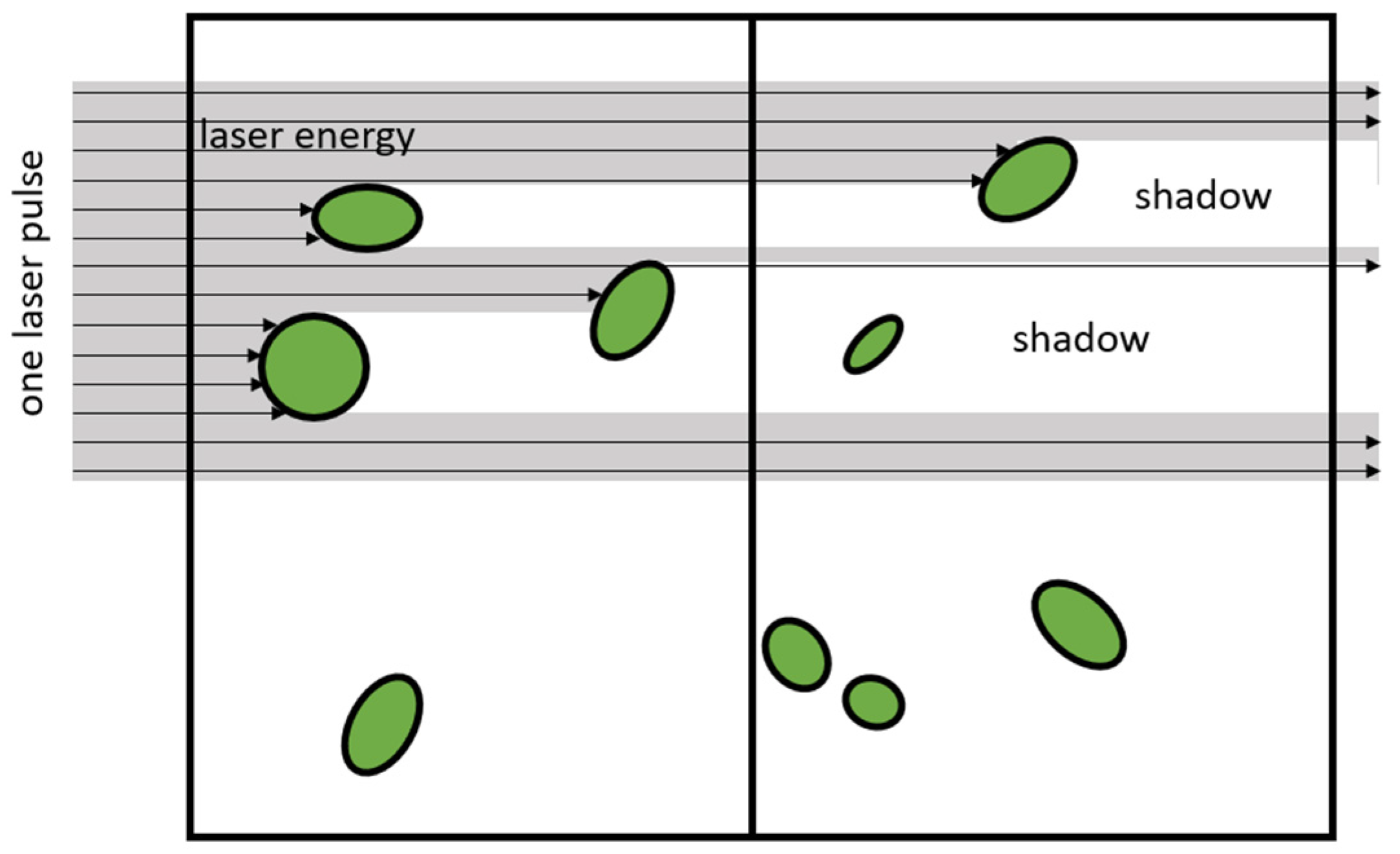
The diameter of the laser ray varies from one device to the next. It diverges slightly with distance from the scanner. For airborne laser scanners, the diameter of the laser ray is of the order of 0.3 m. In this case, most vegetation objects are smaller than the laser ray. The light is scattered on its path according to the projected area of the scattering surface. The surface is to be treated as porous. This situation is sketched in Figure 2.
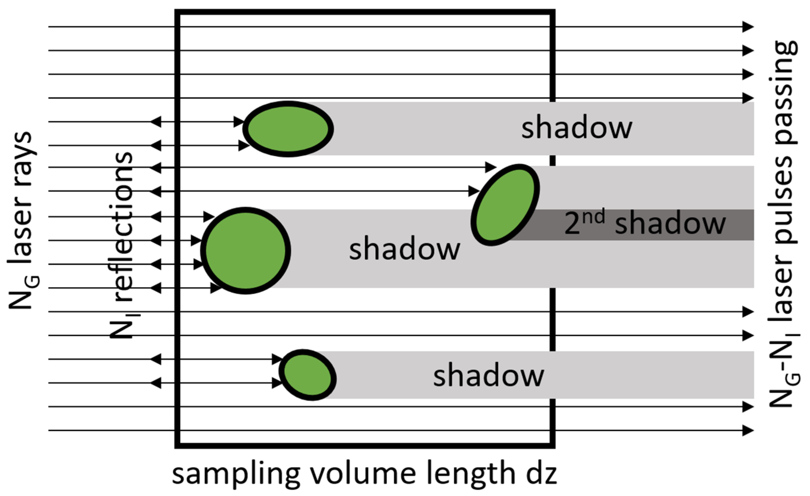
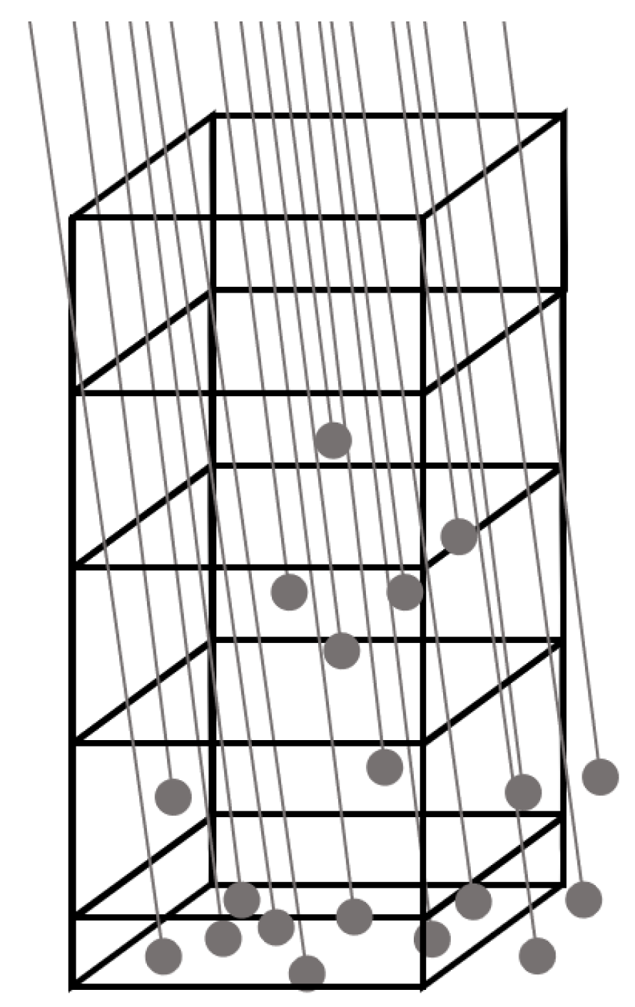
The laser beam entering the sketched volume from the left side arrives directly from the laser scanner. It hits some vegetation parts as drawn. At these surfaces, the light is scattered and part of the light returns to the scanner in the direction to the left in the sketch. The light scattered back from the vegetation parts can freely return to the scanner device without hitting any other object. Behind the vegetation parts—to the right in the sketch—is a shadow of the laser light. Any object shadowed this way cannot be detected by the laser scanner. For the hydraulic computation, the sum of the projected area of all vegetation parts in the sampling volume is needed, giving another area. This fraction can be analyzed by subdividing the laser beam into a larger number of beams with a smaller diameter, as drawn in Figure 3.
Figure 3 is a two-dimensional cross-section of a sampling volume hit by a larger number of test beams from the left side. The length of this sampling volume in the direction of the laser beam is . If the number of test rays is and is the number of reflected beams, the relation corresponds to the projection of all vegetation parts in the direction of the laser beam. If a plant part covers an area of within the sampling volume , then its relation to the sampling area cross-section is given by and describes the probability of a random laser ray to hit this surface and give a point. For a very long sampling volume, the probability to hit the surface tends to one when approaches . For a very short sampling volume with a small in the direction of the laser light, the number of vegetation parts diminishes, and thus the area . If is smaller than the diameter of the vegetation part then reflection occurs only at the real surface within this slice and the surface cutting the vegetation part is not to be accounted for. Thus, the number of reflection points in the sampling volume per approaches the value corresponding to the real vegetation density parameter we are looking for.
The shadowing (or clumping) of different vegetation parts appears only for larger lengths of sampling volumes . Therefore we keep the length small. The following law for the number of the reflected beams NI is then valid:
where is the number test rays. In the direction of the laser beam we may consider the difference between the numbers of test beams entering the sampling volume and the number leaving it. This difference is the number of hits that are reflected back along the free pathway and finally detected by the scanner. This difference reduces the number of direct rays by over one sampling volume length and can be used in Equation (11):
The integration of Equation (13) shows that even for a constant vegetation density the number of test rays decays exponentially with distance z:
This damping law is the Beer–Lambert law when the number of beams is taken as the concentration and the attenuation coefficient is one. The shadowing or clumping of vegetation parts is accounted for by this law. The number of beams decreases with distance z as in a common exponential decay function. This law gives the integral form to be used when analyzing sampling volumes of larger thickness and with larger vegetation densities to inherit the shadowing effect. It returns the homogenized vegetation density for that part. The Beer–Lambert law was described in [41].
3.2. Full Waveform Laser Processing
The standard processing of ALS data does not deliver the extensive information of the complete waveforms. Several methods [39] (1. zero crossings, 2. maximum, 3. center of gravity, 4. threshold, 5. constant fraction) exist for the processing of the backscatter signal to detect the ground surface or other objects. As shown in [39], the shift of the detected pulses to the true distance depends on the specific scatterer type. The ground level can be detected best. The detected peaks of the backscatter signal are selected and transformed into geodetic coordinates. In the examples below, the number of recorded return pulses ranged from one to four. Because of this procedure, the derivation of the cross-section for the case of a beam that has a larger diameter than the objects is not directly applicable to the three-dimensional laser scanning information. Nevertheless, the return pulses correspond to a significant level of backscattered energy. This energy corresponds to a significant cross-section of the scatterer. Therefore, they may be treated as individual reflections as in the case when the scatterer is larger than the beam diameter, depicted in Figure 3.
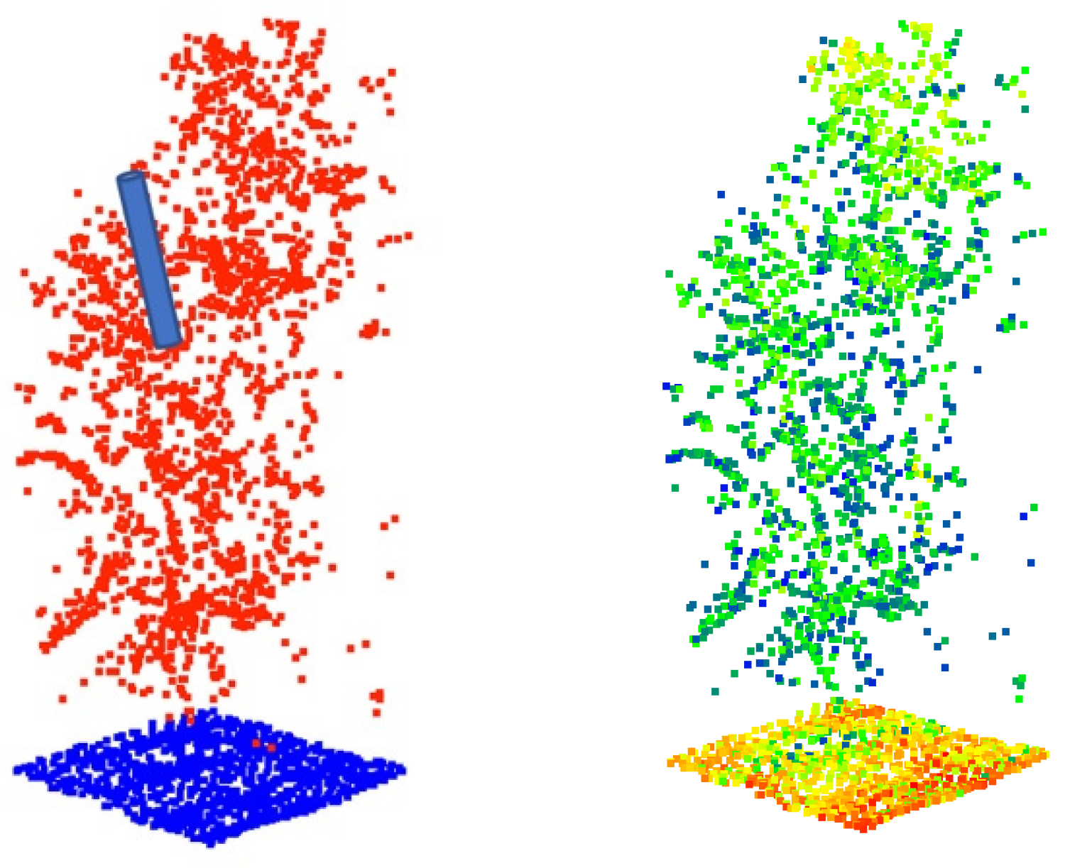
The accuracy of the ALS data is limited by the laser pulse length and the diode sampling interval. The scanner LMS-Q780 has a sampling interval of 1 ns and a pulse length of 4 ns. The laser is infrared with a 1 µm wavelength. In the air, the pulse is about 1.2 m long. The diameter depends on the distance from the instrument but amounts to about 0.3 m for common utilization. The original laser pulse may be thought of as a very long cylinder in the direction of the laser as sketched in Figure 4. In full-waveform processing, the recording of the return pulse starts when a threshold value in the return signal is exceeded. The accuracy is increased by interpolating between the samples. Targets that are less than 0.3 m apart cannot be distinguished by this technique (“dead time”).
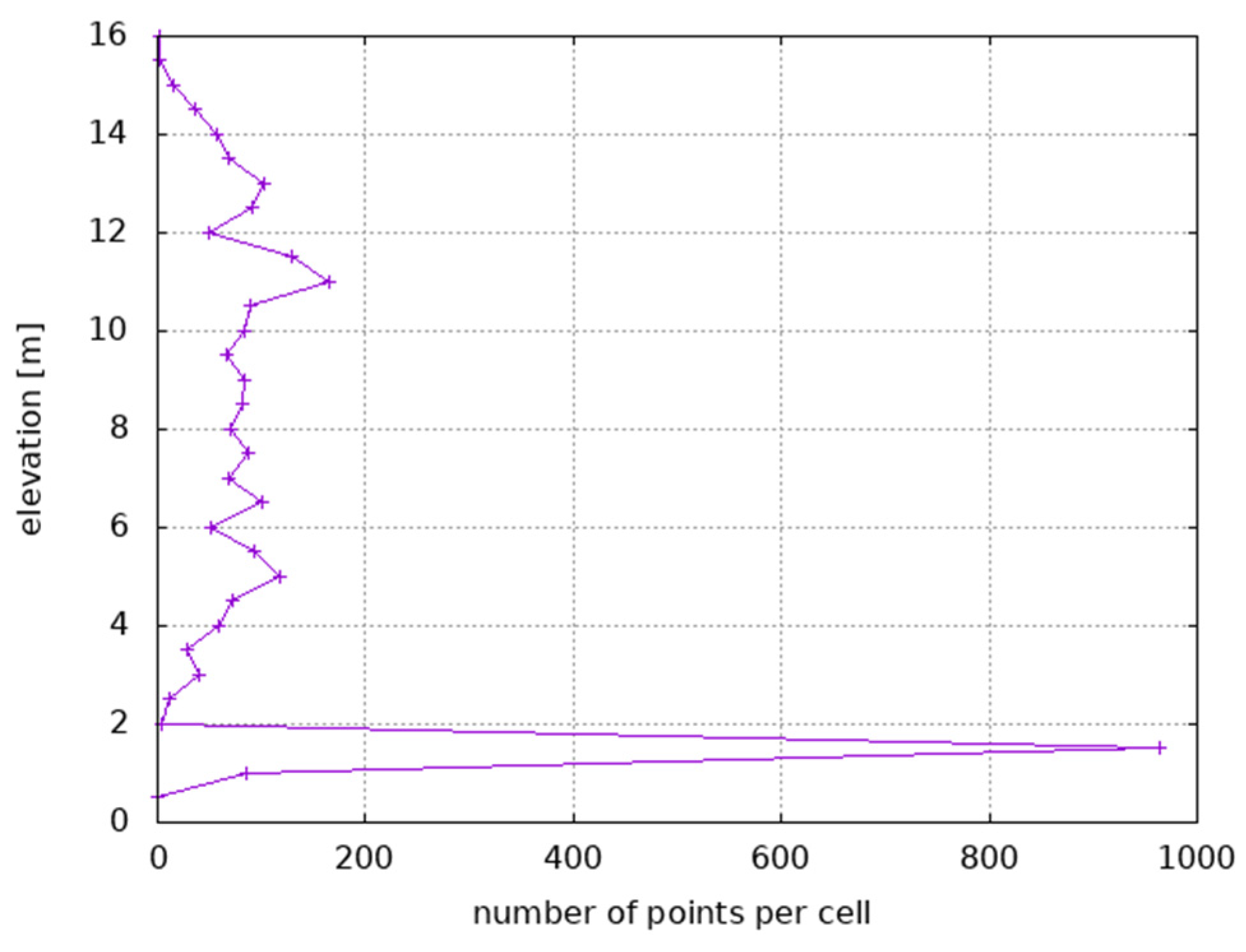
The final reflection coordinates were computed after convolution. To test the resolution of the ALS data for the small spot shown in Figure 4, the vertical profiles of the number of pulses per 0.5 m cell height are shown. Clearly, the terrain surface gives the sharpest pulse and the vegetation above is much less dense.
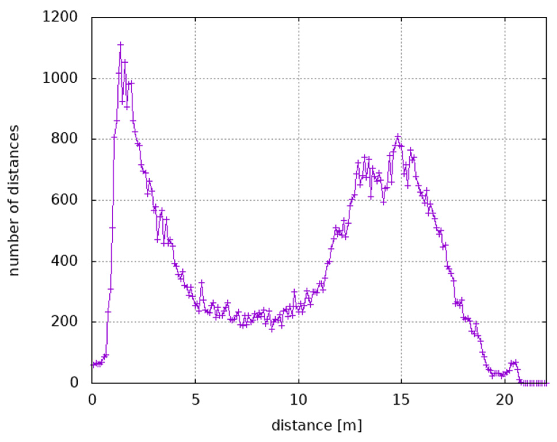
To test the separation sharpness, the distance between consecutive return pulses of each individual laser pulse was computed from the data set shown in Figure 4. Of course, not all laser pulses resulted in several reflection points. These were not considered. Figure 5 shows that the distance is not as random as should be expected, but has two clearly visible maxima and a very clear minimum for short distances. At the left side of the figure, the minimum indicates that the method cannot distinguish between objects that are less than 1 m apart. The first maximum at a bit less than 2 m indicates that in dense vegetation most of the closest reflection points are at this distance. Most frequent flooding occurs in this range close to the ground. To utilize the ALS data for flood modeling, we should connect the last pulses together. We can only estimate the ground vegetation layer by the information from one meter elevation above the ground. The second maximum in the right half of Figure 6 indicates higher vegetation that is evidently sensed well.
3.3. Description of the Proposed Procedure
The vegetation parameter is determined in a coarse three-dimensional voxel grid. The voxel size is a few meters in the horizontal and half a meter in the vertical direction. The area fraction is the area of the projection of all vegetation parts onto a surface or screen. In hydraulic computations, the flow resistance should be calculated for surfaces with normal directions oriented horizontally. ALS is sensing surfaces with vertically oriented normal directions.
The procedure proposed here relies on the following assumptions:
- The laser ray shedding is nearly parallel.
- The direction of the rays is nearly vertical downward; 20° in practice.
- The vertical projection and the horizontal projection of the vegetation area are the same.
- The number of reflection points of the laser rays divided by the number of imposed rays gives the area fraction of the vegetation inside each voxel.
The number of rays that went through each individual voxel without hitting a vegetation part is estimated by the reflexion points below that voxel, including the reflexion points at the ground surface. After the passage of each voxel, the number of test rays diminishes. The calculation procedure is as follows:
- For each voxel, the number of reflexion points Ni is counted. Additionally, a ground box or voxel of different height may be defined, where the number of reflexion points is counted as well.
- Summing up the reflexion points from the ground vertically upwards to the top gives the number of test rays that entered a voxel column Nin, i at the top:
The relevant vegetation parameter is computed using the Beer–Lambert law:
The vegetation density in voxel above ground is computed as:
The area fraction gives numbers between 0 and 1. At the ground surface, an area fraction of 1 would be computed by the last pulse data. This is depicted in Figure 7.
4. Case Study for the Kinzig Watercourse
4.1. Study Area
The Kinzig is a small watercourse north-west of Frankfurt-Main in Germany. It originates between the hilly regions of the Rhön and the Spessart and discharges into the river Main in the town Hanau. The complete length of the Kinzig is 86 km and its mean discharge at the mouth is 10 m³/s. The complete catchment area is 1058 km².
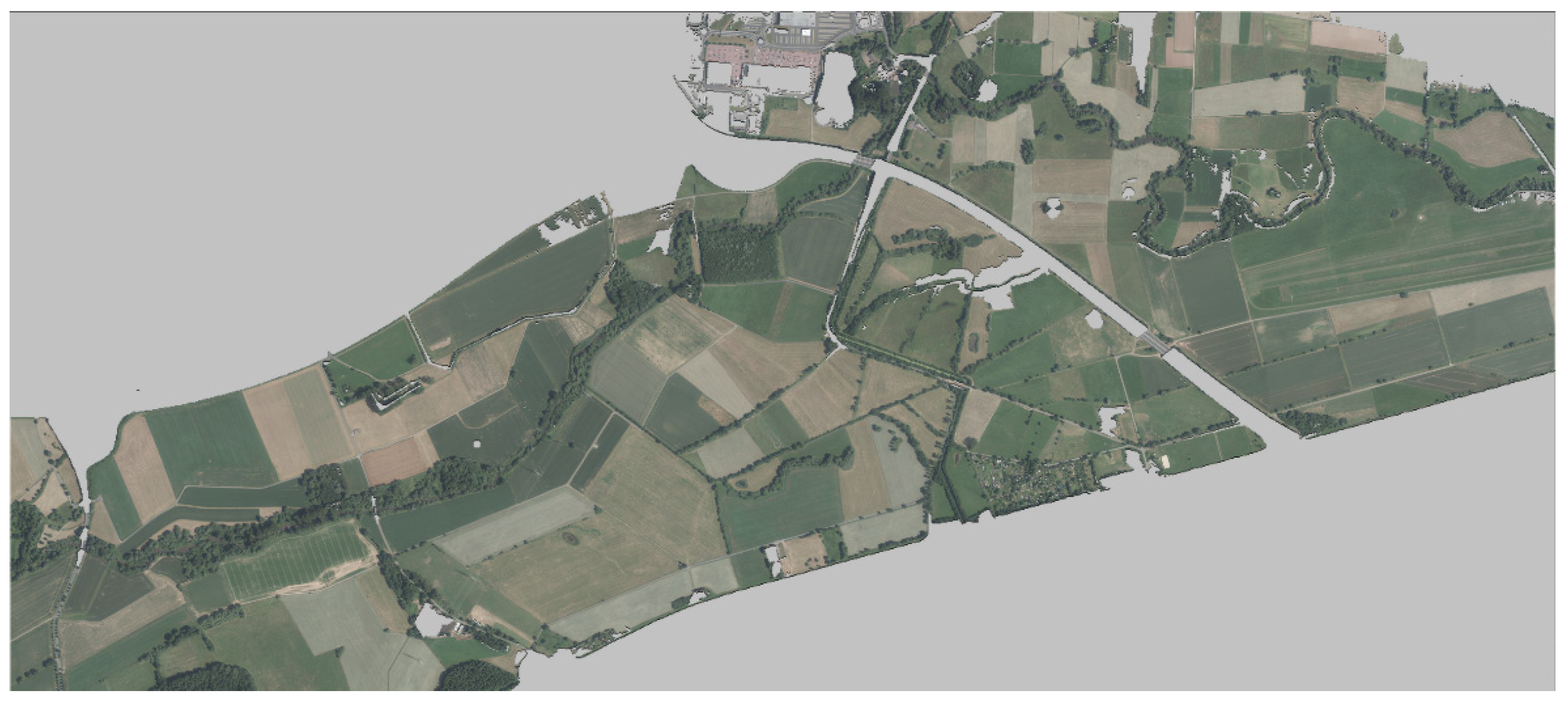
To test the method, a model of the river meadow of the Kinzig watercourse of width 3 km and length 4.8 km was set up with a one-meter resolution. This area can be seen in Figure 8. The Kinzig flows through a valley with field crops and different land use. Along the banklines, a dense canopy develops. The riparian vegetation is kept in a natural state. Deadwood is frequent in the river course.
The discharge was measured at a gauging station 200 m upstream of the model boundary. The discharge with a 100-year recurrence interval was 202 m³/s. The downstream water level was only roughly estimated and had no effect on the flow depth in the center part of the model. The water level difference was 7.1 m over the straight distance of 4.8 km, resulting in a general slope of 1.5‰. The Kinzig has a sinuosity in this reach but during a flood, the river flows in the more or less straight valley. A highway crossing the Kinzig dams the flood and concentrates the flow at only two passages. The study site was located downstream of that barrage. The ground roughness was chosen to be a constant for simplicity. The Manning–Strickler value of 40 m1/3/s was used.
In this part, profound terrain information based on ALS was set up by the state of Hessen. The actual campaign is still progressing and will be finished in 2021. The scanner is a Riegl LMS VQ780i. The laser wavelength is in the near-infrared part of the spectrum. Automatically generated 3D points as stored and available from the Hessian State Office for Land Management and Geo-Information are used in this paragraph to generate the ground level and the vegetation density with the method described above. The terrain information was derived from the last pulse data. Where no pulse was available, it was assumed that the laser beam met a water surface. Here, the ground level was derived from the interpolated bankline level and set 0.3 m deeper to account for the watercourse.
4.2. Flood Model Results
The vegetation density was derived from the complete three-dimensional ALS cloud with all return pulses for the complete domain. The vertical size of the voxels was 0.5 m and the horizontal size was one meter. At the ground level, a distance of 0.2 m was attributed to ground roughness. Therefore, the grid starts 0.2 m elevated above the ground. The densities were kept as short integer values to save memory and disk space. For the two-dimensional computation, the densities were averaged vertically from ground level to each 0.5 m voxel before the computation to obtain an averaged density for the depth-integrated computation. Depending on the water level, the densities were updated every second of model time.
To show the influence of the vegetation in this study area, two cases were considered: one with vegetation, and the other without vegetation and accounting only for the ground roughness. First the case with vegetation is shown.
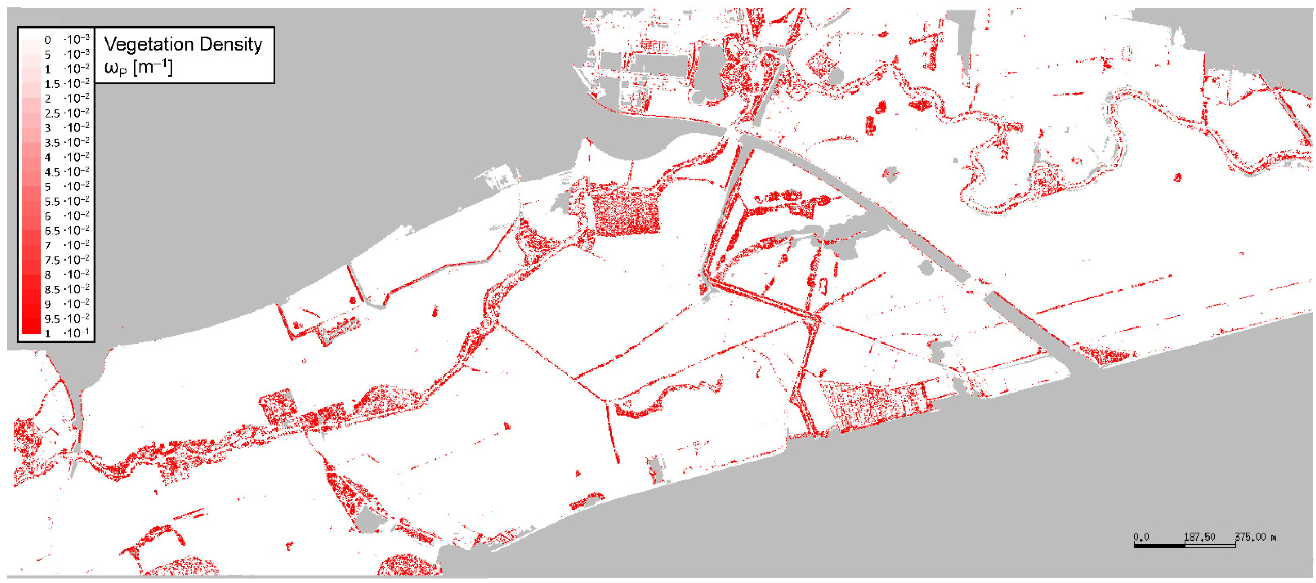
In Figure 9, the distribution of the vegetation density is plotted for the model area. The largest values, as shown by the scale in yellow, appear along the banklines of the Kinzig watercourse. These are bushes and trees, as well as deadwood in the watercourse. Most area is used for farmland and was flat during wintertime when the ALS data were derived.
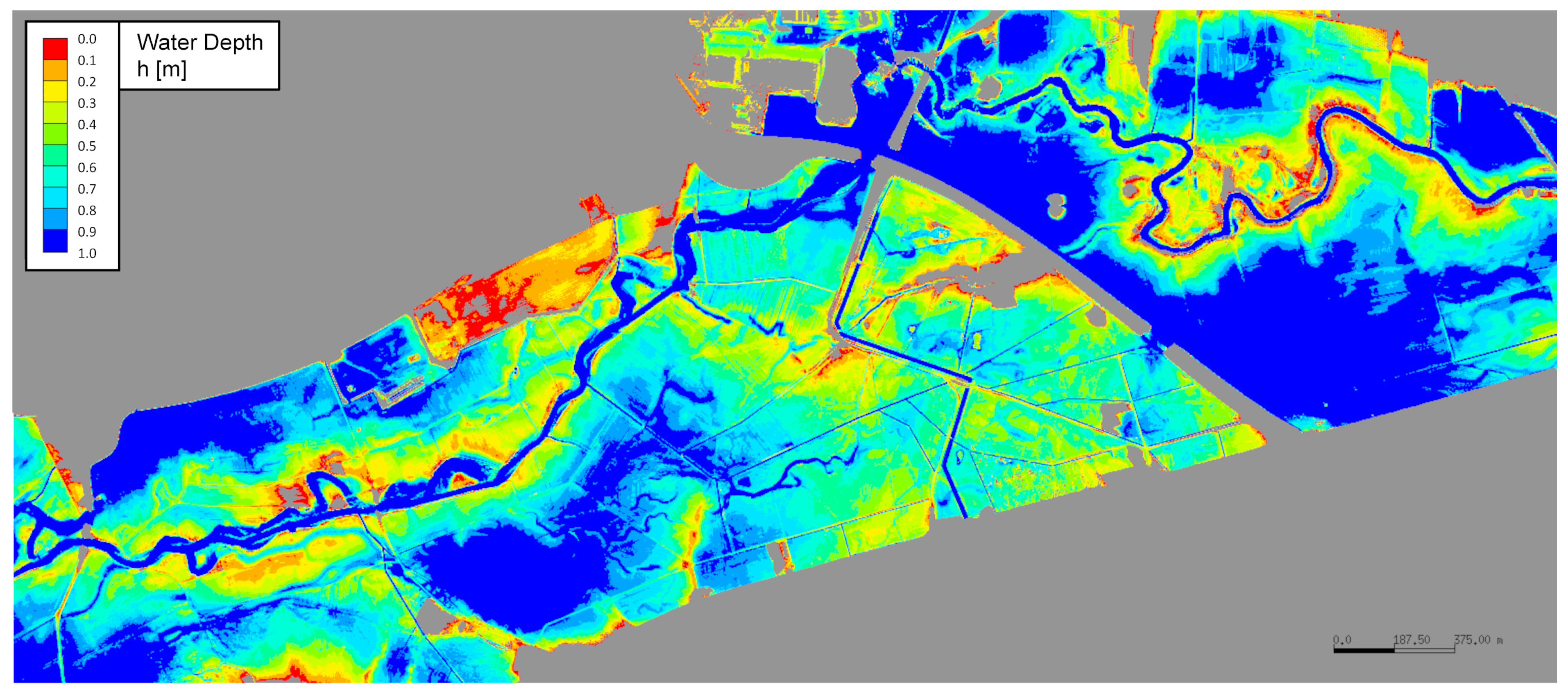
The numerical shallow water model is described in [12,42]. It was started from dry conditions and reached a steady state with stationary values after three hours of model time. The computational time step was fixed with 0.01 s. The resulting flow depth is shown in Figure 10. Clearly, the largest water depth is observed within the original watercourse Kinzig. In the upper-right part of the figure, a backwater effect is observed, induced by the highway dam, resulting in a light blue color. In the central part of the figure, water depth is about 0.5 to 1 m where a small woodland is located. The flow velocities are shown in Figure 11. They reach the maximum values under the two bridges of the highway. In most parts of the model, the velocities reach values of 0.3 to 0.4 m/s. At these velocities, the flow resistance of the bed and the vegetation is significant.
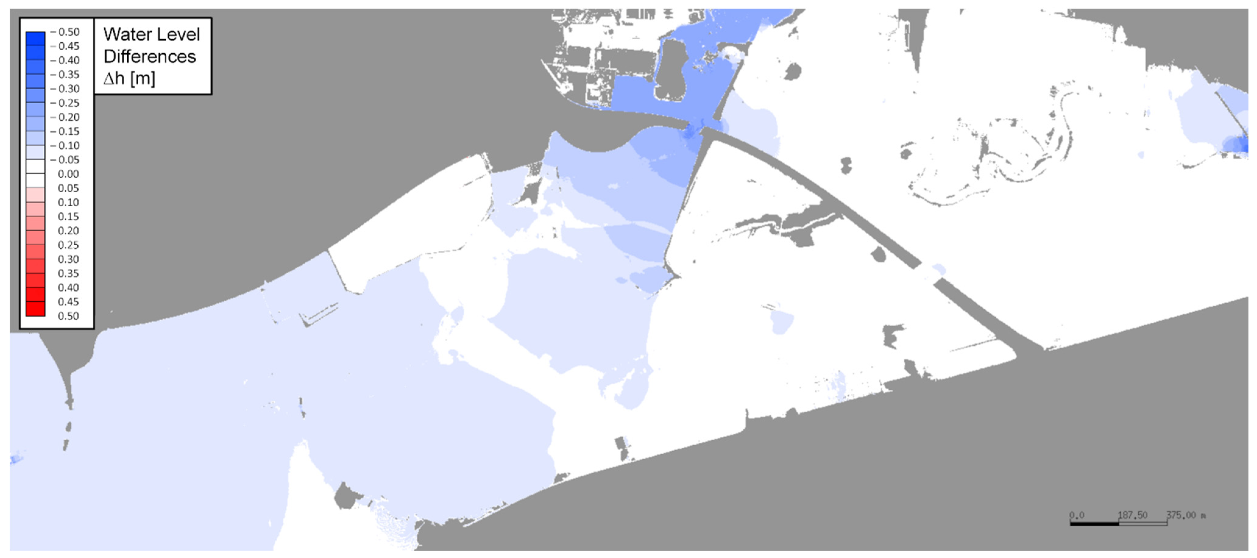
To quantify the influence of the vegetation resistance an additional model run was carried out without the vegetation resistance, and thus accounting only for the ground roughness by the Manning–Strickler value of 40 m1/3/s. As can be seen in Figure 12, the vegetation is responsible for up to 40 cm water level differences in some parts of the computational domain. Clearly, the differences are largest where the flow velocities are highest. This is around the main course of the river and in constrictions. The constriction in the upper part of the image is clearly highly influenced by vegetation, as can be seen in Figure 9. At this location, bushes grow upstream and downstream of the constriction. The second constriction in the middle of the figure is almost free of vegetation. The differences are correspondingly small; almost less than 10 cm.
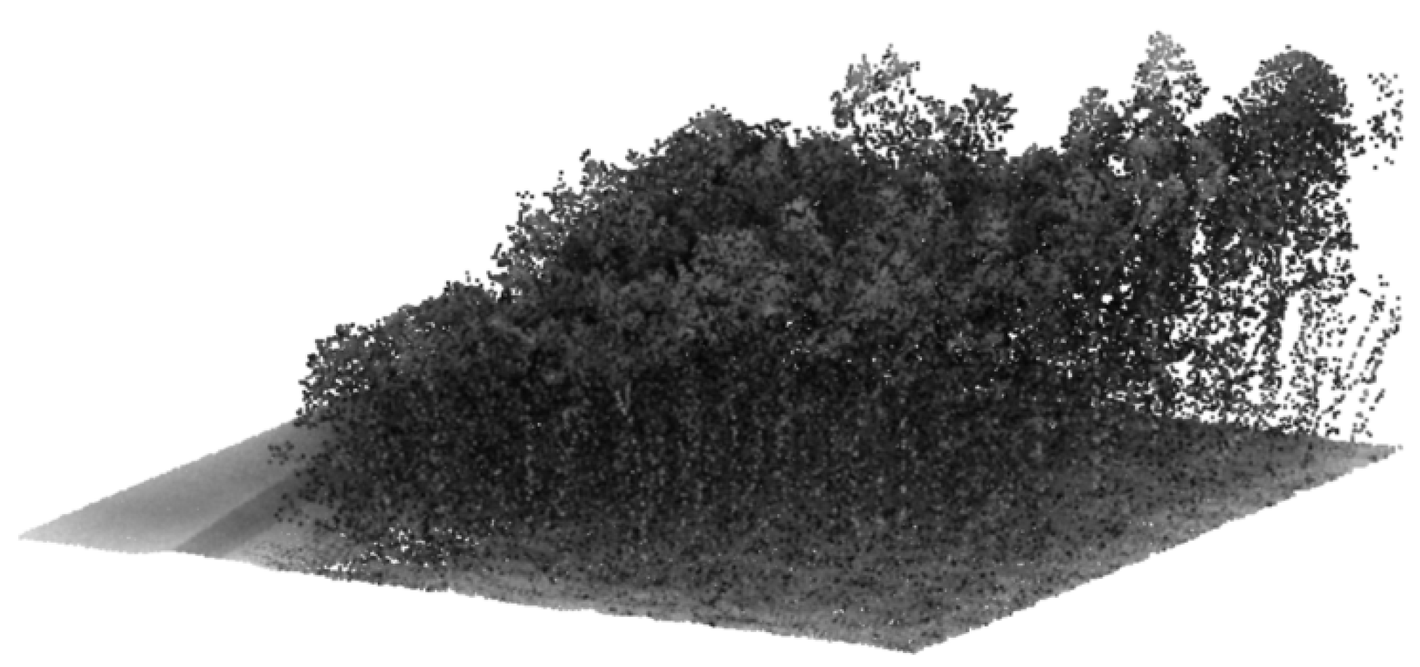
A woodland is located in the central part of the model that floods even during less severe flood events. The three-dimensional ALS data for the woodland are shown in Figure 13. The example box is shown in Figure 1 by the yellow box. It is located at the coordinates 509,760, 5,560,550 and has a size of 50 m by 50 m. In this box, 184,986 return pulses were recorded. The density is 74 points per square meter. Even individual larger trees can be identified in the dataset. Some smaller bushes are also visible near the ground surface.
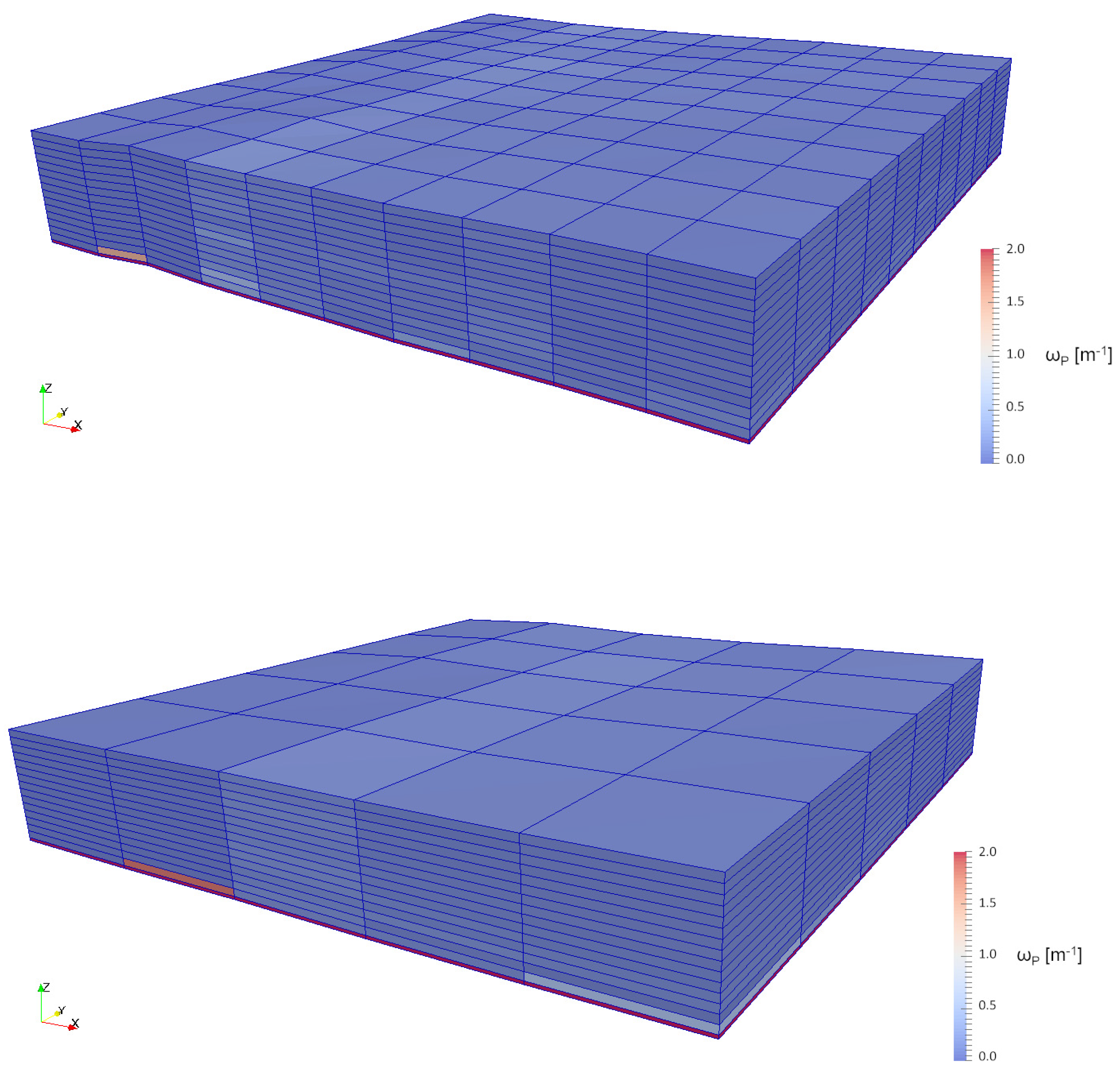
For the same area as in Figure 13, the derived vegetation density values are shown in Figure 14 for four different voxel sizes. On the right-hand side of the figures, the woodland ended, as can be seen in Figure 11. Here, the vegetation density is zero above the 0.2 m voxel for the ground zone. Clearly, the larger the voxels, the smoother the vegetation density distribution. De Almeida et al. [38] determined 5 m as the best voxel size. Here, the ALS data density is higher. The 2 m voxel size shows a good and smooth distribution of the vegetation parameter. Values for the derived vegetation density up to 0.5 m−1 can be seen in Figure 14. At several spots close to the ground, inside the volume even higher values are computed. The density compares well with a loose woodland density during wintertime.
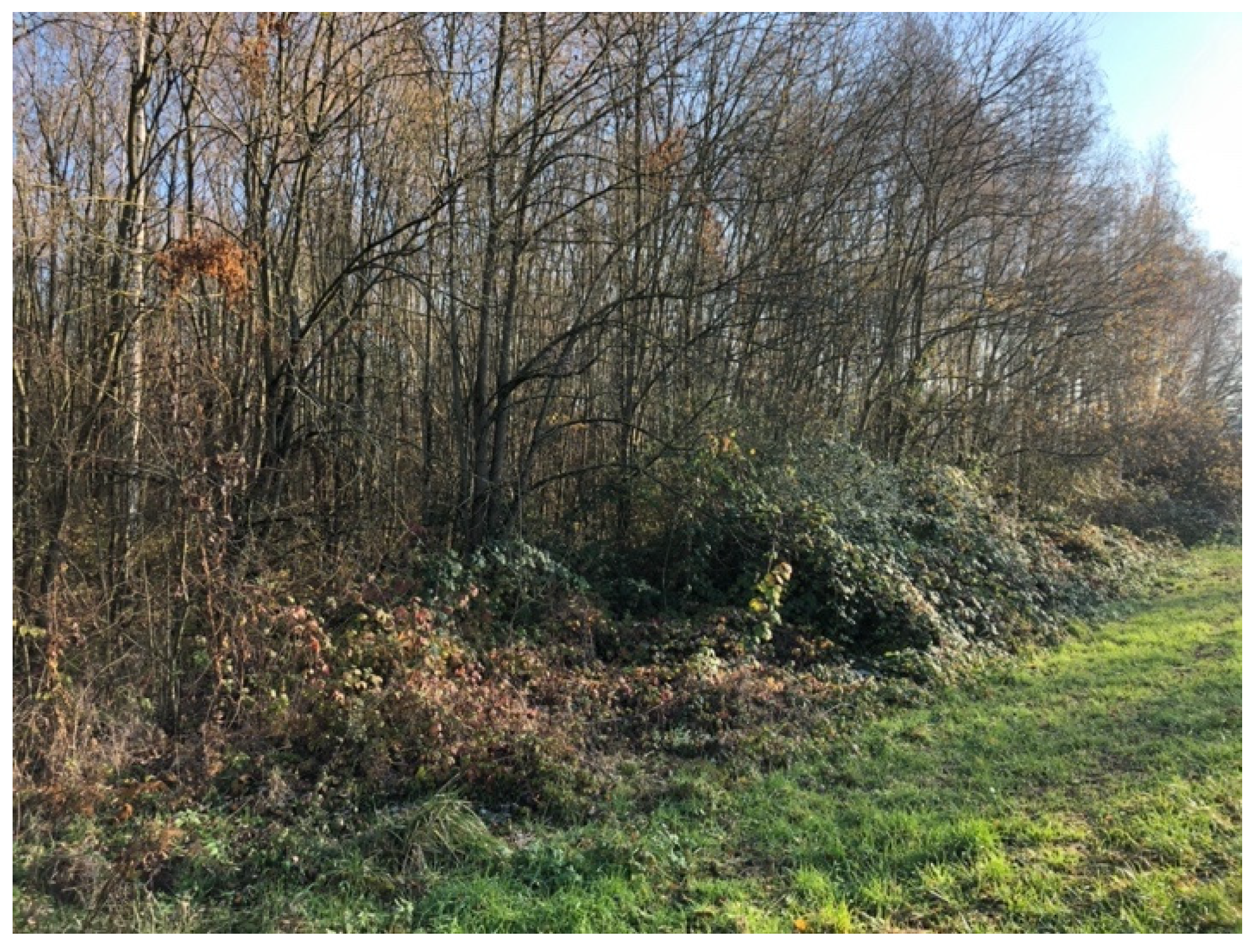
The front of the woodland is shown in Figure 15. The photograph was taken near a maintenance road, in the direction opposite to the view direction in Figure 13 and Figure 14. The density of the trees is not very high. During wintertime, it is possible to see objects up to a distance of more than 50 m. This corresponds roughly to a vegetation density of 0.02 m−1. It can also be observed that at the edge of the woodland the branches of the trees grow to the side, where they obtain more sunlight. Some bushes and brambles also grow in this part. The brambles were dense enough to blot out the laser pulse completely. Here, the model ground level shows a little bump.
5. Conclusions
Flood water levels are highly influenced by the presence of vegetation in the flow. The incorporation of the hydraulic vegetation resistance in the flood computations is straightforward using the vegetation density as given in Equation (4). In the field this geometric parameter can only be estimated from maps or from local measurements. The most recent airborne laser scanning (ALS) campaigns deliver high-quality three-dimensional data sets with a point density of more than 10 points per square meter. The data density reached a level that made the data suitable for the estimation of vegetation flow resistance. A procedure to derive the corresponding vegetation density and flow resistance coefficients is described in this paper.
The data available are not the full waveform data. Nevertheless, the data volume is very high and can amount to over 70 points per square meter, as in the case study. This amount of information is sufficient to estimate the vegetation density at different levels above the ground. A horizontal resolution of one meter is possible. The laser scanner data acquisition technique sets limits regarding the differentiation of individual plants. The relation between the diameters of the laser beam and the vegetation parts is considered for ALS and TLS data and the computation procedure described in Section 3.3. This procedure is independent from human interference and thus can be seen as an objective grounds for the estimation of the vegetation-induced flow resistance.
The proposed procedure was applied in a case study for the river Kinzig. The vegetation densities and the corresponding flow resistance coefficients were evaluated. The values compare well with those given in the literature. The resistance approach was implemented and used in a two-dimensional flow model. The computed water level differences due to vegetation are shown by a comparison of two model computations.
The detailed and complete new ALS data allow for very detailed flow computations, as shown in Figure 11. The very heterogeneous vegetation close to a river is well sensed and reproduced in the flood model by the method described here.
Even though the obtained values compare well with the standard values tabulated for use in practical applications, it is desirable to confirm the values and the method by extensive field measurements. Field data for the actual hydraulic resistance of specific stands and types of vegetation are hard to obtain and still scarce.
Funding
This research is closely related to a project supported by the German Federal Ministry for Economic Affairs and Energy in the ZIM initiative for “Development of new techniques in computer modeling for flood prevention”.
Informed Consent Statement
Not applicable.
Data Availability Statement
Restrictions apply to the availability of ALS data. Data was obtained from Hessian State Office for Land Management and Geo-Information and are available only with the permission of the Hessian State Office.
Acknowledgments
The author acknowledges the Hessian State Office for Land Management and Geo-Information for providing the laser scan data and the arial image used in this article.
Conflicts of Interest
The author declares no conflict of interest. The funders had no role in the design of the study; in the collection, analyses, or interpretation of data; in the writing of the manuscript; or in the decision to publish the results.
References
- Arcement, G.J.; Schneider, V.R. Guide for Selecting Manning’s Roughness Coefficients for Natural Channels and Flood Plains; U.S. Geological Survey Water-Supply Paper 2339; U.S. Government Publishing Office: Washington, DC, USA, 1989.
- Järvelä, J. Determination of flow resistance caused by non-submerged woody vegetation. Int. J. River Basin Manag. 2004, 2, 61–70. [Google Scholar] [CrossRef]
- Straatsma, M.W.; Baptist, M.J. Floodplain roughness parameterization using airborne laser scanning and spectral remote sensing. Remote Sens. Environ. 2008, 112, 1062–1080. [Google Scholar] [CrossRef]
- Forzieri, G.; Castelli, F.; Preti, F. Advances in remote sensing of hydraulic roughness. Int. J. Remote Sens. 2012, 33, 630–654. [Google Scholar] [CrossRef]
- Luo, S.; Wang, C.; Pan, F.; Xi, X.; Li, G.; Nie, S.; Xia, S. Estimation of wetland vegetation height and leaf area index using airborne laser scanning data. Ecol. Indic. 2015, 48, 550–559. [Google Scholar] [CrossRef]
- Wang, C.; Zheng, S.; Wang, P.; Hou, J. Interactions between vegetation, water flow and sediment transport: A review. J. Hydrodyn. Ser. B 2015, 27, 24–37. [Google Scholar] [CrossRef]
- DFG-Forschungsbericht, Hydraulische Probleme beim Naturnahen Gewässerausbau; VCH-Verlagsgesellschaft: Weinheim, Germany, 1987.
- Lindner, K. Der Strömungswiderstand von Pflanzenbeständen, Mitteilung des Leichtweiss-Institut für Wasserbau, Heft 75; Leichtweiss-Inst. für Wasserbau: Braunschweig, Germany, 1982. [Google Scholar]
- DVWK Heft 220, Hydraulische Berechnung von Fließgewässern, Merkblatt zur Wasserwirtschaft; Deutsche Vereinigung für Wasserwirtschaft, Abwasser und Abfall: Hamburg/Berlin, Germany, 1991.
- Bretschneider, H.; Schulz, A. Anwendung von Fließformeln bei Naturnahem Gewässerausbau, Schriftenreihe des DVWK, Heft 72; Verlag Paul Parey: Hamburg, Germany, 1985. [Google Scholar]
- BWK. Hydraulische Berechnung von Naturnahen Fließgewässern—Teil 2; Bund der Ingenieure für Wasserwirtschaft, Abfallwirtschaft und Kulturbau (BWK e.V.): Pfullingen, Germany, 2000. [Google Scholar]
- Mewis, P. Numerische Berechnungen zum Einfluss Verschiedener Bewuchsstadien auf das Fließgeschehen, Darmstädter Wasserbauliches Kolloquium 1996. In Mitteilungen des Institutes für Wasserbau; Heft 98; TU-Darmstadt: Darmstadt, Germany, 1997; pp. 237–249. [Google Scholar]
- Petryk, S.; Bosmajian, G. Analysis of flow through vegetation. J. Hydr. Div. ASCE 1975, 101, 871–884. [Google Scholar] [CrossRef]
- Zahidi, I.; Yusuf, B.; Cope, M.; Mohamed, T.A.; Shafri, H.Z.M. Effects of depth-varying vegetation roughness in two-dimensional hydrodynamic modelling. Int. J. River Basin Manag. 2018, 16. [Google Scholar] [CrossRef]
- Jalonen, J.; Järvelä, J.; Aberle, J. Leaf Area Index as Vegetation Density Measure for Hydraulic Analyses. J. Hydraul. Eng. 2013, 139. [Google Scholar] [CrossRef]
- Luhar, M.; Nepf, H.M. Flow-induced reconfiguration of buoyant and flexible aquatic vegetation. Limnol. Oceanogr. 2011, 56, 2003–2017. [Google Scholar] [CrossRef] [Green Version]
- Schoneboom, T. Widerstand Flexibler Vegetation und Sohlenwiderstand in durchströmten Bewuchsfeldern. Ph.D. Dissertation, TU Braunschweig, Braunschweig, Germany, 2011. [Google Scholar]
- Stephan, U.; Gutknecht, D. Hydraulic resistance of submerged flexible vegetation. J. Hydrol. 2002, 269, 27–43. [Google Scholar] [CrossRef]
- Stephan, U. Zum Fließwiderstandsverhalten Flexibler Vegetation. Wiener Mitteilungen des Instituts für Hydraulik, Gewässerkunde und Wasserwirtschaft; Band 180; Technische Universität Wien: Wien, Germany, 2002. [Google Scholar]
- Västilä, K.; Järvelä, J. Modeling the flow resistance of woody vegetation using physically based properties of the foliage and stem. Water Resour. Res. 2014, 50, 229–245. [Google Scholar] [CrossRef]
- Schneider, S. Widerstandsverhalten von holzigen Auenpflanzen—Konzept zur Etablierung von Weichholzauen an Fließgewässern. Ph.D. Dissertation, Karlsruher Institut für Technologie (KIT), Karlsruhe, Germany, 2010. [Google Scholar]
- Wunder, S. Zum Fließverhalten um strauchartige Weidengewächse und dessen Auswirkungen auf den Strömungswiderstand. Ph.D. Dissertation, Universität Karlsruhe KIT, Karlsruhe, Germany, 2014. [Google Scholar]
- Hartlieb, A. Modellversuche zur Rauheit durch- bzw. überströmter Maisfelder, Wasserwirtschaft, Nr. 3/2006; Wasserwirtschaft: Wiesbaden, Germany, 2006; pp. 38–41. [Google Scholar]
- Habersack, H. Zusammenstellung von kst-Rauheitsbeiwerten, BOKU Wien. Available online: http://iwhw.boku.ac.at/LVA816332/Flie%E1widerstand_Einheit_5.pdf (accessed on 12 March 2018).
- Antonarakis, A.S.; Richards, K.S.; Brasington, J.; Muller, E. Determining leaf area index and leafy tree roughness using terrestrial laser scanning. Water Resour. Res. 2010, 46, W06510. [Google Scholar] [CrossRef] [Green Version]
- Wohlfahrt, G.; Sapinsky, S.; Tappeiner, U.; Cernusca, A. Estimation of plant area index of grasslands from measurements of canopy radiation profiles. Agric. For. Meteorol. 2001, 109, 1–12. [Google Scholar] [CrossRef]
- Oplatka, M. Stabilität von Weidenverbauungen an Flussufern; Heft 156; Mitteilungen der Versuchsanstalt für Hydrologie und Glaziologie der Eidgenössischen Technischen Hochschule: Zürich, Switzerland, 1998. [Google Scholar]
- Toda, M.; Richardson, A.D. Estimation of plant area index and phenological transition dates from digital repeat photography and radiometric approaches in a hardwood forest in the Northeastern United States. Agric. For. Meteorol. 2018, 249, 457–466. [Google Scholar] [CrossRef]
- Ogunbadewa, E.Y. Tracking seasonal changes in vegetation phenology with a SunScan canopy analyzer in northwestern England. For. Sci. Technol. 2012, 8, 161–172. [Google Scholar] [CrossRef]
- Peduzzi, A.; Wynne, R.H.; Fox, T.R.; Nelson, R.F.; Thomas, V.A. Estimating leaf area index in intensively managed pine plantations using airborne laser scanner data. For. Ecol. Manag. 2012, 270, 54–65. [Google Scholar] [CrossRef] [Green Version]
- Parker, G.; Harding, D.J.; Berger, M.L. A portable LIDAR system for rapid determination of forest canopy structure. J. Appl. Ecol. 2004, 41, 755–767. [Google Scholar] [CrossRef]
- Hosoi, F.; Omasa, K. Voxel-Based 3-D Modeling of Individual Trees for Estimating Leaf Area Density Using High-Resolution Portable Scanning Lidar. IEEE Trans. Geosci. Remote Sens. 2006, 44, 12. [Google Scholar] [CrossRef]
- Jalonen, J.; Järvelä, J.; Virtanen, J.-P.; Vaaja, M.; Kurkela, M.; Hyyppä, H. Determining Characteristic Vegetation Areas by Terrestrial Laser Scanning for Floodplain Flow Modeling. Water 2015, 7, 420–437. [Google Scholar] [CrossRef] [Green Version]
- Blair, J.B.; Rabine, D.L.; Hofton, M.A. The Laser Vegetation Imaging Sensor: A medium-altitude, digitisation-only, airborne laser altimeter for mapping vegetation and topography. ISPRS J. Photogramm. Remote Sens. 1999, 54, 115–122. [Google Scholar] [CrossRef]
- Lovell, J.L.; Jupp, D.L.B.; Culvenor, D.S.; Coops, N.C. Using airborne and ground-based ranging lidar to measure canopy structure in Australian forests. Can. J. Remote Sens. 2003, 29, 607–622. [Google Scholar] [CrossRef]
- Fewtrell, T.J.; Duncan, A.; Sampson, C.C.; Neal, J.C.; Bates, P.D. Benchmarking urban flood models of varying complexity and scale using high resolution terrestrial LiDAR data. Phys. Chem. Earth 2011, 36, 281–291. [Google Scholar] [CrossRef]
- Wessels, M.; Brückner, N.; Gaide, S.; Wintersteller, P. Tiefenschärfe—Die Hochauflösende Vermessung des Bodensees; Wasserwirtschaft: Wiesbaden, Germany, 2017; Volume 4. [Google Scholar]
- de Almeida, D.R.A.; Stark, S.C.; Shao, G.; Schietti, J.; Nelson, B.W.; Silva, C.A.; Gorgens, E.B.; Valbuena, R.; de Almeida Papa, D.; Brancalion, P.H.S. Optimizing the Remote Detection of Tropical Rainforest Structure with Airborne Lidar: Leaf Area Profile Sensitivity to Pulse Density and Spatial Sampling. Remote Sens. 2019, 11, 92. [Google Scholar] [CrossRef] [Green Version]
- Wagner, W.; Ullrich, A.; Melzer, T.; Briese, C.; Kraus, K. From Single-Pulse to Full-Waveform Airborne Laser Scanners: Potential and Practical Challenges. 2004. Available online: https://publik.tuwien.ac.at/files/PubDat_119591.pdf (accessed on 1 July 2021).
- Wagner, W.; Ullrich, A.; Briese, C. Der Laserstrahl und Seine Interaktion mit der Erdoberfläche. 2004. Available online: https://publik.tuwien.ac.at/files/PubDat_119558.pdf (accessed on 1 July 2021).
- MacArthur, R.H.; Horn, H.S. Foliage profile by vertical measurements. Ecology 1969, 50, 802–804. [Google Scholar] [CrossRef] [Green Version]
- Mewis, P. Sparse element for shallow water wave equations on triangle meshes. Int. J. Numer. Methods Fluids 2013, 72, 864–882. [Google Scholar] [CrossRef]
Figure 1.
Perspective view of 3D laser scan data for the Kinzig floodplain with farming land, created with Cloud Compare.
Figure 1.
Perspective view of 3D laser scan data for the Kinzig floodplain with farming land, created with Cloud Compare.

Figure 2.
Sketch of a laser beam in grey hitting two sampling volumes (boxes) from the left side. The vegetation parts are drawn in green color. They are of smaller diameter than the beam.
Figure 2.
Sketch of a laser beam in grey hitting two sampling volumes (boxes) from the left side. The vegetation parts are drawn in green color. They are of smaller diameter than the beam.

Figure 3.
Sketch of a single sampling volume completely covered by many test beams approaching from the left side and hitting some vegetation parts, drawn in green.
Figure 3.
Sketch of a single sampling volume completely covered by many test beams approaching from the left side and hitting some vegetation parts, drawn in green.

Figure 4.
Sketch of a laser pulse in the canopy investigated in the example. In the left figure the return pulses are colored by classification into ground (blue) and vegetation (red), and in the right figure by intensity. All together 2974 return pulses were available on the square with a side length of five meter.

Figure 5.
Vertical profile of return pulses in sample area shown in Figure 4 of size 5 m by 5 m.
Figure 5.
Vertical profile of return pulses in sample area shown in Figure 4 of size 5 m by 5 m.

Figure 6.
Statistics of distances between two consecutive return pulses of each laser pulse for the sample area shown in Figure 4.
Figure 6.
Statistics of distances between two consecutive return pulses of each laser pulse for the sample area shown in Figure 4.

Figure 7.
Schematic of calculation of the area fraction of vegetation by the test rays and the reflexion points.
Figure 7.
Schematic of calculation of the area fraction of vegetation by the test rays and the reflexion points.

Figure 8.
Image of the model area of the Kinzig floodplain. The dam that divides the image in the right side is a highway connection. The Kinzig flows from right to left in the figure. Land use is mostly farming. Higher vegetation occurs along the river course.
Figure 8.
Image of the model area of the Kinzig floodplain. The dam that divides the image in the right side is a highway connection. The Kinzig flows from right to left in the figure. Land use is mostly farming. Higher vegetation occurs along the river course.

Figure 9.
Vegetation density parameter from 0.005 to 0.1 m−1 in the model area.

Figure 10.
Flow depth for the stationary state. At some locations the flow depth of one meter is exceeded. Grey indicates dry areas.
Figure 10.
Flow depth for the stationary state. At some locations the flow depth of one meter is exceeded. Grey indicates dry areas.

Figure 11.
Flow velocities for the stationary state. Grey indicates dry areas.

Figure 12.
Flow depth differences between a calculation with and without vegetation resistance. Bed resistance is accounted for in both cases. Grey indicates dry areas.
Figure 12.
Flow depth differences between a calculation with and without vegetation resistance. Bed resistance is accounted for in both cases. Grey indicates dry areas.

Figure 13.
Return pulse intensities for a young forest shown in greyscale for the sample area.

Figure 14.
Vegetation parameter for a young forest close to the river Kinzig derived from ALS data with three different resolutions. Grids are 1, 2, 5 and 10 m. The vertical grid is terrain fitted, and the complete block is 8 m high, which is less than the tree height.
Figure 14.
Vegetation parameter for a young forest close to the river Kinzig derived from ALS data with three different resolutions. Grids are 1, 2, 5 and 10 m. The vertical grid is terrain fitted, and the complete block is 8 m high, which is less than the tree height.


Table 1.
Value ranges of the vegetation parameter when recomputed to skin friction parameters for two different flow depths.
Table 1.
Value ranges of the vegetation parameter when recomputed to skin friction parameters for two different flow depths.
| [m−1] | [–] | Flow velocity [m/s] for slope S = 1.5‰ | [–] | ||
| h = 1 m | h = 0.5 m | ||||
| 0.01 | 0.048 | 40.4 | 1.56 | 0.024 | 80.8 |
| 0.03 | 0.144 | 23.3 | 0.90 | 0.072 | 46.7 |
| 0.1 | 0.48 | 12.8 | 0.49 | 0.24 | 25.6 |
| 1 | 4.8 | 4.0 | 0.16 | 2.4 | 8.1 |
Publisher’s Note: MDPI stays neutral with regard to jurisdictional claims in published maps and institutional affiliations. |
© 2021 by the author. Licensee MDPI, Basel, Switzerland. This article is an open access article distributed under the terms and conditions of the Creative Commons Attribution (CC BY) license (https://creativecommons.org/licenses/by/4.0/).
Share and Cite
MDPI and ACS Style
Mewis, P. Estimation of Vegetation-Induced Flow Resistance for Hydraulic Computations Using Airborne Laser Scanning Data. Water 2021, 13, 1864. https://doi.org/10.3390/w13131864
AMA Style
Mewis P. Estimation of Vegetation-Induced Flow Resistance for Hydraulic Computations Using Airborne Laser Scanning Data. Water. 2021; 13(13):1864. https://doi.org/10.3390/w13131864
Chicago/Turabian StyleMewis, Peter. 2021. "Estimation of Vegetation-Induced Flow Resistance for Hydraulic Computations Using Airborne Laser Scanning Data" Water 13, no. 13: 1864. https://doi.org/10.3390/w13131864
Note that from the first issue of 2016, this journal uses article numbers instead of page numbers. See further details here.