
Yield Stress Model for Natural Debris Flows in Presence of Fine and Coarse–Grained Sediments


Department of Engineering, University of Ferrara, V. Saragat, 1, 44122 Ferrara, Italy
Water 2021, 13(13), 1865; https://doi.org/10.3390/w13131865
Submission received: 2 June 2021
/
Revised: 29 June 2021
/
Accepted: 29 June 2021
/
Published: 4 July 2021
Abstract
:When dealing with natural geo–hazards, it is important to understand the influence of sediment sorting on debris flows. The presence of coarse fraction is one of the aspects which affects the rheological behaviour of natural viscous granular fluid mixtures. In this paper, experiments on reconstituted debris flow mixtures with different coarse–to–fine sediment ratios are considered. Such mixtures behave just as non–Newtonian yield stress fluids and their rheological behaviour is largely affected by the presence of coarse fraction. Experimental results demonstrate that yield stress is very sensitive not only to bulk sediment concentration but also to coarse sediment fraction. A novel yield stress model is presented. It accounts for an empirical grading function depending on the coarse–to–fine grain content. The yield stress model performed satisfactorily in comparison with the experiments, showing that it is almost independent of the coarse–to–fine grain fraction in case of dominant coarse sediment content.
1. Introduction
Viscous debris flows are a very complex and important geomechanical process in subaerial and subaqueous environments. Hyperconcentrated sediments are treated in the same way as yielding non–Newtonian fluids when transported, and the rheological behaviour of such sediments has been widely tested using a variety of different experimental equipment including standard rheometric systems and even unusually large rheometers. Nonetheless, their rheological characteristics are still largely ununderstood, since they involve many factors such as soil type, sediment size distribution, grain concentration, and even other physical and chemical properties (e.g., salinity, pH, mineralogy) which are particularly relevant when very fine sediments are present. In the specific case of natural sediment, even grain shape plays a significant role [1]. With regard to the flow–like behaviour of slurries, the rate of shear deformation systematically increases as shear stress increases, but the relationships between the two differs according to sediment concentration, showing either dilatant or pseudoplastic material behaviour [2].
The travel distance of debris flow is important in hazard mapping and can be predicted based on the process of halting the slurry. The latter is controlled by the shearing material and by the circumstances under which the material ceases to move (dynamic yield stress), leading to a different condition from the one under which the material started moving (static yield stress). This mechanism has been investigated over the past decades by several authors using both conventional and non–conventional experimental apparatus [3,4,5,6]. Mostly, previous studies have concerned the effect of fine fraction and bulk sediment concentration. However, so far the role of sediment grain size distribution has been poorly investigated, partly due to the difficulties inherent in experimental apparatus and procedures.
Several authors have focused on the yielding characteristic of noncolloidal suspensions [7,8] and dense granular fluid mixtures [9,10,11,12,13]. In particular, Ancey and Jorrot [10] studied the effects of the solid concentration of unimodal and bimodal suspensions of glass beads and quartz sand in a water–kaolin dispersion on the yield stress. They found evidence that the yield stress of a coarse particle suspension within the colloidal dispersions is strongly dependent on the solid concentration of the coarse fraction.
Experimental work by Yu et al. [14] stressed the influence of clay minerals on the yield stress of debris flows, and later Yu et al. [15] carried out experiments involving mixtures of clay, and fine and coarse sand, demonstrating the influence of single clay and mixed clay mixture on the threshold stress value. Pantet et al. [16] studied the effect of coarse particle concentration on the yield stress of silty sand and muddy sand mixtures and found that the yield stress could be moderately or significantly altered by the content of coarser particles. Other authors have considered the flow–like behaviour of fine–grained slurries and demonstrated that plastic viscosity is very sensitive to the ratio between clay–silt and clay–sand fraction (e.g., [17]). Jeong et al. [18] focused on the role of soil texture, and proposed a schematic view of rheological behaviour, depending on grain size, showing a remarkable difference in rheological behaviour from fine–grained to coarse–grained slurry [19].
Coussot and Piau [20] carried out experiments on debris flow mixtures and found that coarser sediment fraction has a relevant effect on yield stress. Banfill [21] stressed the influence of fine material in sand on the rheology of fresh mortar, concluding that yield stress increases as the fine sand fraction rises. Ancey and Jorrot [10] showed that for poorly sorted materials, the rate of yield variation as a function of bulk sediment concentration very much depends on sediment characteristics and on the relative content of coarse–to–fine grains. Yu et al. [15] reported a selection of works by Chinese authors [22,23,24] who investigated the role of sediment grading on the yield stress of reconstituted debris flows, showing that the yield increased with a decreasing grain diameter, an increase in sediment concentration, and (corresponding to large particle concentration) with an increasing uniformity of particle size distribution. In their work, Yu et al. [15] suggested considering grain size distribution, particle shape, and type of material of the particles (in addition to sediment concentration) as the main aspects affecting yield stress value. Jan et al. [25] tested fine sediment slurries mixed with coarse sand at different concentrations, and showed qualitatively that the presence of coarse grains reduces the yield stress of the mixture, concluding that the rheology of the sediment slurry could vary widely depending on the particle size present in the slurry.
The previous scrutiny shows that most of the reported rheological properties of debris flows have been restricted to fine–graded mixtures, which provide the interstitial fluid matrix of viscous debris flow. However, the transition from fine–grained to coarse–grained soils is of paramount importance for the rheology, largely due to the presence of poorly sorted grains in natural slurries.
In a previous work, Pellegrino and Schippa [13] tested the effect of granular concentration and sediment grading on the rheological properties of reconstituted debris flows. In particular, for fine–grained mixtures, the Herschel–Bulkley generalised model, which expresses the consistent coefficient as a function of sediment concentration, gives reasonable results. Nevertheless, the presence of coarse sediment greatly affects rheometric parameters, showing that even a moderate content of coarse grains may drastically modify the yield stress value. They concluded that the relative concentration of coarse and fine particles is a discriminating factor of rheological behaviour.
This work revisits the earlier inclined plane experiments [13]. The experimental results are used to examine the effect of fine–to–coarse sediment fraction on yield stress, and a novel yield stress model, based on bulk sediment concentration and fine–coarse sediment fraction, is proposed. Eventually, its performance and the main features of the model are discussed.
2. Materials and Methods
This paper refers to inclined plane experimental activity presented in Pellegrino and Schippa [13]. A brief summary of the materials, testing procedure and experimental data is then given. For further details refer to Pellegrino and Schippa [13].
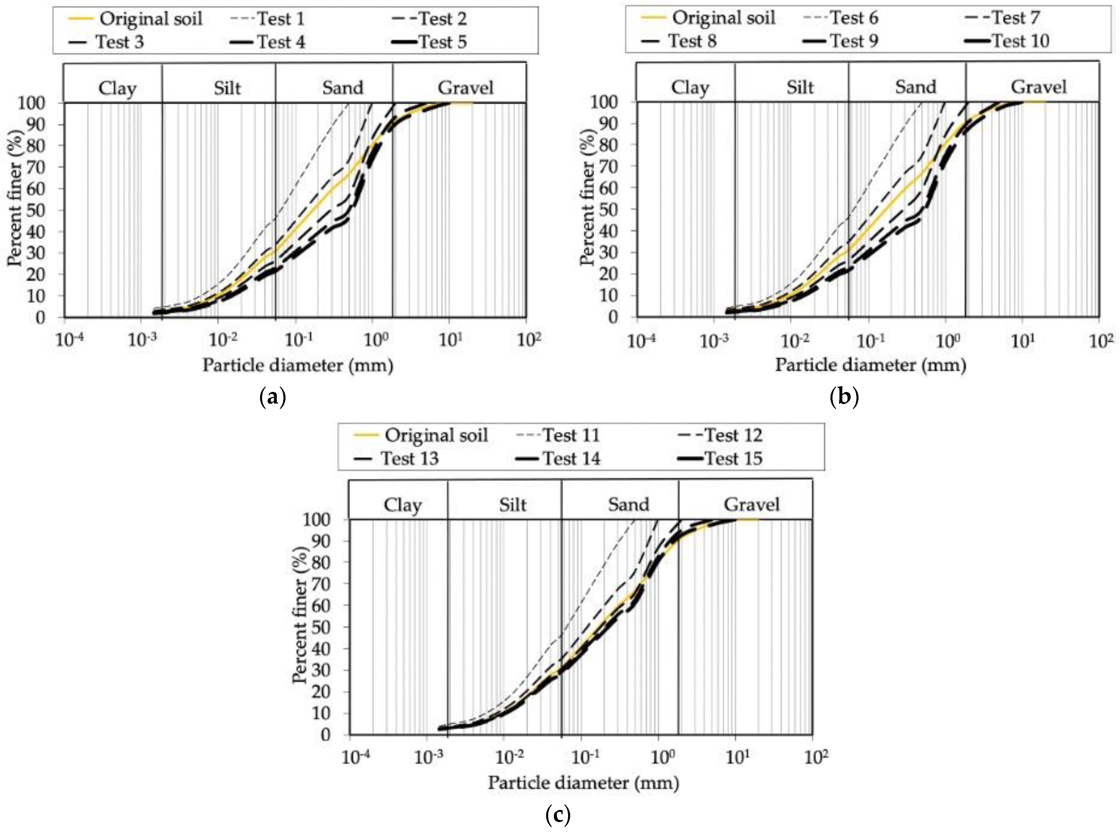
The source areas of the Monteforte Irpino debris flow (which occurred in 1998 in Campania, Italy) provided the soils used to prepare the testing samples. The source areas involve pyroclastic terrains belonging to the deposits generated by volcanic activity. The soils are sandy silt with small clay fraction, having specific gravity GS = 2.57, dry weight of soil per unit volume γd = 7.11 KNm−3, total weight of soil per unit volume γ = 12.11 KNm−3, and porosity p = 0.71. The soils are sandy silt with small clay fraction. Representative threshold sediment size is assumed to be 0.5 mm, which corresponds to the limiting range of medium sand (according to the Wentworth scale). Fine–grained sediment and coarse–grained sediment are defined accordingly, and correspond to a grain diameter finer or coarser than 0.5 mm, respectively. The coarser fraction (i.e., having sediment diameter d > 0.5 mm) is subdivided into four classes: the first two correspond to coarse sand (0.5 mm < d < 1.0 mm) and very coarse sand (1.0 mm < d < 2.0 mm). The latter two (2.0 mm < d < 5.0 mm and 5.0 mm < d < 10.0 mm) correspond to the maximum grain size diameter of the collected samples (see Figure 1).
Before any test, organic elements are removed from the sampled soils and they are dried out in an oven at 104 °C for a day. Then, a mixture of the desired total volumetric concentration ΦT is prepared by mixing the dry, cooled soils, including the chosen fine– and coarse–grained fraction, with an appropriate amount of distilled water. Therefore, the resulting total bulk volume concentration ΦT is:
where Φf and Φg are the solid volumetric concentration for both the fine and coarse–grained mixtures, respectively:
In Equations (1)–(3) the subscripts s, f, g, and w refer to solid, fine–grained, coarse–grained materials and water, respectively. Before starting each test, a sample of about 0.5 10−3 m3 of distilled water and soils is constantly mixed for 15 min at uniform speed (30 rpm at constant temperature of about 23 °C).
To compare different mixtures with different bulk sediment concentrations, it is preferable to use the reduced fraction ΦT/ΦM, where ΦM represents the maximum sediment concentration of the mixture. Even though the actual maximum concentration mainly depends on grain shape and sorting, the proposed model uses a constant value ΦM = 0.64, which corresponds to a close random packing configuration [26].
The inclined plane test (see Table 1) included 14 runs conducted on a mixture of clear water and fine–grained (i.e., mixtures composed of soil fraction with a particle diameter less than 0.5 mm) and coarse–grained suspensions (i.e., mixtures composed of soil fraction with particle diameters ranging up to 10 mm).
The total grain concentration ranged from 25% to 41% in order to include a large variety of conditions under which to evaluate the macro–viscous behaviour of the mixture.
Tests 1–5 correspond to ΦT = 30%, and runs 6–10 were carried out with ΦT = 32%, varying the relative content of fine and coarse grains. In order to investigate the effect of increasing coarse particle content, with the fine fraction constant (Φf = 25%), runs 11–15 were performed using a different concentration of coarse particles Φg.
A typical inclined plane test starts by splitting the suspension on a rough horizontal plane in order to obtain a wide layer of material, and the sample thickness (h0) corresponding to the initial condition at rest is measured at different locations far from the edge (being a distance at least three times the maximum value of h0). Then, the tray is inclined step–by–step until the critical angle (ic) is reached, corresponding to a notable motion of the front edge, and the test goes on until full stoppage of the sliding mass is achieved. Lastly, the thickness (hf) of the deposited mass at rest is measured, following the same procedure used to measure the initial thickness h0. Typically, each test lasted about ten seconds, from the initial spreading to the stoppage of the slurry.
According to the lubrication assumption (i.e., material thickness h0 is much smaller than its longitudinal extent), a uniform flow condition may be assumed for the flow mixture and, disregarding inertial effects, momentum balance provides shear stress distribution within the mixture [27]. Threshold stress corresponding to the start of flowing (τc1) and to the flow stoppage (τc2) can be interpreted as a measure of static and dynamic yield stress, and they are calculated as follows:
where g is the gravitational acceleration and ρ is the density of the fluid. Table 1 reports the experimental programme and the results in terms of static (τc1) and dynamic (τc2) yield stress.
3. Results and Discussion
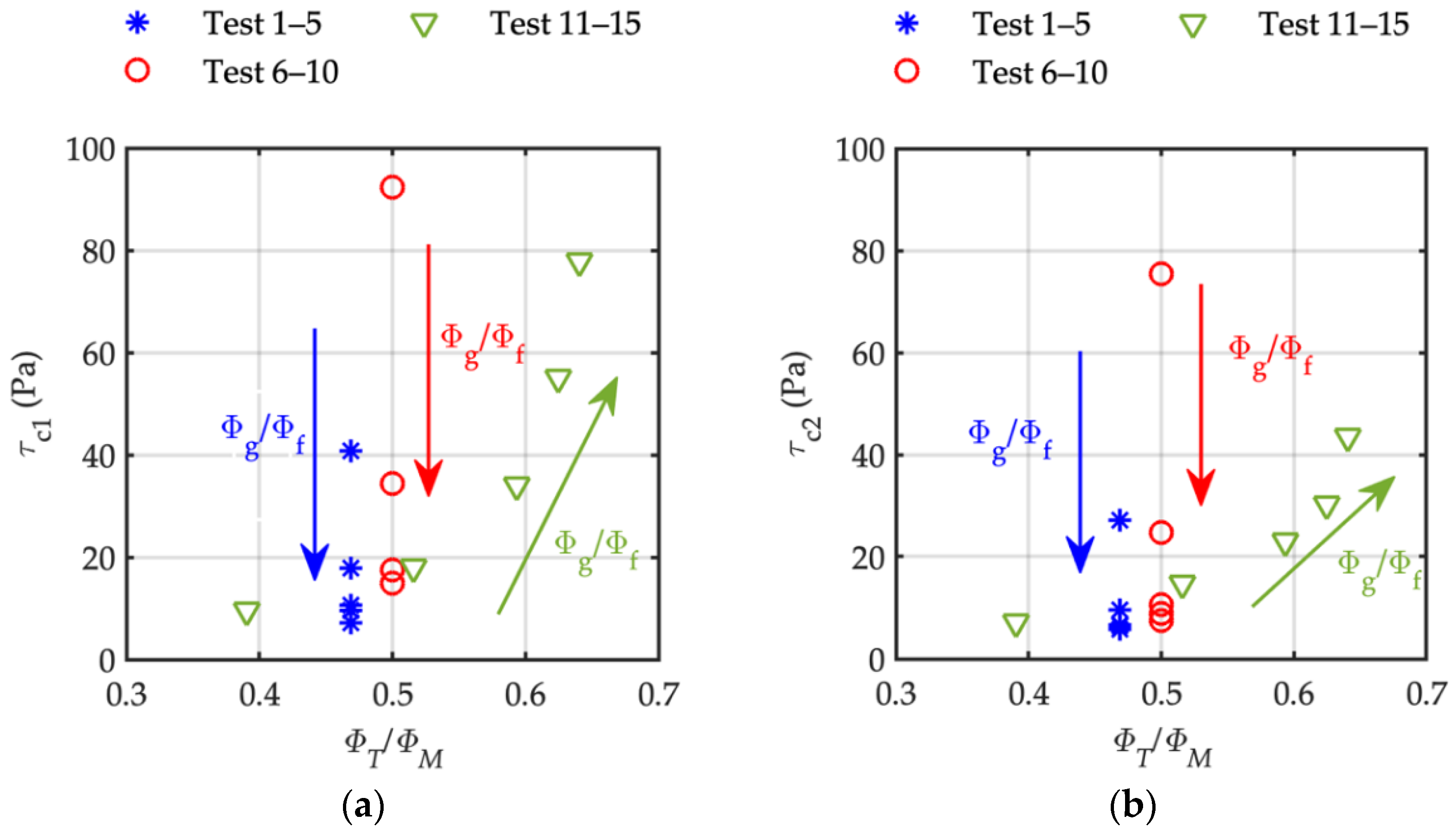
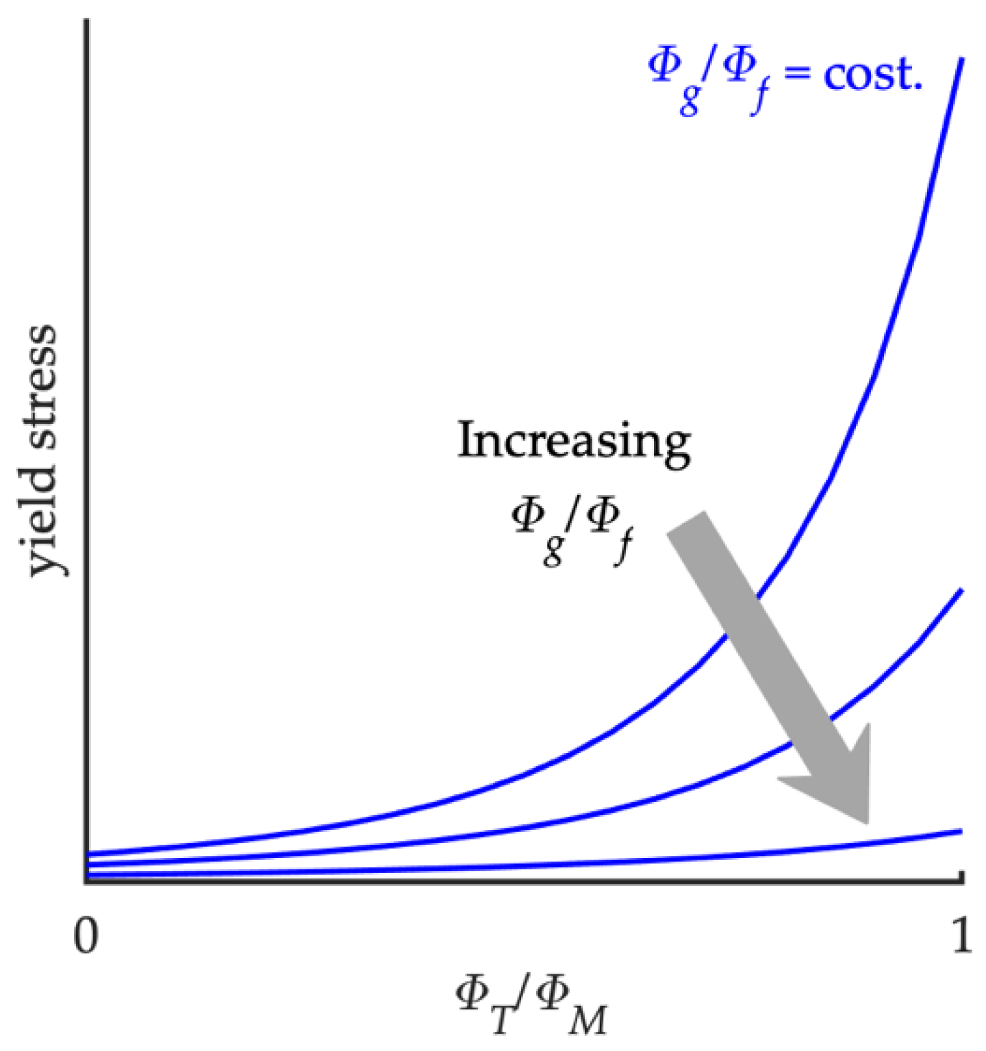
Figure 2 shows that, assuming a fixed reduced bulk sediment fraction, the static and dynamic yields decrease after increasing the coarse–to–fine grain content ratio (see test 1–5 and test 6–10 in Table 1). Thus, we may infer a depletion effect on yield stress curve due to coarse–to–fine content, which flattens the steep enhancing of yield stress associated with increasing reduced sediment fraction, as is qualitatively depicted in Figure 3. Moreover, tests 11–15 show that scaling up bulk concentration leads to a significant enhancement of yield stress, even though the variation in coarse–to–fine sediment content should counterbalance the yield augmentation.
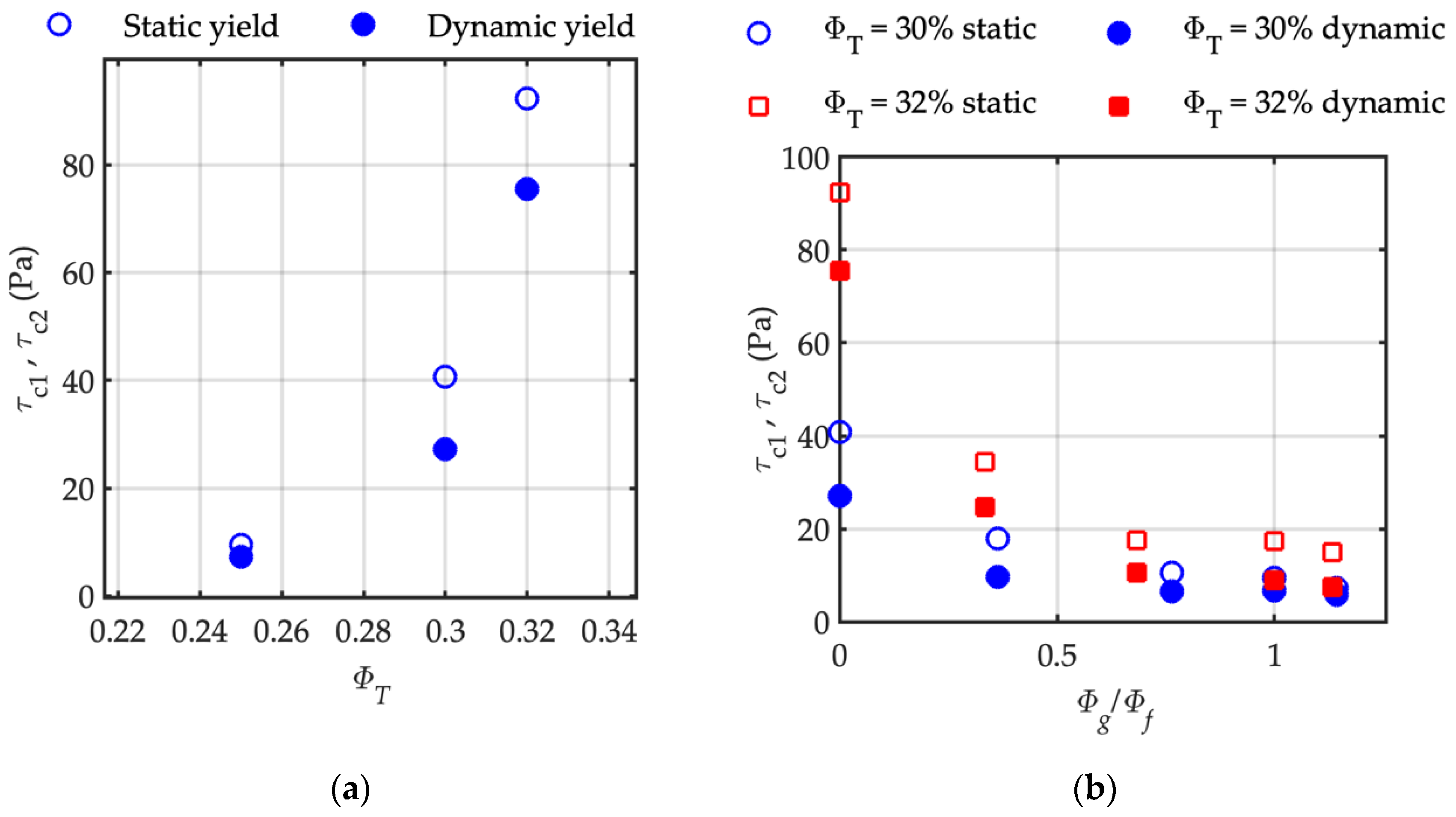
The influence of bulk sediment concentration (at constant coarse–to–fine content) on yield stress may be understood by considering the fine–grained mixture (i.e., Φg/Φf = 0%) plotted in Figure 4a. In fact, increasing grain content leads to a monotonic increase in static and dynamic yield stress, and this is consistent with findings reported by several authors [17,28]. Like Ancey & Jorrot [10], who experimented with poorly graded sand–clay mixture, we found that the variation of yield stress with sediment concentration is pronounced, and no minimum value of the yield is expected with an increasing rate. Considering the estimated yield stress of the kaolin suspension (i.e., 39 Pa) and the granulometric sand sorting (sediment diameter up to 0.3 mm and 1.2 mm) reported by Ancey and Jorrot [10], even the yield stress values seem consistent with the experiments carried out by the authors, which ranged from about 70 Pa to 700 Pa, corresponding to sediment concentrations ranging from 0.27 to 0.55, respectively. Figure 4a suggests asymptotic yield stress behaviour for the solid concentration, approaching a threshold value. Figure 4b shows yield stress as a function of coarse–to–fine grain content in the case of constant bulk sediment concentration (i.e., tests 1–5, ΦT = 30%, and tests 6–10 ΦT = 32%). Static and dynamic yield stresses systematically decreased, increasing the relative amount of the coarse grain fraction. In fact, increasing the relative content of coarse–to–fine sediment up to 50% reduces the yield stress related to fine–grained mixture to 1/3, independently of the total grain concentration, and the yield reduction is more evident when the bulk granular concentration is increased. Figure 4b shows that an asymptotic low yield stress value may be expected, corresponding to very dominant coarse fraction. Moreover, increasing the relative content of coarse grain reduces the difference between static and dynamic yield, and this effect is more relevant given the lower total sediment concentration (ΦT = 30%).
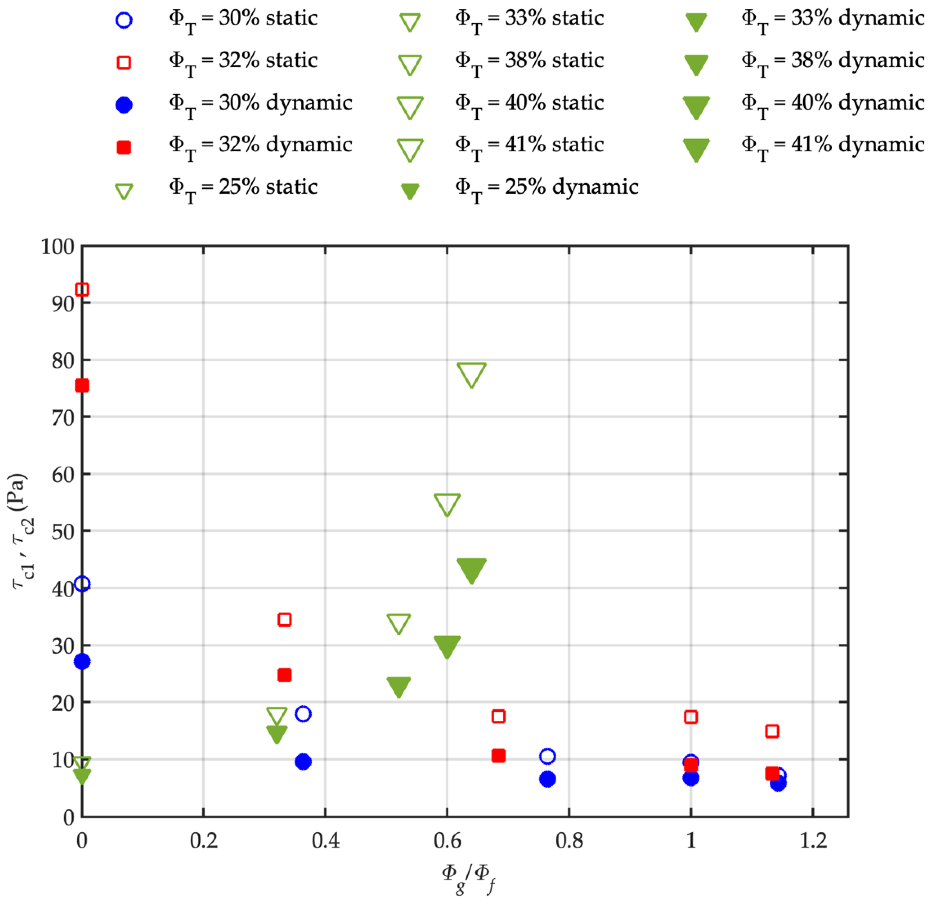
The former behaviour is confirmed even when the whole set of experiments is considered (Figure 5). In this case, the role of the total sediment concentration is also appreciable: the higher the total grain concentration (at a fixed coarse–to–fine grain fraction), the larger the difference between static and dynamic yield. Moreover, the yield stress increases, thus increasing the bulk volume concentration of the mixtures. The fine–grained fraction affects the rheological behavior: increasing the smaller grain content (at a fixed coarse grain fraction) enhances the yield of the slurries, as is shown by a comparison between test 2 (Φf = 22%, Φg = 8%), test 7 (Φf = 24%, Φg = 8%) and test 12 (Φf = 25%, Φg = 8%), where the yield stress more than doubled despite a limited change in fine grain content.
The interpretation of the experimental results plotted in Figure 5 is not trivial. Since yield stress depends considerably on the presence of poorly sorted sediments, it is necessary to consider individual yield value, depending on both bulk concentration and coarse–to–fine grain content. In fact, considering bulk concentration ΦT = (30%, 32%, 33%) and Φg/Φf ≈ (0.36, 0.33, 0.32), the yield stress shows values close to τc1 = (17.9, 34.4, 17.9) Pa, and τc2 = (9.6, 24.8, 14.7) Pa. However, a large range of yield stress results is obtained when ΦT = (40%, 41%), Φg/Φf ≈ (0.64, 0.66).
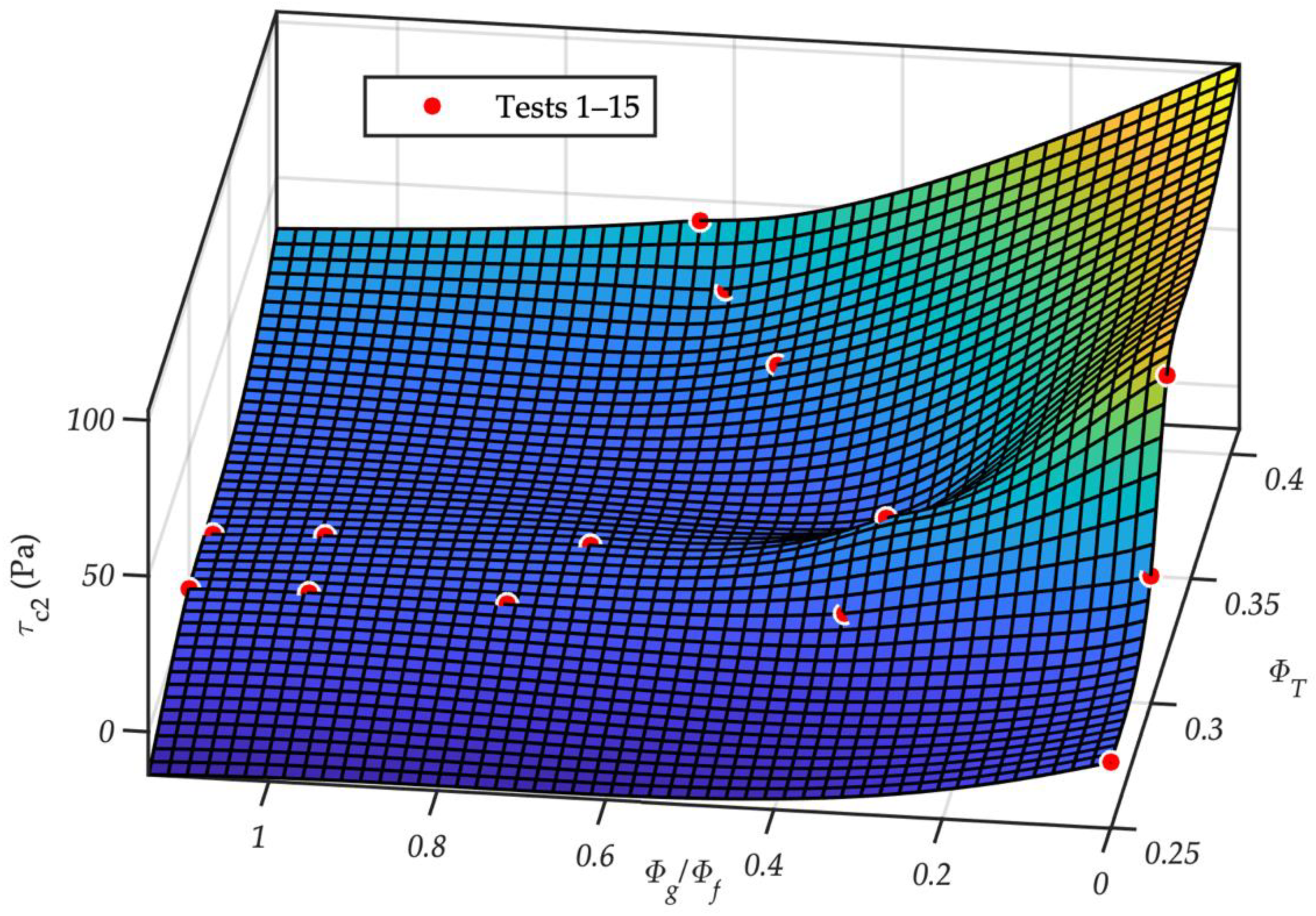
To better understand this behaviour, Figure 6 plots the experimental dynamic yield stress as a function of total grain concentration and the ratio of the coarse–to–fine–graded mixture. The interpolating surface suggests a functional relationship in terms of both total grain concentration (ΦT) and coarse–to–fine grain content (Φg/Φf), confirming that maximum stress corresponds to the higher bulk concentration and the finer graded sample.
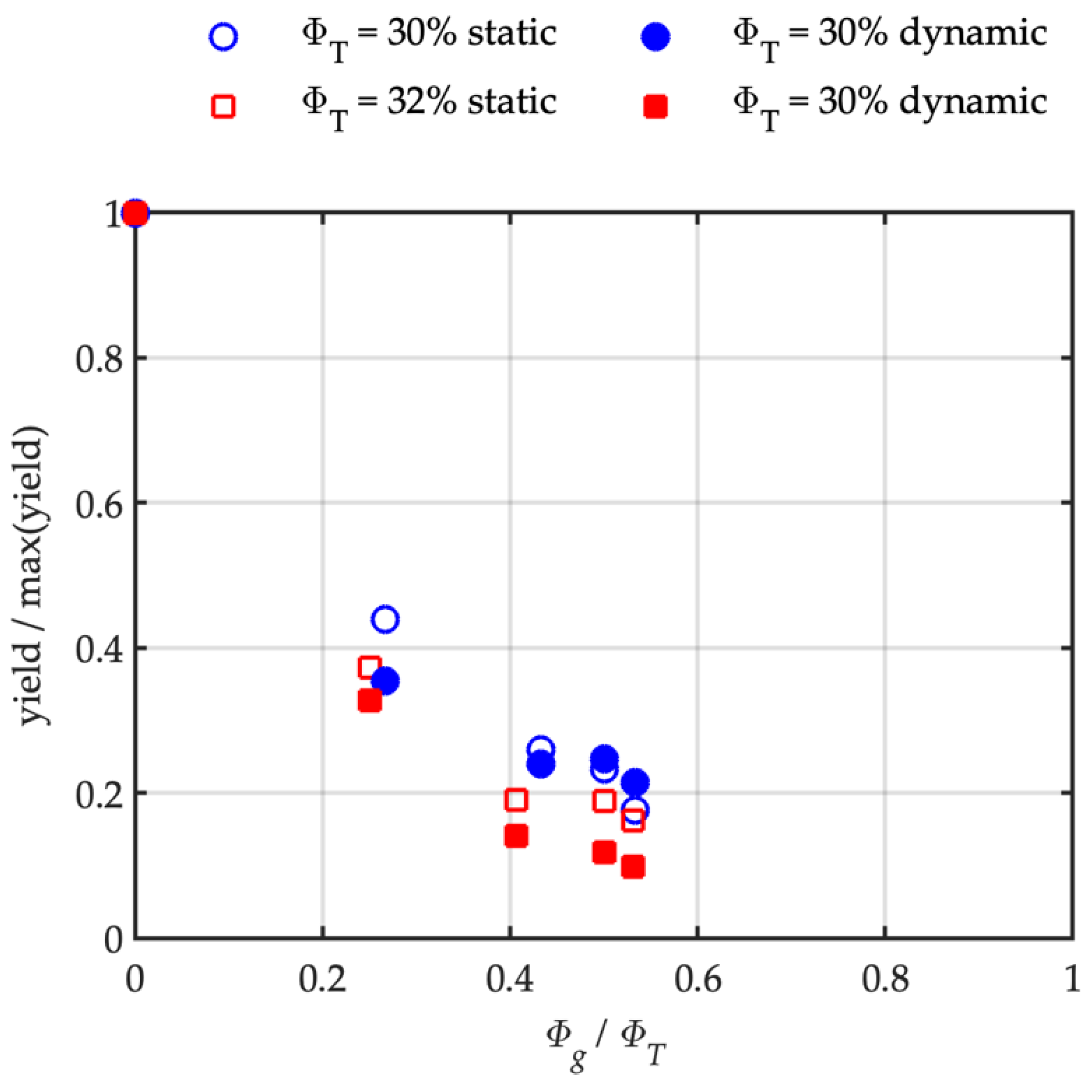
Figure 7 shows static and dynamic yield stress normalised with maximum yield for a fine–grained mixture, , in case of constant bulk concentration ΦT = 30% and ΦT = 32%, as a function of coarse–to–bulk concentration. Both static and dynamic yield markedly reduced when the coarse fraction increased, and the trend is even more evident when the bulk concentration increased. In fact, when it predominates over the finer fraction, the resulting yield is less than about 20% (mixture with ΦT = 30%) or less than 10% (mixture with ΦT = 32%) of the yield stress for the fine–graded mixture (Φg = 0).
Interestingly, for the lowest bulk concentration ΦT = 30%, the static and dynamic yield trend towards the same value if the proportion of coarser particles is increased until it is comparable to or dominant over the finer fraction, as it is also evident from Figure 5. However, for a higher bulk concentration ΦT = 32%, static and dynamic yield still show different values, even if the coarser fraction is dominant. Remarkably, in the latter case the dynamic yield is comparable to the yield stress of the mixture with ΦT = 30% (Figure 5).
It may be argued that the presence of the finer fraction not only epitomises the pseudo–viscous behaviour of the flowing mixture [2], but even increases the yield stress (Figure 4a). The higher the concentration, the greater the difference between static and dynamic yield. Conversely, the presence of coarse fraction tends to reduce the yield stress irrespective of bulk concentration, and when coarse sediment is the dominant content, the dynamic yield is almost independent of coarse–to–fine sediment content and of sediment bulk concentration (Figure 4b; ΦT = 30% and ΦT = 32%).
Experiments involving reconstituted debris flow samples highlight the importance of grain concentration in determining yield stress. The presence of coarse graded sediments affects the rheological behaviour, and significantly reduces yield stress. The finer graded matrix content increases the yield stress, whereas the presence of a coarser component reduces the threshold stress. Therefore, increasing relative coarse–to–fine content counteracts the effects of increasing bulk concentration in terms of the resulting yield stress. Consequently, defining a yield stress model is not a trivial matter for natural slurries where grains are always poorly sorted, and its dependence on grain sorting is of great relevance when dealing with natural slurries. From now on, in order to illustrate the model, we will focus on dynamic yield stress, which will now be referred as yield stress.
4. The Model
4.1. Previous Yield Models
The literature describes different experimental models for yield stress as a function of sediment concentration in viscous granular flow mixtures and muddy sediments slurries. However, few models appear to refer to yield stress determined by natural poorly sorted sediment, typical of the natural debris flow matrix.
Migniot [29] experimented with several different soil–water mixtures that had a sediment diameter of less than 0.3 mm, and were of fluvial, estuarine, marine, lacustrine, mining, and artificial origin. He established the following power law:
where exponent b = 4–5, and coefficient a depend on the soil characteristics. Later, Pantet et al. 2010 successfully applied the same power law with exponent b = 3, in testing muddy sediments from Marennes Oleron Bay (even though their experiments show a significant scatter of data). Mahaut et al. [30] tested polystyrene and glass beads in various bentonite suspensions, emulsions, and Carbopol gel, and their results were a remarkably good fit to the following law (consistent with Krieger–Dougherty’s law [31]):
where τco represents the yield stress corresponding to the viscous interstitial fluid, and ΦM = 0.57 was set up to fit experimental data.
Wildemuth and Williams [8] considered non–interacting particle suspensions of Illinois coal (grain diameter less than 0.120 mm) in water–glycerol, bromonaphthalene, and Aroclor suspending fluids. They found that the yield stress was a consequence of the maximum solid concentration on the shear stress, and they proposed an empirical relationship based on the limiting values of total sediment concentration, which implies the existence of yield stress (i.e., Φ0 < ΦT < Φ∞) and fitting parameters K and m:
Ancey & Jorrot [10] experimented with a glass bead suspension within a water–kaolin dispersion, and they successfully applied an extension of Wildemuth and Williams [8] model:
where Φk is kaolin concentration, τk is the yield stress of the water–kaolin dispersion, and , m are fitting parameters.
A rather complicated relationship was proposed by Yu et al. [15] after testing water–clay mixtures at different sediment concentrations, and using various clay types:
where c1, c2, are empirical coefficients, is an empirical function fitting experimental data, is equivalent solid concentration derived from volumetric solid concentration ΦT and sediment gradation, and P is the equivalent percentage of clay minerals (in case of mixed clays). Moreover, threshold concentration values Φk = [0.47; 0.59] (the values and definition of which were not backed by any evidence from the authors) were introduced to differentiate the fitting function .
A simpler model was proposed by O’Brien and Julien [17], who tested mudflow matrices (i.e., silt–clay–water mixture) derived from natural mudflow deposits in the central Colorado Rocky Mountain, and muddy sediment slurries comprising silts and clays (up to a concentration of 5% in volume), and fine–to–medium sands (up to a concentration of 35% in volume):
where , are constant empirical coefficients depending on the material. In effect, the authors reported a significant change in the rheological properties of the matrix, associated with sand content exceeding a volume concentration of 20%.
4.2. The Proposed Yield Model
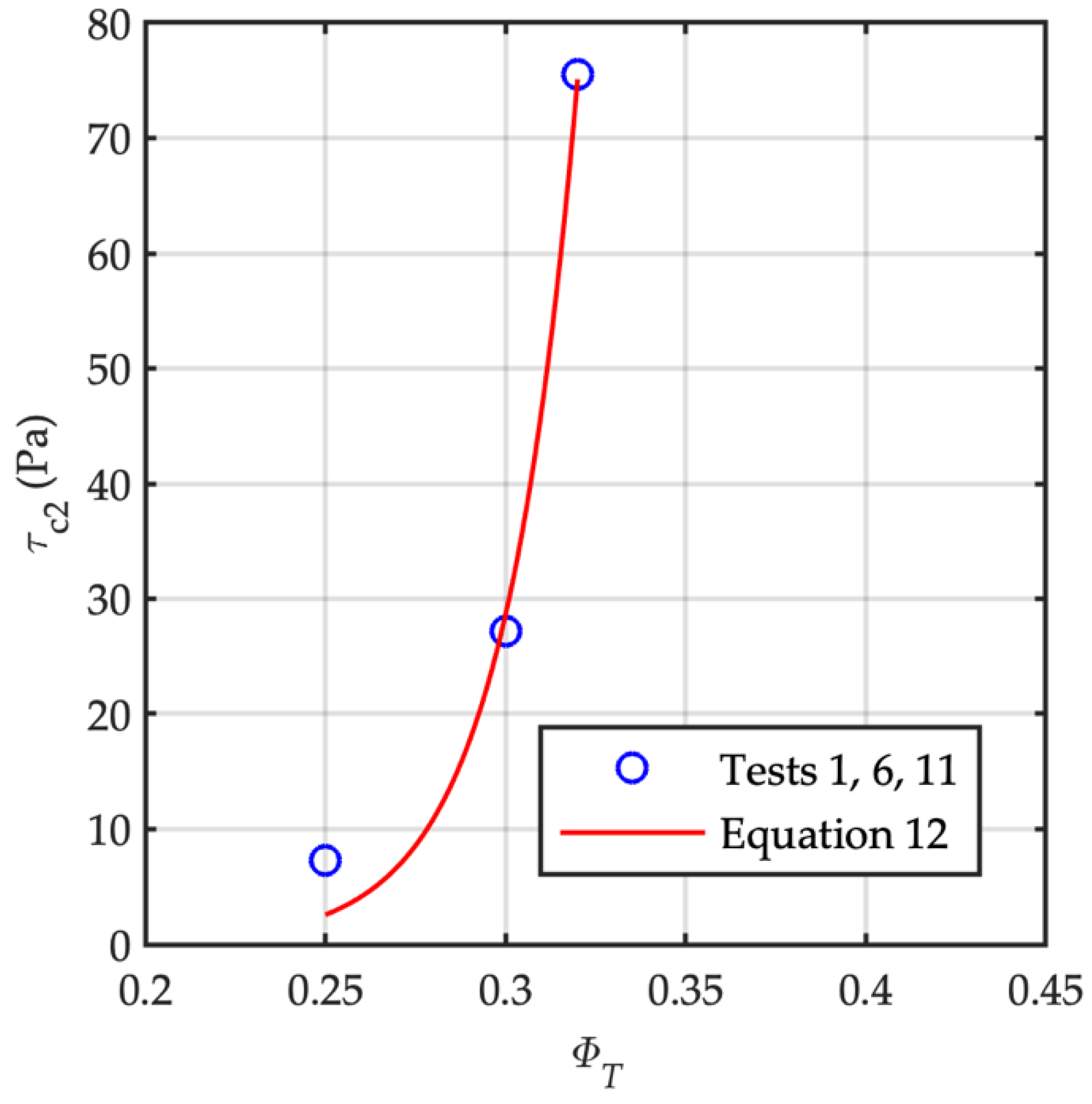
Considering fine–graded sediment mixtures in water (i.e., Φg/Φf = 0; tests 1, 6, and 11 in Table 1 and Figure 4), yield stress (both static and dynamic) may be considered a power function of bulk sediment concentration ΦT:
For a fine–grained mixture (i.e., Φg/Φf = 0), fitting tests 1, 6, and 11 (corresponding to ΦT = 30%, 32%, and 25% respectively), give the results = 1.5 × 10⁻⁵ Pa and β = 48.2 (Figure 8), which are consistent with values empirically determined by Major and Pearson [28], whereas they are on the border of the range suggested by Sosio and Crosta [11], and O’Brien and Julien [17] who experimented with mixtures of sand added to silt–clay dispersions, and the large scatter of parameter values may be partially explained by the difference in materials.
In fact, the general behaviour of yield stress reported in Figure 6, shows α and β to be a function not only of bulk grain concentration, but also of relative coarse–to–fine–graded sediment content, which is not taken into consideration in Equation (12). Therefore, a functional relationship between coefficients and and coarse–to–fine sediment content (Φg/Φf) and the bulk sediment concentration (ΦT) is introduced, assuming asymptotic behaviour of a Newtonian fluid in the case of pure water , and no flow–like behaviour for the maximum (theoretical) sediment concentration ΦM, . To compare different mixtures with different bulk sediment concentration, it is preferable to use the reduced fraction ΦT/ΦM:
As a first approximation, is considered:
where is the grading function of the relative content of coarse–to–fine grains. Its value depends on mixture characteristics, and it can be obtained by fitting the experimental data, thus Equation (12) becomes:
Despite the actual maximum concentration, ΦM mainly depends on grain shape and sorting. The proposed model uses ΦM = 0.64, which corresponds to a close random packing configuration [27].
4.3. Application of the Proposed Yield Model in Case of Fine–Grained Mixtures
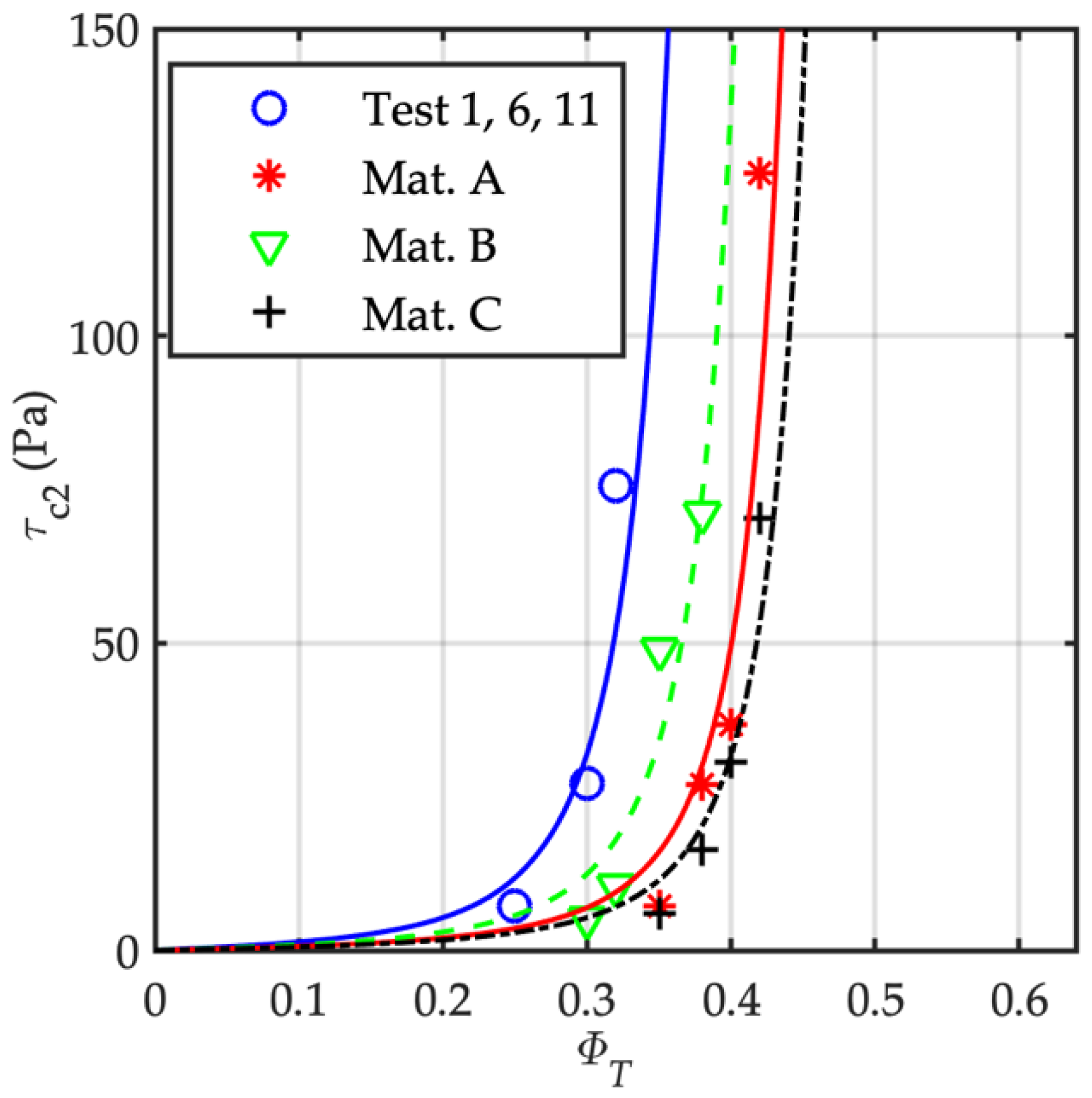
As a first step, Equation (15) is validated considering the limiting case of fine–grained mixtures. Different experiments reported in Scotto di Santolo et al. [32] are considered for this purpose as well as the experiments on fine–grained mixtures reported in Table 1 (i.e., Tests 1, 6 and 11). Table 2 lists the data–set of 15 experiments. They refer to fine–grained (sediment diameter d < 0.5 mm) samples of reconstituted debris flow deposits from a source debris flow area in the Campania region (Italy). One of them was collected in Monteforte Irpino, the same area as the samples listed in Table 1, and the other two came from Nocera and Astroni. All of them are pyroclastic; the Monteforte Irpino (material A) and Nocera (material B) deposits derive from the activity of Monte Somma/Vesuvius, whereas Astroni (material C) deposits derive from volcanic activity in the Phlegrean Fields close to Naples. Soil A and soil B are sandy silt with a small clay fraction, soil C is gravelly–silty sand. Soil characteristics are detailed in [32]. Test samples and inclined plane tests were prepared and carried out as already described in Section 2. All of the water–sediment mixtures included grain sizes of under 0.5 mm, and four mixtures with different sediment concentrations were tested for every soil. In case of fine–grained samples, the resulting grading function is:
and its value is estimated by fitting experimental results. Figure 9 shows good agreement between the proposed model Equation (15) and all the fine–grained mixtures considered. Table 2 shows the measured static and dynamic yield stress, and the best fitting value of according to Equation (15).
4.4. Application of the Proposed Yield Model to Coarse–Grained, Poorly Sorted Mixtures
The whole set of experiments in Table 1, involving fluid–granular mixtures having different grain class ranging from silty sand to fine pebbles, was considered in order to show the performance of model Equation (15) for coarse–grained, poorly sorted mixtures.
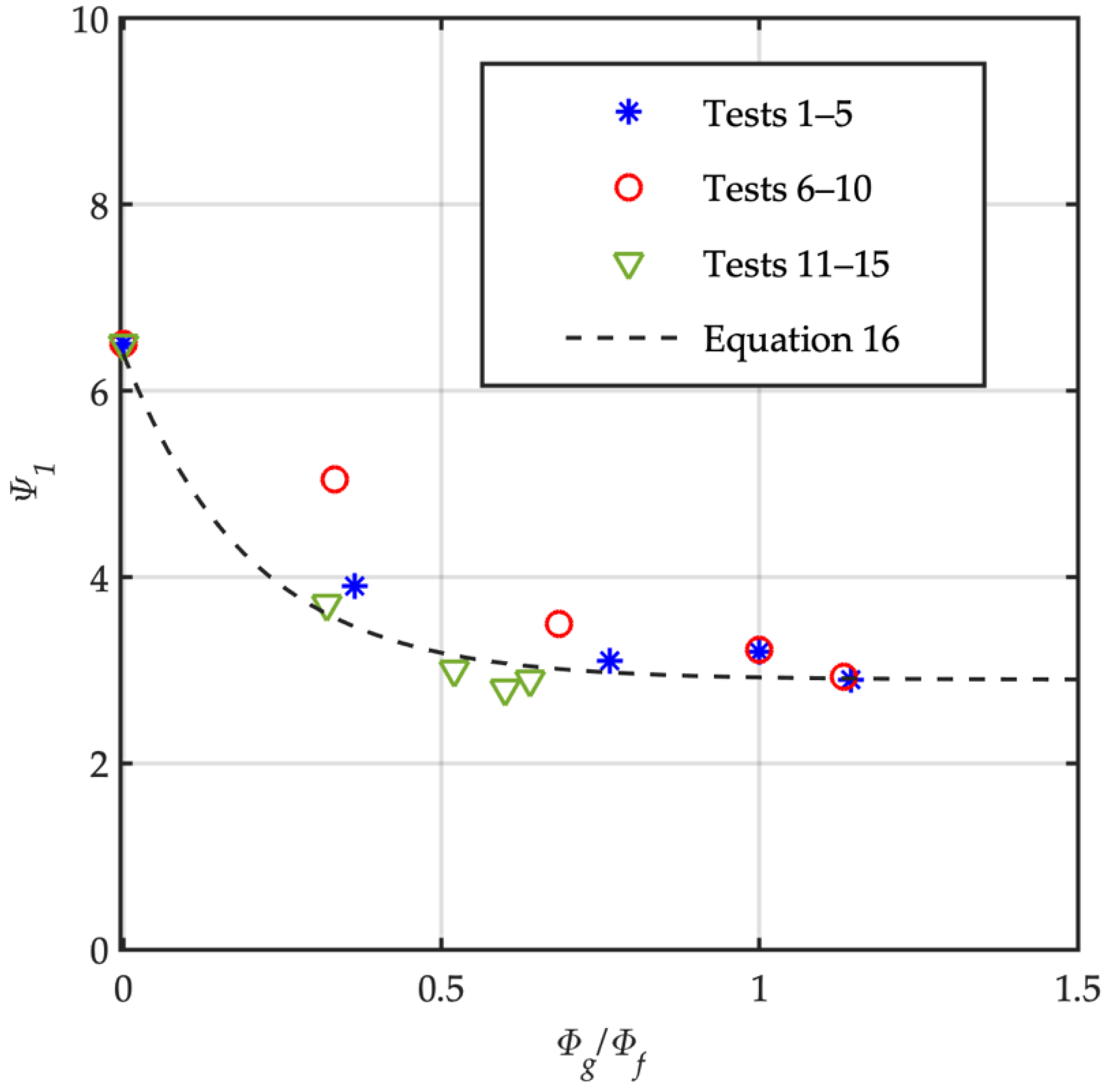
Equation (15) was applied, and for each test the best fitting value of was estimated according to the related Φg/Φf value. Figure 10 shows the estimated value of coefficient as a function of coarse–to–fine concentration Φg/Φf, and the best fitting function :
where k1, k2 and k3 are empirical coefficients depending on the material. In this case k1 = 3.5, k2 = −5 and k3 = 2.9 are assumed.
Figure 10 clearly shows that the grading function is almost constant for > 0.5, which would suggest that for relatively coarse–grained mixtures the yield stress depends predominantly on bulk sediment concentration (see Equation (15)). In fact, the large proportion of coarser grains suggests that the yield stress is mainly affected by frictional contact between the particles, and the role of the interstitial viscous fluid is reduced. Similarly, for dominant fine–grained content, the exponential increase of yield stress with sediment concentration, (Figure 9), confirms the relevance of interparticle collisions and frictional stress in halting the flowing slurries.
4.5. Model Performance and Its Main Features
Figure 11a shows the performance of the proposed model (Equation (15) ∧ Equation (17)) comparing modelled and measured values for the entire set of data referring to bulk sediment concentration (0.3; 0.41) and coarse–to–fine content (0; 0.143). Most of the modelled yield stress falls into the ±25% confidence range, showing a favourable agreement between the model and the experiments. Figure 11b depicts the 3–D graph of the proposed yield stress model, showing most of the experimental points lying on the resulting yield stress area.
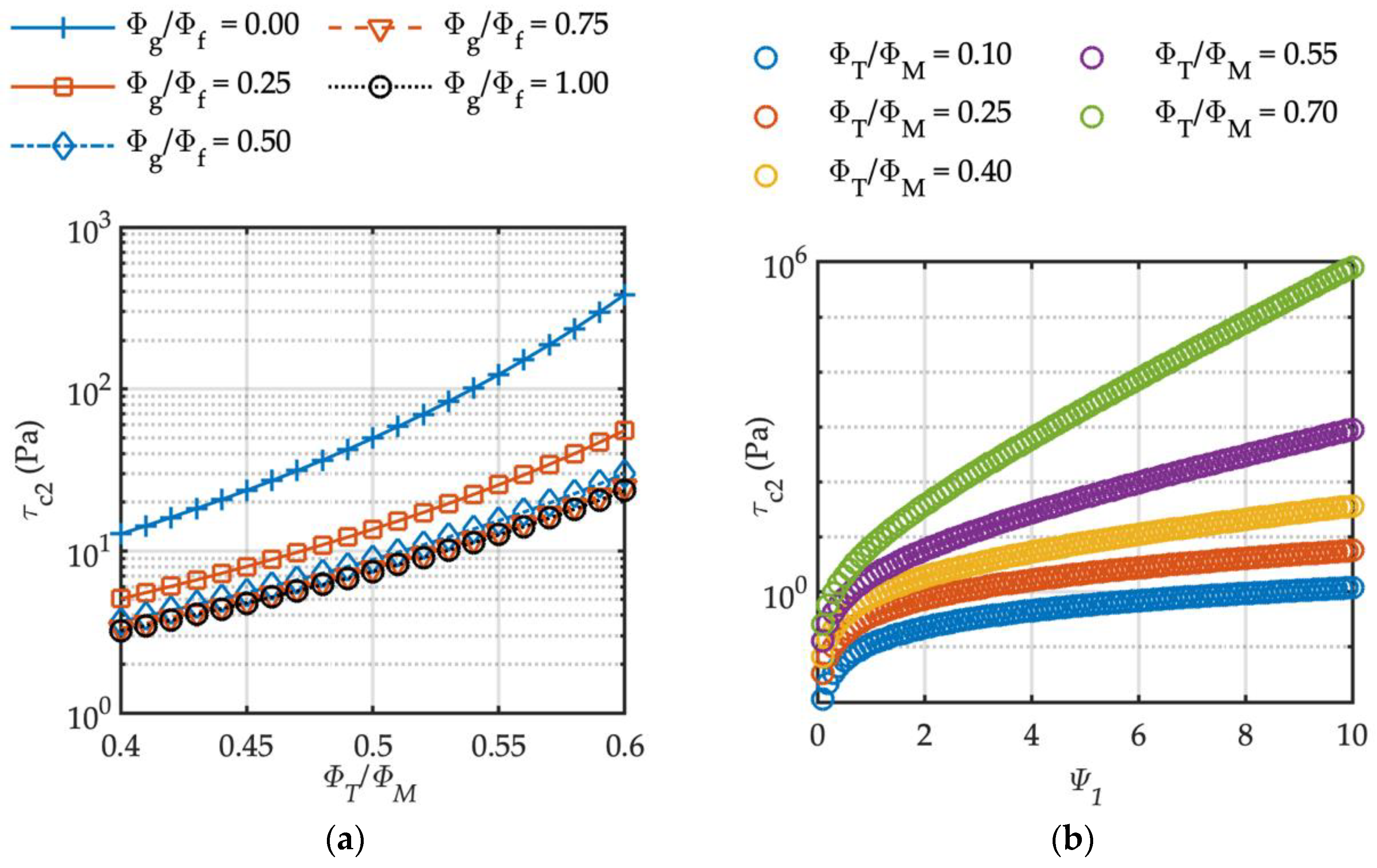
Figure 12a plots the yield stress model results as a function of relative bulk sediment concentration in the case of different coarse–to–fine–graded mixtures. A concentration range comparable to that of the present experiments is considered, and in Equation (17) the fitting coefficients are set as k1 = 3.5, k2 = −5 and k3 = 2.9, according to the experimental results considered in this case. Interestingly, for a large proportion of coarse grain (namely Φg/Φf > 0.5), the yield stress was found to be almost independent from the coarse–to–fine grain fraction. Conversely, fine–grained mixtures show a yield stress higher by one order of magnitude than those calculated for cases where the coarse sediment content was dominant over the finest fraction. Thus, the larger bulk concentration leads to a noticeable increase in the yield stress, and this enhancement is more pronounced for fine–grained mixtures than for slurries with a significant content of coarser particles.
Figure 12b depicts the yield stress obtained by applying the model as a function of grading function , assuming different reduced fraction values ΦT/ΦM. Grading function essentially depends on the application of empirical parameters k1, k2 and k3 (see Equation (17)) which depend on mixture characteristics. In the experiments considered here, ranges from 6.5 to 2.8 (see Figure 10). In the range of 0 < < 10, corresponding to a coarse–to–fine ratio of less than 0.25, the yield stress varies by one order of magnitude (i.e., 1 < τc2 < 10), whereas it increases by several orders of magnitude for Φg/Φf > 0.4. Thus, poorly graded slurries having a relatively low content of coarse fraction are less sensitive to empirical fitting parameters (i.e., k1, k2 and k3).
It is worth considering the proposed model (Equations (15) and (17)) in the case of fine–grained mixtures (i.e., Φg/Φf = 0), in which case the Equation is reduced to:
The value of can be estimated directly from the experimental results (see Figure 9 and Table 2). In this way, the fitting parameters are reduced to only one () instead of two, as it is in the case of the widely used power function model (Equation (6)) and exponential function model (Equation (10)).
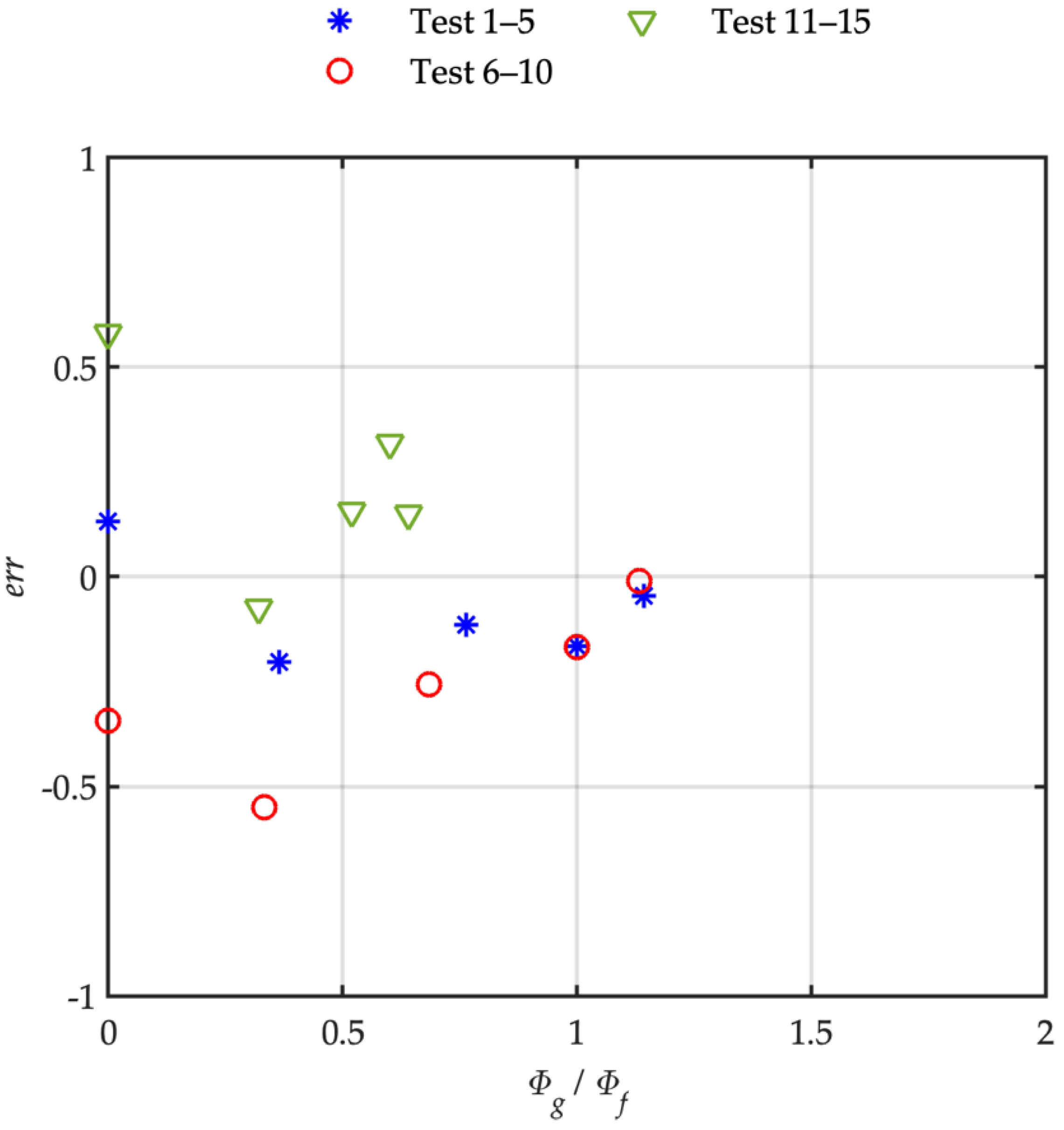
The variation rate of grading function depends significantly on coarse–to–fine content Φg/Φf = 0 when the coarse fraction is relatively low, e.g., 0 < Φg/Φf < 0.5 (see Figure 10). Hence, to correctly fit the grading function it is important to test samples corresponding to low values of coarse–to–fine sediment ratio, specifically including fine–grained mixtures. This reflects the reliability of the model, as it is evident from Figure 13 where the model error is depicted:
where is the modelled yield stress. In fact, the reliability of the model significantly increases with increasing coarse–to–fine content. The model performs best for poorly sorted mixtures, let us say Φg/Φf > 0.75. It may be argued that this is a consequence of the assumption in Equation (12), which leads to an attractive simplification in the proposed yield stress modelling. However, the lower sediment concentration for the fine–grained mixtures (see Figure 9b) also affects the model. Indeed, several authors [11,17,28] have suggested an empirical power function of bulk sediment concentration ΦT (Equation (11)) with constant empirical soil coefficients, unlike the proposed model where soils coefficients are a function of coarse–to–fine grain content and bulk sediment concentration (Equation (14)). Nonetheless, the results shown in Figure 11a,b, are considered satisfactory in view of the relative simplicity of the model.
In summary, to apply the proposed model to poorly graded viscous slurries based on experimental investigations, the laboratory tests should consider samples of different coarse–to–fine sediment content, even including only fine–grained mixtures. Then the model setting follows the ensuing steps:
- 1.
- The measured yield stress of fine–grained slurries (Φg/Φf = 0) is considered, and the model (Equation (18)) is applied. Then the best fitting value of the grading function is estimated.
- 2.
- Yield stress corresponding to slurries with different values of coarse–to–fine sediment content (Φg/Φf ≠ 0) is considered. The model (Equation (15)) is applied, and the best fitting grading function values (Φg/Φf) are estimated.
- 3.
- The resulting values (Φg/Φf) are used to fit the empirical parameters k1, k2 and k3 in the grading function Equation (17), to be used for setting up the yield stress model.
The model has been applied to poorly sorted natural sediment–water mixtures. Sediments were split in five classes, defined on the basis of the sieve dimensions, and into two categories: fine–grained (d < 0.5 mm) and coarse–grained (d > 0.5 mm). Even though the coarse–grained mixtures were prepared by mixing different percentages of each class belonging to the coarse–grained category, at this stage the model does not distinguish between the different coarse–grained classes content, but considers the whole percentage of the coarse–to–fine ratio present in the slurry. Nonetheless, the results are encouraging (Figure 11). It would be interesting to enhance the model, distinguishing between the different sediment classes present in the slurries or, even better, using the characteristics parameters representing the granulometric curve of natural sediments.
5. Conclusions
The experiments on poorly graded natural sediment mixtures show that the yield stress depends a great deal on bulk–solid concentration and on coarse–to–fine sediment content. Therefore, it is not possible to apply any model predicting yield stress behaviour based on bulk sediment concentration alone.
According to the experimental results, the larger bulk concentration leads to a significant increase in the yield stress value, and this boost is more evident for finer grained mixtures. Static and dynamic yield significantly reduced increasing coarse fraction, and the higher the bulk sediment concentration the more evident the effect.
Even the ratio between static to dynamic yield stress is affected by the presence of coarse particles, and static to dynamic yield shows different behaviour depending on the bulk sediment concentration of the mixture. The higher the concentration, the greater the difference between static and dynamic yield.
The proposed yield-stress model introduces a grading function which considers the coarse–to–fine grain fraction, fitted based on the mixture characteristics. The variation rate of grading function significantly depends on coarse–to–fine content. The lower the coarse grain presence, the higher the function rate. The model performance is satisfactory, and its reliability increases in the case of higher coarse grain content.
In the case of dominant coarse grain content (namely Φg/Φf > 0.5), the yield stress was found to be almost independent of the coarse–to–fine grain fraction, and its value is lower by one order of magnitude than those calculated for fine–grained mixtures. Further investigations may be oriented towards analysing the effects of splitting in different sediment size classes present in the slurry or using characteristic parameters representing the granulometric curve of natural sediments.
Funding
This research received no external funding.
Institutional Review Board Statement
Not applicable.
Informed Consent Statement
Not applicable.
Acknowledgments
The author thanks Anna Maria Pellegrino for the experimental data.
Conflicts of Interest
The author declares no conflict of interest.
References
- Pellegrino, A.M.; Schippa, L. Rheological modeling of macro viscous flows of granular suspension of regular and irregular particles. Water 2017, 10, 21. [Google Scholar] [CrossRef] [Green Version]
- Schippa, L. Modeling the effect of sediment concentration on the flow–like behaviour of natural debris flow. Int. J. Sediment Res. 2020, 35, 315–327. [Google Scholar] [CrossRef]
- Contreras, S.M.; Davis, T.R.H. Coarse grained debris–flow hysteresis and time dependent rheology. J. Hydraul. Eng. ASCE 2000, 126, 934–941. [Google Scholar] [CrossRef]
- Schatzmann, M.; Fischer, P.; Bezzola, G.R. Rheological behaviour of fine and large particle suspensions. J. Hydraul. Eng. ASCE 2003, 129, 796–803. [Google Scholar] [CrossRef]
- Pellegrino, A.M.; Schippa, L. Macro viscous regime of natural dense granular mixtures. Int. J. GEOMATE 2013, 4, 482–489. [Google Scholar] [CrossRef]
- Pellegrino, A.M.; Di Santolo, A.S.; Schippa, L. The sphere drag rheometer: A new instrument for analysing mud and debris flow materials. Int. J. GEOMATE 2016, 11, 2512–2519. [Google Scholar] [CrossRef]
- Jomha, A.I.; Merrington, A.; Woodcock, L.V.; Barnes, H.A.; Lips, A. Recent developments in dense suspension rheology. Powder Technol. 1990, 65, 343–370. [Google Scholar] [CrossRef]
- Wildemuth, C.R.; Williams, M.C. A new interpretation of viscosity and yield stress in dense slurries: Coal and other irregular particles. Rheol. Acta 1985, 24, 75–91. [Google Scholar] [CrossRef]
- Kytomaa, H.K.; Prasad, D. Transition from quasi static to rate dependent shearing of concentrated suspensions. In Powders & Garins 93, Proceedings of the 2nd International Conference on Michromechanics of Granular Media, Birmingham, UK, 12–16 July 1993; Thornton, C., Ed.; Balkema: Rotterdam, The Netherlands, 1993. [Google Scholar]
- Ancey, C.; Jorrot, H. Yield stress for particle suspensions within a clay dispersion. J. Rheol. 2001, 45, 297–319. [Google Scholar] [CrossRef]
- Sosio, R.; Crosta, G.B. Rheology of concentrated granular suspensions and possible implication for debris flow modeling. Water Resour. Res. 2009, 45, W03412. [Google Scholar] [CrossRef] [Green Version]
- Schippa, L.; Doghieri, F.; Pellegrino, A.M.; Pavesi, E. Thixotropic Behavior of Reconstituted Debris–Flow Mixture. Water 2021, 13, 153. [Google Scholar] [CrossRef]
- Pellegrino, A.M.; Schippa, L. A laboratory experience on the effect of grains concentration and coarse sediment on the rheology of natural debris–flows. Environ. Earth Sci. 2018, 77, 1–13. [Google Scholar] [CrossRef]
- Yu, B.; Ma, Y.; Qi, X. Experimental study on the influence of clay materials on the yield stress of debris flows. J. Hydraul. Eng. ASCE 2013, 139, 364–373. [Google Scholar] [CrossRef]
- Yu, B.; Chen, Y.; Liu, Q. Experimental study on the influence of coarse particle on the yield stress of debris flows. App. Rheol. 2016, 26, 42997. [Google Scholar] [CrossRef]
- Pantet, A.; Robert, S.; Jarny, S.; Kervella, S. Effect of Coarse Particle Volume Fraction on the Yield Stress of Muddy Sediments from Marennes Oléron Bay. Adv. Mater. Sci. Eng. 2010, 2010, 245398. [Google Scholar] [CrossRef] [Green Version]
- O’Brien, J.S.; Julien, P.Y. Laboratory analysis of mudflow properties. J. Hydraul. Eng. ASCE 1988, 114, 877–887. [Google Scholar] [CrossRef] [Green Version]
- Jeong, S.W. Grain size dependent rheology on the mobility of debris flows. Geosci. J. 2010, 14, 359–369. [Google Scholar] [CrossRef]
- Chen, H.; Lee, C.F. Runout analysis of slurry flows with Bingham model. J. Geotech. Geoenviron. 2002, 128, 1032–1042. [Google Scholar] [CrossRef]
- Coussot, P.; Piau, J.M. A large–scaled field concentric cylinder rheometer for the study of the rheology of natural coarse suspensions. J. Rheol. 1995, 39, 105–124. [Google Scholar] [CrossRef]
- Banfill, P.F.G. The influence of fine materials in sand on the rheology of fresh mortar. In Proceedings of the International Conference on Utilizing Ready Mix Concrete and Mortar; Dundee, UK, 8–10 September 1999, Dhir, R.K., Limbachiya, M.C., Eds.; Thomas Thelford: London, UK, 1999; pp. 411–420. [Google Scholar]
- Fei, X.; Zhu, P. The viscous debris flow and its determination method. J. Railw. Eng. Soc. 1986, 4, 9–16. (In Chinese) [Google Scholar]
- Wan, Z.; Qian, Y.; Yang, W. The experimental study on hyper concentrated sediment flow. Yellow River. 1979, 1, 5–6. (In Chinese) [Google Scholar]
- Tang, C. The calculating model of yield stress of slurry. J. Sediment Res. 1981, 2, 60–65. (In Chinese) [Google Scholar]
- Jan, C.D.; Yang, C.Y.; Hsu, C.K.; Dey, L. Correlation between the slump parameters and rheological parameters of debris flow. In Debris–Flow Hazards and Mitigation: Mechanics, Monitoring, Modeling and Assessment, Proceedings of the 7th International Conference on Debris–Flow Hazards Mitigation, Golden, CO, USA, 10–13 June 2019; Kean, J.K., Coe, J.A., Santi, P.M., Guillen, B.K., Eds.; Association of Environmental and Engineering Geologists Special Publication 28: Brunswick, OH, USA, 2019. [Google Scholar]
- Meakin, P.; SkJeltorp, A.T. Application of experimental and numerical models to the physics of multiparticle systems. Adv. Phys. 1993, 42, 1–127. [Google Scholar] [CrossRef]
- Coussot, P. Rheometry of Pastes, Suspensions and Granular Materials: Application in Industry and Environment; John Wiley and Sons Inc.: New York, NY, USA, 2005. [Google Scholar]
- Major, J.J.; Pierson, T.C. Debris flow rheology: Experimental analysis of fine–grained slurries. Water Resour. Res. 1992, 38, 841–857. [Google Scholar] [CrossRef]
- Migniot, C. Etude des proprietes physiques de differents sediments tres fins et de leur comportament sous de actions hydrodynamiques. Houille Blanche 1968, 7, 591–620. (In French) [Google Scholar] [CrossRef] [Green Version]
- Mahaut, F.; Chateau, X.; Coussot, P.; Ovarlez, G. Yield stress and elastic modulus of suspensions of noncolloidal particles in yield stress fluids. J. Rheol. 2008, 52, 287. [Google Scholar] [CrossRef] [Green Version]
- Krieger, I.M.; Dougherty, T.J. A Mechanism for Non–Newtonian Flow in suspensions of Rigid Spheres. J. Rheol. 1959, 3, 137. [Google Scholar] [CrossRef]
- Scotto di Santolo, A.M.; Pellegrino, A.M.; Evangelista, A.; Coussot, P. Rheological behaviour of reconstituted pyroclastic debris flow. Geotechnique 2012, 62, 19–27. [Google Scholar] [CrossRef]
Figure 1.
Grain size distribution of the original soil, and of the reconstituted mixtures used for the experimental tests: (a) Test 1–5 ΦT = 30%; (b) Test 6–10 ΦT = 32%; and (c) Samples 11–15 Φf = 30%.
Figure 1.
Grain size distribution of the original soil, and of the reconstituted mixtures used for the experimental tests: (a) Test 1–5 ΦT = 30%; (b) Test 6–10 ΦT = 32%; and (c) Samples 11–15 Φf = 30%.

Figure 2.
(a) Static τc1 and (b) dynamic τc2 yield stress as a function of reduced fraction ΦT/ΦM. The fine–to coarse grain content variation for every set of tests.
Figure 2.
(a) Static τc1 and (b) dynamic τc2 yield stress as a function of reduced fraction ΦT/ΦM. The fine–to coarse grain content variation for every set of tests.

Figure 3.
Qualitative effect of coarse–to–fine grain content on yield stress as a function of reduced fraction.
Figure 3.
Qualitative effect of coarse–to–fine grain content on yield stress as a function of reduced fraction.

Figure 4.
Static τc1 and dynamic τc2 yield stress (a) as a function of total concentration ΦT for fine–grained mixtures (Φg/Φf = 0; tests 1, 6 and 11 in Table 1) and (b) as a function of coarse–to–fine sediment content at constant bulk sediment concentration (ΦT = 30% tests 1–5 and ΦT = 32% tests 6–10).

Figure 5.
Static and dynamic yield stress as a function of coarse–to–fine sediment content for all tested bulk sediment concentrations ΦT = 32–41%. Results are grouped considering constant bulk concentration (circle symbol, test 1–5, ΦT = 30%; square simbol, test 6–10, ΦT = 32%) and constant fine sediment content (triangle symbol, test 11–15, Φf = 25%). Empty symbols represent static yield stress, and filled symbols represent dynamic yield stress.

Figure 6.
The interpolating surface representing the experimental dynamic yield stress as a function of bulk sediment concentration (ΦT), and coarse–to–fine sediment content (Φg/Φf) for all the tested mixtures.
Figure 6.
The interpolating surface representing the experimental dynamic yield stress as a function of bulk sediment concentration (ΦT), and coarse–to–fine sediment content (Φg/Φf) for all the tested mixtures.

Figure 7.
Static and dynamic normalised yield stress as a function of coarse–to–bulk sediment concentration. The y–axis max (yield) represents the maximum yield stress value for fine–grained mixtures (i.e., Φg = 0).
Figure 7.
Static and dynamic normalised yield stress as a function of coarse–to–bulk sediment concentration. The y–axis max (yield) represents the maximum yield stress value for fine–grained mixtures (i.e., Φg = 0).

Figure 8.
Fine–graded mixtures (Φg/Φf = 0). Best fitting power function of the experimental dynamic yield stress (Tests 1, 6 and 11) as a function of bulk sediment concentration. (Equation (12) with = 1.5 × 10⁻⁵ Pa and = 48.2).
Figure 8.
Fine–graded mixtures (Φg/Φf = 0). Best fitting power function of the experimental dynamic yield stress (Tests 1, 6 and 11) as a function of bulk sediment concentration. (Equation (12) with = 1.5 × 10⁻⁵ Pa and = 48.2).

Figure 9.
Fine–graded mixtures (Φg/Φf = 0). Yield stress as a function of bulk sediment concentration. Experimental data (see Table 2) along with the best fitting functions (Equation (15); for ψ0 values, refer to Table 2).

Figure 10.
The best fitting values of grading function in Equation (15) for the whole set of data (Table 1), and the fitting Equation (17) (k1 = 3.5, k2 = −5 and k3 = 2.9).
Figure 10.
The best fitting values of grading function in Equation (15) for the whole set of data (Table 1), and the fitting Equation (17) (k1 = 3.5, k2 = −5 and k3 = 2.9).

Figure 11.
(a) Performance of the proposed model (Equation (15) ∧ (17), with k1 = 3.5, k2 = −5 and k3 = 2.9 in Equation (17)). (b) Yield stress model (Equation (15) ∧ (17), with k1 = 3.5, k2 = −5 and k3 = 2.9) and the experimental yield stress values (tests 1–15 in Table 1).
Figure 11.
(a) Performance of the proposed model (Equation (15) ∧ (17), with k1 = 3.5, k2 = −5 and k3 = 2.9 in Equation (17)). (b) Yield stress model (Equation (15) ∧ (17), with k1 = 3.5, k2 = −5 and k3 = 2.9) and the experimental yield stress values (tests 1–15 in Table 1).

Figure 12.
Yield stress model (Equations (15) and (17)) and sensitivity analysis: (a) Yield stress as a function of relative bulk sediment concentration for different coarse–to–fine–graded mixtures (In Equation (17), k1 = 3.5, k2 = −5 and k3 = 2.9); (b) Yield stress as a funcTable 1. for different relative reduced fraction ΦT/ΦM.

Figure 13.
Reliability of the model as a function of coarse–to–fine sediment content. (see Equation (19)).
Figure 13.
Reliability of the model as a function of coarse–to–fine sediment content. (see Equation (19)).


Table 1.
Inclined plane test: experimental programme and results (see Table 4 in [13]).
Table 1.
Inclined plane test: experimental programme and results (see Table 4 in [13]).
| Test | ΦT | ΦT/ΦM | Φf (%) | Φg (%) | Φg | Φg/Φf | τc1 | τc2 | |||
|---|---|---|---|---|---|---|---|---|---|---|---|
| (%) | (—) | d < 0.5 mm | d < 1 mm | d < 2 mm | d < 5 mm | d < 10 mm | (%) | (—) | (Pa) | (Pa) | |
| 1 | 30 | 0.469 | 30 | – | – | – | – | 0.000 | 40.74 | 27.16 | |
| 2 | 30 | 0.469 | 22 | 8 | – | – | – | 8 | 0.364 | 17.89 | 9.61 |
| 3 | 30 | 0.469 | 17 | 8 | 5 | – | – | 13 | 0.882 | 10.56 | 6.52 |
| 4 | 30 | 0.469 | 15 | 8 | 5 | 2 | – | 15 | 1.000 | 9.51 | 6.70 |
| 5 | 30 | 0.469 | 14 | 8 | 5 | 2 | 1 | 16 | 1.143 | 7.20 | 5.81 |
| 6 | 32 | 0.500 | 32 | – | – | – | – | 0.000 | 92.32 | 75.51 | |
| 7 | 32 | 0.500 | 24 | 8 | – | – | – | 8 | 0.333 | 34.42 | 24.76 |
| 8 | 32 | 0.500 | 19 | 8 | 5 | – | – | 13 | 0.684 | 17.57 | 10.65 |
| 9 | 32 | 0.500 | 16 | 8 | 5 | 3 | – | 16 | 1.000 | 17.44 | 8.95 |
| 10 | 32 | 0.500 | 15 | 8 | 5 | 3 | 1 | 17 | 1.133 | 14.94 | 7.47 |
| 11 | 25 | 0.391 | 25 | – | – | – | – | 0.000 | 9.50 | 7.24 | |
| 12 | 33 | 0.516 | 25 | 8 | – | – | – | 8 | 0.320 | 17.88 | 14.72 |
| 13 | 38 | 0.594 | 25 | 8 | 5 | – | – | 13 | 0.520 | 34.12 | 23.10 |
| 14 | 40 | 0.625 | 25 | 8 | 5 | 2 | – | 15 | 0.600 | 55.11 | 30.18 |
| 15 | 41 | 0.641 | 25 | 8 | 5 | 2 | 1 | 16 | 0.640 | 77.88 | 43.59 |
Table 2.
Inclined plane test involving fine–grained mixtures (d < 0.5 mm) used to validate the proposed yield model in case of fine–grained mixtures. (Test 1, 6, and 11 are already reported in Table 1; experimental results referred to Material A, B, and C are derived from [32]).
| Material | Origin | ΦT | τc1 | τc2 | |
|---|---|---|---|---|---|
| (%) | (Pa) | (Pa) | (–) | ||
| Test 1 (1) | Monteforte Irpino | 25 | 9.50 | 7.24 | 6.5 |
| Test 6 (1) | 30 | 40.74 | 27.16 | ||
| Test 11 (1) | 32 | 92.32 | 75.51 | ||
| A (2) | Monteforte Irpino | 35 | 8.40 | 7.28 | 3.10 |
| A (2) | 38 | 39.89 | 29.96 | ||
| A (2) | 40 | 72.07 | 36.83 | ||
| A (2) | 42 | 215.50 | 126.59 | ||
| B (2) | Nocera | 30 | 7.14 | 5.10 | 4.40 |
| B (2) | 32 | 12.44 | 10.55 | ||
| B (2) | 35 | 63.20 | 48.88 | ||
| B (2) | 38 | 103.04 | 71.19 | ||
| C (2) | Astroni | 35 | 9.09 | 6.06 | 2.85 |
| C (2) | 38 | 21.97 | 16.40 | ||
| C (2) | 40 | 56.89 | 30.65 | ||
| C (2) | 42 | 125.67 | 70.23 |
Publisher’s Note: MDPI stays neutral with regard to jurisdictional claims in published maps and institutional affiliations. |
© 2021 by the author. Licensee MDPI, Basel, Switzerland. This article is an open access article distributed under the terms and conditions of the Creative Commons Attribution (CC BY) license (https://creativecommons.org/licenses/by/4.0/).
Share and Cite
MDPI and ACS Style
Schippa, L. Yield Stress Model for Natural Debris Flows in Presence of Fine and Coarse–Grained Sediments. Water 2021, 13, 1865. https://doi.org/10.3390/w13131865
AMA Style
Schippa L. Yield Stress Model for Natural Debris Flows in Presence of Fine and Coarse–Grained Sediments. Water. 2021; 13(13):1865. https://doi.org/10.3390/w13131865
Chicago/Turabian StyleSchippa, Leonardo. 2021. "Yield Stress Model for Natural Debris Flows in Presence of Fine and Coarse–Grained Sediments" Water 13, no. 13: 1865. https://doi.org/10.3390/w13131865
Note that from the first issue of 2016, this journal uses article numbers instead of page numbers. See further details here.