
Smart Water Infrastructures Laboratory: Reconfigurable Test-Beds for Research in Water Infrastructures Management


1
Control & Automation, Electronic Systems Department, Aalborg University, 9200 Aalborg, Denmark
2
Technology Innovation, Grundfos Holding A/S, 8820 Bjerringbro, Denmark
*
Author to whom correspondence should be addressed.
Water 2021, 13(13), 1875; https://doi.org/10.3390/w13131875
Submission received: 17 May 2021
/
Revised: 16 June 2021
/
Accepted: 28 June 2021
/
Published: 5 July 2021
(This article belongs to the Special Issue Advances in the Real-Time Monitoring and Control of Urban Water Networks)
Abstract
:The smart water infrastructures laboratory is a research facility at Aalborg University, Denmark. The laboratory enables experimental research in control and management of water infrastructures in a realistic environment. The laboratory is designed as a modular system that can be configured to adapt the test-bed to the desired network. The water infrastructures recreated in this laboratory are district heating, drinking water supply, and waste water collection systems. This paper focuses on the first two types of infrastructure. In the scaled-down network the researchers can reproduce different scenarios that affect its management and validate new control strategies. This paper presents four study-cases where the laboratory is configured to represent specific water distribution and waste collection networks allowing the researcher to validate new management solutions in a safe environment. Thus, without the risk of affecting the consumers in a real network. The outcome of this research facilitates the sustainable deployment of new technology in real infrastructures.
1. Introduction
1.1. Motivation
A steadily growing population that is continuously demanding increasing living standards puts great pressure on availability of resources including energy and water [1]. The increasing demand and the need to provide it in a sustainable way challenge the urban infrastructures for transporting water, waste-water, and energy, leading to a need for their continuous development [2]. Energy savings together with renewable energy production are environmentally friendly strategies to meet these growing demands [3].
Many water resources are wasted due to leakages in the distribution network. It is estimated that around 35% in average, and in worst case up to 70%, of produced drinking water is wasted in the water infrastructures, summing up to 26.7 cubic kilometres per year in developing countries [4].
Uncontrolled sewage overflows have a severe impact on the ecosystem. The minimisation of waste water overflows is an important goal in the utility management [5]. In combined sewer systems, the rain-events are not always predicted and their uncertainty complicates the real-time control task [6].
In addition to the previous challenges, water utilities must ensure an adequate water quality during its distribution. The continuous use of chemicals in extensive agriculture and industry increases the environmental pollution and threatens the sources of potable water [7]. There are other elements that can cause loss of water quality, such as bio-film growth, corrosion, water age, or stagnation. Water age is one of the major causes of deterioration of water quality [8], and the utilities must maintain an adequate residual concentration of disinfectant, typically chlorine, to avoid microbial and bio-film growth [9]. However, the concentration of chlorine decays in time and so does the quality of water. Other water distribution networks, such as WDN with clean groundwater sources, that do not rely on chlorine for disinfection, are also affected by the degradation of the water quality in time. In order to avoid the water ageing, the utility management prevents the storage of volumes of water for a long period of time.
Understanding these challenges can help preventing faults in the operation of the infrastructures [10], for instance by helping the development of new solutions for monitoring and management of urban water networks. The use of decision-support tools can save time and resources to the utility management [7,11]. These control solutions can also improve the infrastructures’ resilience to changes that threaten the operation. In this way, interruption of service, water leakages, waste water overflow, inefficient operation, contamination, or cyber-attacks can be reduced or avoided.
Some researchers provide innovative control strategies for leakage detection [12,13,14,15], energy saving [16,17], and water quality [18] for water distribution networks. In waste water collection, several researchers propose the use of advanced control strategies in the management of these infrastructures to improve their performance [19,20,21]. Furthermore, the transformation of urban areas to smart cities [22], concept often linked with digitalisation and data collection, gives access to additional network information and enables the possibility of adopting smart management solutions [23], for example by using artificial intelligence (AI) techniques. These new solutions must be flexible such that the infrastructure management adapts to the dynamical needs of the city. For instance, by using the enhanced monitoring capabilities the management can provide a response to specific weather forecast or end-user demand [24].
Although the digitalisation of these critical infrastructures with AI, wireless networks and IoT sensors considerably improve the monitoring and management of the infrastructure, it can make them more vulnerable to malicious attacks including, among others, cyber-attacks [25]. Some studies have addressed the security in water systems for improving the next generation of cyber-physical systems [26].
1.2. Project Objectives
The aforementioned research studies are great contributions to the modernisation of water infrastructures. The future development of these techniques and the deployment of new technology in real infrastructures require of extensive validation. However, water utilities are cautious when testing new solutions that might put the robustness of the daily operation at risk. There are certain scenarios that practically cannot be studied due to their non affordable consequences such as leakages, waste-water overflow, contamination of water, or interruption of the infrastructure service. The proposed methods can benefit from customised experimental tests that support the understanding of the problem and the proposed solution. The need of realistic test environments that allow the validation of the control methods on different networks motivates the smart water infrastructures laboratory (SWIL) project.
The SWIL at Aalborg University (AAU) is a facility that can replicate three types of water infrastructures: district heating, water supply and waste-water collection. Due to the domain of this journal, only water distribution networks and waste water collection are described in this paper, Figure 1 shows the control room of the SWIL with two test-beds. This laboratory is built around three points:
- Build a test facility which emulates the operation of three water infrastructures;
- Flexibility to configure test-beds according to specific water networks;
- Recreate real management problems.
Firstly, the laboratory emulates the operation of several water infrastructures. This means that the physical behaviour of the systems is qualitatively emulated and the real-time monitoring and control systems are replicated. Secondly, the SWIL is required to be versatile and replicate a wide variety of water networks. For this, this project proposes a modular laboratory which opens the possibility to replicate different topologies and network features. Modular architectures are also used in other disciplines in product development to increase the versatility and flexibility of the systems [27,28]. Finally, the SWIL is required to have increased realism in the experiments. By using data from utilities, the test-bed can be tailored to the study case or water utility needs. This means that the laboratory test-beds must be able to emulate a particular network structure and then recreate a specific management problem in it. For instance, the real demand profiles for heat and water consumption, or rain-events can be included in the tests in a smaller-scale. Currently, the laboratory has access to datasets from several water utilities in Denmark, such as Randers, Aalborg, Fredericia, Bjerrinbro. Other institutions like EURAC in Italy [29] or iTrust located at the Singapore University of Technology [30] have advanced laboratories which are equipped with test-beds for the study of problems in water infrastructures. iTrust conducts multidisciplinary research and innovation in cyber-physical systems, monitoring, control, management, and security of critical infrastructures. However, up to our knowledge, none of the two aforementioned facilities can reconfigure the system in the same way as the SWIL.
1.3. Research Objectives
The main objective of the laboratory is to facilitate the discovery and demonstration of optimal and resilient solutions for the development of the water infrastructures with special focus on management via automated control, computer science, and digitalisation. In this way, the laboratory allows for fast prototyping of new control solutions, such that newly developed technology can have a realistic proof of concept and verification without compromising the operation of a real network. Thus, facilitating the later scalability of the control solution to a real scale network.
This project sets a success criteria also on the scientific side, the laboratory aims to accommodate experiments from multidisciplinary research areas. Although the main focus of the laboratory is the discovery of monitoring and control solutions, other research fields like planning, civil and environmental engineering can benefit from the flexibility and data collected from the laboratory experiments. This paper highlights three theoretical research fields where the laboratory can substantially contribute:
- Optimal management;
- Fault detection and fault tolerant control;
- Security.
Some control problems related with water infrastructures that can be studied in the SWIL are: optimal pressure management, water quality, distributed control, leakage detection, contamination propagation, energy optimal operation (smart grid connection), optimal use of retention basis, overflow minimisation, or control with delays and backwater effect.
The remainder of the paper is structured as follows: Section 2 presents the design criteria and methods followed to develop the modular laboratory. Both hydraulic network and the instrumentation and the data acquisition system in this laboratory are designed to replicate the listed management problems. In Section 3 several case studies are presented and the corresponding validation of the methods with laboratory experiments is described for each case. These study cases are part of the aforementioned research problem list, this paper only gives evidence of the usefulness of the SWIL for optimal management and fault tolerant control domains. In Section 4, the results are interpreted, the laboratory contributions are highlighted and ideas for future projects in the laboratory are also discussed. In Section 5 the conclusions of this work are summarised.
Remark that, this document does not present a collection of control solutions for water infrastructures. The scope of this paper is to inform about the development of a test facility and validation methods of control solutions via laboratory tests, it demonstrates the functionality and applicability of the modular SWIL test-beds.
2. Materials and Methods
This section presents the methods used to develop a laboratory that meets the requirements presented in Section 1.2 and accommodates test of the research problems presented in Section 1.3. Firstly, the module design is presented and the main components of the water infrastructures are identified and described by means of a mathematical model. Then, the abstraction process that encapsulates the physical effects of the network components into four modules test-beds is described.
Secondly, the network design presents the factors that are considered important when scaling-down a real network. The mathematical models are used to build a simulation framework that supports the design of the test-beds. This includes the adequate sizing of the pipes and the maximum capacity of the test-beds. Finally, in hardware design the data acquisition system (DAQ), the instrumentation installed and communication architecture of the laboratory are described.
2.1. Module Design
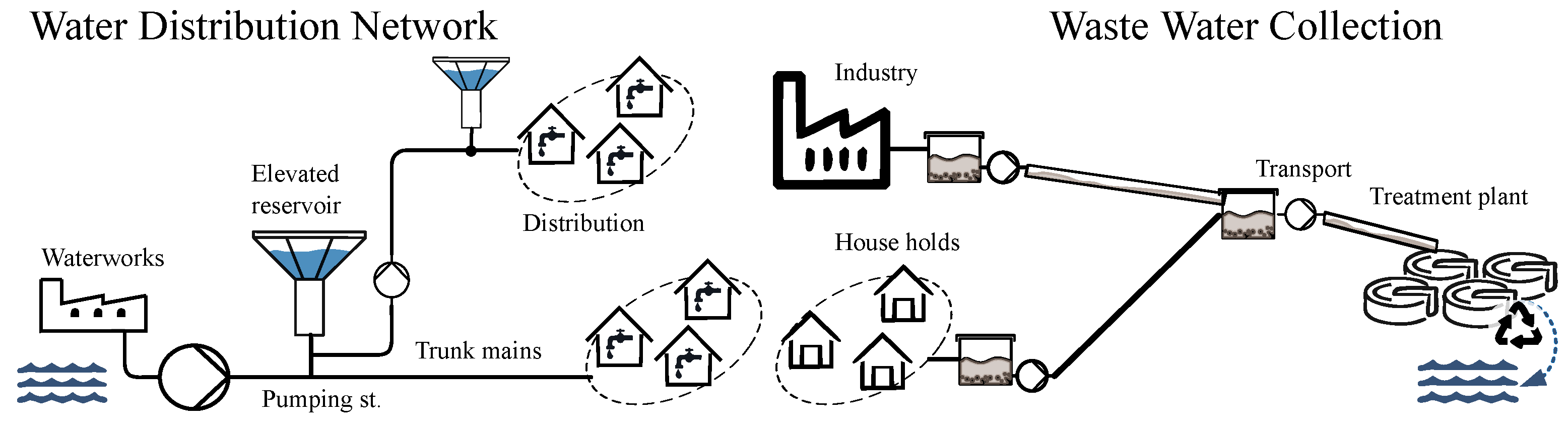
The laboratory focuses on emulating the qualitative physical effects of the water infrastructures. For this reason, network components such as pipes, valves, and pumps are scaled to mimic the properties of any water network. In the design of the laboratory the main features of the real large scale systems are considered, the two water infrastructures studied in this paper and some of its main components are illustrated in Figure 2.
Although these two networks differ in size, structure, and purpose, all of them are constructed of only a limited set of components. The networks can be divided into a few basic components and this division is used in the SWIL to create test-beds. Despite of their differences, these critical infrastructures have structural similarities. They are composed of a transmission part (trunk main, transport, sewer), several supply units (water towers, pumping stations), a distribution or collection zone and storage units.
Moreover, the emulated network can be easily extended by integrating additional elements, such as tanks, consumers, suppliers, therefore, covering a wider range of test scenarios with multiple producers or interconnected networks.
The features of each infrastructure are encapsulated into five types of modules (units): A brief system description is given for each unit with mathematical models representing each network’s main component.
2.1.1. Supply—Pumping Station/Storage
This unit has different functionalities: supply and storage. It consists of a set of pumps which boost the pressure in the pipe network. A model describing the pressure drop in a centrifugal pump is derived in [31]. Hence, the pump model is denoted by the polynomial
where is the flow through the pump k, > 0, and > 0 are constants describing the pump and is the rotational speed of the pump. Furthermore, the unit is equipped with a tank that can be used for water storage. The tank dynamics is given by the following differential equation
where is the cross sectional area of the elevated reservoir, h is the tank level and q is the inflow to the tank. When working as an elevated reservoir, the pressure at the elevated reservoir node is given by the algebraic relation,
where is a constant scaling the water level and pressure unit and z is the elevation of the tank inlet. The air pressure inside the tank is locally regulated such that it emulates a real geodesic level or tower elevation z.
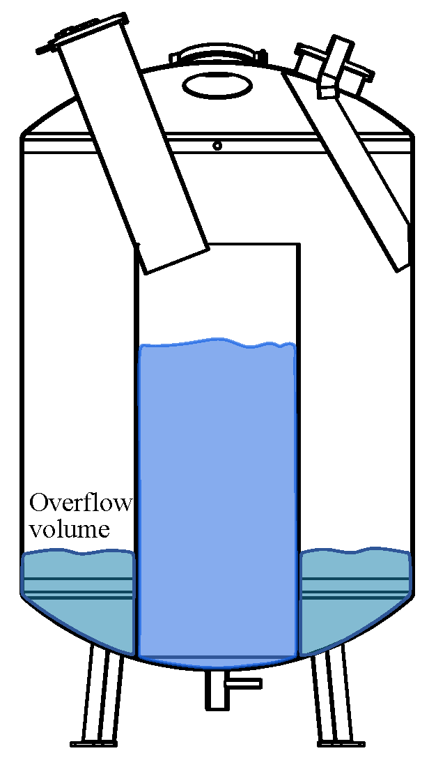
Moreover, this tank is equipped with an inner tank. The design of the tank is presented in Figure 3.
This feature allows using the tank as a retention tank/pond with a limited capacity and capture the overflow volume. The piping and instrumentation diagram of this unit is shown in the Appendix A—Figure A2.
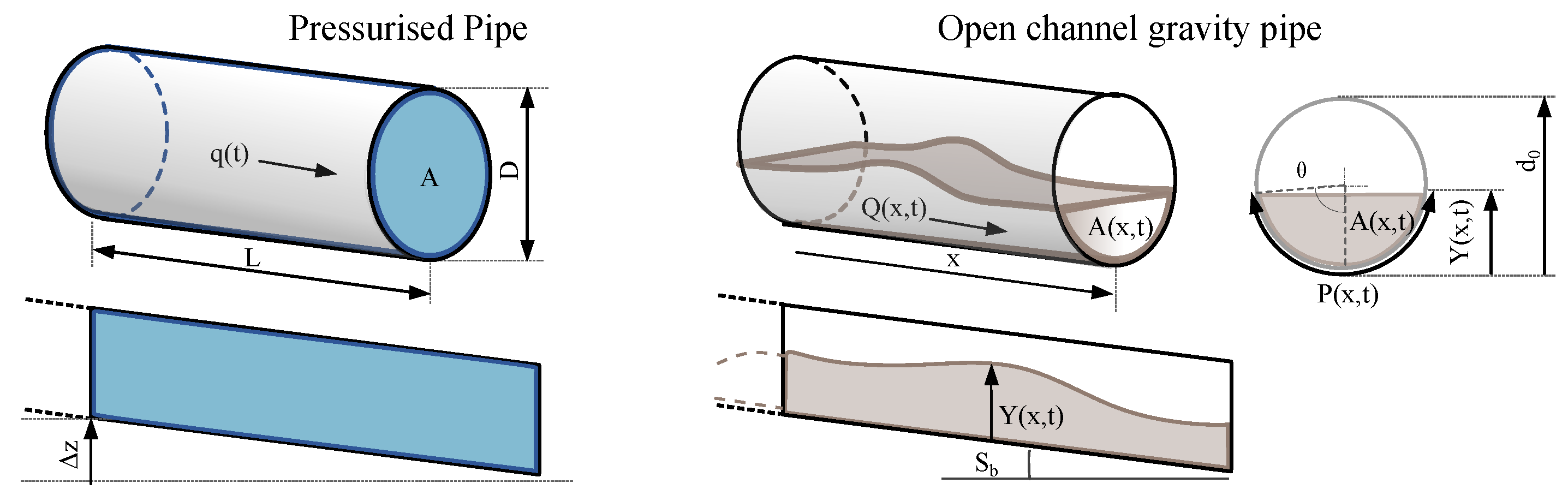
2.1.2. Transmission—Pressurised Pipe
In this laboratory, there are two types of units dedicated to the water transport, pressurised pipe unit and gravity sewer unit. This division is due to the different system dynamics that characterise the transport of water. In Figure 4 an illustration of the two types of pipes is shown.
The pipe unit emulates pressurised pipe lines in a network and it consists of a set of pipes of different diameter where several segments of pipes can be interconnected or bypassed in order to emulate different pipe length and configure the network topology.
In a water distribution network, surface roughness is not the only factor that produces resistance in the pipe during the operation; pipe bending, elbow, and fitting are also affecting the resistance. Form loss have the same structure as surface resistance, and when analysing long pipe lines as the ones modelled in this distribution network, form losses are considered negligible [32]. However, in the laboratory hydraulic circuit, the test-beds have a number of bends and elbows that is worth considering. In this model, the flow regime is assumed turbulent and the head pressure drop through the pipe element k caused is given by Darcy-Weisbach equation [32],
where is the head loss due to friction across the pipe element k, is the coefficient of surface resistance, is the coefficient of various form loss, L is the pipe length, D is the pipe diameter, q is the volumetric flow, g is the local acceleration due to the gravity. Then, the variation of the pipe resistance with respect to the quadratic flow through the pipe is given by [32].
The piping and instrumentation diagram of this unit is shown in the Appendix A—Figure A5.
2.1.3. Transmission—Gravity Sewer
This unit emulates the gravity sewers of a waste water collection. It consists of a set of pipelines that are dimensioned for open-channel flow and the slope of the pipes can be configured to cover several scenarios. The Saint-Venant equations are one of the most popular models to represent volumetric flow dynamics in open channel flow [33] where (6a) and represent the mass balance and (6b) is the momentum conservation, respectively:
where is the volumetric flow, is the water depth, is the cross section of the wetted area, is the wetted perimeter, the friction slope, is the bed slope and g is the gravitational acceleration—these variables are represented in Figure 4. This form of (6) is presented under the following hypotheses [34]:
- The flow is one-dimensional. The velocity is uniform over the cross-section and the water across the section is horizontal;
- The streamline curvature is small and vertical accelerations are negligible, hence the pressure is hydro-static;
- The average channel bed slope is small, therefore the cosine of the angle can be approximated to 1;
- The variation of channel width along x is small.
The algorithms that use these simplifications can be verified in the laboratory test-beds. For the design of the laboratory sewer, a steady flow solution of Saint-Venant equations is considered where is replaced by 0 and constant water depth along the channel [34]. Then, the volumetric flow Q and wetted area , the equations (6) are simplified to
For these operating conditions, the uniform flow in open channels can be described by the Manning’s equation [35].
where, for this work, the cross sectional area = , the wetted perimeter = , the hydraulic radius = A/, is constant coefficient corresponding to SI units, n is the Manning’s roughness coefficient and the bed slope is defined as .
The piping and instrumentation diagram of this unit is shown in the Appendix A—Figure A4.
2.1.4. City District—Consumer
This unit represents the end-users in a city district. The drinking water consumer consists of a valve that regulates the consumed water and a tank that collects it, the collected water is used as in-feed in the waste water system. Additionally, the geodesic level of the consumers can be emulated by introducing the equivalent air pressure in the tank.
In this project, controllable valves are used to represent the pressure drop generated at the end-users. Each valve varies its opening degree (OD) and it allows to control the pressure drop across it. The pressure drop due to the resistance factor is proportional to the quadratic term of the flow.
where is the conductivity of the valve k, q is the flow through the valve and is the pressure drop over the component. Valve manufacturers provide an accurate parameter for the controllable valve conductivity which depends on the opening degree of the valve and relates the flow and pressure drop as shown in [36].
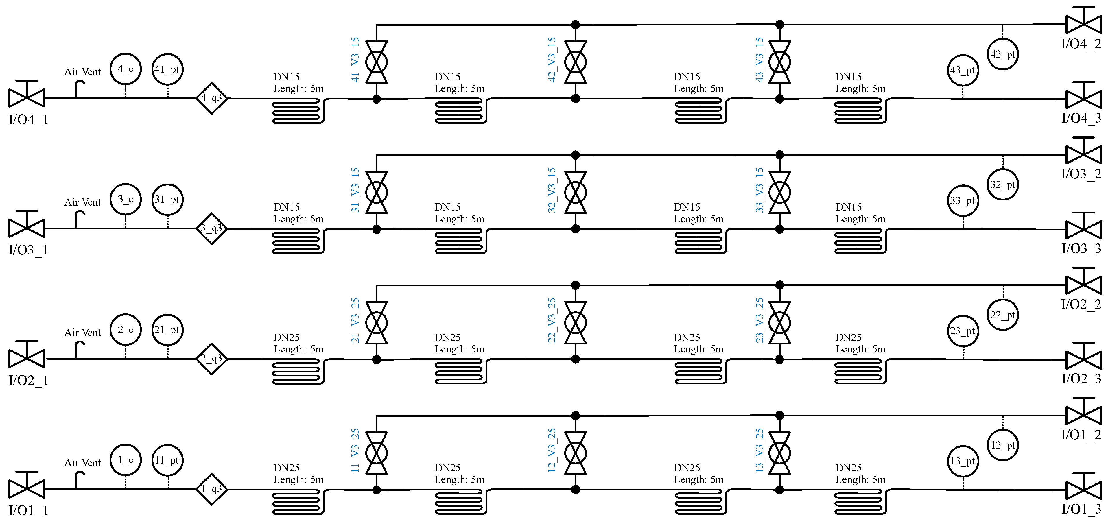
The piping and instrumentation diagram of this unit is shown in the Appendix A—Figure A3.
2.2. Network Design
The operation of the main components, or laboratory modules, in the water infrastructures must be also analysed as part of a network. When working with a small scale network, this analysis must consider the scaling effect, a list of the main factors considered for the scaling process is given in network scaling.
Then, simulations of the scaled down networks are developed based on the mathematical models presented in the previous subsections [37]. The objective of these simulations is to design the correct size of the module components and evaluate the capacity of the modules when they are interconnected through a pipe network. Furthermore, having a simulation environment of the test-bed can support the preparation of the laboratory modules for a given study case. For example, by choosing certain topology, pipe length or magnitude of the signals input and disturbance signals.
2.2.1. Network Scaling
In order to transform a large-scale water infrastructure into a laboratory test-bed, this project has performed some simplifications to reduce the network size. This size reduction is based on four factors:
- Number of nodes: The end-users that are geographically close are aggregated and they are considered as a single consumer [38]. This node reduction does not affect the overall network structure;
- Number of pipe types: A real pipe network contains a large amount of pipe types which differ in size and material. In order to adapt the pipelines to a laboratory module, the piping is designed with a limited number of pipe diameters and lengths. The pipe networks at the laboratory are built with two pipe diameters for pressurised pipes (mains and branches), and one pipe diameter for gravity pipes (sewer pipes);
- Dimensionality: The magnitude of the network pressures and flows are reduced to meet the test-bed component requirements (sensors and actuators range). For instance, to get an idea of reduction in the magnitude, in the case of Bjerrinbro (a small water utility) the maximum supply pressure is approximately reduced from 5 bar to 4 m and the maximum supply flow from 80 to 0.4 ;
- Time scale: The scaled-down test-beds allow accelerated tests. A test that would last several days in real-life can be replicated at the laboratory in hours. The tank modules have fixed dimensions, but its dynamics can be adjusted by varying the time scale of the tests.
All real networks differ in size and characteristics, and, therefore, the abstraction that transforms any full-scale water infrastructure into a test-bed introduces an error. In order to meet the laboratory physical limitations, an approximation of the network characteristics is required.
When choosing a smaller size for the modules, the focus of the design is to emulate most of the qualitative properties of a real network, such as pipe network topology, geodesic levels, flow regimes (turbulent and open-channel flow), system delays, actuation, and disturbance dynamics. For this reason, this study assumes that some errors introduced by the scaling, such as exact scale friction loss in the pipe network or pressure and flow ratio, have a minor impact on the tests of control solutions, since the verification method that this paper proposes relies on a proof of concept validation. The scalability of the solution is not addressed here.
2.2.2. Water Distribution Network Design
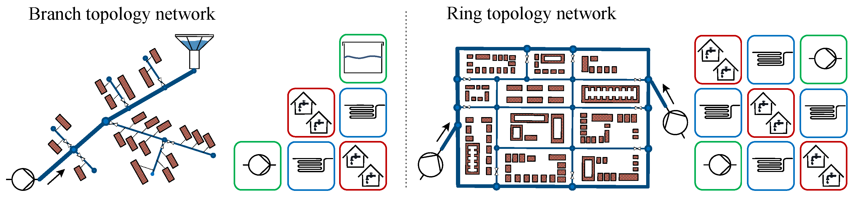
There are multiple elements that characterise a pipe network structure, such as ground levels, pipe size, or topology [32]. Two of the most representative topologies branched and looped geometry (ring) are illustrated in Figure 5. Next to each topology, examples of equivalent networks constructed with laboratory modules are shown.
It can be observed that by changing the position of few modules, the structure and management of the network are significantly changed. The test-bed in Figure 5 is transformed from being a branched structure with a single pumping station and elevated reservoir to a ring topology with two pumping stations and an increased number of end-users.
The ground levels of each urban district can be emulated by using the pressurised tank systems at the consumer and pumping modules.
Simulation
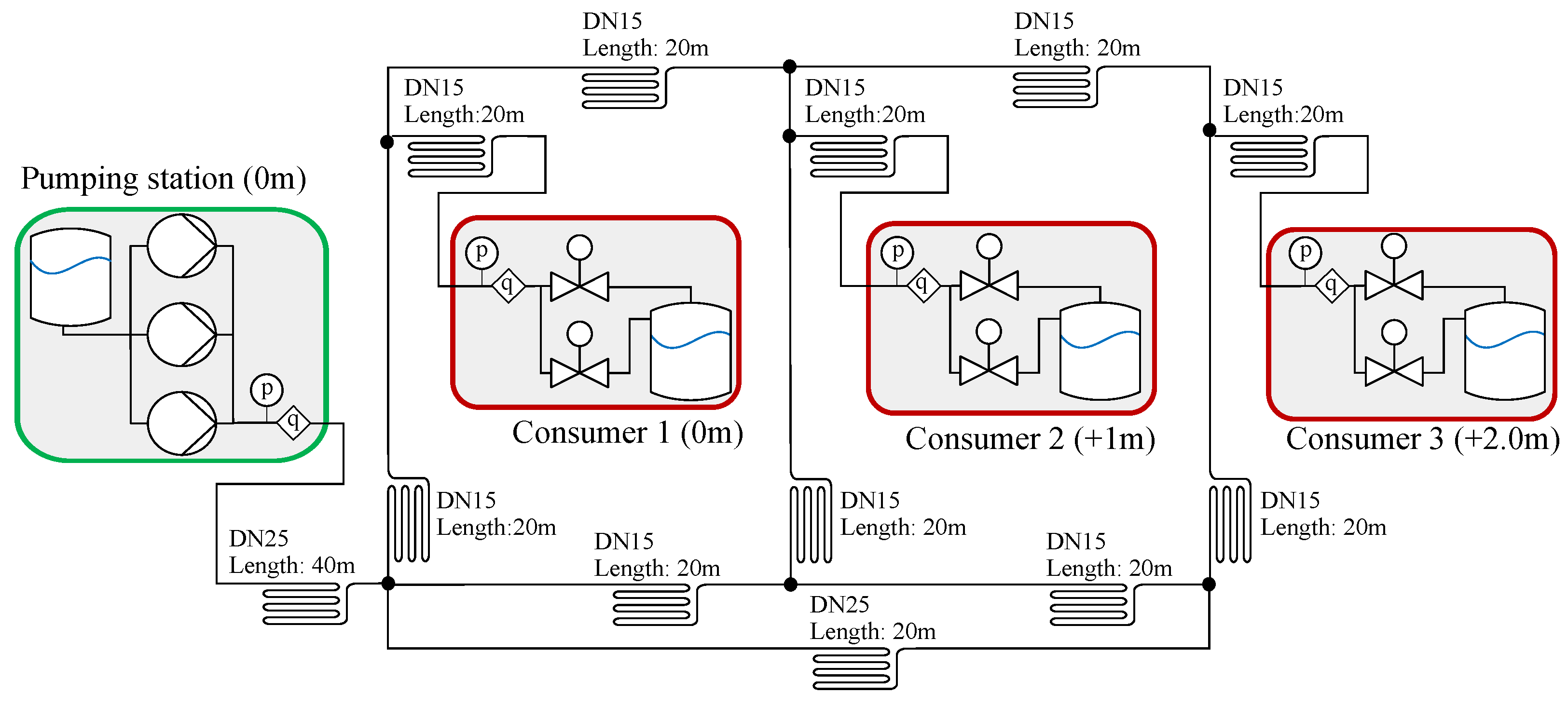
A simulation of a WDN is built with the purpose of determining a reduced pipe size and the maximum capacity of the test-beds. The network structure used for this simulation is a standard WDN with an arbitrary ring topology network that connects a pumping station (green block) and six end-users (red blocks), see Figure 6. This network structure is inspired by the network examples studied in [32]. The capacity of this network is restricted by the pumping station, the number of consumers and pipe size. The pumping station and consumer operation is fixed and the length and diameter of the pipe units, mains and branches, are adjusted accordingly to fulfil the following conditions:
- The flow regime is turbulent in all the network pipes. Then, the friction losses are calculated with the model developed in (5);
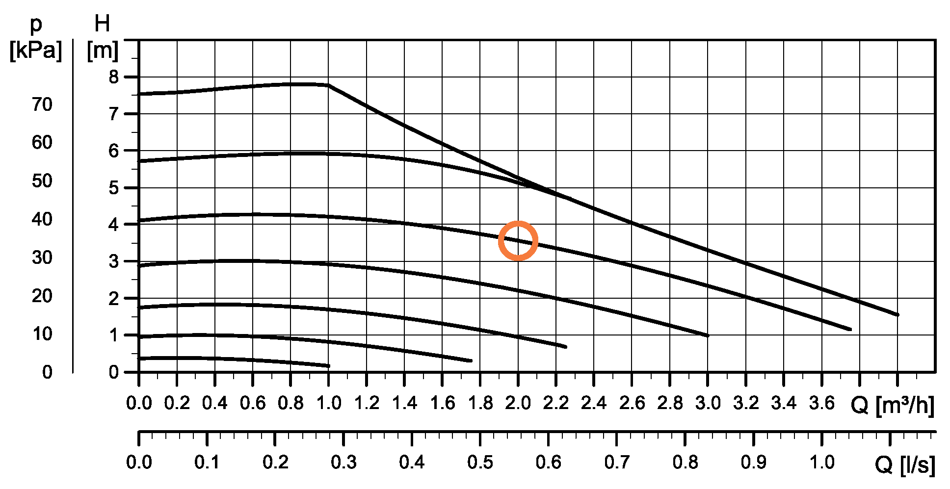
- The total head is supplied by a set of Grundfos-UPM3 pumps, its nominal operation is around q = 2 and = 0.4 bar with speed = 80% for each pump, see curve in Figure 7;
- A fraction of the total head loss (1/3) corresponds to friction loss (pipe), and the other fraction (2/3) corresponds to the pressure drop at the end-users (valves).
As mentioned on Section 2.2.1, a generalisation of the structure and sizing of a pipe network implies the introduction of some error since the ratio between these fractions varies from network to network. The simulations of the reference network models are developed in modelica—Dymola. Remark that the simulation package is built with a modular structure such that the network topology can be easily modified.
2.2.3. Waste Water Collection Design
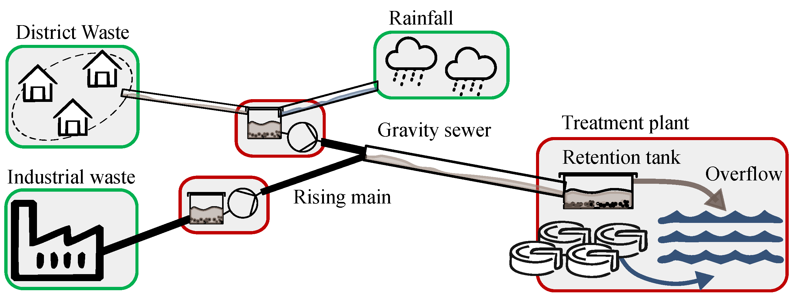
The sanitary sewers are large networks of underground pipes that collect domestic sewage, industrial waste water, and rain-fall. This study focuses on a combined scheme to represent the characteristics of a typical sewer network in the laboratory, Figure 8 illustrates the main elements in a combined sewer. In this model, the waste water conveys from different sources to the same pipe in order to be transported to retention tanks and a centralised treatment plant. The transport typically requires of a combination of both gravity sewers and pressurised pipes to overcome the elevations of the terrain. Additionally, several control elements such as retention tanks are introduced in critical locations along the network to regulate the discharge. Finally, a treatment plant receives all the water and rejects water when exceeds its capacity (overflow).
A WWC constructed with laboratory modules must comprise of the equivalent elements: water sources (green blocks) and storage elements representing retention tanks and treatment plant (red blocks). The laboratory blocks are interconnected with pressurised pipes (rising mains) or gravity sewers according to the application requirements.
Simulation
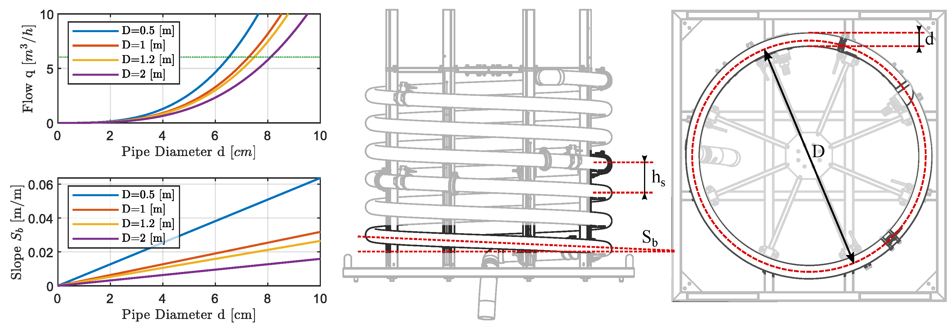
In the design of the sewer pipe module, some of the standards for sanitary sewers presented in [39] are considered. The dimensions of the sewer unit are represented in the mechanical drawing shown in the Figure 9 (right), and the values of these parameters are calculated by solving the Manning’s formula (8) with the following conditions:
- The maximum flow through the pipe given from the the nominal flow of a pumping station (3 pumps with 2 each);
- The water covers half of the pipe () for a nominal volumetric flow;
- In this unit the bed slope is constrained to the physical limitations of the laboratory unit. Due to the coiled shape of the conduct, the minimum height difference for each loop is the diameter of the pipe.
The simulation results are shown in Figure 9 (left). The pipe diameter d is of 8 cm (DN80) and a coil diameter D of 1 m are selected according to the given requirements. For a total pipe length L of 19.6 m, the estimated nominal delay = 29 s.
2.3. Hardware Design
This section describes the structure of the laboratory for control and real-time monitoring. First, a description of the data acquisition (DAQ) system and control structure is presented. Second, the communication architecture implemented is presented. Both systems are designed to emulate the control and monitoring hardware of a real water infrastructure.
2.3.1. Data Acquisition
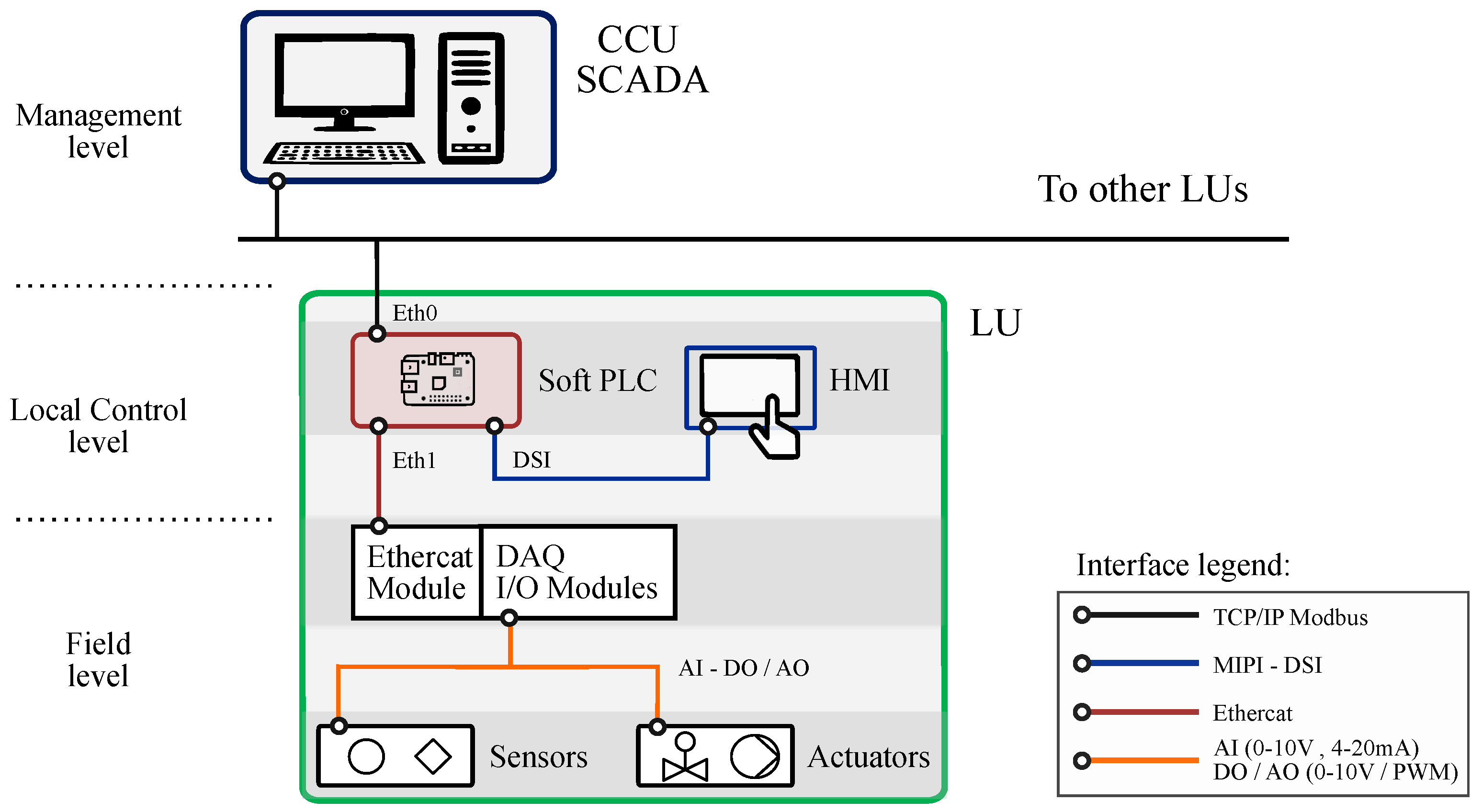
The scheme in Figure 10 shows the laboratory DAQ and control architecture that is divided into three levels:
At the management level, the central control unit (CCU)—SCADA gathers, processes, and monitors real-time data from the local units (LU).
At the local control level, the soft-PLCs perform three functions: data acquisition from the Beckhoff I/O Modules via Ethercat, communication with the CCU or other LUs and the control and safety of the LU. The soft-PLC consists of a Codesys runtime control installed on a Raspberry Pi (RPI) [40]. Moreover, the RPI is equipped with an HMI which provides a graphical interface for local monitoring, configuration, or manual control.
At the field level the I/O modules are connected to the sensors and actuators with different signals. The laboratory modules are provided with sensors to measure pressure, flow, temperature, conductivity, level. The complete list of the instrumentation equipment for each unit is shown in the Appendix A.
2.3.2. Communication Network
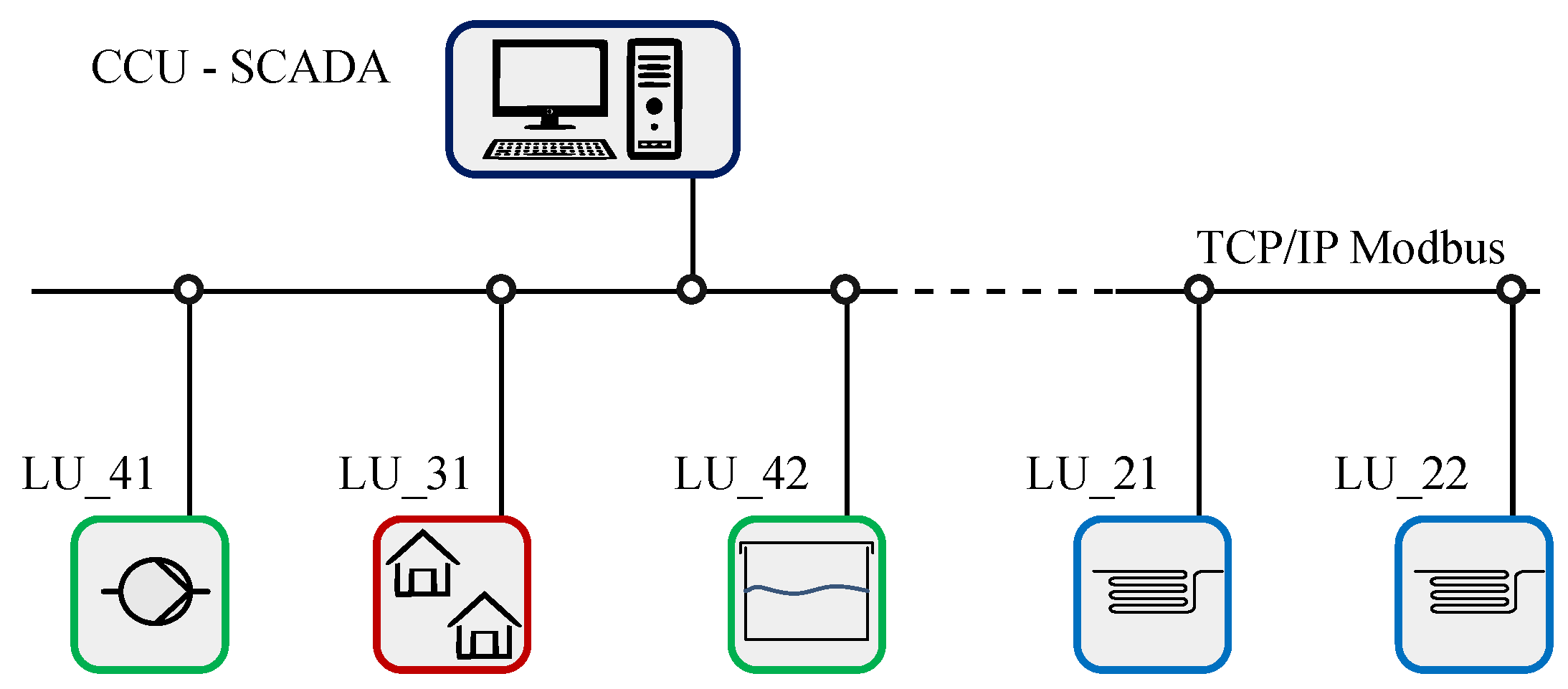
The communication architecture of the laboratory elements CCU and LUs is designed such that it can adapt to two control architectures: centralised or distributed control. Therefore, the communication interface is a modular system developed with MODBUS TCP-IP. Nevertheless, the hardware and software of the laboratory can also implement other communication protocols such OPC-UA.
The Figure 11 illustrates the modular communication architecture where the LUs are interconnected to a LAN together with a CCU that can be used for centralised management of the modules. The CCU is interfaced with Simulink for monitoring and fast implementation of the supervisory control algorithms. An alternative interface method is developed in Python when the studied management requires distributed communication between LUs.
2.3.3. Safety and Local Control
During the design of the LUs, a risk assessment is performed with the purpose of avoiding failures and providing a secure operation of the laboratory. In order to guarantee a fail-safe operation, two protection layers are implemented on the laboratory equipment, hardware, and software safety controllers:
The first layer consists of safety valves that are installed at critical points of the laboratory such as boilers or pressurised tanks. These elements limit the maximum operating temperature and pressure, respectively. Additionally, hardware safety switches turn-off the power supply when the operation is not safe laboratory.
The second layer consists of software safety controllers that are implemented at the soft-PLC. They regulate the minimum and maximum tank level, avoiding air in the hydraulic circuit or water overflow.
3. Results
In this section, four case studies with laboratory experiments are presented. These experiments aim to reproduce different scenarios affecting the management of a real utility and illustrate the versatility of the SWIL.
First, the steps to transform real utility problems into laboratory experiments are explained. Then, a description of the laboratory experiments for each study case is given. This includes an introduction to the research contribution and a description of the laboratory customisation for each study case.
3.1. Test-Bed Configuration
First, information from the network structure is used to identify the main features of the studied infrastructure. The main components of the network, such as pumping stations, demand nodes, and rain collection or storage units, are replaced by their equivalent laboratory module and interconnected with pipe modules, emulating the real network topology. The pipe length, ground elevation and sewer’s slope can be adjusted to meet the study requirements while considering the laboratory restrictions, recall scaling considerations in Section 2.2.1.
The laboratory test-beds are equipped with multiple sensors and actuators, this means that in most studies there is redundancy of the measurements. With a vast number of sensors it is possible to choose a subset that matches the configuration of a real system. These experiments restrict the use of the sensors according to the characteristics (number and relative position) of the studied network.
Then, real datasets of the network operation, such as water consumption, rain-events, or industrial discharge are used to adapt the test to the given problem. Note that, the laboratory experiments are performed in a smaller scale, this means that the magnitude of the real signals and time scale are adapted to meet the operation range of the test-bed.
3.2. Study Cases for Water Distribution Networks
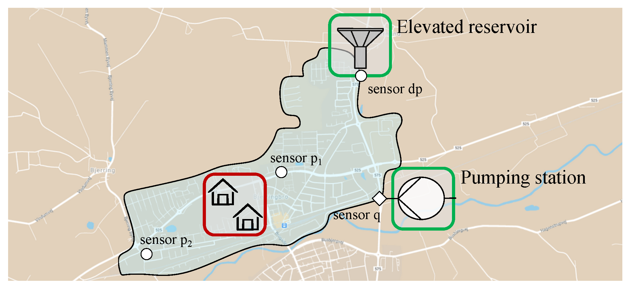
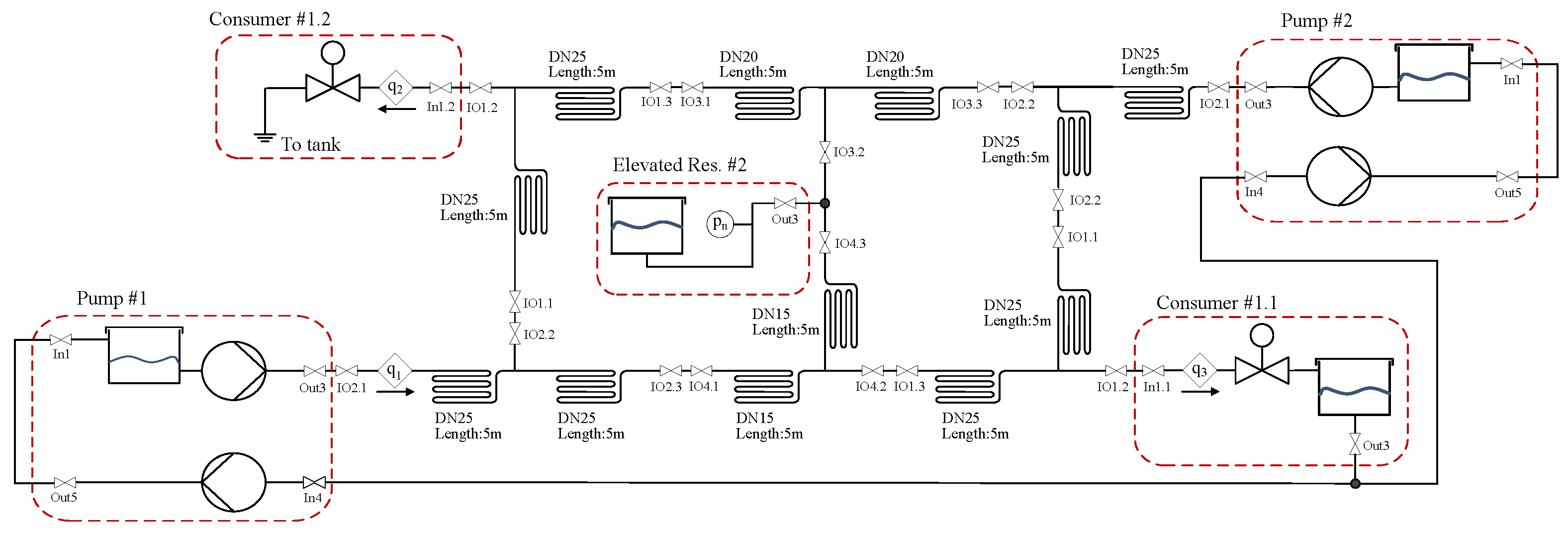
This study case is inspired by the WDN at Bjerringbro, a small city district in Denmark, see Figure 12. This water utility has one pumping station, one elevated reservoir and multiple end-users distributed along a pipe network. The main elements of Bjerringbro’s network are identified (ring topology, number of pumping stations, elevated reservoirs, consumers, and sensors), and an equivalent scaled-down network is emulated with the laboratory modules as Figure 13 shows.
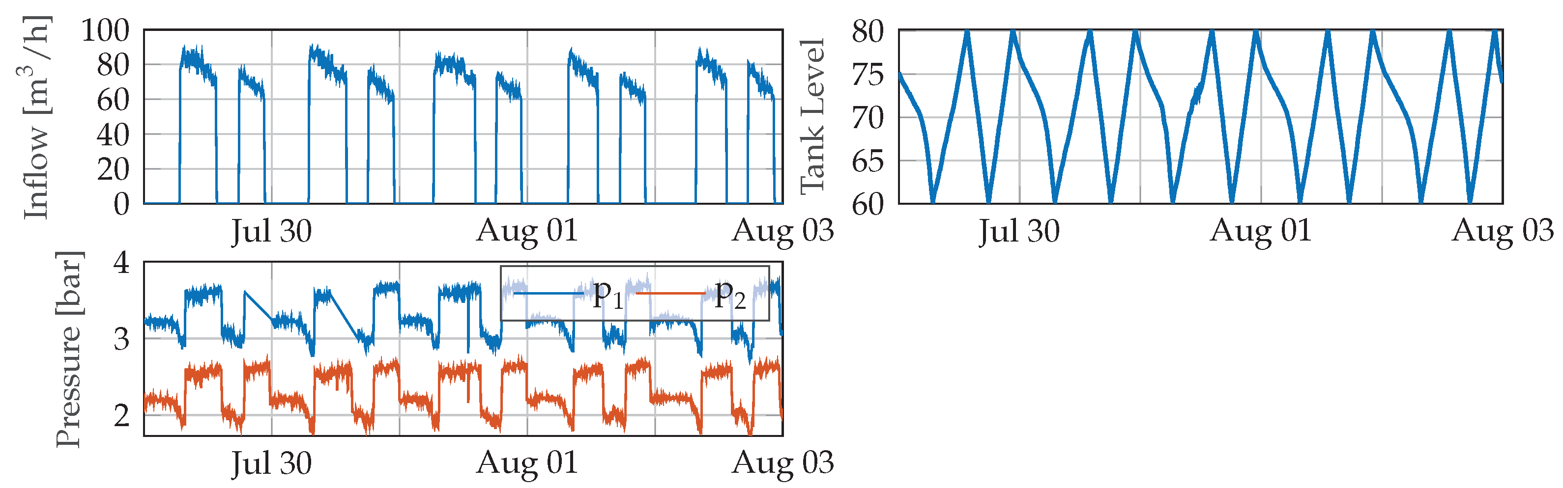
A graph with real data from this district is presented in Figure 14 as a reference of the water distribution network operation. This utility operates with an ON/OFF controller that regulates the elevated reservoir level.
Note that, the laboratory test-bed is equipped with an additional pumping station which is not existing in the real network, this component is added with the objective of evaluating the network management with two supply nodes.
3.2.1. Optimal Management with Multiple Supplies in Bjerringbro
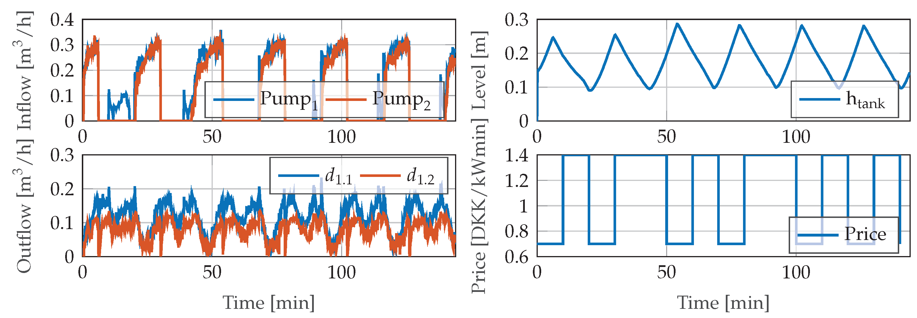
This study case summarises the work presented in [41]. This study uses a network structure with two pumping stations and an elevated reservoir. This project proposes a distributed network management where a non-linear model predictive control (MPC) acts as supervisory control and PI controllers locally regulate the flow at the pumping stations. The supervisory control controls the tank level (h) by regulating the inflows (Pump and Pump), this controller is designed to minimise the operation cost and pressure variations at the end-users. The operational cost is evaluated using the power consumption of the pumping stations and the energy price. The district demands ( and ) are emulated with real profile, and in the control, they are estimated using a Kalman filter. The control strategy is validated at the SWIL with the test-bed represented in Figure 13. The experimental results in Figure 15 show that the supervisory control schedules the pump actuation for the time-periods where the energy price is low, the study shows a reduction in the operational cost and pressure variations with respect to a standard ON/OFF tank filling that utilities typically operate with.
3.2.2. Optimal Management with Unknown Network Model in Bjerringbro
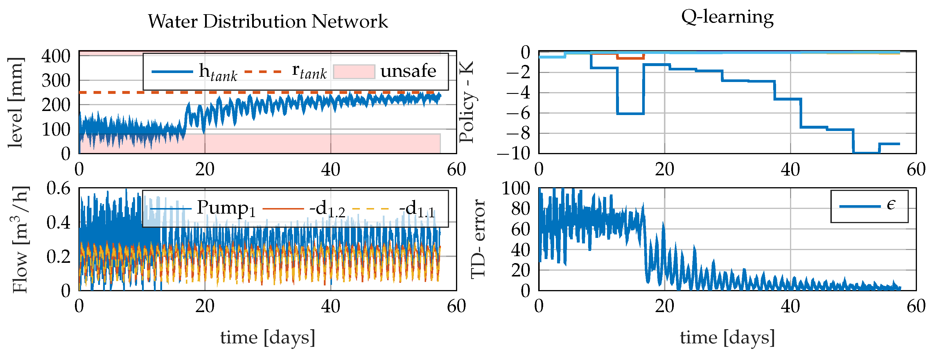
This study case summarises the work presented in [42], the objective of this experiment is to design an optimal controller without the knowledge of the system dynamics, in this case the network structure consists of a single pumping station. The network management is based on a reinforcement learning (RL) algorithm which finds the supervisory system policy based on a cost function criteria that minimises high control actions and energy consumption. The results of this work are shown in Figure 16. The total end-user’s demand ( and ) is learned using a Fourier series basis. Additionally, the safety of the operation is guaranteed during the learning period with a policy supervisor.
This methodology is an AI control approach without stability proof, but it learns a satisfactory network management despite not having an extensive knowledge of the network, since the only information is the measured data. The safety boundaries are not violated and the end-user’s water supply is guaranteed during the operation of the network. The laboratory experiment gives evidence of the robustness of the method, enabling the further investigation of AI techniques for control of real systems.
3.3. Study Cases for Waste Water Collection
3.3.1. Optimal Management of a Treatment Plant with Inlet Flow Variations in Fredericia
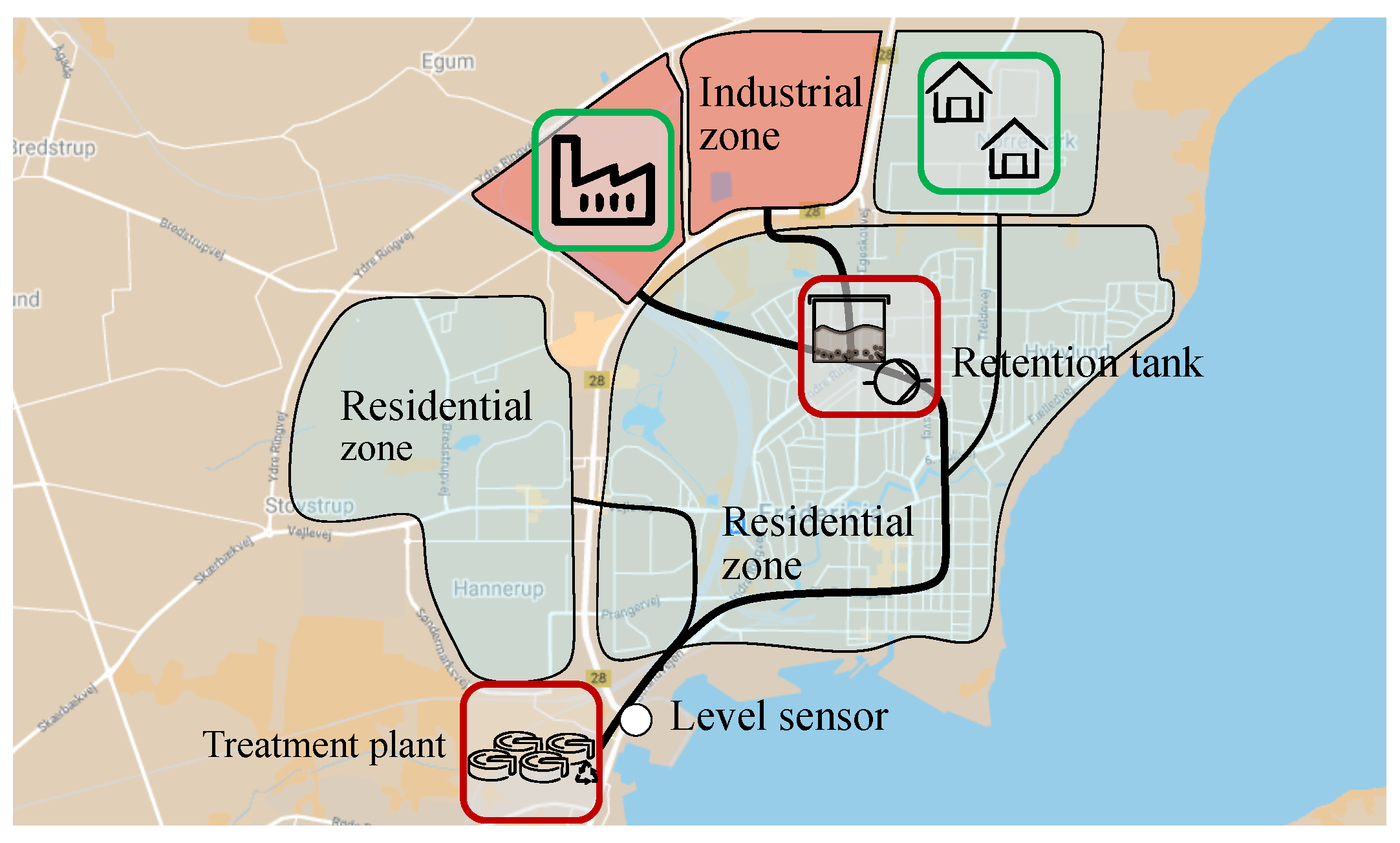
This study case summarises the work presented in [43], in this work the management of the waste water collection in Fredericia (Denmark) is studied. In this city, several industrial zones (red area), residential zones (blue area) and precipitations discharge waste water to a collection network that conveys to a treatment plant, see Figure 17.
The treatment plant operation is based on a chemical process that increases the performance when the working conditions are stable. The waste water discharges from industry are stochastic disturbances that have a big impact on the treatment plant’s performance. Therefore, the network management must regulate the inlet flow and pollutant concentration such that their variations are minimised at the treatment plant.
This work aims to minimise the inlet flow variation by controlling the industrial discharge, For this reason, the potential installation of a retention tank that regulates the varying discharge using MPC is studied. The controller considers an estimation of the household discharge via Kalman filter and takes into account the transport delay of the sewer network.
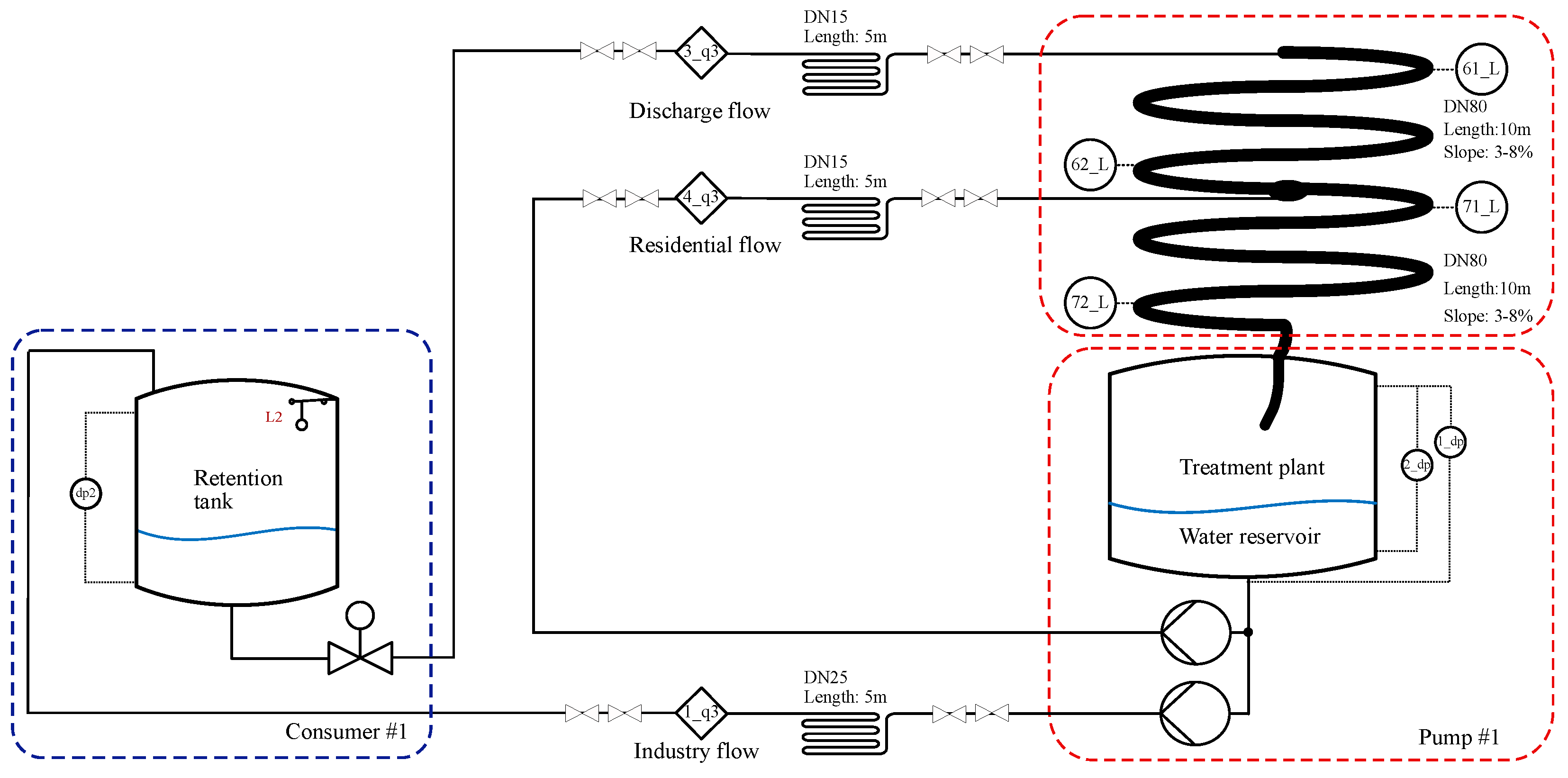
This scenario is reproduced in test-bed where the main components of the network are represented (main waste water sources, retention tank, and sewer scheme), see Figure 18. The industry and residential discharge is locally controlled to reproduce the pattern extracted from real-data. Additionally, the only real-time measurement available is the sewer level at the inlet of the treatment plant, the controller in the experiments uses only one level sensor () to estimate the inlet flow.
The graph in Figure 19 shows a clear minimisation of the flow variations with respect to the non-controlled operation. The experimental results show that the installation of a new control element in the network is feasible since it can considerably improve the operation of a real network.
3.3.2. Fault Tolerant Control of a Sewer Network with the Backwater Effect in IshøJ
This study case is summarises the work presented in [44]. In this work a section of the waste water collection system in Ishøj (Denmark) is analysed, see Figure 20.
The structure of this section consists of a gravity sewer and two open basins used as retention tanks for rain drainage, one on the upstream and the other on the downstream. The knowledge of the tanks storing the volumes and the flow are needed to develop both a controller that optimises the system operation and a model which predicts overflows. This study proposes a data-driven model which accurately fits the network features, in particular, the back-water effect.
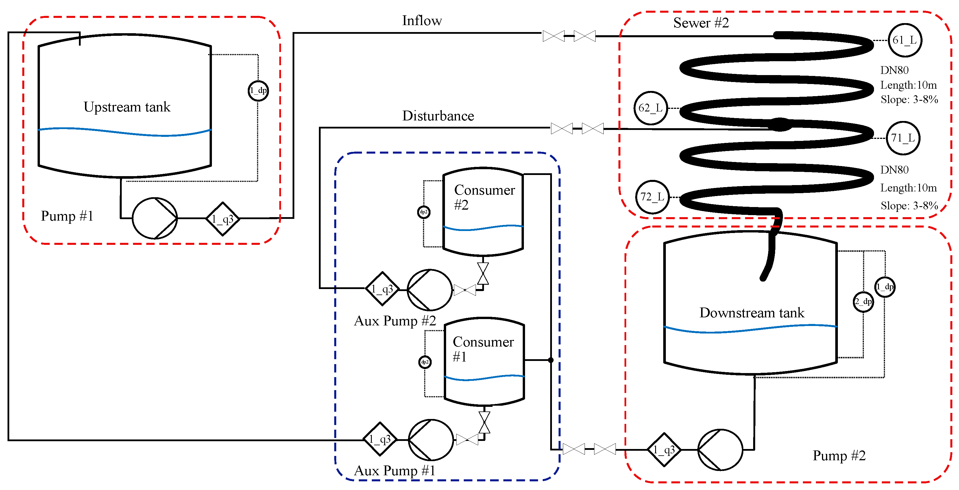
A test-bed with equivalent network features to the Ishøj’s network section is emulated at the SWIL, the diagram of the test-bed is represented in Figure 21. Although Ishøj´s scheme is a separate rain drainage collection, this laboratory experiments use disturbance profiles of combined household waste water and rainfall. The open basins are emulated with tanks placed at the upstream and downstream, the network disturbances are emulated by auxiliary modules equipped with a reservoir tank and a pump.
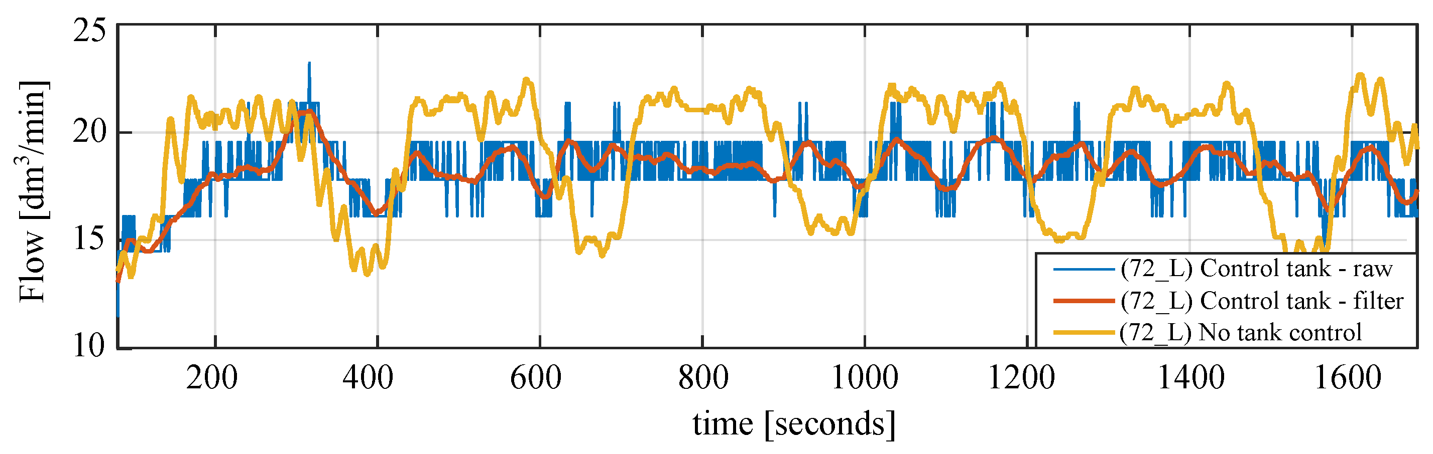
The results in Figure 22 show a comparison between two model structures, kinematic wave (KW) and diffusion wave (DW). The level measurements are taken at different points of the sewer pipe, for simplicity, this paper only shows the measurements at the sensor (62_L) where the backwater effect is observed.
The effectiveness of the proposed models is presented, showing the capacity of each method for capturing back-flow inside the pipes. The experimental results show that the understanding of the back-water phenomena with a data-driven model can help the future development of fault tolerant controllers which consider this effect.
4. Discussion
This paper presents the development of a test facility for monitoring and real-time control of urban water networks, as well as several case studies where the laboratory contributed to the understanding and verification of the new control solutions.
The authors of this study consider that the test-beds configured at the SWIL meet the design criteria and the results support the design hypotheses: The facility at Aalborg University is able to emulate three kinds of water infrastructures. The modular properties of the test-beds allow to adapt the main features from different real networks, including datasets from the water utilities, thus increasing the realism of the laboratory test. Furthermore, the authors consider that replicating and testing certain management situations, that cannot be repeated in real infrastructures, can contribute to advance in the monitoring and real-time control of urban water networks. The verification of control methods in a customised test-bed allows quick prototyping or realisation of “proof of concepts”.
On the scientific side, the four study cases analysed at the SWIL show that this facility enables the research of water infrastructures management in a novel and unique manner. The multiple configurations of the test-beds create a suitable environment to validate new control solutions on a specific real problem. The results show that the data collected on the emulated networks at the laboratory is qualitatively comparable to the real infrastructure, see Figure 14 and Figure 15.
This laboratory allows to test the reliability of a newly developed technology and study its limitations with no consequences in case of failure. This type of validation is not feasible to perform in real infrastructures in which the impact of having a management failure can cause severe consequences such as environmental damages or damages of the infrastructure equipment, such as pumps or pipes, and discomfort of the end-users. For instance, in this safe environment, model-based controllers like MPC can be tested against model uncertainty, the propagation of pollutants in the network can be studied and develop methods to contain them, learning-based controllers can freely search for the equilibrium between optimal operation and resilient operation or network operators can evaluate the feasibility of a real network upgrade by connecting to the network additional retention tanks or pumping stations. Thus, the laboratory validation constitutes a safe and inexpensive method since the resources required to perform a test at the SWIL are relatively low: The preparation of the test-beds only requires of the assistance of a laboratory technician, and the energy and water usage can be considered negligible during the test.
Data-driven control solutions can particularly benefit from the laboratory environment. The data collected during the laboratory experiments can support the study of certain physical phenomena like water leakages and back-water or train self-learning control algorithms.
Moreover, although fault-detection methods are not addressed in this paper, these methods can also be validated in the laboratory by recreating water leakage scenarios or water contamination propagation without water being wasted. This safe testing provides a sustainable manner of discovering new technology. The laboratory is equipped to study contamination, it uses conductivity sensors measuring salt concentration as a proxy to contamination sensors and a reverse osmosis unit to purify water.
Although the presented experiments satisfactorily reproduce the qualitative physical effects and the monitoring and management of a real water infrastructure, having scaled-down networks reduce the degree of realism. This means that the dimensionality of the tests is bounded by the number of modules available and the laboratory space, actuators are not ideally scaled-down and might introduce unwanted effects in the experiments and small networks can cause coupling between network elements.
In this work, the management scenarios are studied for each infrastructure individually. However, the infrastructure interconnection can and should also be studied. Various networks—water, heat, electricity—are no longer independent. Tons of water are used during electricity production. Vice-versa, electricity is needed for water distribution and heat production. This laboratory facility allows the study of different water networks and their interconnections, as well as links to the power supply and the internet. Research fields related with cyber-security and critical infrastructures can also be studied in this facility. The laboratory modules are already equipped with power meters at pumping and heating stations to study these problems.
5. Conclusions
The development of the smart water infrastructures laboratory has been presented. Here, the design process followed to reproduce a scaled-down water network with different modules is summarised. The main elements and features of the water infrastructures are represented in the laboratory modules. The configuration of these basic components such as pumps, tanks, or network topology are elements which characterise a network. Calculations based on component models are performed to adjust the sizing of the components to the water network properties, laboratory requirements and restrictions. The implemented DAQ system and communication interface recreate a real communication network with local smart-meters and controllers interconnected with a SCADA. This system has a modular architecture that facilitates the expansion of the test-bed and the integration of new technology or management solutions.
The aforementioned case studies are examples of the many possible configurations of the laboratory, where the SWIL demonstrates the capacity to replicate real problems in laboratory test-beds and reproduce real management scenarios in a scaled-down network.
Author Contributions
All authors have contributed equally to this manuscript, all the authors have read and agreed to the published version of the manuscript. All authors have read and agreed to the published version of the manuscript.
Funding
This research was funded by Poul Due Jensen Foundation (Grundfos Foundation).
Institutional Review Board Statement
Not applicable.
Informed Consent Statement
Not applicable.
Data Availability Statement
The datasets supporting the laboratory studies have been provided by different local water utilities in Denmark: Bjerringbro vandforsyning, Fredericia vandforsyning and Ishøj Forsyning.
Acknowledgments
Financial support from Poul Due Jensen Foundation (Grundfos Foundation) for this research is gratefully acknowledged. Water utilities for sharing the network datasets. The Codesys Group [40] contributed to the project by providing software licenses to part of the laboratory equipment. We are also grateful to Saruch Satishkumar Rathore, Kirsten Mølgaard, Krisztian Mark Balla for sharing their experimental results and Tom Nørgaard Jensen for his input and advice during the design process of the laboratory modules. Finally, we would like to express our gratitude to the water utilities, Bjerringbro vandforsyning, Fredericia vandforsyning and Ishøj Forsyning for providing the network data.
Conflicts of Interest
The authors declare no conflict of interest.
Abbreviations
The following abbreviations are used in this manuscript:
| MDPI | Multidisciplinary Digital Publishing Institute |
| SWIL | Smart Water Infrastructure Laboratory |
| AAU | Aalborg University |
| WDN | Water Distribution Network |
| WWC | Waste Water Collection |
| MPC | Model Predictive Control |
| RL | Reinforcement Learning |
| RPI | Raspberry Pi |
| CCU | Central Control Unit |
| LU | Local Unit |
| LAN | Local Area Network |
| HMI | Human-Machine Interface |
| SCADA | Supervisory Control and Data Acquisition |
| DAQ | Data Acquisition |
| I/O | Input /Output |
| OPC UA | Open Platform Communication Unified Architecture |
| PLC | Programmable Logic Controller |
| PWM | Pulse Width Modulation |
| KM | Kinematic Model |
| DM | Diffusion Model |
Appendix A
This appendix shows the piping and instrumentation diagrams for each of the laboratory units with a complete list of installed components.

Table A1.
List of sensors and actuators installed on the laboratory units.
| Tag | Type | Model |
|---|---|---|
| Sensor: Level | Microsonic ZWS-15/CU/QS | |
| Sensor: Conductivity | GF - Type 159001730 | |
| Sensor: Pressure and temperature | Grundfos Direct Sensor RPI+T 0-1.6 | |
| Sensor: Differential pressure | JUMO 404382 | |
| Sensor: Pressure | JUMO 404327 | |
| Sensor: Volumetric flow | Festo SFAW-32 | |
| Sensor: Volumetric flow | Festo SFAW-100 | |
| Sensor: Volumetric flow | Endress+Hauser Proline Promag 10 | |
| Actuator: Valve DN 15 | Belimo LQR24A-SR+R2015-1-S1 | |
| Actuator: Valve DN 25 | Bürkert 8804 | |
| Actuator: Valve | Danfoss EV210B+BE024DS | |
| Actuator: Pump | Grundfos UPM3 25-75-130 | |
| Actuator: Air Control | Festo: VPPE |
Figure A1.
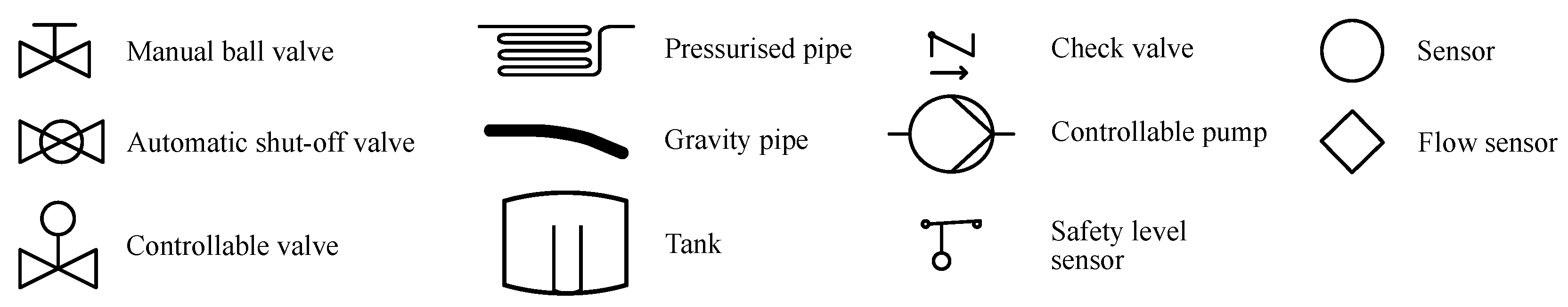
Legend of the piping and instrumentation diagrams.

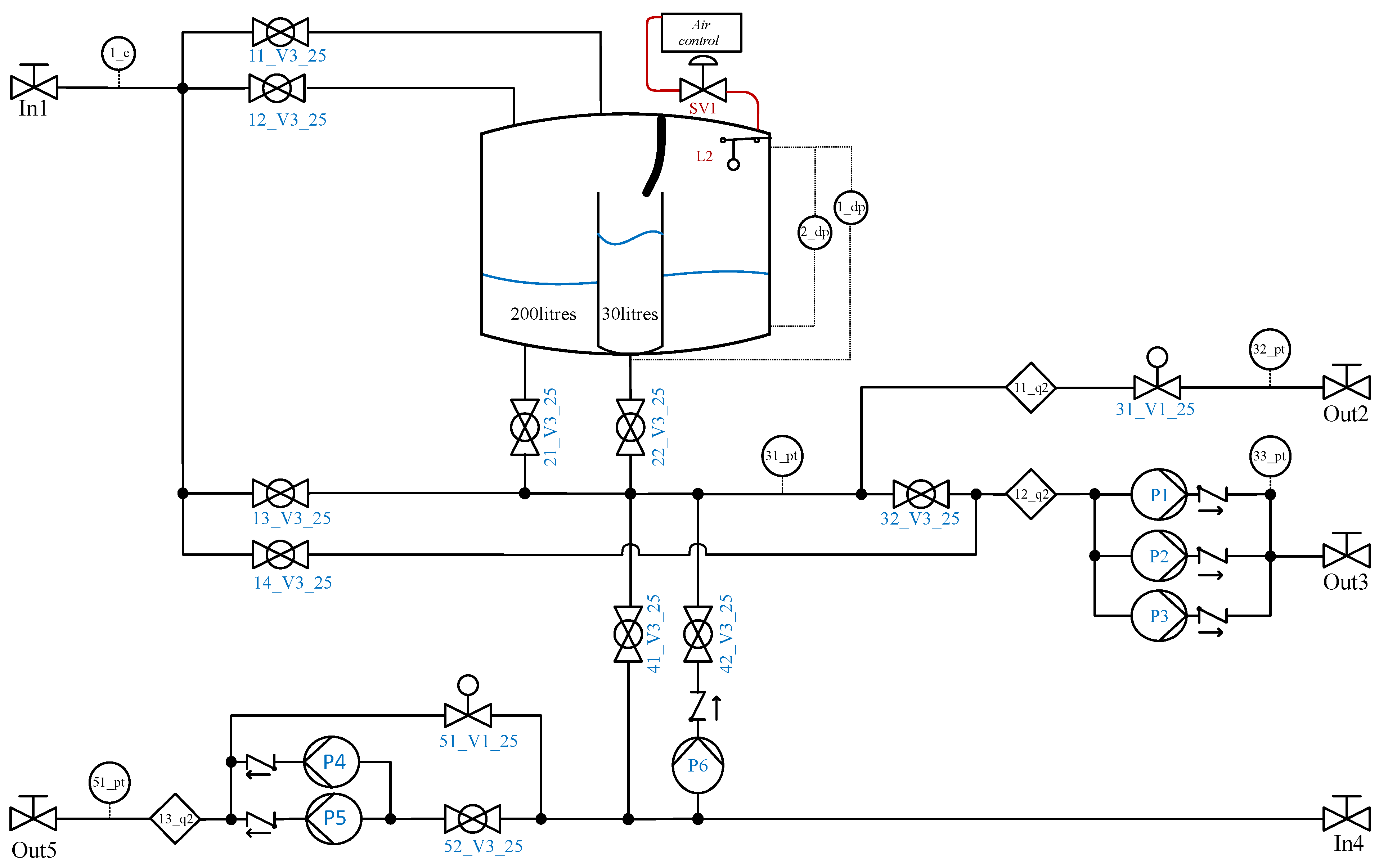
Figure A2.
Piping and instrumentation diagram of the pumping station unit. The legend is shown in Figure A1 and the details for each component are listed in Table A1. Shut-off valves are locally controlled to block or bypass different hydraulic circuits, thus enabling different features.

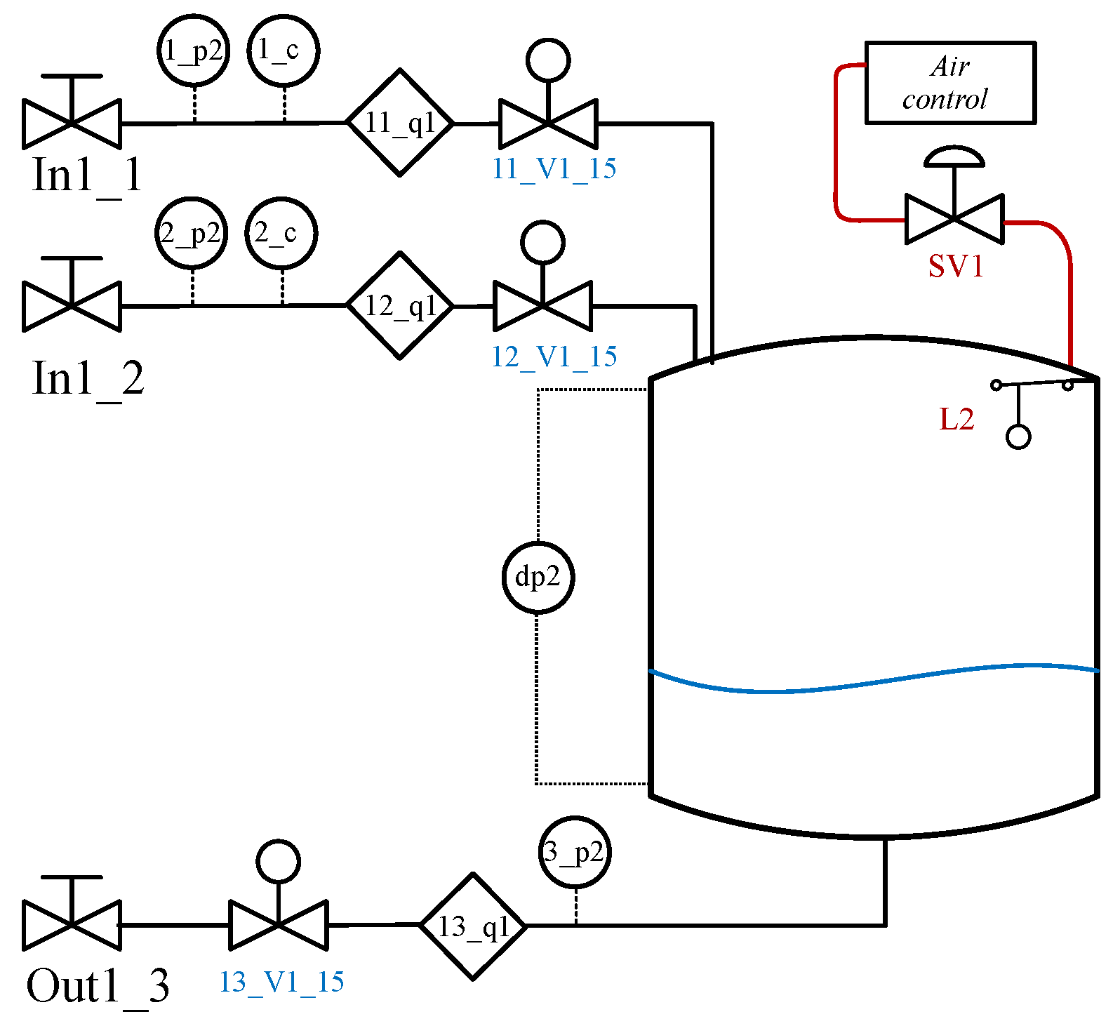
Figure A3.
Piping and instrumentation diagram of the water consumer unit. The legend is shown in Figure A1 and the details for each component are listed in Table A1.

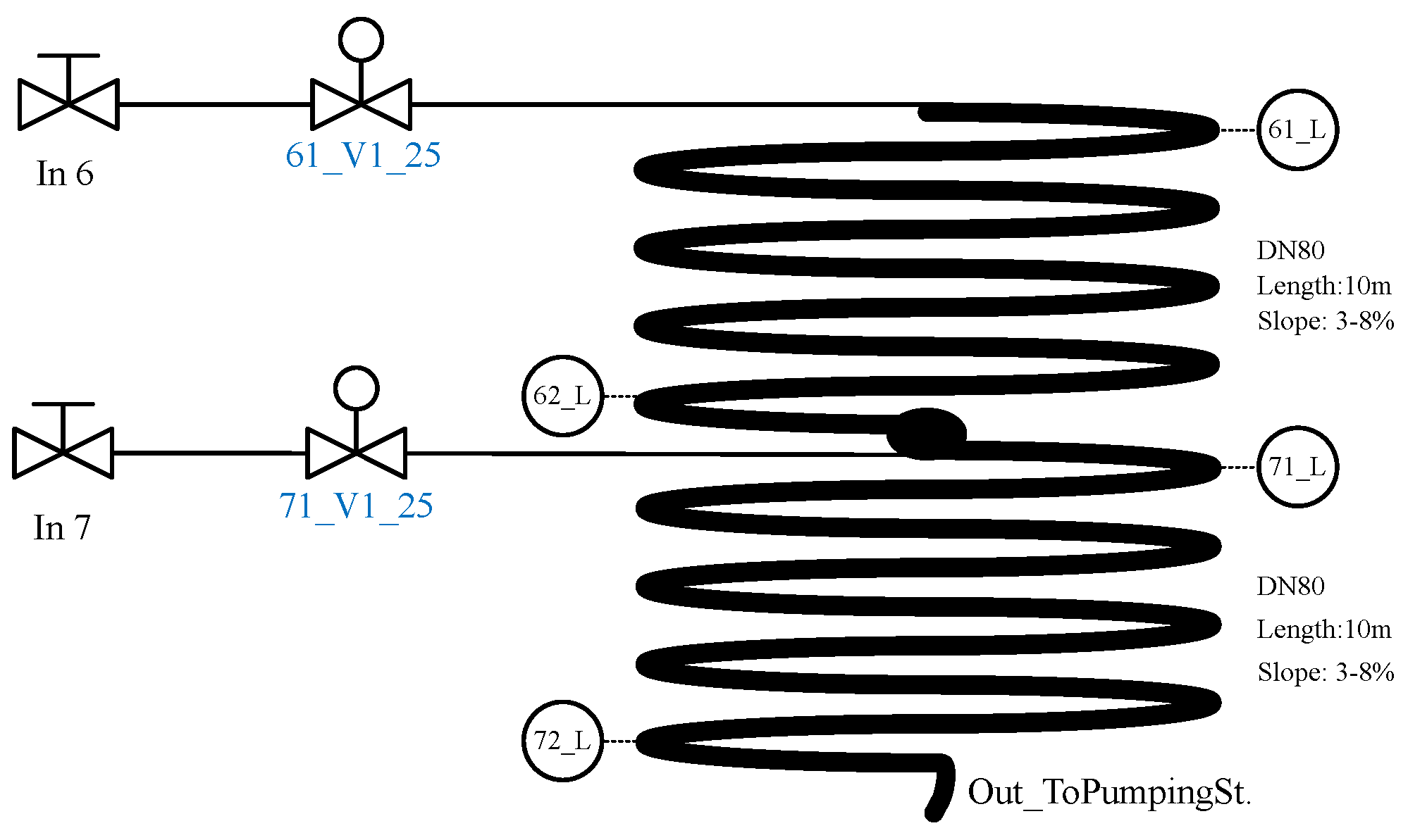
Figure A4.
Piping and instrumentation diagram of the sewer pipe unit. The legend is shown in Figure A1 and the details for each component are listed in Table A1.


References
- OECD. OECD Environmental Outlook to 2050; OECD: Paris, France, 2012. [Google Scholar]
- CPSoS. Analysis of the State-of-the-Art and Future Challenges in Cyber-Physical Systems of Systems; CPSoS 611115; European Union: Brussels, Belgium, 2015. [Google Scholar]
- Lund, H. Renewable energy strategies for sustainable development. Energy 2007, 32. [Google Scholar] [CrossRef] [Green Version]
- GIZ. Guidelines for Water Loss Reduction—A Focus on Pressure Management; GIZ: Bonn, Germany, 2011. [Google Scholar]
- Environmental Protection Agency. Smart Data Infrastructure for Wet Weather Control and Decision Support; Technical Report; EPA: Washington, DC, USA, 2021.
- Arnbjerg-Nielsen, K.; Willems, P.; Olsson, J.; Beecham, S.; Pathirana, A.; Bülow Gregersen, I.; Madsen, H.; Nguyen, V.T.V. Impacts of climate change on rainfall extremes and urban drainage systems: A review. Water Sci. Technol. 2013, 68, 16–28. [Google Scholar] [CrossRef] [PubMed]
- OECD. Diffuse Pollution, Degraded Waters; OECD: Paris, France, 2017; p. 120. [Google Scholar] [CrossRef]
- Environmental Protection Agency. Effects of Water Age on Distribution System Water Quality; Technical Report; EPA: Washington, DC, USA, 2007.
- Kowalska, B.; Kowalski, D.; Musz-Pomorska, A. Chlorine decay in water distribution systems. Environ. Prot. Eng. 2006, 32, 5–16. [Google Scholar]
- World Health Organization. Water Safety in Distribution Systems; World Health Organization: Geneva, Switzerland, 2014. [Google Scholar]
- Dadson, S.J.; Garrick, D.E.; Penning-Rowsell, E.C.; Hall, J.W.; Hope, R.; Hughes, J. (Eds.) Water Science, Policy, and Management: A Global Challenge, 1st ed.; Wiley: Hoboken, NJ, USA, 2019. [Google Scholar] [CrossRef]
- Adedeji, K.B.; Hamam, Y.; Abu-Mahfouz, A.M. Impact of Pressure-Driven Demand on Background Leakage Estimation in Water Supply Networks. Water 2019, 11, 1600. [Google Scholar] [CrossRef] [Green Version]
- Bosco, C.; Campisano, A.; Modica, C.; Pezzinga, G. Application of Rehabilitation and Active Pressure Control Strategies for Leakage Reduction in a Case-Study Network. Water 2020, 12, 2215. [Google Scholar] [CrossRef]
- Wu, Z.; Sage, P. Pressure dependent demand optimization for leakage detection in water distribution systems. In Water Management Challenges in Global Change; Taylor & Francis: Oxfordshire, UK, 2007; pp. 353–361. [Google Scholar]
- Morosini, A.F.; Veltri, P.; Costanzo, F.; Savić, D. Identification of leakages by calibration of WDS models. Procedia Eng. 2014, 70, 660–667. [Google Scholar] [CrossRef] [Green Version]
- Jensen, T.; Kallesøe, C. Application of a Novel Leakage Detection Framework for Municipal Water Supply on AAU Water Supply Lab. In Proceedings of the 2016 3rd Conference on Control and Fault-Tolerant Systems (SysTol), Barcelona, Spain, 7–9 September 2016; IEEE: Piscataway, NJ, USA, 2016; pp. 428–433. [Google Scholar] [CrossRef]
- Bendtsen, J.; Val, J.; Kallesøe, C.; Krstic, M. Control of District Heating System with Flow-dependent Delays. IFAC-PapersOnLine 2017, 50, 13612–13617. [Google Scholar] [CrossRef]
- Sakomoto, T.; Lutaaya, M.; Abraham, E. Managing Water Quality in Intermittent Supply Systems: The Case of Mukono Town, Uganda. Water 2020, 12, 806. [Google Scholar] [CrossRef] [Green Version]
- García, L.; Barreiro-Gomez, J.; Escobar, E.; Téllez, D.; Quijano, N.; Ocampo-Martinez, C. Modeling and real-time control of urban drainage systems: A review. Adv. Water Resour. 2015, 85, 120–132. [Google Scholar] [CrossRef] [Green Version]
- Mollerup, A.; Mikkelsen, P.; Sin, G. A methodological approach to the design of optimising control strategies for sewer systems. Environ. Model. Softw. 2016, 83, 103–115. [Google Scholar] [CrossRef] [Green Version]
- Lund, N.; Falk, A.K.; Borup, M.; Madsen, H.; Mikkelsen, P. Model predictive control of urban drainage systems: A review and perspective towards smart real-time water management. Crit. Rev. Environ. Sci. Technol. 2018, 48, 1–61. [Google Scholar] [CrossRef]
- Roche, S.; Nabian, N.; Kloeckl, K.; Ratti, C. Are ‘Smart Cities’ Smart Enough? In Spatially Enabling Government, Industry and Citizens: Research Development and Perspectives; GSDI Association Press: Needham, MA, USA, 2012; pp. 215–236. [Google Scholar]
- Eggimann, S.; Mutzner, L.; Wani, O.; Schneider, M.; Spuhler, D.; Moy de Vitry, M.; Beutler, P.; Maurer, M. The Potential of Knowing More: A Review of Data-Driven Urban Water Management. Environ. Sci. Technol. 2017, 51. [Google Scholar] [CrossRef] [PubMed] [Green Version]
- Kerkez, B.; Gruden, C.; Lewis, M.; Montestruque, L.; Quigley, M.; Wong, B.; Bedig, A.; Kertesz, R.; Braun, T.; Cadwalader, O.; et al. Smarter Stormwater Systems. Environ. Sci. Technol. 2016, 50. [Google Scholar] [CrossRef]
- Nikolopoulos, D.; Ostfeld, A.; Salomons, E.; Makropoulos, C. Resilience Assessment of Water Quality Sensor Designs under Cyber-Physical Attacks. Water 2021, 13, 647. [Google Scholar] [CrossRef]
- Tuptuk, N.; Hazell, P.; Watson, J.; Hailes, S. A Systematic Review of the State of Cyber-Security in Water Systems. Water 2021, 13, 81. [Google Scholar] [CrossRef]
- Madsen, O.; Møller, C. The AAU Smart Production Laboratory for Teaching and Research in Emerging Digital Manufacturing Technologies. Procedia Manuf. 2017, 9, 106–112. [Google Scholar] [CrossRef]
- Aicher, T.; Regulin, D.; Schütz, D.; Lieberoth-Leden, C.; Spindler, M.; Günthner, W.; Vogel-Heuser, B. Increasing flexibility of modular automated material flow systems: A meta model architecture. IFAC-PapersOnLine 2016, 49, 1543–1548. [Google Scholar] [CrossRef]
- Eurac. Eurac Research, Ifrastructure Labs. 1992. Available online: http://www.eurac.edu (accessed on 14 April 2019).
- iTrust. Itrust—Singapore University of Technology and Design. 2017. Available online: https://itrust.sutd.edu.sg/ (accessed on 14 April 2019).
- Kallesøe, C. Fault Detection and Isolation in Centrifugal Pumps. Ph.D. Thesis, Aalborg University, Aalborg Øst, Denmark, 2005. [Google Scholar]
- Swamee, P.K.; Sharma, A.K. Design of Water Supply Pipe Networks; Wiley: Hoboken, NJ, USA, 2008. [Google Scholar] [CrossRef]
- Schuetze, M.; Butler, D.; Beck, M. Modelling, Simulation and Control of Urban Wastewater Systems; Springer: Berlin/Heidelberg, Germany, 2002. [Google Scholar] [CrossRef]
- Litrico, X.; Fromion, V. Modeling and Control of Hydrosystems; Springer: Berlin/Heidelberg, Germany, 2009. [Google Scholar]
- Te Chow, V. Open Channel Hydraulics; McGraw-Hill International Book Company: New York, NY, USA, 1982. [Google Scholar]
- Boysen, H. kv: What, Why, How, Whence? Technical Paper; Danfoss A/S: Nordborg, Denmark, 2009; Available online: https://assets.danfoss.com/documents/90621/AC026186467824en-010201.pdf (accessed on 4 July 2021).
- Val, J. GitHub repository, SWIL. 2021. Available online: https://github.com/jvledesma/SWIL (accessed on 26 March 2021).
- Maschler, T.; Savic, D.A. Simplification of Water Supply Network Models through Linearisation; Technical Report 99/01; University of Exeter: Exeter, UK, 1999. [Google Scholar]
- Bizier, P. (Ed.) Gravity Sanitary Sewer Design and Construction; ASCE manuals and reports on engineering practice; American Society of Civil Engineers: Reston, VA, USA, 2007. [Google Scholar]
- 3S-Smart Software Solutions GmbH. CODESYS V3.5 SP14. Available online: https://www.codesys.com (accessed on 19 December 2018).
- Rathore, S.S. Nonlinear Optimal Control in Water Distribution Network. Master’s Thesis, Aalborg University, Aalborg, Denmark, 2020. [Google Scholar]
- Val, J.; Wisniewski, R.; Kallesøe, C. Safe Reinforcement Learning Control for Water Distribution Networks. In Proceedings of the Conference on Control Technology and Applications, San Diego, CA, USA, 8–11 August 2021; IEEE: Piscataway, NJ, USA, 2021. [Google Scholar]
- Nielsen, K.; Pedersen, T.; Kallesøe, C.; Andersen, P.; Mestre, L.; Murigesan, P. Control of Sewer Flow Using a Buffer Tank. In Proceedings of the 17th International Conference on Informatics in Control, Automation and Robotics, Paris, France, 7–9 July 2020; pp. 63–70. [Google Scholar] [CrossRef]
- Balla, K.; Knudsen, C.; Hodzic, A.; Bendtsen, J.; Kallesøe, C. Nonlinear Grey-box Identification of Gravity-driven Sewer Networks with the Backwater Effect. In Proceedings of the Conference on Control Technology and Applications, San Diego, VA, USA, 8–11 August 2021; IEEE: Piscataway, NJ, USA, 2021. [Google Scholar]
Figure 1.
Picture of the SWIL with two test-beds and the SCADA-PC: (Left) Waste water collection. (Center) Water distribution network. (Right) SCADA-PC.
Figure 1.
Picture of the SWIL with two test-beds and the SCADA-PC: (Left) Waste water collection. (Center) Water distribution network. (Right) SCADA-PC.

Figure 2.
Sketches of two water infrastructures: (Left) A water distribution network. (Right) A wastewater transport system.
Figure 2.
Sketches of two water infrastructures: (Left) A water distribution network. (Right) A wastewater transport system.

Figure 3.
Mechanical drawing of the pumping station tank.

Figure 4.
(Left) Illustration of a pressurised pipe, represents differential the elevation of the pipeline. (Right) Illustration of an open channel flow along a longitudinal axis x, represents the bed slope.
Figure 4.
(Left) Illustration of a pressurised pipe, represents differential the elevation of the pipeline. (Right) Illustration of an open channel flow along a longitudinal axis x, represents the bed slope.

Figure 5.
(Left): Scheme of a standard branched topology and its laboratory equivalent. (Right): Scheme of a standard ring topology and its laboratory equivalent.
Figure 5.
(Left): Scheme of a standard branched topology and its laboratory equivalent. (Right): Scheme of a standard ring topology and its laboratory equivalent.

Figure 6.
Diagram of the hydraulic network used as reference for the design of the modules with a single pumping station and three consumer units representing aggregated end-users in a city district.
Figure 6.
Diagram of the hydraulic network used as reference for the design of the modules with a single pumping station and three consumer units representing aggregated end-users in a city district.

Figure 7.
Graph of a pump curve extracted from the data-sheet of Grundfos-UPM3. The performance of PWM controlled pumps is measured with A profile (heating) at eight PWM values: 5% (max.), 20%, 31%, 41%, 52%, 62%, 73%, 88% (min.), PWM regulates the speed of the pumps .
Figure 7.
Graph of a pump curve extracted from the data-sheet of Grundfos-UPM3. The performance of PWM controlled pumps is measured with A profile (heating) at eight PWM values: 5% (max.), 20%, 31%, 41%, 52%, 62%, 73%, 88% (min.), PWM regulates the speed of the pumps .

Figure 8.
Sketch of a reference waste water collection with three discharge sources, district, rain, and industry, several retention tanks and a treatment plant.
Figure 8.
Sketch of a reference waste water collection with three discharge sources, district, rain, and industry, several retention tanks and a treatment plant.

Figure 9.
(Left): Simulation results of the Manning’s formula with different pipe sizing. (Center): Front view of the mechanical drawing of the gravity sewer. (Right): Top view of the mechanical drawing of the gravity sewer.
Figure 9.
(Left): Simulation results of the Manning’s formula with different pipe sizing. (Center): Front view of the mechanical drawing of the gravity sewer. (Right): Top view of the mechanical drawing of the gravity sewer.

Figure 10.
Scheme of the laboratory control and DAQ architecture.

Figure 11.
Communication network architecture of the SWIL that connects the CCU and LUs via TCP/IP Modbus.
Figure 11.
Communication network architecture of the SWIL that connects the CCU and LUs via TCP/IP Modbus.

Figure 12.
Map of Bjerringbro and its water distribution network scheme. Green and red blocks represent the main elements of the network which can be emulated with laboratory modules.
Figure 12.
Map of Bjerringbro and its water distribution network scheme. Green and red blocks represent the main elements of the network which can be emulated with laboratory modules.

Figure 13.
Diagram of the a ring topology water distribution network that is built with laboratory modules. This network is inspired by the structure from Figure 12.
Figure 13.
Diagram of the a ring topology water distribution network that is built with laboratory modules. This network is inspired by the structure from Figure 12.

Figure 14.
Graphs of real data collected by Bjerringbro´s water utility. The measurement nodes are represented in Figure 12 and the tank filling is regulated with a standard ON/OFF control.
Figure 14.
Graphs of real data collected by Bjerringbro´s water utility. The measurement nodes are represented in Figure 12 and the tank filling is regulated with a standard ON/OFF control.

Figure 15.
Graphs of the experimental results with non-linear MPC control applied to Bjerringbro’s study case [41].
Figure 15.
Graphs of the experimental results with non-linear MPC control applied to Bjerringbro’s study case [41].

Figure 16.
Graphs of the experimental results with RL control applied to Bjerringbro’s study case [42].
Figure 16.
Graphs of the experimental results with RL control applied to Bjerringbro’s study case [42].

Figure 17.
Map of Fredericia and its waste water collection scheme. Green and red blocks represent the main elements of the network which are emulated with laboratory modules.
Figure 17.
Map of Fredericia and its waste water collection scheme. Green and red blocks represent the main elements of the network which are emulated with laboratory modules.

Figure 18.
Diagram of the emulated waste water collection at the SWIL.

Figure 19.
Graph from the experimental results of Fredericia’s study case [43]. The graph shows a comparison of the inlet flow at the treatment plant (sensor L) between non-controlled industry discharge and a controlled one with MPC.
Figure 19.
Graph from the experimental results of Fredericia’s study case [43]. The graph shows a comparison of the inlet flow at the treatment plant (sensor L) between non-controlled industry discharge and a controlled one with MPC.

Figure 20.
Map of Ishøj and its waste water collection scheme. (Right) The complete network model. (Left) A section of the sewer with two tanks or open basins and a smaller sewer conveys to the main sewer. Green and red blocks represent the main elements of the network which are emulated with laboratory modules.

Figure 21.
Diagram of the Ishøj emulated waste water collection at the SWIL.

Figure 22.
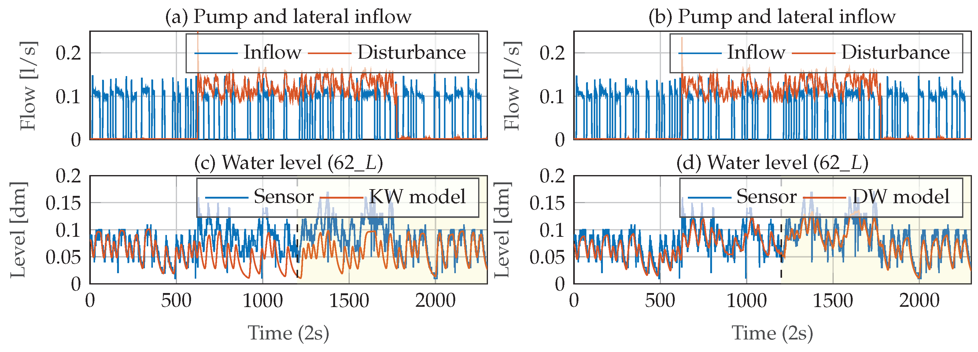
Graph from the experimental results of Ishøj’s study case [44], where the first part represents the system identification (training) and the second, in yellow, represents the validation.
Figure 22.
Graph from the experimental results of Ishøj’s study case [44], where the first part represents the system identification (training) and the second, in yellow, represents the validation.

Publisher’s Note: MDPI stays neutral with regard to jurisdictional claims in published maps and institutional affiliations. |
© 2021 by the authors. Licensee MDPI, Basel, Switzerland. This article is an open access article distributed under the terms and conditions of the Creative Commons Attribution (CC BY) license (https://creativecommons.org/licenses/by/4.0/).
Share and Cite
MDPI and ACS Style
Val Ledesma, J.; Wisniewski, R.; Kallesøe, C.S. Smart Water Infrastructures Laboratory: Reconfigurable Test-Beds for Research in Water Infrastructures Management. Water 2021, 13, 1875. https://doi.org/10.3390/w13131875
AMA Style
Val Ledesma J, Wisniewski R, Kallesøe CS. Smart Water Infrastructures Laboratory: Reconfigurable Test-Beds for Research in Water Infrastructures Management. Water. 2021; 13(13):1875. https://doi.org/10.3390/w13131875
Chicago/Turabian StyleVal Ledesma, Jorge, Rafał Wisniewski, and Carsten Skovmose Kallesøe. 2021. "Smart Water Infrastructures Laboratory: Reconfigurable Test-Beds for Research in Water Infrastructures Management" Water 13, no. 13: 1875. https://doi.org/10.3390/w13131875
Note that from the first issue of 2016, this journal uses article numbers instead of page numbers. See further details here.