
The Response of the HydroGeoSphere Model to Alternative Spatial Precipitation Simulation Methods

1
State Key Laboratory of Hydrology-Water Resources and Hydraulic Engineering, College of Hydrology and Water Resources, Hohai University, Nanjing 210098, China
2
The Huaihe River Commission of the Ministry of Water Resource, Bengbu 233001, China
3
Department of Agronomy, Iowa State University, Ames, IA 50011, USA
*
Author to whom correspondence should be addressed.
Water 2021, 13(14), 1891; https://doi.org/10.3390/w13141891
Submission received: 28 May 2021
/
Revised: 4 July 2021
/
Accepted: 5 July 2021
/
Published: 8 July 2021
(This article belongs to the Special Issue Human and Climate Impacts on Drought Dynamics and Vulnerability)
Abstract
:This paper presents the simulation results obtained from a physically based surface-subsurface hydrological model in a 5730 km2 watershed and the runoff response of the physically based hydrological models for three methods used to generate the spatial precipitation distribution: Thiessen polygons (TP), Co-Kriging (CK) interpolation and simulated annealing (SA). The HydroGeoSphere model is employed to simulate the rainfall-runoff process in two watersheds. For a large precipitation event, the simulated patterns using SA appear to be more realistic than those using the TP and CK method. In a large-scale watershed, the results demonstrate that when HydroGeoSphere is forced by TP precipitation data, it fails to reproduce the timing, intensity, or peak streamflow values. On the other hand, when HydroGeoSphere is forced by CK and SA data, the results are consistent with the measured streamflows. In a medium-scale watershed, the HydroGeoSphere results show a similar response compared to the measured streamflow values when driven by all three methods used to estimate the precipitation, although the SA case is slightly better than the other cases. The analytical results could provide a valuable counterpart to existing climate-based drought indices by comparing multiple interpolation methods in simulating land surface runoff.
1. Introduction
In the past decades, hydrological models have been developed to simulate hydrological variables and water cycles [1]. It is an open issue whether these models are suitable to capture hydrological drought, in terms of soil moisture, runoff, and evaporation. Compared to soil moisture and evaporation, runoff is closer to being a verified product from models [2]. Therefore, using runoff-based indexes such as standardized runoff index (SRI) to analyze drought behavior is a reliable way to be applied in hydrological drought researches. As to runoff simulation, several articles have discussed the use of physically based hydrological models to simulate the hydrologic response of surface and subsurface systems to transient precipitation events. Significant progress has been achieved in improving the accuracy and efficiency of physically based hydrological models, especially in the last ten years. Many researchers have exceeded the goals outlined in the Freeze and Harlan [3] blueprint, and there has been several comprehensive physically based hydrological models developed such as InHM [4], MODHMS [5,6], and HydroGeoSphere [7,8], to name a few, although applications were limited to small sub-basins or experimental field sites [4,9,10,11,12,13]. When applying a physically based hydrological model to a large watershed (Area > 1000 km2), there are still many issues that need to be addressed.
For a large watershed, a lumped model or a semi-distributed hydrological model is often employed to simulate the rainfall-runoff process [14], because it is a simple approach that usually requires fewer input parameters, generally runs in less CPU time than a physically based hydrological model, and is easy to understand. As such it has become a popular tool for flood forecasting as one example. However, the physically based hydrological models offer many advantages when compared to lumped models, such as analyzing the spatial variability of precipitation, infiltration, etc. These problems are of increasing concern to scientists and planners [15]. However, it is a challenging problem to determine how a physically based hydrological model can be used in large watersheds (Area km2) when driven by uncertain precipitation patterns over large areas.
Recently, there have been some physically based hydrological models applied to medium-sized watersheds, such as by Jones, Sudicky [16] (area: 75 km2), Li, Unger [15] (area: 285.6 km2), Goderniaux, Brouyre [17] (area: 480 km2). When the basin is relatively large (over thousands of square kilometers) many issues need to be considered when physically based hydrological models are used to simulate the rainfall-runoff process, including (1) uncertainty in the model output arising from uncertainty in the input data (measurement and interpolation errors) and in the models themselves (conceptual, logical, mathematical, and computational errors) and (2) the limited computational capacity available to many users. The growing trend of model complexity, data availability, and physical representation has always pushed the limits of computational efficiency, which in turn has limited the application of physically based hydrological models to small domains and for shorter durations [18]. To our knowledge, the use of a fully integrated physically based hydrological model to simulate the rainfall-runoff process over thousands of square kilometers is rare.
In a fully integrated, distributed hydrological model, the high-precision precipitation data are the key input that drives the hydrologic process, but if the watershed gauge site is scarce, remote sensing precipitation product is coarse, it is very important to get the high precision precipitation product using the interpolation method to improve the accuracy of the rainfall-runoff process simulation.
Currently, the most widely used method for obtaining the spatial distribution of precipitation involves the interpolation of observed precipitation data coupled with additional information obtained from topography, satellite, and radar data [19,20,21,22,23].
Bárdossy and Pegram [23] compared four measures of interpolation quality and they find that a copula-based method is better than the ordinary and external drift Kriging method for monthly and daily scales. Similarly, several studies have demonstrated that the inverse distance weighted (IDW) method is one of the most used deterministic interpolation methods to reproduce rainfall fields [24,25,26,27]. For hourly scale, Moulin and Gaume [28] investigated the interpolation uncertainty of hourly precipitation amounts. They proposed an error model that considers the temporal dependence of the errors. Further, and significantly, they conclude that precipitation uncertainty is possibly the most important source for rainfall/runoff model errors.
A number of authors evaluated the performance of Kriging in the mapping of precipitation [29,30,31], finding good performance of this interpolator based on small mean error generated by the cross-validation, and on the strong spatial dependence presented by the semivariograms.
The disadvantage of interpolation is the loss of variability, i.e., small values will be over-estimated and large values will be under-estimated [32], which may result in relatively large errors, particularly in flood forecasting where extreme rainfall values determine the model output. Therefore, in such situations, the spatial stochastic simulation of a random variable (e.g., by Gaussian sequential simulation, turning bands method, simulated annealing, etc.) is usually employed to generate the spatial precipitation distribution [32,33].
So, an understanding of the impact that various precipitation interpolation methods have on the performance of the physically based hydrological model is very important. Moreover, the comparative use of alternative interpolation methods to estimate rainfall as input for a physically based hydrological model has been very little studied [12,31,34].
In this paper, the main objective is to study the response of the HGS (HydroGeoSphere) model to different spatial precipitation interpolation methods. The HGS model will be applied to the Shiguan River basin of China.
2. The Study Area
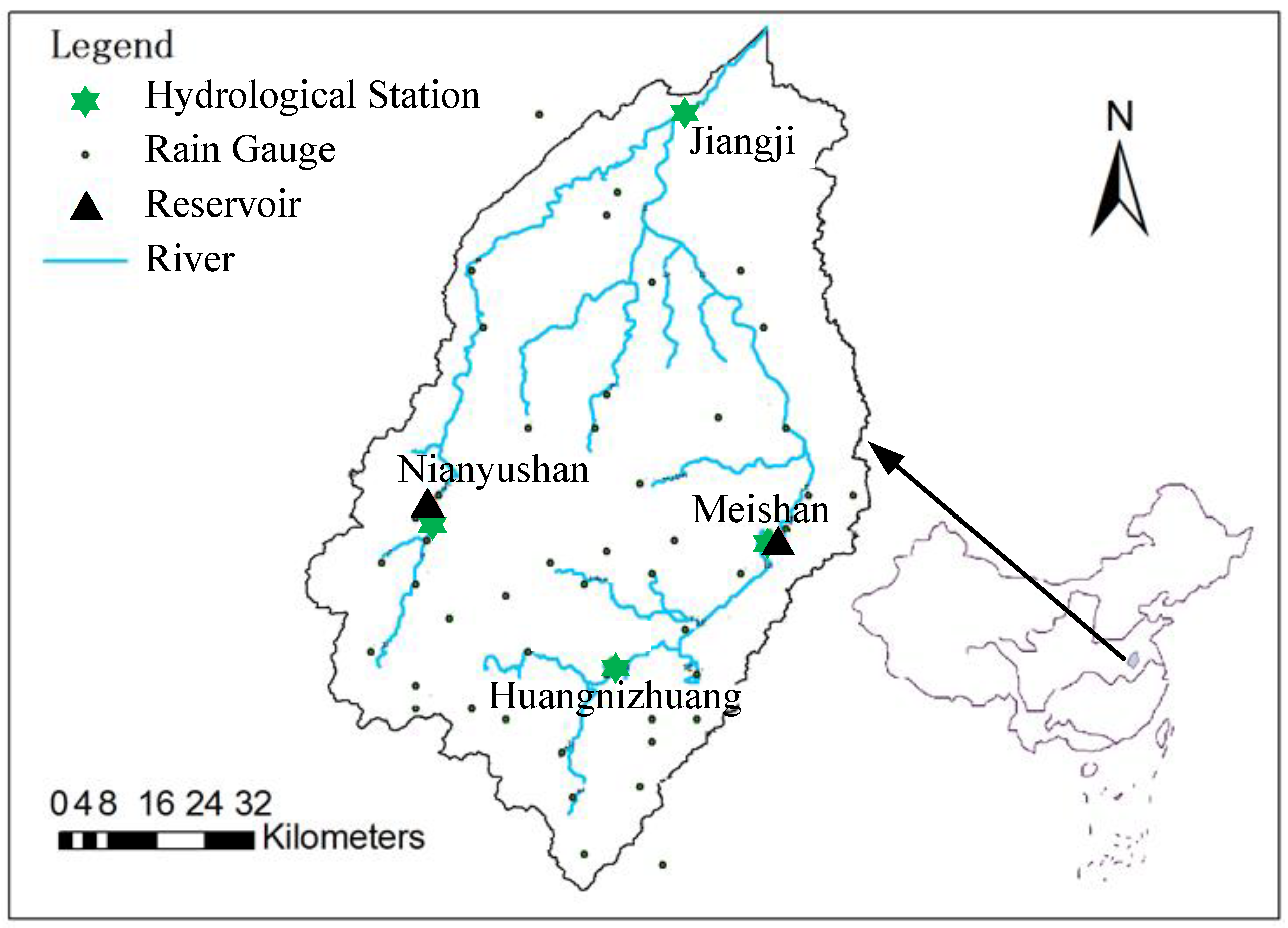
The Shiguan river basin (Figure 1) is located in the southern part of the Huai River Basin and is a closed basin. The catchment area is approximately 5730 km2 and Jiangji is the basin outlet. The basin slopes from south to north with the elevation changing from 1536 to 18.7 m over a horizontal extent of about 128 km. It is an important tributary of the Huai River and originates from the northern slope of the Dabie Mountain in the south Huai River Basin. The river system has two major tributaries: the Shi River to the east and the Guan River to the west, and they merge near the Jiangji outlet (Figure 1). The two tributaries are regulated by the Meishan and Nianyushan reservoirs that have watershed areas of 1970 and 924 km2 respectively, with corresponding travel distances of 88 and 89 km from the reservoir outflow point to the Jiangji outlet.
Climatologically, the basin lies in the warm semihumid monsoon region. The sub-basin exhibits a diversified natural topography, land surface cover, soil texture, hydrogeology, hydrology, and climatology. Precipitation mainly occurs in the period from mid-May to mid-October, and basin-wide flooding is common during the rainy season and is caused by anomalies of the Meiyu front, which is in turn influenced by the South Asian monsoon. However, this area often suffers from drought events in flood season (June to September), hence the variation of runoff could help for local agricultural management, i.e., drought monitoring and irrigation strategies.
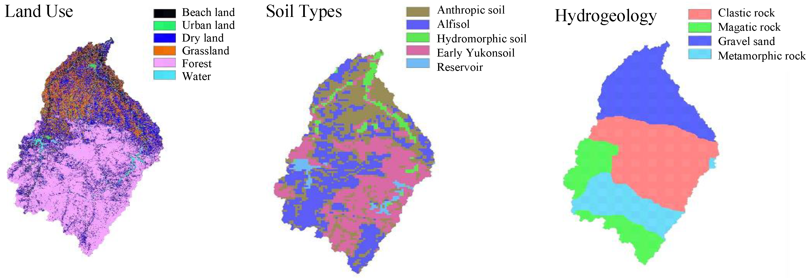
Soil types in the mountainous upstream region are predominantly anthrosols (paddy soils), luvisols (brown soil), semi-hydromorphic soils (cinnamonic soil, black soil), entisols (soils whose parent materials are weathered rock, alluvium, or artificial heap pad materials), and saline soils. Soil types in the lowland downstream region area mainly paddy soils derived from Quaternary-aged lacustrine deposits. The China regional soil type classification database developed by the Institute of Soil Science, Chinese Academy of Sciences (http://vdb3.soil.csdb.cn/, last accessed date: 28 May 2021) is used to determine the soil type and soil parameters in the basin, shown in Figure 2. Soil thickness data comes from the book “Chinese soil species records” Volume 1–6. The CK method was used to interpolate a continuous soil thickness distribution over a grid of 1 × 1 km2 resolution.
The Shiguan river basin has been subdivided into four unique zones of hydrogeologic significance, as shown in Figure 2. The China regional hydrogeology classification database, developed by the Ministry of Geology and Mineral Resources of P.R. China (http://www.ngac.cn/, last accessed date: 28 May 2021) was used to determine the hydrogeologic type and parameters in the basin.
A digital elevation model (DEM) from the ASTER Global Digital Elevation Map is used to set up the flow routing network over the sub-basin. The University of Maryland 1-km Global Land Cover Classification data together with the look-up table in [35,36] are used to create the land use type data.
The intensive operating period of the Huai river basin experiment of the global energy and water cycle experiment of the Asian monsoon experiment was carried out mainly over the Shiguan river basin during the summers of 1998 and 1999 [37,38,39]. The intensive operating period data are provided by the Information Center of the Chinese Ministry of Water Resources. There are 48 rain gauges (Figure 1) covering the Shiguan river sub-basin and a long-term flux monitoring station located at Shouxian. Streamflows were measured at the Jiangji and Huangnizhuang hydrology stations. The precipitation was measured every hour, while streamflow was observed every three hours. The HGS model was a spin-up model. The spin-up period was from 1 May 1998 to 31 August 1998. The simulated period begins on May 1 and ends on 30 August 1999. The rainfall drive is hourly scale data, and the model outputs are hourly scale data too. Runoff observations are 3 h scale data. Rainfall-driven data are hourly, and the model outputs hourly data. Runoff observations are 3 h scale data.
The spatial precipitation data used to drive the transient hydrological model comes from three methods: (1) average value using TP rules for the 48 gauge stations (TP method); (2) spatial interpolation precipitation using CK for the 48 gauge stations for a 5 5 km2 resolution (CK method); (3) the simulated spatial precipitation distribution for a 5 5 km2 resolution using the simulated annealing algorithm (SA method).
In addition, the Shiguan river basin’s upstream Huangnizhuang portion (area: 808 km2) was also selected to study the impact of the rainfall distribution methods on a medium-scale.
3. Methodology
3.1. The Physically Based Hydrological Model
A hydrological model was performed with the HGS hydrological model [7,15,16,40]. HGS simulates an integrated system of 3D variably saturated groundwater flow in porous and/or discretely-fractured porous media coupled with 2D overland flow over the land surface. A detailed description of the mathematical basis of HGS can be found in Therrien and Sudicky [41] (subsurface flow); VanderKwaak and Loague [4]; Panday and Huyakorn [6] (surface flow); Panday and Huyakorn [6] (evapotranspiration); Aquanty-Inc [7] (comprehensive user guide).
3.2. Discretisation, Boundary Conditions, and Computational Process
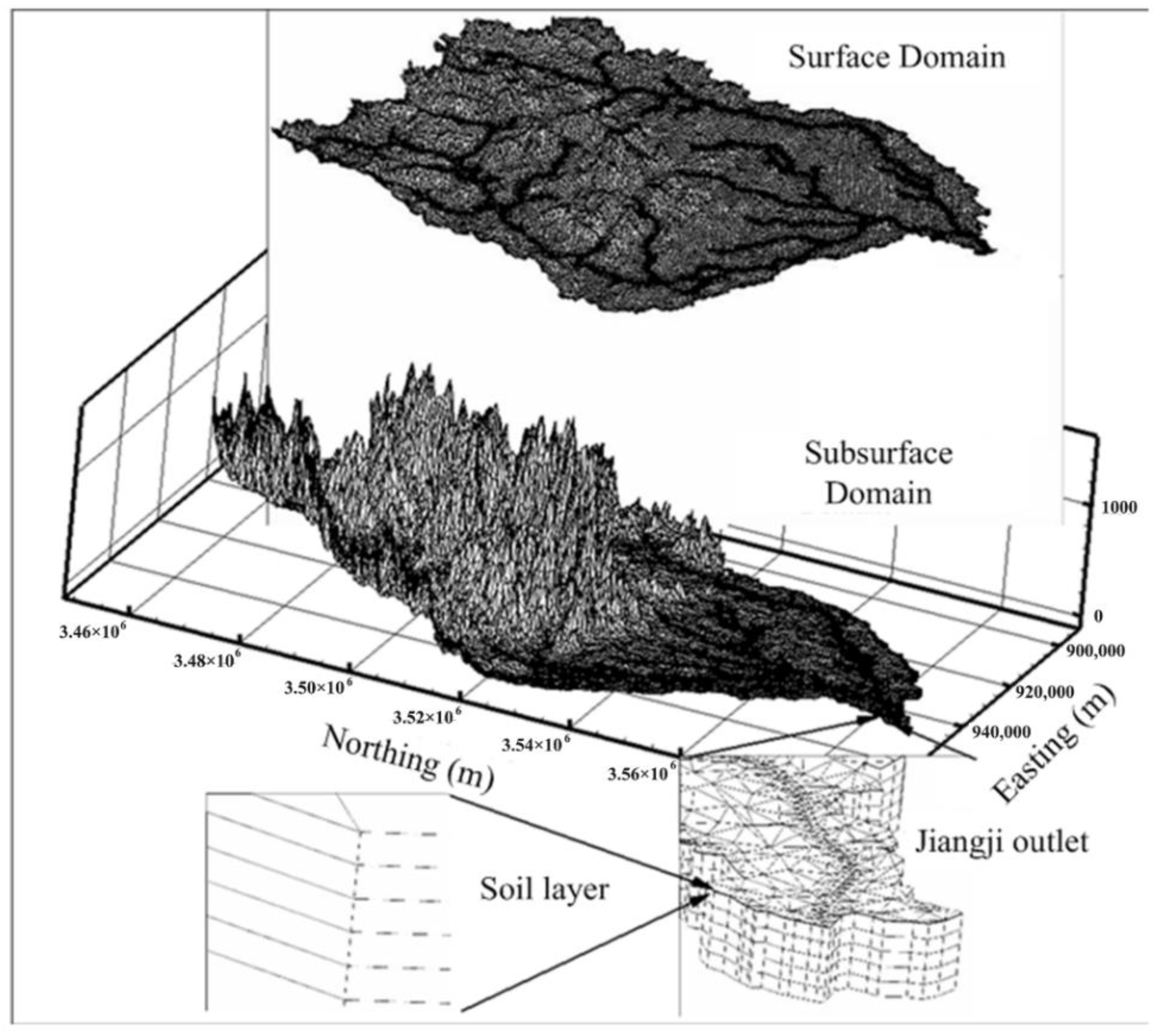
A three-dimensional finite element mesh, composed of 11 layers of six-node triangular prismatic elements was generated (Figure 3). The elements have lateral dimensions equal to approximately 500 m on average, but the lateral dimensions are variable because an unstructured mesh is used. For example, in rivers and reservoirs, the mesh is refined such that element sides do not exceed a length of 100 m. The top layer of nodes, defined by the DEM, represents the soil surface. We assume that the base of the domain is an impermeable boundary and is defined in the model as a flat plane.
Subsurface formations are discretized using 11 finite element layers. The top five layers are distributed uniformly over the first 1 m below the ground surface, with each layer having a thickness of 0.2 m. The vertical thickness of these layers is relatively small so that the exchange of soil moisture between layers can be more accurately described. In the upper 0–2 m of the domain, in addition to the movement of soil moisture, plant-water root uptake processes are also accounted for.
The thickness of the remaining lower layers is evenly distributed between the fifth and bottom layers. The physical parameters of each layer are taken from local observations or are derived from the literature. The CK interpolation method is employed to interpolate values at every node. The key parameters are calibrated according to the observed groundwater heads. The ground surface is used to define the 2D surface flow grid (Figure 3), and the elevation of each surface node is calculated from a DEM raster file with a 30 m resolution. The total number of surface nodes is 53,607. The total number of surface elements is 105,601.
The zero-flux boundary condition is applied to the subsurface nodes belonging to the western, southern, eastern, and bottom boundaries. Cauchy conditions (head-dependent flux) are applied on the subsurface nodes along the Jiangji outlet (northern boundary) to take into account groundwater losses in the direction of the adjacent catchment located north of the Shiguan river basin. No-flow Neumann boundary conditions are applied along naturally occurring hydrologic limits of the Shiguan river basin for the surface flow domain. Critical-depth boundary conditions are prescribed at the nodes corresponding to the catchment outlet, at the location of the Jiangji gauging station.
In the subsurface domain, the hydraulic head and the Darcy flux are computed at each node. In the surface domain, the water depth and the fluid flux at each node in the 2D grid are calculated at each time step. The Newton–Raphson method is used to solve the system of nonlinear equations [5]. The fully-integrated set of nonlinear discrete equations is linearized using Newton–Raphson schemes and is solved simultaneously in an iterative fashion at every time step. The Newton–Raphson technique is used to linearize the nonlinear equations arising from the discretization of variably saturated subsurface or surface flow equations. The method is described in [6] and is reproduced here to demonstrate the advantage of using the control volume finite element approach over a conventional Galerkin method. A Newton–Raphson linearization package provides improved robustness. The hydrologic parameters required in the HGS model are listed in Table 1.
Water exchange fluxes between the corresponding surface and subsurface nodes are calculated from the hydraulic head differences between the two domains multiplied by a leakance factor characterizing the properties of the surface soil. The model of Kristensen and Jensen [42] is used to calculate the actual transpiration and actual evaporation .
3.3. Spatially-Distributed Precipitation Patterns
Three methods, TP, CK and SA, were used to generate spatially-distributed precipitation patterns over the Shiguan river basin using the data from the 48 rainfall gauges. TP is one of the most widely used and the simplest geostatistical method for spatial rainfall [43]. It calculates the weight of each rain gauge according to the rain gauge location to create a polygon network, and applies the gauge rainfall quantity over the polygon area. The weights of rain gauges are calculated according to the rain gauge location.
The Thiessen polygon approach is probably the most common method used in hydrometeorology for determining average precipitation (or snow) over an area when there is more than one measurement. The basic concept is to divide the watershed into several polygons, each one around a measurement point, and then take a weighted average of the measurements based on the size of each one’s polygon, i.e., measurements within large polygons are given more weight than measurements within small polygons.
In the study, a Thiessen polygon based on 48 rain gauge stations was defined, resulting in 21 areas of various sizes within which precipitation is assumed uniform. The precipitation amount for each rain gauge was corrected using actual gauge catch corrections.
CK is an extension of ordinary Kriging to situations where two (or more) variables are spatially intercorrelated. In this paper, only one covariable (DEM) is used [44]. Co-Kriging is a weighted average of observed values of the primary variable (the variable of immediate interest, e.g., precipitation) and the Co-variable . The estimated value of the primary variable at location is:
where and are the number of neighbor of and ; and are the weights associated to each sampling point. The weights are chosen to minimize the Co-Kriging variance by solving the Co-Kriging system
The auto- and cross-semivariograms are used the same semivariogram model (i.e., exponential model):
![Water 13 01891 i001]() where is the nugget variance, is the sill, 3a is the effective range of influence, and
where is the nugget variance, is the sill, 3a is the effective range of influence, and ![Water 13 01891 i002]() = |h| for the isotropic case.
= |h| for the isotropic case.

 = |h| for the isotropic case.
Range, sill and nugget in Equation (5) are simulated using the observed data. The nugget effects and partial sills must satisfy , for , where and are the nugget effects for variable and , and are the partial sills for variable and , and finally and are the nugget effect and partial sill for the cross-semivariogram. The Co-Kriging variance at the location is given by:
where is auto-semivariograms, is the cross-semivariogram and are Lagrange multipliers. and are the weights associated with each sampling point.
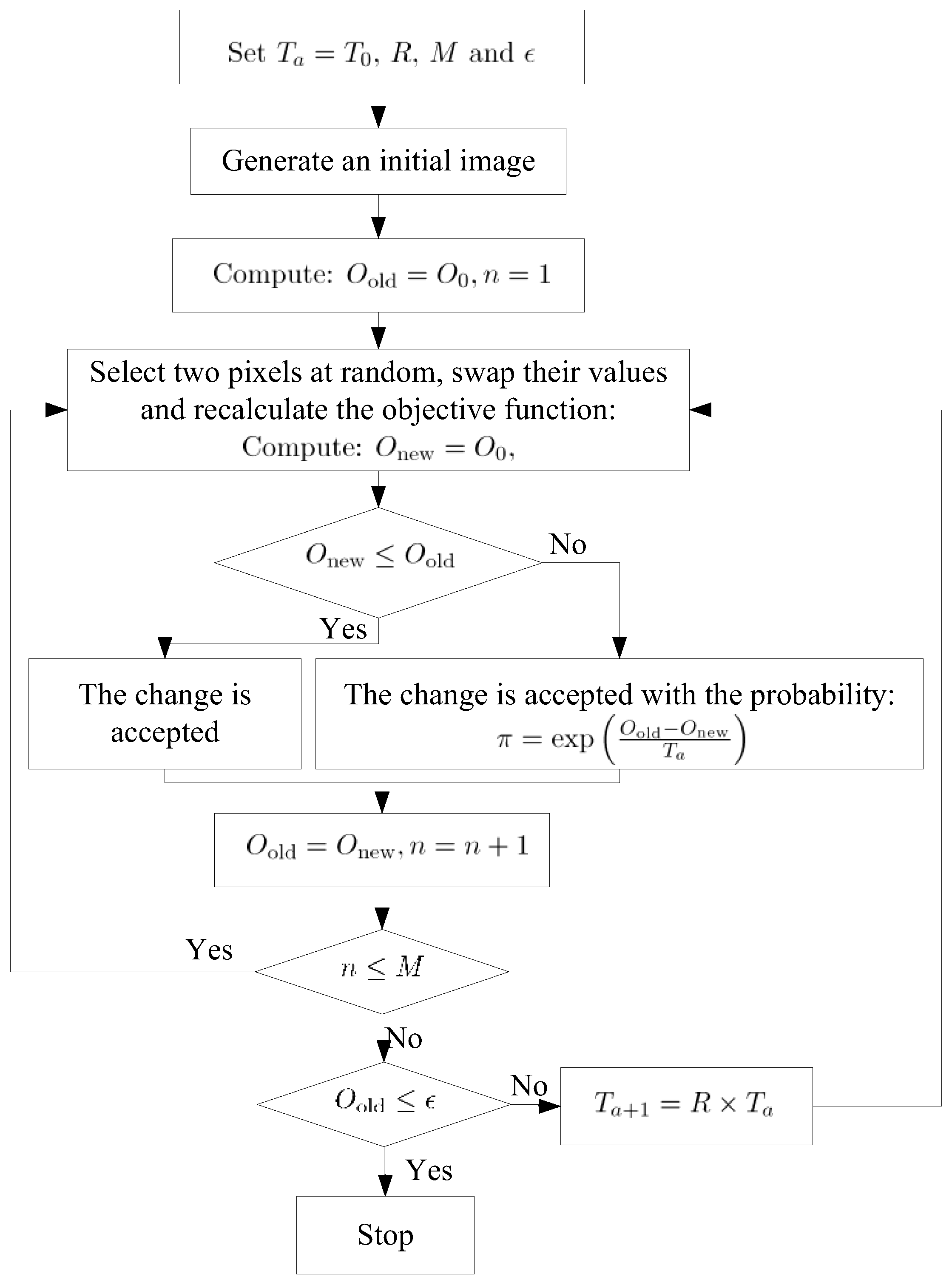
Simulated annealing (SA) is a generic probabilistic meta-algorithm for the global optimization problem. It was first introduced by Kirkpatrick, Gelatt [45]. In this paper, the simulated annealing method is employed for minimizing the objective function (Equation (6)). The energy of the annealing process is given by the value of the objective function (Equation (6)) and the temperature T [46].
- The initial weight coefficient.
- The energy is given by the objective function (Equation (6)), .
- The initial temperature is determined as: , where are the initial temperature and some parameters are selected (Figure 4).
- The initial configuration is perturbed by randomly selecting one from the rain gauges and the DEM locations, and the objective function is calculated.
- Let . If , the new configuration is accepted because the objective function has been minimized. However, if , the new configuration is accepted with probability acceptation criterion, and . If , step 4 is applied again.
- The temperature is decreased at a certain amount, , 0 < R < 1 and step 4 is applied again.
- The running of the simulation process is defined by steps 4–6 continues until:
- A number of prefixed numbers of iterations are reached;
- At a given constant T none of the numbers of new configurations have been accepted;
- Changes in the objective function for various consecutive steps are slight.
3.4. Calibration Procedure
An HGS model simulation requires the user to supply values for many physical parameters and an initial condition (groundwater hydraulic heads and surface water elevations) for a subsequent transient simulation. In this paper, the main parameters were obtained from the literature, field experiments, and optimization methods. The initial conditions are obtained from the steady-state simulation and spin-up process. Several steps are involved to determine the input parameters and to provide the initial condition.
Step 1. Parameters from references. In the surface flow domain, the Manning roughness coefficients () were assigned based on soil and land use maps. Five categories of land use, namely ‘beach’, ‘rural’, ‘dry land, ‘grass’, and ‘forest’ have been identified and roughness coefficient values were obtained from [16]. The surface-subsurface domain coupling length was assumed constant [15,17]. The parameters used to calculate the actual evapotranspiration [42] were taken from the literature for the various land-use categories [15,47]. During the simulation period, we assume a constant value for LAI. Values for the empirical transpiration fitting parameters , and as well as for the canopy storage interception were taken from Kristensen and Jensen [42] and Li, Unger [15].
Step 2. Parameters from experiments and simulation. In the subsurface domain, each of the hydrostratigraphic units was assumed to be homogenous throughout the study area in terms of their hydrogeological properties. The subsurface system is divided into two layers: a soil layer and a rock layer. In the soil layer, particle size distributions and bulk porosity values for each different soil type were measured in the laboratory and then used in the Rosetta software [48] to compute the van Genuchten parameters [49,50]. In the rock layer, the values of the van Genuchten parameters are prescribed according to Li, Unger [15].
Step 3. Obtaining annual average surface water depths and saturated hydraulic conductivities. Preliminary calibration was performed for a steady-state flow system, using annual average precipitation and pan evaporation values to establish both the long-term average water-table elevations (hydraulic heads) for subsurface flow and surface water depths for streamflow.
Step 4. Saturated hydraulic conductivities were adjusted during calibration. The correction criteria include that ① the relative error of the annual runoff is close to 0; ② the Nash–Sutcliffe efficiency of monthly runoff is close to 1 as possible; ③ the correlation coefficient of the observed monthly runoff is close to 1 as possible. The maximization of the coupled objective function was based on the shuffled complex evolution method developed on the University of Arizona (SCE-UA) global optimizer following the approach introduced by Duan and Sorooshian [51].
Step 5. Model spin-up. A spin-up period (1 May 1998–31 August 1998) was used during which the state variables evolve from the assumed initial values to their appropriate equilibrium values according to the meteorological conditions and the model parameter values. One year of spin-up was found to be sufficient in most cases.
3.5. Statistical Analysis
4. Results
4.1. Calibrated Parameters and Initial Condition
Using a calibration procedure, final values of the HGS model parameters for the SGH watershed were estimated and are summarized in Table 2, Table 3 and Table 4. In all simulations (SA, TP, CK), the parameters of the model, such as the Manning’s coefficient of the river channel, have a uniform value.
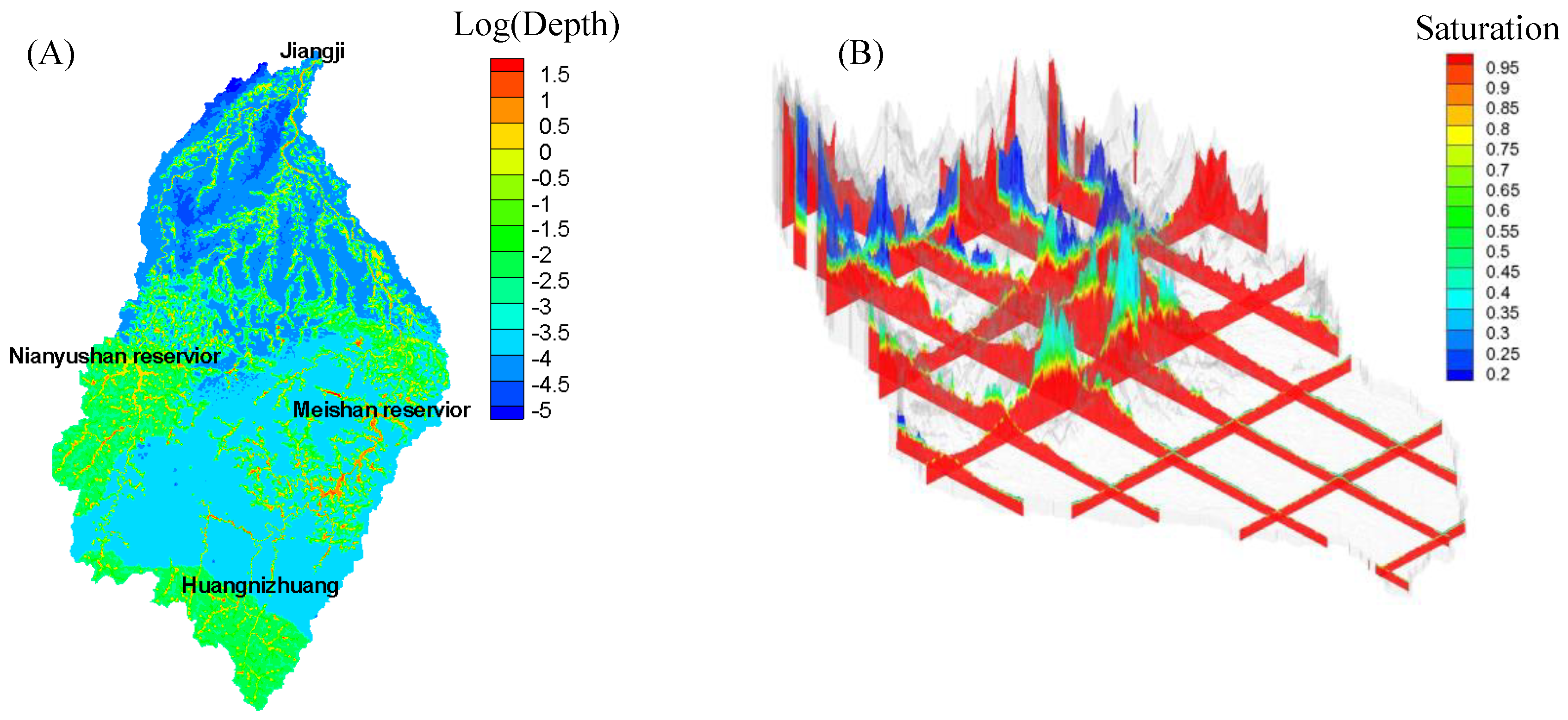
Figure 5A shows the computed steady-state surface water depth, and Figure 5B presents computed steady-state subsurface saturation, with nearly full saturation shown in red. Figure 6A shows the computed steady-state water depths in the surface domain. Similarly, Figure 6B presents the computed steady-state subsurface saturation for the period 1961–1990. The reason that the downstream region of the basin has lower steady-state water depths compared to the upstream region is because the soil depths are different. The locations of the Shi river, Guan river, Nianyushan reservoir, and Meishan reservoir are seen. From Figure 6B, in the downstream lowland region, the water table is shallow while in the upstream mountainous region, the water table is relatively deep. Thus, the simulated results are similar to the actual conditions. These steady-state results were used as the initial condition for the transient simulations.
4.2. Spatial Distribution of a Typical Precipitation
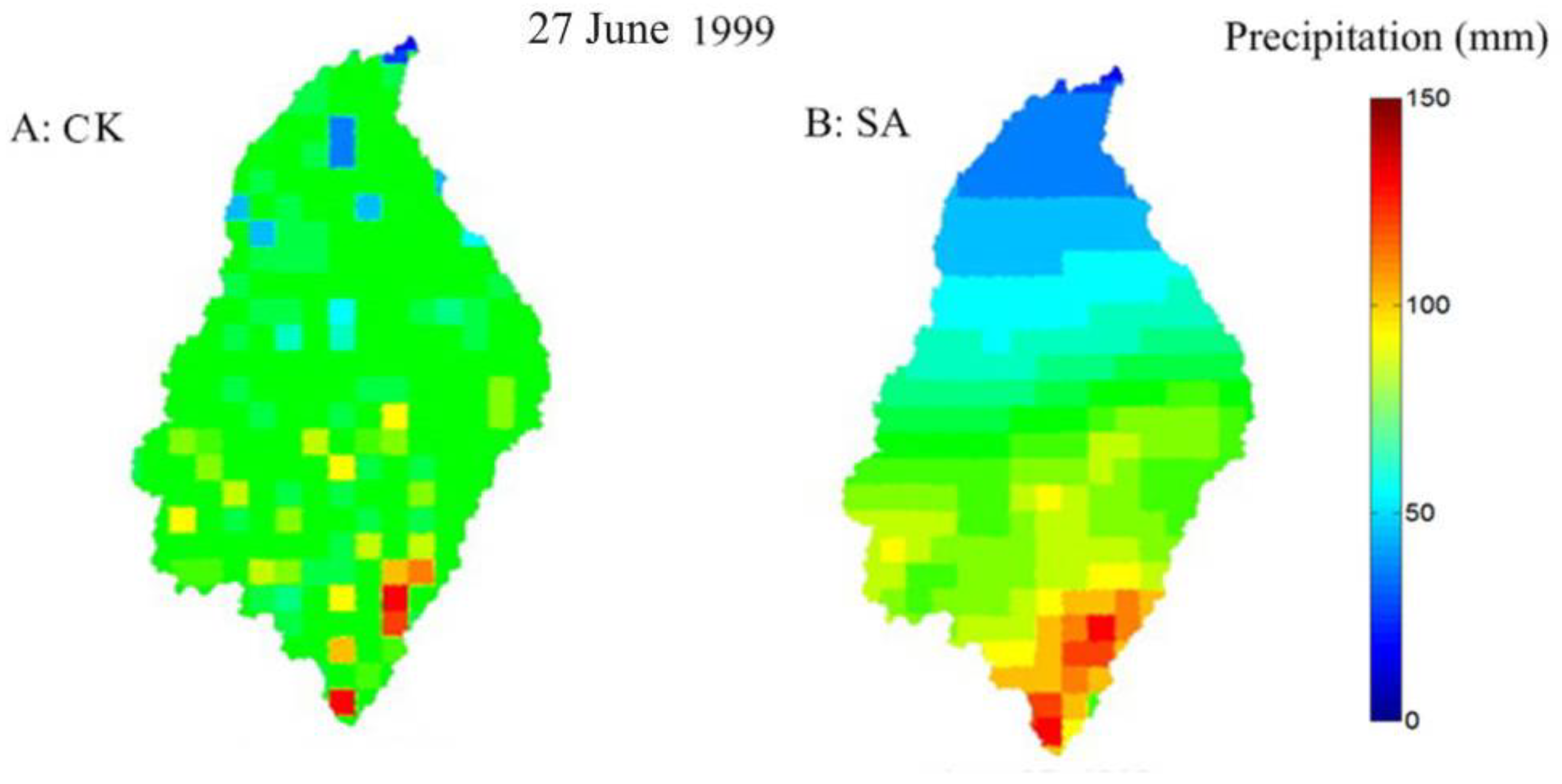
Typical precipitation is employed to explore differences obtained when generating spatial precipitation patterns using TP, CK, and SA. In the simulation period, there is a large precipitation event occurring on 27 June 1999. The results of the statistical analysis for daily precipitation on 27 June 1999, is shown that the mean is 79.55 mm d−1 and the variance is 11,630.69 mm2d−1 between 48 gauging stations. The minimum is 8.5 mm d−1 and the maximum is 167.9 mm d−1. This indicates that the difference in the daily precipitation between the observation points is very high. The daily spatial precipitation data at every grid for this single event was calculated using the TP, CK, and SA methods.
The TP method was applied to the 48 gauging stations within the simulation period to compute the precipitation time series, which was applied equally at each node in the surface flow domain. However, high variance cases such as this example present a difficulty when the TP method is used and can lead to large errors in the precipitation inputs. In this example, using the TP method, the daily precipitation on each grid is the same: 74.5 mm d−1. The different precipitation patterns can be obtained using the CK and SA methods. Figure 6 illustrates these differences. In Figure 6, the spatial resolution is 5 km × 5 km. Figure 6A indicates a region of high precipitation at the southern end of the Shiguan river basin and confirms that the CK method tends to smooth extreme values of the precipitation data set. Although they exhibit the general spatial patterns of the precipitation distribution, the CK method may overestimate the size of areas of high and low precipitation.
For the SA method, some parameters need to be selected. After many experiments, the best parameters with the smallest variance were obtained. R = 0.001; Tf = 0.0001; N = 10,000; K = 106. Then SA model was run 10 times. If the variance and the average value have little difference between differential times, then a stable status is reached. The corresponding weight is the required weight. The above-mentioned hour-scale precipitation data was obtained using the interpolation method. Then the hour-scale precipitation data were merged to obtain daily precipitation data. Figure 6B shows the spatial distribution of precipitation data obtained by averaging 10 SA simulations on 27 June 1999.
The stochastic simulation seeks to minimize a local error variance and focuses on the reproduction of the sample histogram and the semivariogram model (objective function) in addition to honoring the data values [21]. The simulated maps of the precipitation appear to be more realistic than those obtained with the CK method because they reproduce the spatial variability from the sample information. The simulated maps reveal that the spatial distribution and 10 simulated SA realizations preserve the spatial variation of the measured field, such as the delineation of the high and low precipitation areas.
The TP method does not reflect the effect of elevation on precipitation. The CK method uses elevation information. The effect of elevation can be eliminated. However, the weights have a large effect on the CK method. It does not accurately describe the spatial distribution of precipitation. SA method is used to accurately invert the spatial distribution of precipitation. SA method can eliminate the effect of elevation.
At large basin scales, the spatial variability of rainfall affects the flooding process. At field scale or hillside scale, spatial precipitation variability is not a major factor in runoff forecasting. For example, in the Shiguan River Basin, the maximum rain appeared at 3:00 p.m., 27 June 1999, and it was 500 km away from Jiangji hydrology Station. The peak time of the flood peak was 9:00 p.m., 27 June 1999.
4.3. Transient Simulations
4.3.1. Large-Scale Simulated Streamflow Results
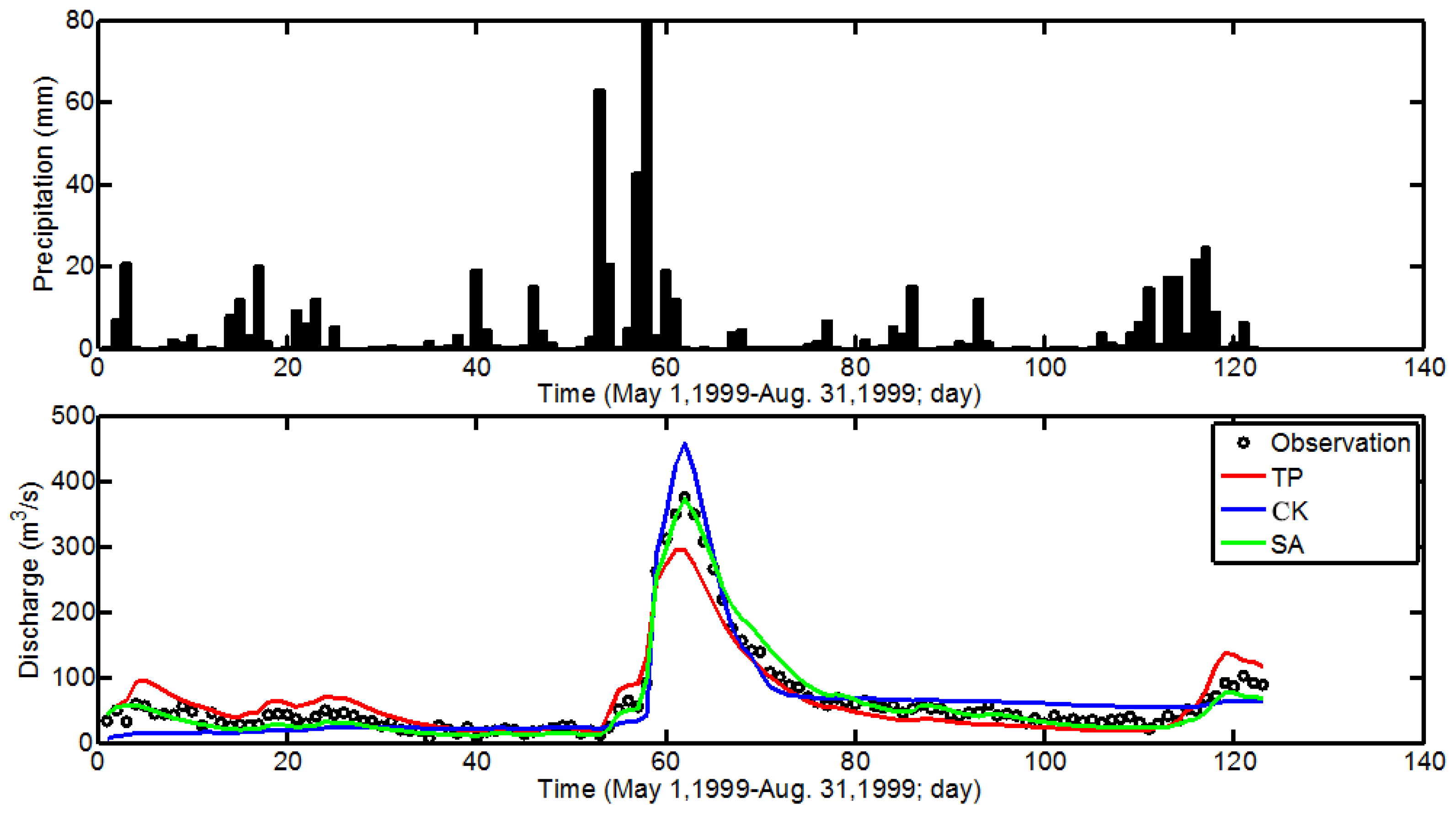
Figure 7 shows the simulated streamflow computed by the HGS hydrology model driven by the TP, CK, and SA precipitation data. The input data (precipitation) was a daily scale and the output data (streamflow) was the daily scale. The simulation period was between 1 May 1999, and 31 August 1999. For the SA method, SA was run 10 times, the daily rainfall at each grid point could be obtained during the simulation period. A random simulation can be performed for the precipitation at each grid point. After comparison, the 10 SA simulation results were not very different in space. Table 5 shows the statistical analysis of 10 spatial precipitation simulations on 27 June 1999 in the Shiguan Basin and the Huangnizhuang basin using SA method. The simulated maximum precipitation location is on the same grid, and the variance of the 10 simulations is also small in Huangnizhuang basin. The daily precipitation was obtained from the average of the 10 simulations to overcome the random error at each grid during the simulation period. The data were used to drive the HGS model. The simulated results driven by three different precipitation data are shown in Figure 7 and Figure 8.
Our study found that the TP method underestimates the streamflows and the CK method overestimates the streamflows at Jiangji hydrological station, while the results of the two methods are opposite at the Huangnizhuang hydrological station. However, the SA case was slightly more accurate than the other two cases. For flood forecasting, the time of the flood peak and the value of flood peak are most important. Driving the HGS model using TP precipitation data, the peak is often underestimated. This is because TP case uses a precipitation average over a large scale and the spatial precipitation data are calculated using a simple method. As such, TP-data are not suitable for use with the HGS hydrology model for flood forecasts. The SA-data and CK-data can, however, be used to drive the HGS model to simulate the peak flow time and peak values. There were eight days during which the observed runoff is between 200 and 400 m3/s. The TP case underestimated the peak streamflow, where the CK cases slightly overestimated the peak flow. The reason for the overestimation was because of the spatial differences in the rainfall patterns. The flood peak arrived too early and the flood waters recede too late. However the SA case caught the peak value of the flood. For the other days, the precipitation was small, the runoff was small and most of the discharge was less than 100 m3/s. The simulated streamflow was most accurate for three cases.
From the statistical analysis, Nash–Sutcliffe efficiency (NSE) was 0.95 for the SA case, 0.82 for the CK case, and 0.8 for the TP method. For NSE, the larger values in a time series were strongly overestimated whereas lower values were neglected, so this led to an overestimation of the model performance during peak flows and an underestimation during low flow conditions. NSE was different in the three cases. The SA method was suitable for catching flood peaks. R also supports this result. R was 0.98 for SA case and 0.95 for CK case and 0.90 for TP case. The RMSE for SA case was the lowest among the three cases. Because the watershed area was large and there were two large reservoirs in the basin, the simulation results were impacted. This results in NSE, R, and RMSE were not satisfied. However for the three cases, the simulated total water resources amount is the same and only the distribution of the streamflow was differential, so the precipitation spatial variable had a large impact on the simulated streamflow. Thus, for assessing water resources in a large-scale system, the use of CK data may be sufficient. If the HGS model is employed to forecast flooding, the use of SA or CK interpolated precipitation data is adequate and SA the case is more accurate.
4.3.2. Medium-Scale Simulated Streamflow Results
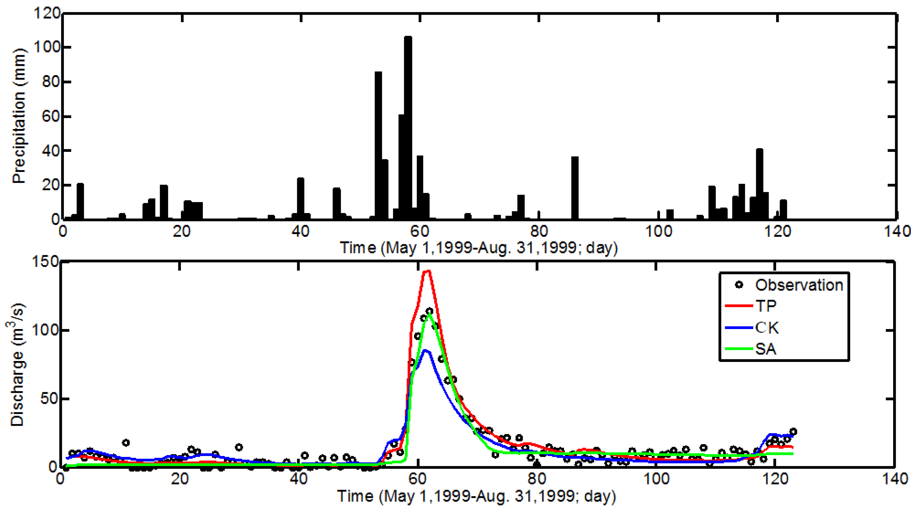
In this section, we only consider the region of the Shiguan river basin that is upstream of the Huangnizhuang hydrology station. This is a medium-scale watershed which is about one seventh the size of the large-scale model and contains only 10 of the original 48 observation points, to which we apply the same methods as we did previously to compute the precipitation distribution for the three rainfall distribution methods (TP, CK, and SA). Our purpose here is not to analyze the differences in the resulting precipitation distribution, but to focus instead on the simulated streamflow at the Huangnizhuang hydrology station, which is shown in Figure 8 for the three cases (TP, CK, and SA). Because the watershed is medium scale, the simulated results for the three cases were all better than those for the large-scale simulation. The NSE and R-values were larger than those obtained for the large-scale simulation. The lowest R was the TP case at 0.96. The lowest NSE was the TP case too at 0.96.
The simulated streamflows were very accurate for three cases. For two large flood peaks (>100 m3/s), the observed streamflow was overestimated for the TP case. The reason for overestimating was because the forcing precipitation data are the surface average and therefore could not capture accurately the information of the distribution of the precipitation. For the CK case, the streamflow was underestimated. This was because the gridded CK precipitation data underestimated the actual maximum precipitation location and overestimated the minimum precipitation zone. The SA method was the best among the three cases and the RMSE of the SA case was the lowest among the three cases.
There were six days in which the observed streamflow was between 50 and 100 m3/s. For the TP case, the streamflow was overestimated. The reasons were that (1) the spatial differences for the precipitation were relatively large; and (2) for physically based surface-subsurface hydrological models, the spatially gridded precipitation data had a large impact on the simulated results. If the observed streamflow was less than 50 m3/s, there was no clear difference between the simulation results and the observed data between all three of the cases. The CK data and SA data generally reflect the spatial variations of the rainfall, and the use of more than one method to estimate the gridded precipitation data may be more suitable to force distributed hydrological models.
In summary, the TP average precipitation may be used to drive a fully integrated distributed hydrology model when the area is small, but its use is not suitable if the area is large. The simulation results obtained using the CK and SA interpolated precipitation data are more satisfactory than those for the TP case. The SA case can capture both the magnitude and timing of flood peaks.
5. Summary and Conclusions
The physically based, fully-integrated, surface-subsurface hydrological model HGS was used to simulate the rainfall-runoff response within the Shiguan river watershed, China, (large-scale) and the Huangnizhuang watershed (medium-scale) during the period 1 May 1999 and 31 August 1999. The primary objective was to assess the runoff response of the integrated hydrological model when driven by different algorithms to infer the spatial precipitation patterns. Here, three methods were used to produce the precipitation patterns: the TP, CK, and SA methods.
First, the hydrological model was calibrated to obtain some key hydrological/hydrogeological parameters and to establish an appropriate initial condition. This initial condition was obtained by spinning up the HGS model to a steady-state equilibrium condition for the coupled surface-subsurface system constrained by the annual-average streamflow rates at five gauging stations distributed over the entire surface of the watershed, as well as by thirty years of hydraulic head data representing the long-term watertable elevation within the watershed. The level of agreement between the simulated and measured hydraulic heads and drainage network patterns indicated that the steady-state model reasonably captured the essence of the surface and subsurface hydraulic characteristics of the watershed. It is reasonable to assume that the steady-state results can be used as the initial condition for the transient simulations. Most of the model parameters were obtained from the literature, with some parameter adjustment during model calibration.
The TP method computes the spatial average value of precipitation for the entire region, which was applied equally at every land surface node in the finite element mesh. The CK and SA methods yielded the spatial distribution of the precipitation such that each mesh node on the land surface could have different values. The CK methods tended to overestimate the regions of low precipitation and underestimate the high values, so the largest flood peak was underestimated for the CK method. The TP methods tended to overestimate the regions of large precipitation and underestimate the regions of the low precipitation, so the largest flood was overestimated for the TP method.
For the large-scale watershed, the flood peak was not captured for the TP and CK cases. The CK case underestimated the flood peak, the TP case overestimated the flood peak, but the SA case accurately simulated the flood peak. Two dams exist in this watershed where the discharge is artificially controlled. Nevertheless, the CK case and SA case were still somewhat better than the TP case.
For the medium-scale watershed, the HGS model was able to capture the flood peak, but it was slightly underestimated for the CK case. For the TP- and SA cases, HGS could adequately capture the flood peak, and the simulated flood peak for the SA case was the best among the three cases.
The spatial rainfall variability at larger catchment scales has a large impact on the accuracy of the rainfall-runoff process simulation. Due to the lack of existing observational data, it is impossible to deeply investigate and accurately describe the scale dependence of the impact of rainfall changes on the rainfall runoff process. Clearly, on a plot or hillslope scale, spatial rainfall variability is not a major concern for discharge prediction (provided rainfall is measured locally). On the scale of a large river basin, local rainfall extremes may not be as important as getting the correct overall trend (along with the questions of flood routing, etc.). The results in this paper cannot explain the scale dependency.
The spatial variability on the small scale is not very large. For the hydrological process simulation, the simplest TP method can be used to obtain the average value of surface precipitation as the driving data of the hydrological model. If the watershed scale is large, the spatial variability of precipitation is large too. Some appropriate methods, such as the SA method, can be chosen to find the accurate precipitation at each grid. The simulated rainfall-runoff process will be more accurate.
At large basin scales, obtaining an accurate flood process is very important. The SA method combined with a distributed hydrological model can obtain an accurate flood process.
The study demonstrated that a physically based, fully-integrated surface-subsurface hydrologic model (HGS) can be employed to simulate the rainfall-runoff response in a watershed of large areal extent provided it is driven by a proper depiction of the spatial pattern of the precipitation that drives it. In summary, it was found that the spatially distributed precipitation data obtained with the SA method is better suited for representing the precipitation patterns than the other two methods used here, and when used to drive the HGS model, very reasonable flood forecasting could be performed.
Calibration is based on PDE-based hydrological process simulation. This model can not only simulate a single runoff process but also be used to study the spatial distribution of precipitation, the relationship between rainfall intensity and runoff, such as where the extreme runoff comes from, the contribution of groundwater, etc. Because of the lack of isotope observations and groundwater level data, these problems have not been studied in this paper. In the future, more detailed studies can be conducted. Furthermore, under different frameworks of interpolation methods, the obtained results are expected to use for optimal parallel runoff-related drought analysis by calculating SRI and to improve the knowledge of drought status.
Author Contributions
Conceptualization, H.L. and Q.W.; methodology, Q.W.; software, Q.W.; validation, H.L. and Q.W.; formal analysis, Q.W. and Y.Z.; writing—review and editing, R.H.; supervision, R.H. All authors have read and agreed to the published version of the manuscript.
Funding
This research is funded by National Key Research and Development Program (grant number: 2019YFC1510504); NNSF (grant numbers: 41830752, 41961134003, 42071033).
Institutional Review Board Statement
Not applicable.
Informed Consent Statement
Not applicable.
Data Availability Statement
The Hydrological monitoring data are provided by the Information center of the Chinese Ministry of Water Resources (http://xxzx.mwr.gov.cn/, accessed on 28 May 2021), The China regional soil type classification database is accessed from the Institute of Soil Science, CAS (http://vdb3.soil.csdb.cn/, accessed on 28 May 2021), The China regional hydrogeology classification database is obtained from the Ministry of Geology and Mineral Resources of P.R. China (http://www.ngac.cn/, accessed on 28 May 2021), DEM are from the ASTER Global Digital Elevation Map (https://asterweb.jpl.nasa.gov/gdem.asp, accessed on 28 May 2021), 1-km Global Land Cover Classification data are provided by The University of Maryland (https://www.earthenv.org/landcover, accessed on 28 May 2021).
Conflicts of Interest
The authors declare no conflict of interest.
References
- Van Huijgevoort, M.H.J.; Hazenberg, P.; Van Lanen, H.A.J.; Teuling, A.J.; Clark, D.B.; Folwell, S.; Gosling, S.N.; Hanasaki, N.; Heinke, J.; Koirala, S.; et al. Global Multimodel Analysis of Drought in Runoff for the Second Half of the Twentieth Century. J. Hydrometeorol. 2013, 14, 1535–1552. [Google Scholar] [CrossRef] [Green Version]
- Shukla, S.; Wood, A.W. Use of a standardized runoff index for characterizing hydrologic drought. Geophys. Res. Lett. 2008, 35. [Google Scholar] [CrossRef] [Green Version]
- Freeze, R.; Harlan, R. Blueprint for a physically-based, digitally-simulated hydrologic response model. J. Hydrol. 1969, 9, 237–258. [Google Scholar] [CrossRef]
- Vander-Kwaak, J.E.; Loague, K. Hydrologic-Response simulations for the R-5 catchment with a comprehensive physics-based model. Water Resour. Res. 2001, 37, 999–1013. [Google Scholar] [CrossRef]
- HydroGeologic-Inc. A MODFLOW-Based Hydrologic Modelling System; HydroGeoLogic Inc.: Herndon, VA, USA, 2001. [Google Scholar]
- Panday, S.; Huyakorn, P.S. A fully coupled physically-based spatially-distributed model for evaluating surface/subsurface flow. Adv. Water Resour. 2004, 27, 361–382. [Google Scholar] [CrossRef]
- Aquanty-Inc. HydroGeoSphere User Guide; Aquanty Inc.: Waterloo, ON, Canada, 2013. [Google Scholar]
- Abdelghani, F.B.; Aubertin, M.; Simon, R.; Therrien, R. Numerical simulations of water flow and contaminants transport near mining wastes disposed in a fractured rock mass. Int. J. Min. Sci. Technol. 2015, 25, 37–45. [Google Scholar] [CrossRef]
- Loague, K.; Vander-Kwaak, J.E. Simulating hydrological response for the R-5 catchment: Comparison of two models and the impact of the roads. Hydrol. Process. 2002, 16, 1015–1032. [Google Scholar] [CrossRef]
- Pebesma, E.J.; Paul, S.; Keith, L. Error analysis for the evaluation of model performance: Rainfall–runoff event time series data. Hydrol. Process. 2005, 19, 1529–1548. [Google Scholar] [CrossRef]
- Heppner, C.S.; Ran, Q.; VanderKwaak, J.E.; Loague, K. Adding sediment transport to the integrated hydrology model (InHM): Development and testing. Adv. Water Resour. 2006, 29, 930–943. [Google Scholar] [CrossRef]
- Shrestha, R.; Tachikawa, Y.; Takara, K. Input data resolution analysis for distributed hydrological modeling. J. Hydrol. 2006, 319, 36–50. [Google Scholar] [CrossRef]
- Refsgaard, J.C.; Højberg, A.L.; Møller, I.; Hansen, M.; Søndergaard, V. Groundwater Modeling in Integrated Water Resources Management-Visions for 2020. Ground Water 2010, 48, 633–648. [Google Scholar] [CrossRef]
- Lindström, G.; Johansson, B.; Persson, M.; Gardelin, M.; Bergström, S. Development and test of the distributed HBV-96 hydrological model. J. Hydrol. 1997, 201, 272–288. [Google Scholar] [CrossRef]
- Li, Q.; Unger, A.; Sudicky, E.; Kassenaar, D.; Wexler, E.; Shikaze, S. Simulating the multi-seasonal response of a large-scale watershed with a 3D physically-based hydrologic model. J. Hydrol. 2008, 357, 317–336. [Google Scholar] [CrossRef]
- Jones, J.P.; Sudicky, E.A.; McLaren, R.G. Application of a fully-integrated surface-subsurface flow model at the watershed-scale: A case study. Water Resour. Res. 2008, 44, 893–897. [Google Scholar] [CrossRef]
- Goderniaux, P.; Brouyère, S.; Fowler, H.J.; Blenkinsop, S.; Therrien, R.; Orban, P.; Dassargues, A. Large scale surface-subsurface hydrological model to assess climate change impacts on groundwater reserves. J. Hydrol. 2009, 373, 122–138. [Google Scholar] [CrossRef]
- Krysanova, V.; Müller-Wohlfeil, D.-I.; Becker, A. Development and test of a spatially distributed hydrological/water quality model for mesoscale watersheds. Ecol. Model. 1998, 106, 261–289. [Google Scholar] [CrossRef]
- Seo, D.-J.; Krajewski, W.F.; Azimi-Zonooz, A.; Bowles, D.S. Stochastic interpolation of rainfall data from rain gages and radar using Cokriging: 2. Results. Water Resour. Res. 1990, 26, 915–924. [Google Scholar] [CrossRef]
- Grimes, D.; Pardo-Iguzquiza, E.; Bonifacio, R. Optimal areal rainfall estimation using raingauges and satellite data. J. Hydrol. 1999, 222, 93–108. [Google Scholar] [CrossRef]
- Goovaerts, P. Geostatistical approaches for incorporating elevation into the spatial interpolation of rainfall. J. Hydrol. 2000, 228, 113–129. [Google Scholar] [CrossRef]
- Bárdossy, A.; Pegram, G.G.S. Copula based multisite model for daily precipitation simulation. Hydrol. Earth Syst. Sci. 2009, 13, 2299–2314. [Google Scholar] [CrossRef] [Green Version]
- Bárdossy, A.; Pegram, G. Interpolation of precipitation under topographic influence at different time scales. Water Resour. Res. 2013, 49, 4545–4565. [Google Scholar] [CrossRef]
- Caruso, C.; Quarta, F. Interpolation methods comparison. Comput. Math. Appl. 1998, 35, 109–126. [Google Scholar] [CrossRef] [Green Version]
- Chen, T.; Ren, L.; Yuan, F.; Yang, X.; Jiang, S.; Tang, T.; Liu, Y.; Zhao, C.; Zhang, L. Comparison of Spatial Interpolation Schemes for Rainfall Data and Application in Hydrological Modeling. Water 2017, 9, 342. [Google Scholar] [CrossRef] [Green Version]
- Greco, A.; De Luca, D.L.; Avolio, E. Heavy Precipitation Systems in Calabria Region (Southern Italy): High-Resolution Observed Rainfall and Large-Scale Atmospheric Pattern Analysis. Water 2020, 12, 1468. [Google Scholar] [CrossRef]
- Kurtzman, D.; Navon, S.; Morin, E. Improving interpolation of daily precipitation for hydrologic modelling: Spatial patterns of preferred interpolators. Hydrol. Process. 2009, 23, 3281–3291. [Google Scholar] [CrossRef]
- Moulin, L.; Gaume, E.; Obled, C. Uncertainties on mean areal precipitation: Assessment and impact on streamflow simulations. Hydrol. Earth Syst. Sci. 2009, 13, 99–114. [Google Scholar] [CrossRef] [Green Version]
- Wilson, C.B.; Valdés, J.B.; Rodriguez-Iturbe, I. On the influence of the spatial distribution of rainfall on storm runoff. Water Resour. Res. 1979, 15, 321–328. [Google Scholar] [CrossRef]
- Vinogradov, N.A.; Schulte, K.; Ng, M.L.; Mikkelsen, A.; Lundgren, E.; Mårtensson, N.; Preobrajenski, A.B. Impact of Atomic Oxygen on the Structure of Graphene Formed on Ir(111) and Pt(111). J. Phys. Chem. C 2011, 115, 9568–9577. [Google Scholar] [CrossRef]
- Ly, S.; Charles, C.; Degre, A. Different methods for spatial interpolation of rainfall data for operational hydrology and hydrological modeling at watershed scale. A review. Biotechnol. Agron. Société Environ. 2013, 17, 392–406. [Google Scholar] [CrossRef]
- Goovaerts, P. Geostatistics for Natural Resources Evaluation. Technometrics 1997, 42, 437–438. [Google Scholar]
- Goovaerts, P. Geostatistical modelling of uncertainty in soil science. Geoderma 2001, 103, 3–26. [Google Scholar] [CrossRef]
- Shrestha, R.; Tachikawa, Y.; Takara, K. Performance analysis of different meteorological data and resolutions using MaScOD hydrological model. Hydrol. Process. 2004, 18, 3169–3187. [Google Scholar] [CrossRef]
- Verseghy, D.L. Class-A Canadian land surface scheme for GCMS. I. Soil model. Int. J. Clim. 2007, 11, 111–133. [Google Scholar] [CrossRef]
- Verseghy, D.L.; McFarlane, N.A.; Lazare, M. Class—A Canadian land surface scheme for GCMS, II. Vegetation model and coupled runs. Int. J. Clim. 1993, 13, 347–370. [Google Scholar] [CrossRef]
- Lin, C.A.; Wen, L.; Lu, G.; Wu, Z.; Zhang, J.; Yang, Y.; Zhu, Y.; Tong, L. Atmospheric-hydrological modeling of severe precipitation and floods in the Huaihe River Basin, China. J. Hydrol. 2006, 330, 249–259. [Google Scholar] [CrossRef]
- Wen, L.; Wu, Z.; Lu, G.; Lin, C.A.; Zhang, J.; Yang, Y. Analysis and improvement of runoff generation in the land surface scheme CLASS and comparison with field measurements from China. J. Hydrol. 2007, 345, 1–15. [Google Scholar] [CrossRef]
- Lin, C.A.; Wen, L.; Lu, G.; Wu, Z.; Zhang, J.; Yang, Y.; Zhu, Y.; Tong, L. Real-time forecast of the 2005 and 2007 summer severe floods in the Huaihe River Basin of China. J. Hydrol. 2010, 381, 33–41. [Google Scholar] [CrossRef]
- Therrien, R.; McLaren, R.G.; Sudicky, E.A.; Panday, S.M. HydroGeoSphere: A Three-Dimensional Numerical Model Describing Fully-integrated Subsurface and Surface Flow and Solute Transport; Groundwater Simulations Group; University of Waterloo: Waterloo, ON, Canada, 2005. [Google Scholar]
- Therrien, R.; Sudicky, E. Three-dimensional analysis of variably-saturated flow and solute transport in discretely-fractured porous media. J. Contam. Hydrol. 1996, 23, 1–44. [Google Scholar] [CrossRef]
- Kristensen, K.J.; Jensen, S.E. A model for estimating actual evapotranspiration from potential evapotranspiration. Hydrol. Res. 1975, 6, 170–188. [Google Scholar] [CrossRef] [Green Version]
- Fu, S.; O Sonnenborg, T.; Jensen, K.H.; He, X. Impact of Precipitation Spatial Resolution on the Hydrological Response of an Integrated Distributed Water Resources Model. Vadose Zone J. 2011, 10, 25–36. [Google Scholar] [CrossRef]
- Journel, A.G.; Huijbregts, C.J. Mining Geostatistics; Academic Press: New York, NY, USA, 1978. [Google Scholar]
- Kirkpatrick, S.; Gelatt, C.D.; Vecchi, M.P. Optimization by Simulated Annealing. Science 1983, 220, 671–680. [Google Scholar] [CrossRef] [PubMed]
- Aziz, M.K.B.M.; Yusof, F.; Daud, Z.M.; Yusop, Z.; Kasno, M.A. Redesigning rain gauges network in johor using geostatistics and simulated annealing. AIP Conf. Proc. 2015, 1643, 270–277. [Google Scholar]
- Vázquez, R. Effect of potential evapotranspiration estimates on effective parameters and performance of the MIKE SHE-code applied to a medium-size catchment. J. Hydrol. 2003, 270, 309–327. [Google Scholar] [CrossRef]
- Schaap, M.G.; Leig, F.J.; Van Genuchten, M.T. Rosetta: A Computer Program for Estimating Soil Hydraulic Properties with Hierarchical Pedotransfer Functions. J. Hydrol. 2001, 251, 163–176. [Google Scholar] [CrossRef]
- Lü, H.; Yu, Z.; Horton, R.; Zhu, Y.; Zhang, J.; Jia, Y.; Yang, C. Effect of Gravel-Sand Mulch on Soil Water and Temperature in the Semiarid Loess Region of Northwest China. J. Hydrol. Eng. 2011, 18, 1484–1494. [Google Scholar] [CrossRef]
- Lü, H.; Yu, Z.; Zhu, Y.; Drake, S.; Hao, Z.; Sudicky, E.A. Dual state-parameter estimation of root zone soil moisture by optimal parameter estimation and extended Kalman filter data assimilation. Adv. Water Resour. 2011, 34, 395–406. [Google Scholar] [CrossRef]
- Duan, Q.; Sorooshian, S.; Gupta, V.K. Optimal use of the SCE-UA global optimization method for calibrating watershed models. J. Hydrol. 1994, 158, 265–284. [Google Scholar] [CrossRef]
- Krause, P.; Boyle, D.P.; Bäse, F. Comparison of different efficiency criteria for hydrological model assessment. Adv. Geosci. 2005, 5, 89–97. [Google Scholar] [CrossRef] [Green Version]
- Lü, H.; Li, X.; Yu, Z.; Horton, R.; Zhu, Y.; Hao, Z.; Xiang, L. Using a H∞ filter assimilation procedure to estimate root zone soil water content. Hydrol. Process. 2010, 24, 3648–3660. [Google Scholar] [CrossRef]
Figure 1.
Location of the Shiguan river basin.

Figure 2.
Land use characteristics, soil types, and hydrogeology types within the Shiguan river basin.
Figure 2.
Land use characteristics, soil types, and hydrogeology types within the Shiguan river basin.

Figure 3.
Spatial discretization of the Shiguan River basin.

Figure 4.
Scheme of solution procedure using SA.

Figure 5.
(A) Computed steady-state surface water depth. (B) Computed steady-state subsurface saturation, with nearly full saturation shown in red.
Figure 5.
(A) Computed steady-state surface water depth. (B) Computed steady-state subsurface saturation, with nearly full saturation shown in red.

Figure 6.
The spatial distribution of precipitation for a large rainfall in the simulation period using CK (A) and SA (B).
Figure 6.
The spatial distribution of precipitation for a large rainfall in the simulation period using CK (A) and SA (B).

Figure 7.
Simulated and observed hydrograph at Jiangji hydrology station.

Figure 8.
Simulated and measured hydrograph at Huangnizhuang hydrology station.


Table 1.
Parameters used in the flow model.
| Subsurface Domain | Meaning | Unit |
|---|---|---|
| Saturated hydraulic conductivity | ||
| Porosity | - | |
| Specific storage | ||
| van Genuchten parameter | - | |
| van Genuchten parameter | ||
| Residual water saturation | - | |
| Surface domain | ||
| Coupling length | L | |
| Manning roughness coefficient | ||
| Manning roughness coefficient | ||
| Evapotranspiration | ||
| Evaporation depth | L | |
| Evaporation limiting saturations | - | |
| Leaf area index | - | |
| Root depth | L | |
| Transpiration fitting parameters | - | |
| Transpiration limiting saturations | - | |
| Canopy storage parameter | L |
Table 2.
Values for the Manning roughness coefficients and coupling length.
| Land Use | ||
|---|---|---|
| m−1/3 d | m | |
| Forest | 0.1 | |
| Agricultural | 0.1 | |
| Bare rock | 0.1 | |
| Urban and rural | 0.1 | |
| Alluvium | 0.1 |
Table 3.
Van Genuchten parameters, total porosity, specific storage and full saturated hydraulic conductivities.
Table 3.
Van Genuchten parameters, total porosity, specific storage and full saturated hydraulic conductivities.
| Layer | Type | K | |||||
|---|---|---|---|---|---|---|---|
| [-] | [d−1] | [-] | [-] | [d−1] | [m d−1] | ||
| Soil | Anthrosols | 0.059 | 1.480 | 0.256 | 0.5 | 0.008 | |
| Luvisols | 0.006 | 1.590 | 0.166 | 0.45 | 0.019 | ||
| Semi-hydromorphic soil | 0.009 | 1.510 | 0.188 | 0.35 | 0.022 | ||
| Entisols | 0.020 | 1.410 | 0.149 | 0.45 | 0.016 | ||
| Rock | Clastic rock | 30.00 | 3.000 | 0.050 | 0.25 | 0.2 | |
| Magatic rock | 30.00 | 3.000 | 0.050 | 0.01 | 8.64 × 10⁻⁸ | ||
| Gravel sand | 0.145 | 2.68 | 0.105 | 0.25 | 864 | ||
| Metamorphic rock | 44.6 | 0.21 | 0.030 | 0.01 | 6.0 |
Table 4.
Evapotranspiration parameters from the literature.
| Forest | Grass | Dryland | Urban and Rural | Beach | |
|---|---|---|---|---|---|
| Evaporation depth [m] | 2.0 | 2.0 | 2.0 | 2.0 | 2.0 |
| Root depth () [m] | 5.2 | 2.6 | 0.0 | 0.0 | 0.0 |
| 5.12 | 2.5 | 0.0 | 0.40 | 0.0 | |
| 0.3 | 0.3 | 0.3 | 0.3 | 0.3 | |
| 0.2 | 0.2 | 0.2 | 0.2 | 0.2 | |
| 1 | 1 | 1 | 1 | 1 | |
Table 5.
Statistical analysis of 10 spatial precipitation simulations in the Shiguan Basin and the Huangnizhuang basin using the SA method.
Table 5.
Statistical analysis of 10 spatial precipitation simulations in the Shiguan Basin and the Huangnizhuang basin using the SA method.
| Shiguan | Huangnizhuang | |||||
|---|---|---|---|---|---|---|
| SA Cases | Max | Min | Var | Max | Min | Var |
| 1 | 190.78 | 9.66 | 25.51 | 91.40 | 38.13 | 18.55 |
| 2 | 151.40 | 7.66 | 20.25 | 93.79 | 39.12 | 19.04 |
| 3 | 189.01 | 9.57 | 25.28 | 120.86 | 50.42 | 24.53 |
| 4 | 150.68 | 7.63 | 20.15 | 84.94 | 35.43 | 17.24 |
| 5 | 196.73 | 9.96 | 26.31 | 104.25 | 43.49 | 21.16 |
| 6 | 157.82 | 7.99 | 21.11 | 90.77 | 37.87 | 18.42 |
| 7 | 147.52 | 7.47 | 19.73 | 124.72 | 52.03 | 25.32 |
| 8 | 151.18 | 7.65 | 20.22 | 113.58 | 47.38 | 23.05 |
| 9 | 175.69 | 8.89 | 23.50 | 104.70 | 43.68 | 21.25 |
| 10 | 166.11 | 8.41 | 22.21 | 103.47 | 43.16 | 21.00 |
Publisher’s Note: MDPI stays neutral with regard to jurisdictional claims in published maps and institutional affiliations. |
© 2021 by the authors. Licensee MDPI, Basel, Switzerland. This article is an open access article distributed under the terms and conditions of the Creative Commons Attribution (CC BY) license (https://creativecommons.org/licenses/by/4.0/).
Share and Cite
MDPI and ACS Style
Lü, H.; Wang, Q.; Horton, R.; Zhu, Y. The Response of the HydroGeoSphere Model to Alternative Spatial Precipitation Simulation Methods. Water 2021, 13, 1891. https://doi.org/10.3390/w13141891
AMA Style
Lü H, Wang Q, Horton R, Zhu Y. The Response of the HydroGeoSphere Model to Alternative Spatial Precipitation Simulation Methods. Water. 2021; 13(14):1891. https://doi.org/10.3390/w13141891
Chicago/Turabian StyleLü, Haishen, Qimeng Wang, Robert Horton, and Yonghua Zhu. 2021. "The Response of the HydroGeoSphere Model to Alternative Spatial Precipitation Simulation Methods" Water 13, no. 14: 1891. https://doi.org/10.3390/w13141891
Note that from the first issue of 2016, this journal uses article numbers instead of page numbers. See further details here.