
Possibilities of Using Neuro-Fuzzy Models for Post-Processing of Hydrological Forecasts


1
Czech Hydrometeorological Institute, Kroftova 43, 616 00 Brno, Czech Republic
2
Faculty of Civil Engineering, Institute of Landscape Water Management, Brno University of Technology, Veveří 331/95, 602 00 Brno, Czech Republic
3
Czech Hydrometeorological Institute, A. Staška 1177, Rožnov, 370 07 České Budějovice, Czech Republic
*
Author to whom correspondence should be addressed.
Water 2021, 13(14), 1894; https://doi.org/10.3390/w13141894
Submission received: 11 June 2021
/
Revised: 29 June 2021
/
Accepted: 6 July 2021
/
Published: 8 July 2021
Abstract
:When issuing hydrological forecasts and warnings for individual profiles, the aim is to achieve the best possible results. Hydrological forecasts themselves are burdened by an error (uncertainty) at the inputs (precipitation forecast) as well as on the side of the hydrological model used. The aim of the method described in this article is to reduce the error of the hydrological model using post-processing the model results. Models based on neuro-fuzzy models were selected for the post-processing itself. The whole method was tested on 12 profiles in the Czech Republic. The catchment size of the individual profiles ranged from 90 to 4500 km2 and the profiles varied in their character, both in terms of elevation as well as land cover. After finding the suitable model architecture and introducing supporting algorithms, there was an improvement in the results for the individual profiles for selected criteria by on average 5–60% (relative culmination error, mean square error) compared to the results of re-simulation of the hydrological model. The results of the application show that the method was able to improve the accuracy of hydrological forecasts and thus could contribute to better management of flood situations.
1. Introduction
Short-term hydrological forecasts are an essential part of many early warning systems today. Based on the forecast, it is possible to adjust the management of reservoirs or start preparatory measures against floods. The problem of hydrological forecasts is their accuracy. The forecast itself is affected by uncertainties both on the input side (precipitation, river basin saturation, etc.) and on the hydrological model side (schematization and calibration of the model). The errors caused by the above-mentioned uncertainties are partly systematic (repeated). They can be identified, but often cannot be removed by modifying the hydrological model, because the model cannot capture the whole complexity of the runoff process [1]. However, these errors can be eliminated by one of the methods of adjusting the resulting forecasts—in so-called post-processing. For the above reason, post-processing is commonly introduced in predictions to reduce prediction error.
In practice, commonly used post-processing methods usually only deal with the error associated with the precipitation amount or with hydrological uncertainty, but only with stochastic (ensemble) prediction [2,3,4,5]. Other methods that work directly with the hydrological model error work on the basis of daily flows [6] or longer time periods. In the case of other methods such as the Kalman filter [7], the methods are usually limited to repeated correction of the first value and subsequent adjustment of the prediction (shift of values by the magnitude of the error, time shift). The problem with their use is that the effect of adjusting the first value decreases with increasing time. In addition, repeated recalculations of the model are very time consuming. In the case of the Czech Republic, the forecast length of 72 h is usually used (Czech Hydrometeorological Institute, CHMI). For this reason, a method was developed that is able to correct the error of the hydrological model during a time period of 72 h or more in advance and does not need recalculation (recalibration).
One of the possibilities of post-processing the outputs of the hydrological model are trained neuro-fuzzy models [8]. Trained neuro-fuzzy models are an adaptive-network-based fuzzy inference systems (ANFIS). The advantage of ANFIS is the fact that it represents a combination of neural networks and a fuzzy set, which ANFIS gives certain advantage over classic neural network or trained fuzzy models. For further understanding of ANFIS we recommend a scientific paper of the authors Jang and Sun [8]. The further described model is based on this theory. The advantage of the above models is their calculation speed and the ability to approximate even very complex relationships between the individual factors influencing the resulting course of hydrological forecast. The artificial intelligence methods themselves are very often used for flood flow forecast or reservoir management [9,10,11,12]. Usage of ANFIS as the post-processing method is what makes this study unique. The aim of the method described in this paper is to be able to apply a model, based on the ANFIS method, for post-processing and it is therefore assumed that the reader has certain understanding of the ANFIS method.
The ANFIS itself could be used for flood flow forecasting, but this application has some restrictions and usually has a high demand on sufficient training episodes. The major issue associated with a direct application is related to extrapolation (when forecasted episodes are outside of the training data matrix). The second problem is that a flood is a continuous curve, values of which usually do not differ from hour to hour by a certain difference (results stability problems). The AI method can give rather fluctuating values, without another algorithm. These problems are solved by using a hydrological model. The ANFIS is used for post-processing of hydrological model results to enhance their accuracy. Moreover, the ANFIS is also intended to be used in flood situations only (when it makes sense to apply the post-processing). The hydrological model forecast is provided on a daily basis even when flow values are low (drought forecast).
The uncertainty of hydrological modeling is caused, among other things, by the simplification of reality on a spatial scale (homogenization of river basins into modeled areas) and on a time scale (same set of parameters for different runoff phases). It can be assumed that for a specific river basin, this part of the uncertainty of hydrological modeling will manifest itself by systematic errors, which are repeated in similar runoff situations. The magnitude of these biases depends on many factors such as saturation, initial flow, precipitation, season and others. Therefore, a simple mathematical relationship cannot be established for them. However, trained neuro-fuzzy models can identify (evaluate) these relationships and use them to make the forecast more accurate.
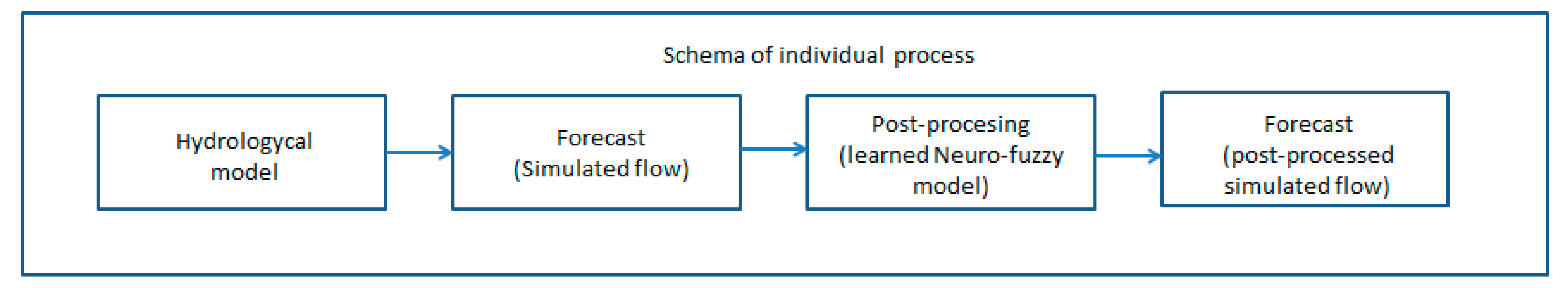
The aim of the described post-processing models based on trained neuro-fuzzy models is to reduce the error of the outputs from the hydrological model for events that were caused by rainfall. In the following text, hydrological forecast will be understood as the deterministic forecast obtained by the continuous hydrological model for gauged (forecasting) profile. The presented method focuses on runoff situations in which there is a risk of floods and thus a considerable pressure to provide the greatest possible reliability of flow forecasts. At the same time, however, we have to emphasize that the method does not solve the errors caused by inaccurate predictions of precipitation, which are often the dominant source of errors during floods. Figure 1 shows a flowchart for the process and also shows where the post-processing stage comes into play during this process.
2. Materials and Methods
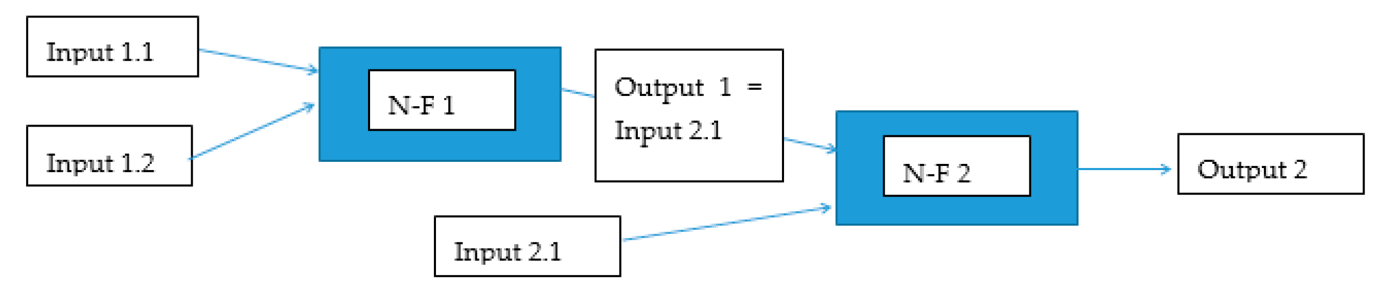
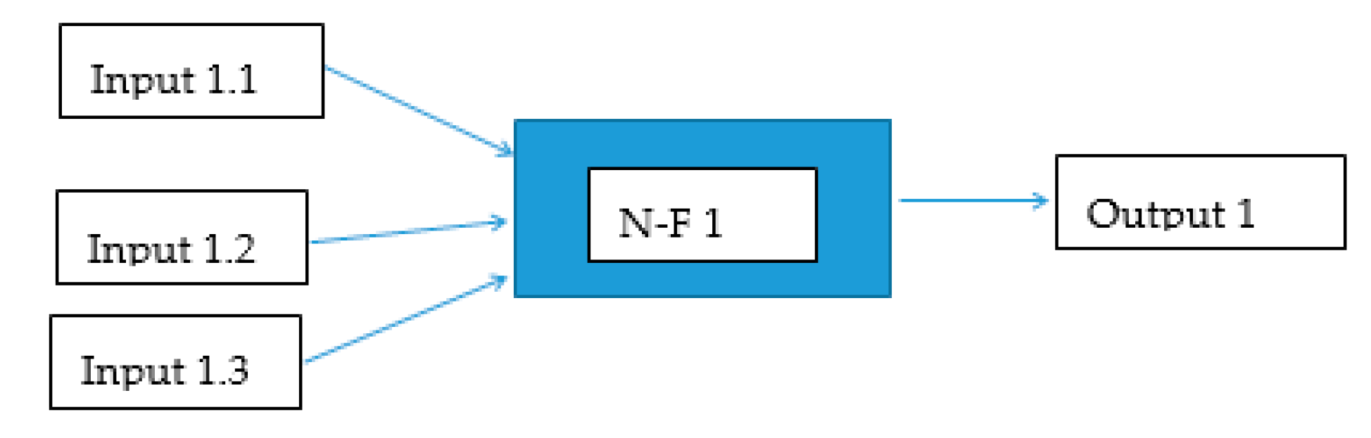
It is, therefore, clear from the previous text that the use of neuro-fuzzy models as a post-processing tool could bring the desired improvement of the existing hydrological forecast methods since the model itself, based on artificial intelligence methods, will be able to mitigate the prediction error. In the model architecture of the trained neuro-fuzzy model NFM, sequential aggregation of inputs was used [13] if the model used 3 or more inputs (Figure 2). Figure 3 depicts the model scheme without sequential aggregation of inputs. The advantage of a gradual aggregation of inputs is easier construction of the rule matrix. First, it is necessary to build a model architecture and a matrix of target behavior containing input-output relationships, because models based on artificial intelligence methods need patterns for their training (learning). Table 1 below lists the individual inputs that were used to find a suitable post-processing model architecture. All flow values are modeled flows by the hydrological model, unless stated otherwise for the flow parameter.
3. Application
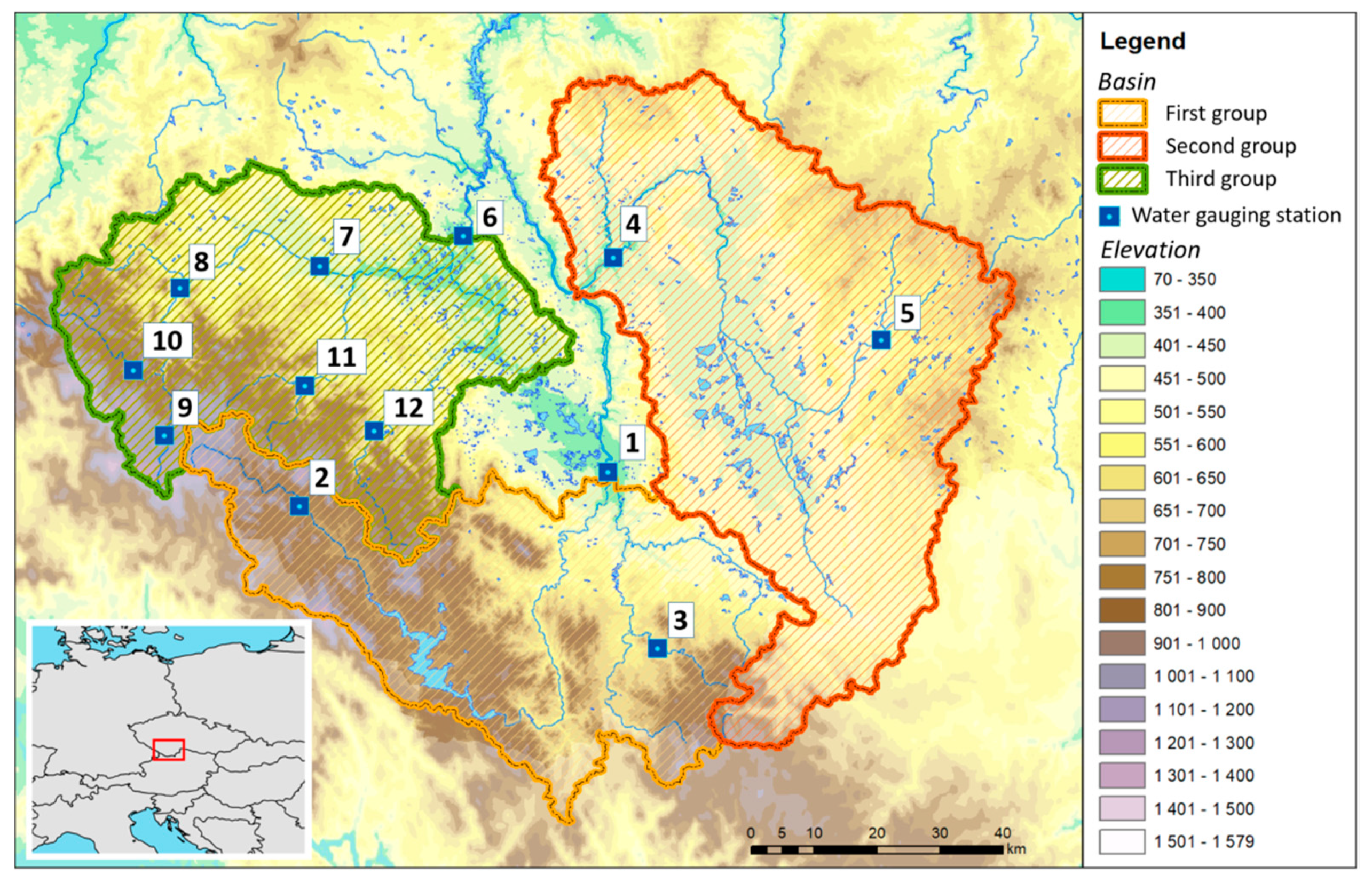
The model described in the previous chapter was applied to selected prediction profiles to test the possibilities of post-processing under various conditions. The area of interest was chosen because there are very diverse types of river basins. There are typical mountain catchments and catchments strongly influenced by agricultural activity as well as catchments with a high proportion of water areas. The profiles themselves were selected from a set of forecasting profiles included in the national flood forecasting service performed by the Czech Hydrometeorological Institute (CHMI). All the selected profiles are located within the Vltava river basin in the Czech Republic in the region of south Bohemia. Their positions are shown in Figure 4 and their brief description is given in Table 2. A total of 12 profiles were selected, which were divided into three groups according to their location. At the end of each profile name, a number is given in parentheses, which represents the position of the profile in Figure 3. The first group consists of the catchments of the Lenora (2), Ličov (3) and České Budějovice (1) profiles. The profile of České Budějovice is in this application the final profile of the whole first group and the area of its catchment area represents the whole area of the catchment area of the first group. The catchments of the Ličov and Lenora profiles are then sub-catchments. The basin of the Ličov and Lenora profiles mostly consists of forests and mountains. The profile of Lenor itself lies above the Lipno reservoir. The second group consists of the profiles Bechyně (4) and Rodvínov (5). The Bechyně profile is the final profile of the whole group. The Bechyně profile catchment area and its partial part of the Rodvínov catchment area are relatively flat with a large percentage of agricultural land and include a large number of ponds and pond systems (5.1% of the catchment area). The third group consists of the profiles Bohumilice (11), Katowice (7), Modrava (9), Písek (6), Podedvory (12), Stodůlky (10) and Sušice (8). The Písek profile is the final profile of the entire third group. The catchment area of the Bohumilice, Modrava, Stodůlky and Sušice profiles is mainly made up of forests. The catchments of the Bohumilice, Modrava and Stodůlky profiles themselves have a mountain character.
Table 2 shows the catchment area and the average long-term flow Qa. Furthermore, for the individual profiles, values of flows are given, at which the individual degrees of flood activity are announced, which are defined by the Water Act of the Czech Republic 254/2001 of the Collection of Laws. The values of the flood level danger (FLD) levels themselves represent the individual limit values for the declaration of a flood danger (FLD 1—low level of danger—yellow color; FLD 2—high level of danger-orange color; FLD 3—extreme level of danger—red color). The particular level of danger usually corresponds with this color set in a global warning system. The individual values of flows in the FLD columns were determined according to the measurement curve valid at the time of validation of the post-processing model. Column N1 shows the one-year flood flow rate value and column N100 shows the 100-year flood flow rate value. The last column of the table shows the percentage of forest area with respect to the total catchment area FIP. The FIP parameter is used for better understanding of the basin.
Input data of model flow, soil saturation and average precipitation data for each river basin were obtained by using the Aqualog [14] hydrological model, which is used in this part of the river basin for operational calculation of the hydrological forecast. The Aqualog is a hydrological modeling system that integrates the rainfall-runoff model Sacramento (SAC-SMA) [15], the snow accumulation and melting model Snow17 [16] and the channel routing model TDR [17]. The spatial structure of modeling techniques is semi-distributed with an average area of the catchments between 30 and 50 km2. The required inputs are data on river discharge, precipitation and air temperature in 1-h step. The precipitation data, which were used for resimulation, were merged with rainfall data (combination of adjusted radar observation and values measured by automatic weather station). Aqualog re-simulation data were calculated on the observed data in continuous intervention-free operation. Deviations of the calculated flow from the observed values therefore represent the error of the input observed data and hydrological modeling. The re-simulation period 2005–2016 includes a number of significant flood episodes. The data were grouped into individual months and the tendency of the simulation model compared to the reality in the individual months was determined. Data from a particular month were selected for the training of the model for the that particular month, and if the neighboring months had the same tendency (underestimated, overestimated), the training matrix was extended by these data. Data of distant months were not considered, even if they had the same tendency. The reason for this selection was the time variability of the influence of the model sensitivity on the individual input parameters of the simulation model and the variable boundary conditions of the simulation model. Data from neighboring months that met the condition of the same tendency were included only due to the lack of training data during the individual months.
During the calibration process, optimal settings and architecture of the individual models were sought. For the NFM model, it was the shape number of membership functions further marked mf and sequence of input. The calibration period was chosen from 2005 to 2010 and was gradually extended by new (past) events. Individual events were selected for the calibration process on the basis of their peak flow and total precipitation Hs. The event started when the hourly precipitation Hs exceeded 1 mm and ended 15 h (35 h catchments exceeding 250 km2) from the last value of the precipitation Hs, which was higher than 0. From the events defined above, those events were selected in the target behavior matrix, for which the peak flow exceeded the half the flow value of the FLD 1 of the given profile basin.
In the first phase of the calibration process, boundaries were sought for the results obtained by the NFM models, and therefore, the NFM models were trained over the entire data period and then verified on the validation period. Criterion E was introduced to assess the success rate of the model:
which is defined as the average sum of squares of the deviations between the simulated flow Qsim and the actual flow Qreal for the observed period. The results showed that the NFM models showed a lower error of criterion E by 20 to 50% compared to the results of unadjusted (without post-processing) outputs of the hydrological model. These results set the limits that can be achieved in this study when NFM models are used for post-processing. It is possible to achieve very different values of criterion E for selected episodes.
For the very need of the actual operation and validation, an auxiliary algorithm was compiled for scenarios where the modified event was outside the limits of the training area. Commonly used methods for extending the limits of training data in AI methods such as the addition of white noise have not been able to sufficiently capture the range of future events being modified. In many cases, the peak flow was more than two times greater than the peak flows in the training data. This algorithm is referred to in the following text as EEA (extreme events algorithm). Before starting the post-processing itself (model training phase), the EEA algorithm verifies whether the modeled culmination (modeled by the hydrological model) is higher than the historically modeled events. If the first condition is met, the EEA algorithm finds the event with the highest peak in the calibration data. The value of the current simulated culmination is then increased by 25%. Such increase ensures a sufficiently large space for training.
It also calculates the difference between the adjusted current peak value and the peak value of the selected calibration event. Subsequently, the hourly gradients for the individual simulated flows for the selected calibration event ΔQka are calculated and the culmination value is determined in time. The values of the rising limb (including the peak flow) are obtained according to the Equation (2) and the values of the falling limb of the artificial simulated event according to the Equation (3):
where i is the element order and c is the value of the peak flow order.
The algorithm then calculates the ratio between the simulated and real values for each member of the series of the selected calibration event. The real values of the artificial event are obtained by multiplying the simulated values of the artificial event by the vector described above. According to the procedure described above, the EEA algorithm is able to prevent misleading of the NFM model. Models based on AI are usually not able to provide sufficient results outside their range of training (they are not appropriate for extrapolation).
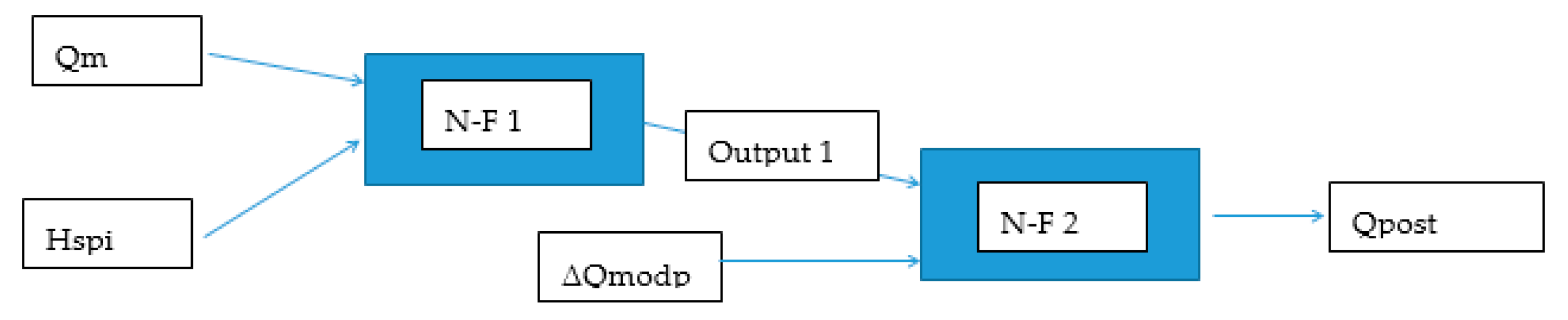
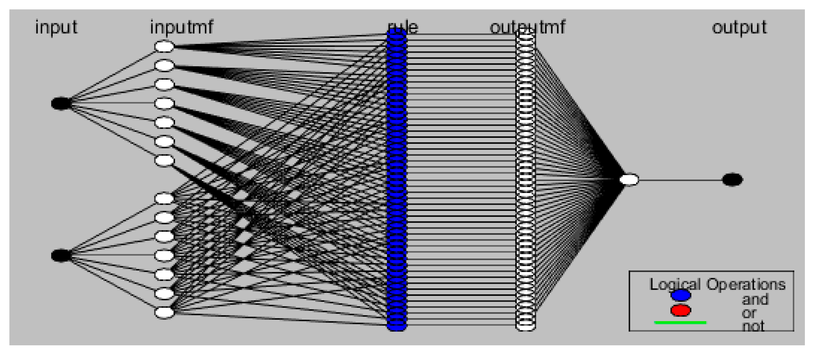
The best results in the validation stage were achieved using an architecture that used the current value of Qsim as input the gradient between the current and previous value ΔQmodp and the average of hourly precipitation total Hspi for the selected time period Γ [h]. The architecture described above will hereafter be referred to as the NFM 1 model. Figure 5 shows a diagram of the NFM 1 model and Figure 6 shows one of the local model (N-F).
The learning process itself took place in two phases. In the first phase, the architecture of the fuzzy model of Sugeno [18,19] type was constructed using the method of fuzzy C-mean clustering [20]. This step determines the value of the input and output, value and shape of membership function (mf) of the model and sets rule matrix. Then, training was performed on selected episodes using the backpropagation method and the use of the built-in function of the MATLAB anfis program [21]. The best results were obtained when the value of mf was set to 5 (Gaussian curve) for all local N-F models.
For the NFM model, an analysis of the influence of the length of the selected period of the Hspi parameter on the results was performed. The results of the analysis are shown in Table 3. The length of the chosen period for the calculation of Hspi is referred to as Γ in the following text.
It can be seen from Table 3 that the length values used to generate the Hspi parameter generally reach higher values for larger river basins. This statement corresponds to the length of the river basin’s reaction time to previous precipitation.
While testing the effect of length on the Γ parameter, the choice and number of training events were also tested. Based on the testing results, it was found that better results were achieved by selecting particular training episodes rather than using all the data. When choosing whether to use the training episode, two basic criteria were decisive. The first of these was the simulated peak flow, which should not differ by more than 25% from the value of the simulated peak flow of the adjusted episode. If the total number of training episodes was less than three, the 25% limit was gradually increased until at least one training episode was found. The second criterion was the maximum sum of the moving average of the total precipitation of a length three. If for the selected training episodes according to the first selection criterion, the maximum moving average of the three values differed by more than 60% from the adjusted episode and the total number of episodes was higher than five, episodes that did not meet the criterion were excluded. Figure 7 shows a comparison between an application of post-processing to a selected episode using all training episodes and using a selection of training episodes. Figure 8 shows training results for select episode June 2013 Bechyně (including artificial episode for training made by EEA).
4. Results
To better evaluate the results, an Ek criterion was introduced, which is defined as the average relative deviation between the actual value of the peak flow Qp,i and the predicted value Qs,i for the entire validation period, where the individual members are averaged in absolute values.
The Nash–Suctliffe criterion (NSE) was introduced to further evaluate the benefits of post-processing:
The root mean square error (RMSE) was chosen as the last criterion:
The individual results were further divided according to the N-year culmination into two groups (N ≤ 1 and N > 1). First, the overall results were evaluated and these were then evaluated separately for each group, because it was necessary to assess how the model performs under situations of different level of seriousness. The Ek criterion was introduced because the issuance of alerts is very often governed by the peak flow value.
Table 4 shows the criteria values for all profiles together for the whole validation period for the episodes when the above-mentioned post-processing and the values obtained for the data without post-processing (clean data) were used. The Ek and NSE values are averaged results for the whole validation period. The criterion E is the sum of the individual results of the criteria E for whole validation period.
The results in Table 4 show that the results obtained using post-processing brought improvements in the tested profiles in the range of 5–60% for the Ek criterion and 5–45% for the E criterion. An exception was the Sušice profile, where post-processing results of the Ek criterion deteriorated by 20% for all data. Furthermore, for the Bohumilice profile, there was a 0.5% deterioration in the criterion E. In case the deterioration or improvement rate is below 1%, the results obtained can be considered as the same (i.e., neither improved nor deteriorated). From the values in the Table 5, it is clear that the aggregated final values of the criteria when using post-processing are significantly lower than on clean data.
5. Discussion
From the previous text, it is clear that the introduction of post-processing brought a decrease in the values of all the criteria for most profiles. Only the Sušice profile deteriorated. A possible reason for this was that the results of the Aqualog model were very good for the profile, and the training base was very inconsistent in terms of underestimation (overestimation). The above-mentioned inconsistency is probably due to the area distribution of the precipitation that caused the flood wave. Part of the catchment area in the top part of Šumava is very poorly monitored by rain gauges, and therefore, in situations with orographic intensification of precipitation from the western direction, underestimation of precipitation is probably a major source of model errors. On the contrary, in the opposite direction of the air flow, more central parts of the basin are involved in the outflow, which are monitored very well. From this example, it can be seen that some difficulty with the success rate of the NFM method can be expected where different flood mechanisms lead to a different spectrum of sources of uncertainty in the hydrological flow modeling.
The main goal of the post-processing described above does not have to be the forecast of the flood episode directly, but only to provide information about the flood wave (peak flow and waveform) on the basis of which the hydrological forecast model settings can be corrected and the forecast recalculated.
A major limitation of the method described above is that for its use, the hydrological prediction model must run at all times without interventions and changes in the coefficients. Only then it is possible to identify certain relationships between the predictions of the hydrological model and the actual flows (determine the dependence of the model error). Two directories (settings, programs) of the hydrological forecasting model are needed for their use under normal operation.
When the peak flow for simulated flood is unknown, all data from the training matrix for the chosen month are used for the training model by algorithm, until the peak flow is found. This solution is not ideal, and therefore, it is better to wait until peak flow is known or (if it is possible) to prolong the length of forecast time when the peak flow is known. The model is built in a way, which enables post-processing of forecast (simulated flow) of a desired length.
Different numbers of time period values Γ were used to determine the Hspi parameter. The size of the number of previous values relatively corresponds to the size of the catchment area (Table 3) except for Profiles 4 and 9, which deviate significantly from the trend described above. The deviation from the trend can partly be explained by a more detailed examination of individual river basins. Profile 4 probably reduces the response time of the river basin to the previous precipitation due to large pond systems in its catchment, and therefore its size does not correspond to the trend of the Γ parameter. The entire catchment area of Profile 9 is located in the first stage of the protection zone of the Šumava National Park, so it can be assumed that there is a slower outflow of water from the catchment area compared to common catchments with agricultural areas and roads.
The EEA algorithm was introduced due to a small sample of extreme events. The EEA algorithm is used only when simulated peak flow (results of hydrological model) significantly overpowered values in historical data. The results (Figure 7) improved, but post-processing was not able to catch up with reality. This is caused by historical size of systematic error, which in the training set, did not exceed 20% of difference. The error in this episode (hydrological model) is due to the complex system of ponds, which is able to water transfer between river basins.
The algorithm for choosing events with similar peak flow and rainfall for the learning process was used, because size (tendency) of the systematic error is usually similar for similar events. When all events are used for learning process results were worse probably due to differ size or behavior of the systematic error. The hydrological model for certain values (events) can overestimate (underestimate) the results.
The results presented in Table 4 represent the average for the whole validation period and thus need to be treated accordingly. During the evaluation of the individual episodes, there was a significant improvement in some episodes compared to the table values. A disadvantage of the method described above remains the occurrence of atypical episodes that behave in the opposite way to the trend. One way to deal with this shortcoming would be to better categorize training data and find the causes of atypical behavior, but due to the relatively small database, this shortcoming could not be remedied. If the database was significantly larger, this shortcoming should be significantly mitigated. In addition, a larger data set should lead to better selection of events for training, which could lead to even better results than were achieved in this study.
The method is not suitable if there is a water reservoir (system of reservoirs) in the upper part of the river basin, which is able to significantly influence the water flow in the forecast profile. The reason being that the reservoir very often and unsystematically changes the shape and culmination of the flood wave due to its manipulation and can very easily disrupt the relationship (conditions) of the forecast error.
The results of all criteria are showed that method is more suitable for larger basins then smaller one. These results are clearly right and also misunderstanding, because method itself work with systematic error. The large basins have usually bigger systematic error due to more complex basin’s system. Small basins have often better schematization and therefore systematic error is smaller and find out its behavior is more difficult (a larger data set is needed). The method itself really does not care about parameters of basin (area, elevation, vegetation cover—only if training data are from similar vegetation period) as long as these parameters are rather stable, and therefore, do not cause a strong random error. If the systematic error is over noised by the random error, the method is more difficult to apply.
6. Conclusions
- The method was successfully applied on 12 profiles (base on chosen criteria).
- Improved forecast can lead to better estimation of risk.
- The method itself is transferable with certain limitation.
- The method has short calculation time and can be used for chosen length of forecast.
- The method is applied directly on hydrological model results (hydrological model do not have to be recalculated).
The method described in this article is intended for the purposes of post-processing the results computed by hydrological model. The goal is to further improve the hydrological prediction in situations of increased flows (flood events) caused by previous rainfall. For the purposes of testing the method, 12 prediction profiles were selected, for which various architectures and settings of post-processing models were tested during the validation period of 2010–2016. The initial results did not reach sufficient quality for some extreme values in the validation period, and therefore, an EEA algorithm was introduced. After the introduction of all corrections, there was a significant improvement (decrease) in the values of all criteria described above. For each prediction profile, the best results were obtained when only similar events were used during the learning process. Thus, there was no general assumption that all available data should be used for the learning process. When using post-processing (NFM model), better values were achieved for most of the tested events for all selected criteria compared to a classical calculation, i.e., without post-processing. Based on the achieved results, the contribution of NFM models as a post-processing tool can be stated.
The improvement of forecast values can help to lower the risk during the process of evaluating the danger in a particular basin. The improved forecast could lead to improved hit/miss/false statistic for particular forecasting profiles. (HIT—flood occurred, warning issued, MISS—flood occurred, warning not issued, FALSE—flood not occurred, warning issued). Post-processed values of events also showed lower values of the criterion E, therefore, the total volume of flood was also improved. This improvement should help to control the flood by water reservoir, which usually works with wave’s volume and peak. Profile Numbers 1, 2, 4 and 6 are used as inputs by the water reservoir to control floods.
The method itself is transferable and applicable to most river basins if there is a sufficient database for training the models. The method was devised as a tool to improve hydrological forecasts. For this purpose, both the upper and lower river basin were tested in this article. The river basin, which is located lower to downstream is already burdened with an error from the previous calculated river basin. The method achieved very good results even in the downstream river basins.
The main aim of this study was to test a trained neuro-fuzzy model as a tool for post-processing. The method described in the article does not require recalculation (re-calibration) of the whole model after or during flood event to function, unlike the most commonly used post-processing methods. Another benefit of this method is its short calculation time (few seconds) and the fact it can be used for any length of forecast.
Author Contributions
Writing—original draft preparation, T.K.; methodology, T.K.; simulations, T.K., T.V.; supervision, T.K. and P.J. All authors have read and agreed to the published version of the manuscript.
Funding
This research received no external funding.
Institutional Review Board Statement
Not applicable.
Informed Consent Statement
Not applicable.
Data Availability Statement
Data was obtained from Czech Hydrometeorological Institute and are available only with the permission of the Czech Hydrometeorological Institute.
Acknowledgments
The article was created with the support of a grant Ministry of the Interior-Program: Hydrometeorological Risks in the Czech Republic—Changes in Risks and Improvement of their Predictions VI20192021166.
Conflicts of Interest
The authors declare no conflict of interest.
References
- Krzysztofowicz, R. Bayesian Theory of Probabilistic Forecasting via Deterministic Hydrologic Model. Water Resour. Res. 1999, 35, 2739–2750. [Google Scholar] [CrossRef] [Green Version]
- Madadgar, S.; Moradkhani, H.; Garen, D. Towards improved post-processing of hydrologic forecast ensembles. Hydrol. Process. 2014, 28, 104–122. [Google Scholar] [CrossRef]
- Amezcua, J.; van Leeuwen, P.J. Time-correlated model error in the (ensemble) Kalman smoother. Q. J. R. Meteorol. Soc. 2018. [Google Scholar] [CrossRef] [PubMed] [Green Version]
- Li, W.; Duan, Q.; Miao, C.; Ye, A.; Gong, W.; Di, Z. A review on statistical postprocessing methods for hydrometeorological ensemble forecasting. Interdiscip. Rev. Water 2017, 4, e1246. [Google Scholar] [CrossRef]
- Xua, J.; Anctila, F.; Boucherb, M.-A. Hydrological post-processingof streamflow forecastsissued frommultimodel ensemble prediction systems. J. Hydrol. 2019, 578, 124002. [Google Scholar] [CrossRef]
- Ye, A.; Duan, Q.; Yuan, X.; Wood, E.-F.; Schaake, J. Hydrologic post-processing of MOPEX streamflow simulations. J. Hydrol. 2014, 508, 147–156. [Google Scholar] [CrossRef]
- Meinhold, R.J.; Singpurwalla, N.D. Understanding the Kalman Filter. Am. Stat. 1983, 37, 123–127. [Google Scholar] [CrossRef]
- Jang, J.S.R.; Sun, C.T. Neuro-Fuzzy Modelling and Control. Proc. IEEE 1995, 83, 378–406. [Google Scholar] [CrossRef]
- Bertoni, J.C.; Tucci, C.E.; Clarke, R.T. Rainfall-based real-time flood forecasting. J. Hydrol. 1992, 131, 313–339. [Google Scholar] [CrossRef]
- Nayak, P.; Sudheer, K.; Rangan, D.; Ramasastri, K. Short-term flood forecasting with a neurofuzzy model. Water Resour. Res. 2005, 41. [Google Scholar] [CrossRef] [Green Version]
- Kozel, T.; Stary, M. Adaptive stochastic management of the storage function for a large open reservoir using an artificial intelligence method. J. Hydrol. Hydromech. 2019, 67, 314–321. [Google Scholar] [CrossRef] [Green Version]
- Lin, Q.; Leandro, J.; Wu, W.; Bhola, P.; Disse, M. Prediction of Maximum Flood Inundation Extents with Resilient Backpropagation Neural Network: Case Study of Kulmbach. Front. Earth Sci. 2020, 8, 332. [Google Scholar] [CrossRef]
- Janal, P.; Stary, M. Fuzzy model used for the prediction of a state of emergency for a river basin in the case of a flash flood—Part 2. J. Hydrol. Hydromech. 2012, 60, 162–173. [Google Scholar] [CrossRef]
- Krejci, J.; Zezulak, J. The use of hydrological system AquaLog for flood warning service in the Czech Republic. In Proceedings of the May 2009 Conference: Regional Workshop on Hydrological Forecasting and Real Time Data Management, Dubrovnik, Croatia, 11–13 May 2009. [Google Scholar]
- Georgakakos, K.P. A generalized stochastic hydrometeorological model for flood and flash-flood forecasting: 1. Formulation. Water Resour. Res. 1986. [Google Scholar] [CrossRef]
- Anderson, E.A. A Point Energy and Mass Balance Model of a Snow Cover; NOAA Tech. Rep. NWS 19; National Oceanic and Atmospheric Administration: Silver Spring, MD, USA, 1976; 150p.
- Bras, R. Hydrology: An Introduction to Hydrologic Science; Addison-Wesley: Reading, MA, USA, 1990. [Google Scholar]
- Sugeno, M. Fuzzy Measures and Fuzzy Integrals. In Fuzzy Automata and Decision Processes; Gupta, M.M., Saridis, G.N., Ganies, B.R., Eds.; North-Holand: New York, NY, USA, 1977; pp. 89–102. [Google Scholar]
- Tagaki, H.; Sugeno, M. Fuzzy identification of systems and its applications to modelling and control. IEEE Trans. Syst. Man Cybern. 1985, 1, 116–132. [Google Scholar] [CrossRef]
- Bezdec, J.C. Pattern Recognition with Fuzzy Objective Function Algorithms; Plenum Press: New York, NY, USA, 1981. [Google Scholar]
- MATLAB and Fuzzy Logic Toolbox Release 2006a; The MathWorks, Inc.: Natick, MA, USA, 2006.
Figure 1.
Scheme of important process.

Figure 2.
Model scheme using sequential aggregation of inputs.

Figure 3.
Model scheme without using sequential aggregation of inputs.

Figure 4.
Locations of river profiles and their catchments.

Figure 5.
Schema of model NFM.

Figure 6.
Simplified schema of model local model NFM 1.

Figure 7.
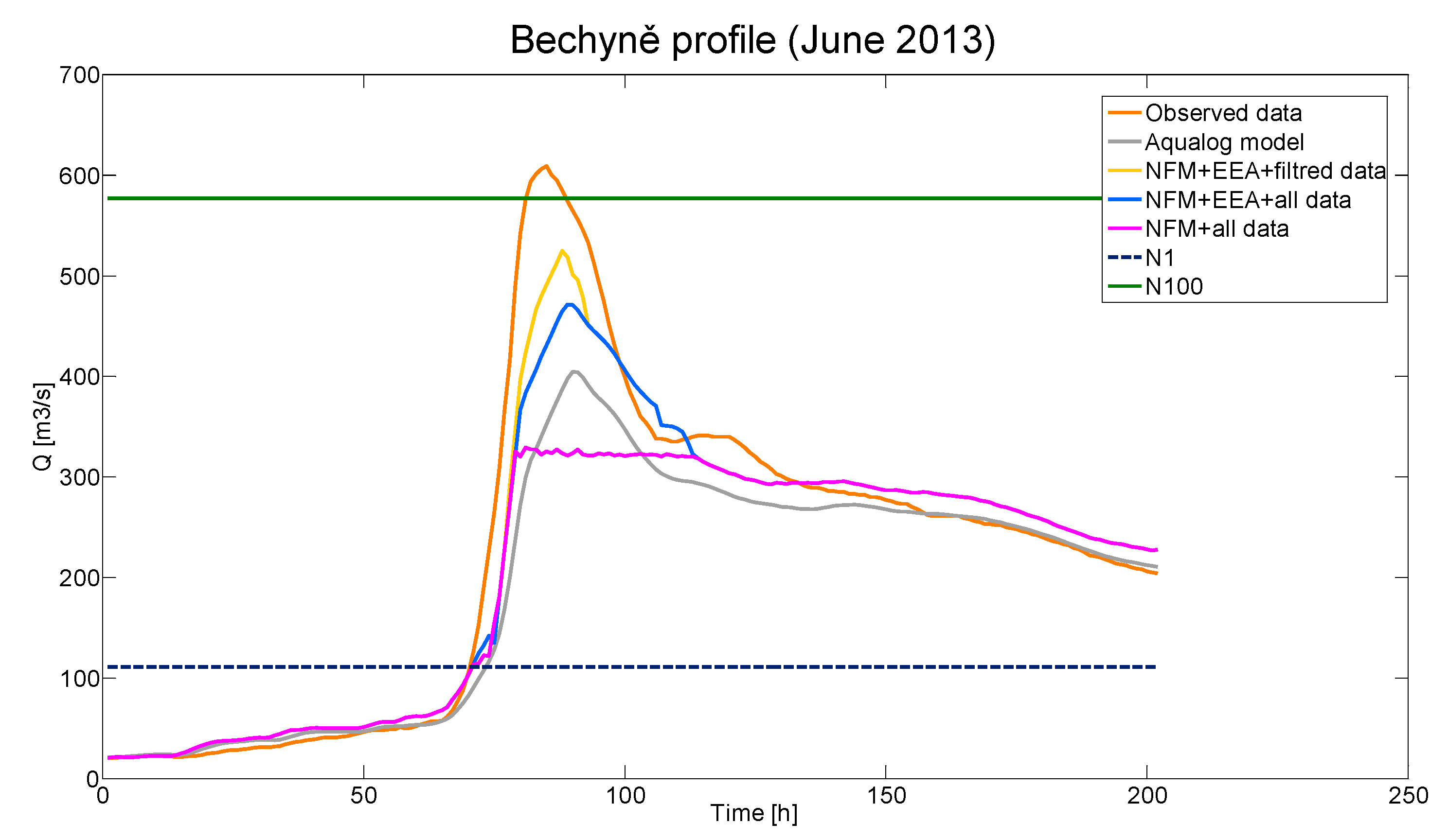
Results for the selected episode in the Bechyně profile. Figure 7 shows the course of the selected episode, where the dashed blue line shows the flow value N1 (period of return = 1) and the green value N100 (period of return = 100). The measured data are plotted in orange. The re-simulation of the episode using the Aqualog model is shown in gray. The results are shown in pink with the use of post-processing without the use of the EEA algorithm and the selection of episodes was not used during the training. The results of post-processing using the EEA algorithm during training and without selection of individual episodes are displayed in blue. The yellow color shows the results using post-processing using the EEA algorithm during training and using the selection of episodes.
Figure 7.
Results for the selected episode in the Bechyně profile. Figure 7 shows the course of the selected episode, where the dashed blue line shows the flow value N1 (period of return = 1) and the green value N100 (period of return = 100). The measured data are plotted in orange. The re-simulation of the episode using the Aqualog model is shown in gray. The results are shown in pink with the use of post-processing without the use of the EEA algorithm and the selection of episodes was not used during the training. The results of post-processing using the EEA algorithm during training and without selection of individual episodes are displayed in blue. The yellow color shows the results using post-processing using the EEA algorithm during training and using the selection of episodes.

Figure 8.
Calibration results for the selected episode in the Bechyně profile. Figure 8 plots the training data (blue) and the result of the trained post-processing model (red). An artificial training episode provided by the EEA algorithm is also shown (black circles).
Figure 8.
Calibration results for the selected episode in the Bechyně profile. Figure 8 plots the training data (blue) and the result of the trained post-processing model (red). An artificial training episode provided by the EEA algorithm is also shown (black circles).


Table 1.
Parameters used for model construction.
| Value | Marking | Unit |
|---|---|---|
| Instantaneous flow value | Qsim | m3/s |
| Total precipitation amount (1 h) | Hs | Mm |
| Previous flow value | Qpm | m3/s |
| Next flow value | Qfm | m3/s |
| Topsoil saturation indicator | UTWZ | Mm |
| Average of the hourly sum of precipitation totals over a period of time | Hspi | Mm |
| Corrected flow (post-procesing flow) | Qpost | m3/s |
| Difference between current and previous flow value | ΔQmodp | m3/s |
| Difference between current and next flow value | ΔQmodf | m3/s |
| Average of the flow values over time | Qpmodi | m3/s |
Table 2.
Profile specification.
| Num. | Profile | River | Catchment Area [km2 ] | Qa [m3/s] | 1. FLD [m3/s] | 2. FLD [m3/s] | 3. FLD [m3/s] | N1 [m3/s] | N100 [m3/s] | FIP [%] |
|---|---|---|---|---|---|---|---|---|---|---|
| 1 | České Budejovice | Vltava | 2850 | 106 | 244 | 361 | 489 | 172 | 908 | 35 |
| 2 | Lenora | Tepla Vltava | 177 | 3.06 | 29 | 53.5 | 70.8 | 26 | 113 | 78 |
| 3 | Ličov | Cerna | 127 | 1.29 | 12.7 | 21.4 | 29.7 | 21 | 188 | 53 |
| 4 | Bechyně | Luznice | 4057 | 22.2 | 87.9 | 140 | 187 | 111 | 577 | 33 |
| 5 | Rodvínov | Nezarka | 297 | 2.2 | 18.7 | 26.9 | 43.7 | 20 | 91 | 10 |
| 6 | Písek | Otava | 2914 | 23.4 | 135 | 214 | 297 | 146 | 837 | 27 |
| 7 | Katovice | Otava | 1134 | 13.8 | 118 | 169 | 255 | 133 | 510 | 42 |
| 8 | Sušice | Otava | 533 | 10.5 | 64.2 | 94.3 | 127 | 101 | 369 | 77 |
| 9 | Modrava | Vydra | 90 | 3.01 | 30.5 | 41.2 | 54.6 | 29 | 120 | 96 |
| 10 | Stodůlky | Kremelna | 135 | 3.24 | 24 | 37 | 52.4 | 40 | 153 | 89 |
| 11 | Bohumilice | Spulka | 105 | 0.97 | 24 | 35.1 | 47.7 | 11 | 84 | 48 |
| 12 | Podedvory | Blanice | 204 | 2.04 | 15.3 | 28.2 | 38.6 | 25 | 165 | 60 |
Table 3.
Values of Γ, for which the lowest values of the selected criteria were reached.
| Num. Basin | 1 | 2 | 3 | 4 | 5 | 6 | 7 | 8 | 9 | 10 | 11 | 12 |
|---|---|---|---|---|---|---|---|---|---|---|---|---|
| Γ [h] | 6 | 2 | 2 | 4 | 3 | 6 | 6 | 5 | 3 | 2 | 2 | 3 |
| Area [km2] | 2848 | 177 | 127 | 4057 | 297 | 2914 | 1134 | 534 | 90 | 135 | 105 | 203 |
Table 4.
Criteria results for the individual profiles.
| Name: České Budějovice (Area = 2850 km2, N1 = 172 m3/s) | ||||||
|---|---|---|---|---|---|---|
| Method | Post-procesing | Clean data | ||||
| Data set | All | N > 1 | N < 1 | All | N > 1 | N < 1 |
| Ek | 0.33 | - | 0.33 | 0.63 | - | 0.63 |
| E | 665 | - | 665 | 1539 | - | 1539 |
| RMSE | 2.44 | - | 2.44 | 3.44 | - | 3.44 |
| NSE | 0.77 | - | 0.77 | 0.70 | 0.70 | |
| Num. events | 24 | 0 | 24 | 24 | 0 | 24 |
| Name: Lenora (Area 177 = km2, N1 = 26 m3/s) | ||||||
| Method | Post-procesing | Clean data | ||||
| Data set | All | N > 1 | N < 1 | All | N > 1 | N < 1 |
| Ek | 0.23 | 0.24 | 0.23 | 0.38 | 0.22 | 0.40 |
| E | 559 | 3092 | 228 | 1074 | 5081 | 551 |
| RMSE | 2.16 | 4.10 | 1.79 | 3.03 | 5.02 | 2.93 |
| NSE | 0.81 | 0.86 | 0.80 | 0.77 | 0.81 | 0.77 |
| Num. events | 26 | 3 | 23 | 26 | 3 | 23 |
| Name: Ličov (Area = 127 km2, N1 = 21 m3/s) | ||||||
| Method | Post-procesing | Clean data | ||||
| Data set | All | N > 1 | N < 1 | All | N > 1 | N < 1 |
| Ek | 0.35 | 0.33 | 0.36 | 0.37 | 0.38 | 0.37 |
| E | 1138 | 3972 | 429 | 1249 | 4788 | 364 |
| RMSE | 2.31 | 2.41 | 2.67 | 2.54 | 2.73 | 2.45 |
| NSE | 0.65 | 0.71 | 0.63 | 0.62 | 0.69 | 0.60 |
| Num. events | 20 | 4 | 16 | 20 | 4 | 16 |
| Name: Bechyně (Area = 4057 km2, N1 = 111 m3/s) | ||||||
| Method | Post-procesing | Clean data | ||||
| Data set | All | N > 1 | N < 1 | All | N > 1 | N < 1 |
| Ek | 0.09 | 0.07 | 0.02 | 0.14 | 0.14 | 0.03 |
| E | 596,330 | 715,530 | 331 | 952,960 | 1,143,461 | 453 |
| RMSE | 15.23 | 24.55 | 1.55 | 17.23 | 26.93 | 1.79 |
| NSE | 0.94 | 0.93 | 0.99 | 0.91 | 0.89 | 0.98 |
| Num. events | 6 | 5 | 1 | 6 | 5 | 1 |
| Name: Rodvínov (Area = 297 km2, N1 = 20 m3/s) | ||||||
| Method | Post-procesing | Clean data | ||||
| Data set | All | N > 1 | N < 1 | All | N > 1 | N < 1 |
| Ek | 0.31 | 0.32 | 0.26 | 0.39 | 0.32 | 0.41 |
| E | 2711 | 5476 | 2020 | 3231.02 | 6476 | 2420 |
| RMSE | 5.21 | 5.65 | 4.72 | 6.07 | 11.53 | 5.71 |
| NSE | 0.6 | 0.66 | 0.56 | 0.58 | 0.66 | 0.52 |
| Num. events | 5 | 1 | 4 | 5 | 1 | 4 |
| Name: Písek (Area = 2914 km2, N1 = 146 m3/s) | ||||||
| Method | Post-procesing | Clean data | ||||
| Data set | All | N > 1 | N < 1 | All | N > 1 | N < 1 |
| Ek | 0.10 | 0.07 | 0.17 | 0.12 | 0.07 | 0.22 |
| E | 18,062 | 22,748 | 16,890 | 21,276 | 27,573 | 19,402 |
| RMSE | 12.62 | 11.75 | 14.13 | 15.11 | 14.16 | 16.78 |
| NSE | 0.81 | 0.94 | 0.77 | 0.77 | 0.87 | 0.75 |
| Num. events | 20 | 4 | 16 | 20 | 4 | 16 |
| Name: Katovice (Area = 1134 km2, N1 = 137 m3/s) | ||||||
| Method | Post-procesing | Clean data | ||||
| Data set | All | N > 1 | N < 1 | All | N > 1 | N < 1 |
| Ek | 0.09 | 0.12 | 0.08 | 0.15 | 0.18 | 0.15 |
| E | 3806 | 12,554 | 1965 | 6846 | 14,946 | 5141 |
| RMSE | 6.36 | 10.54 | 5.21 | 9.17 | 11.94 | 8.17 |
| NSE | 0.83 | 0.94 | 0.81 | 0.81 | 0.91 | 0.79 |
| Num. events | 23 | 4 | 19 | 23 | 4 | 19 |
| Name: Sušice (Area = 533 km2, N1 = 101 m3/s) | ||||||
| Method | Post-procesing | Clean data | ||||
| Data set | All | N > 1 | N < 1 | All | N > 1 | N < 1 |
| Ek | 0.11 | 0.12 | 0.09 | 0.09 | 0.14 | 0.08 |
| E | 3806 | 9726 | 1500 | 3843 | 7294 | 3046 |
| RMSE | 7.76 | 14.39 | 4.28 | 7.78 | 11.58 | 6.81 |
| NSE | 0.80 | 0.86 | 0.78 | 0.61 | 0.83 | 0.56 |
| Num. events | 16 | 3 | 13 | 16 | 3 | 13 |
| Name: Modrava (Area = 90 km2, N1 = 29 m3/s) | ||||||
| Method | Post-procesing | Clean data | ||||
| Data set | All | N > 1 | N < 1 | All | N > 1 | N < 1 |
| Ek | 0.28 | 0.27 | 0.28 | 0.43 | 0.30 | 0.45 |
| E | 1096 | 3839 | 613 | 1311 | 3621 | 903 |
| RMSE | 3.73 | 8.11 | 2.95 | 4.50 | 7.99 | 3.88 |
| NSE | 0.83 | 0.71 | 0.86 | 0.64 | 0.7 | 0.62 |
| Num. events | 20 | 3 | 17 | 20 | 3 | 17 |
| Name: Stodůlky (Area = 135 km2, N1 = 40 m3/s) | ||||||
| Method | Post-procesing | Clean data | ||||
| Data set | All | N > 1 | N < 1 | All | N > 1 | N < 1 |
| Ek | 0.31 | 0.31 | 0.31 | 0.36 | 0.34 | 0.36 |
| E | 732 | 2889 | 463 | 1093 | 4035 | 726 |
| RMSE | 2.86 | 6.31 | 2.43 | 3.73 | 7.25 | 3.29 |
| NSE | 0.68 | 0.74 | 0.67 | 0.53 | 0.63 | 0.51 |
| Num. events | 27 | 3 | 24 | 27 | 3 | 24 |
| Name: Bohumilice (Area = 105 km2, N1 = 11 m3/s) | ||||||
| Method | Post-procesing | Clean data | ||||
| Data set | All | N > 1 | N < 1 | All | N > 1 | N < 1 |
| Ek | 0.57 | 0.45 | 0.59 | 0.96 | 0.46 | 1.05 |
| E | 177 | 678 | 89 | 176 | 674 | 88 |
| RMSE | 1.54 | 3.44 | 1.20 | 1.52 | 3.42 | 1.19 |
| NSE | 0.75 | 0.63 | 0.78 | 0.61 | 0.61 | 0.61 |
| Num. events | 20 | 3 | 17 | 20 | 3 | 17 |
| Name: Podedvory (Area = 204 km2, N1 = 25 m3/s) | ||||||
| Method | Post-procesing | Clean data | ||||
| Data set | All | N > 1 | N < 1 | All | N > 1 | N < 1 |
| Ek | 0.17 | 0.14 | 0.18 | 0.18 | 0.21 | 0.17 |
| E | 1681 | 2902 | 1070 | 2598 | 6141 | 827 |
| RMSE | 3.46 | 3.69 | 3.78 | 3.75 | 4.50 | 3.27 |
| NSE | 0.75 | 0.76 | 0.74 | 0.62 | 0.63 | 0.61 |
| Num. events | 15 | 5 | 10 | 15 | 5 | 10 |
Table 5.
Criteria results over all values.
| Criteria | Post-Procesing | Clean Data | ||||
|---|---|---|---|---|---|---|
| All | N > 1 | N < 1 | All | N > 1 | N < 1 | |
| Ek | 0.25 | 0.22 | 0.21 | 0.34 | 0.26 | 0.31 |
| E | 52,500 | 71,218 | 2133 | 83,099 | 111,281 | 2851 |
Publisher’s Note: MDPI stays neutral with regard to jurisdictional claims in published maps and institutional affiliations. |
© 2021 by the authors. Licensee MDPI, Basel, Switzerland. This article is an open access article distributed under the terms and conditions of the Creative Commons Attribution (CC BY) license (https://creativecommons.org/licenses/by/4.0/).
Share and Cite
MDPI and ACS Style
Kozel, T.; Vlasak, T.; Janal, P. Possibilities of Using Neuro-Fuzzy Models for Post-Processing of Hydrological Forecasts. Water 2021, 13, 1894. https://doi.org/10.3390/w13141894
AMA Style
Kozel T, Vlasak T, Janal P. Possibilities of Using Neuro-Fuzzy Models for Post-Processing of Hydrological Forecasts. Water. 2021; 13(14):1894. https://doi.org/10.3390/w13141894
Chicago/Turabian StyleKozel, Tomas, Tomas Vlasak, and Petr Janal. 2021. "Possibilities of Using Neuro-Fuzzy Models for Post-Processing of Hydrological Forecasts" Water 13, no. 14: 1894. https://doi.org/10.3390/w13141894
Note that from the first issue of 2016, this journal uses article numbers instead of page numbers. See further details here.