
Leakage Management and Pipe System Efficiency. Its Influence in the Improvement of the Efficiency Indexes

 , ,
, ,  and
and 
Abstract
:1. Introduction
2. Leakages Evaluation and KPIs
2.1. Torricelli Teorem
2.2. Minimum Night Flow (MNF) Analysis
2.3. FAVAD Concept
2.4. FAVAD and the N1 Power Law
2.5. Background Leakage and Emitter Coefficient (BABE)
2.6. Summary of Leak Calculation Methodologies
2.7. Leakages Modelling and Calibration
2.8. Leakages Key Performance Indicators (LKPIs)
- (1)
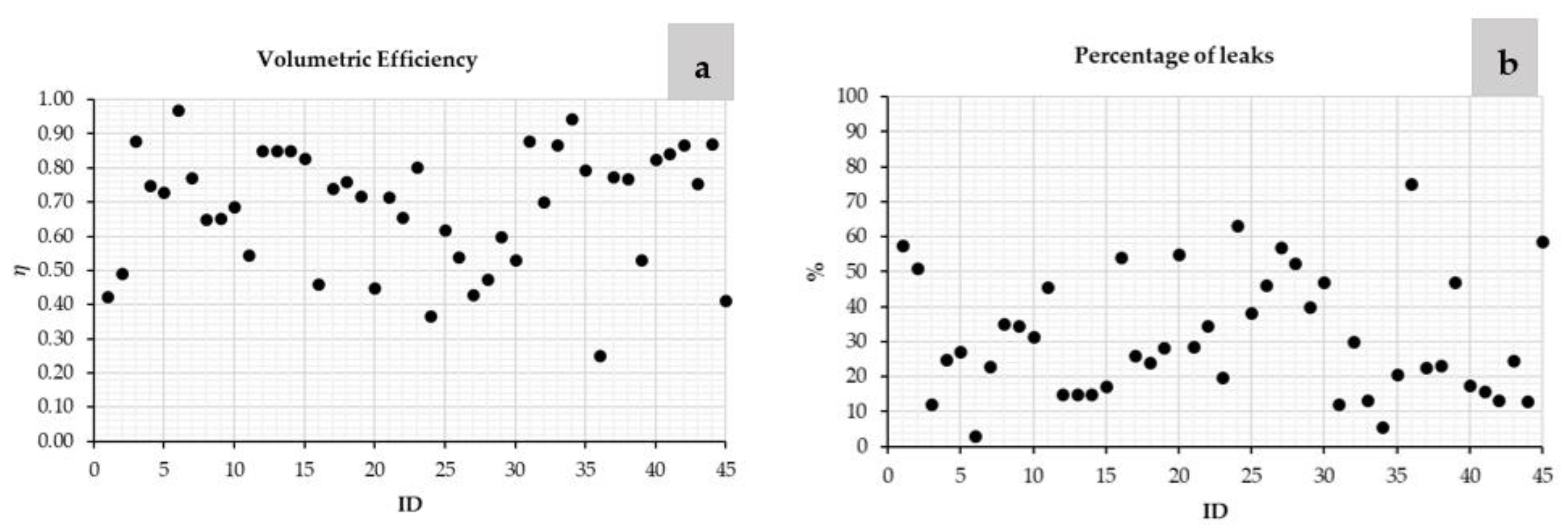
- Volumetric efficiency (); One of the most important ratios among the system’s efficiency indicators is volumetric performance. It is defined as the relationship between the registered volume and the total volume contributed in the same reference period [102]:
- (2)
- Performance Indicators for Water Supply Services; International water association (IWA) provides performance indicators of water supply systems to compare the management of water losses, these are (i) Water losses and real losses as a % of system input volume; (ii) Water losses per house connection and km of mains per day , and (iii) Infrastructure Leakage Index (ILI) [103].
- (3)
- Infrastructure Leakage Index (ILI); The ILI is a measure of how well a distribution network is managed (maintained, repaired, rehabilitated, etc.) for the control of real losses, at the current operating pressure. It is the ratio of the Current Annual volume of Real Losses (CARL) to Unavoidable Annual Real Losses (UARL) [104].
- (4)
- Unavoidable Annual Real Losses (UARL); UARL is a useful concept as it can be used to predict the lowest technically annual real losses for any combination of mains length , number of connections , customer meter location and average operating pressure assuming that the system is in good condition with high standards for the management of real losses [105].
- (5)
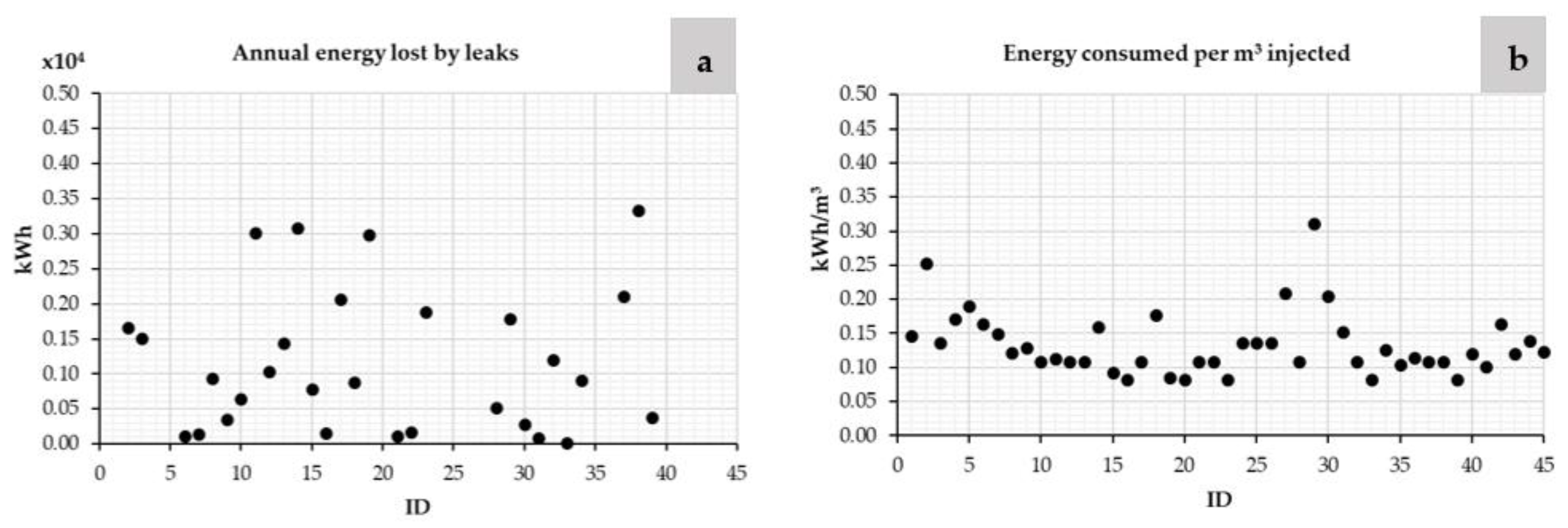
- Absolute annual consumed energy (IAAE); this index is sum of the total active consumed energy in the network subtracted by the sum of the total energy recovered in the network, the units are [106].
- (6)
- Absolute consumed energy per unit volume (IAEFW); Ratio between IAAE and the total volume of water introduced in the network, the units are [107].
3. Results
3.1. Case Studies
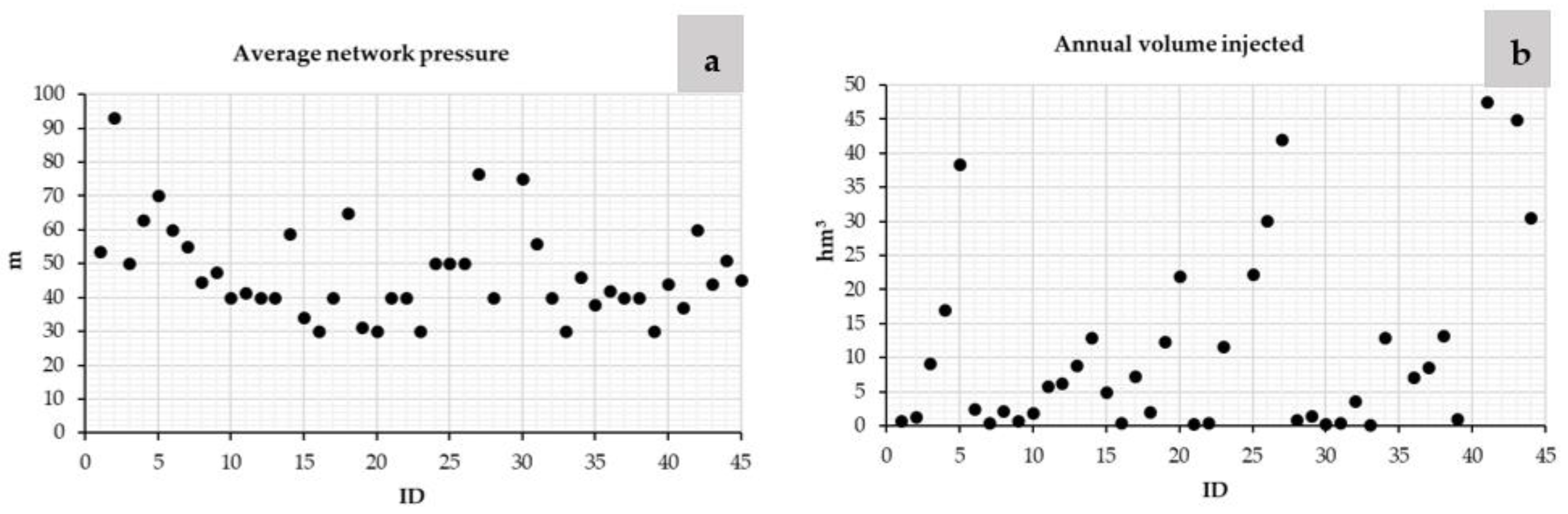
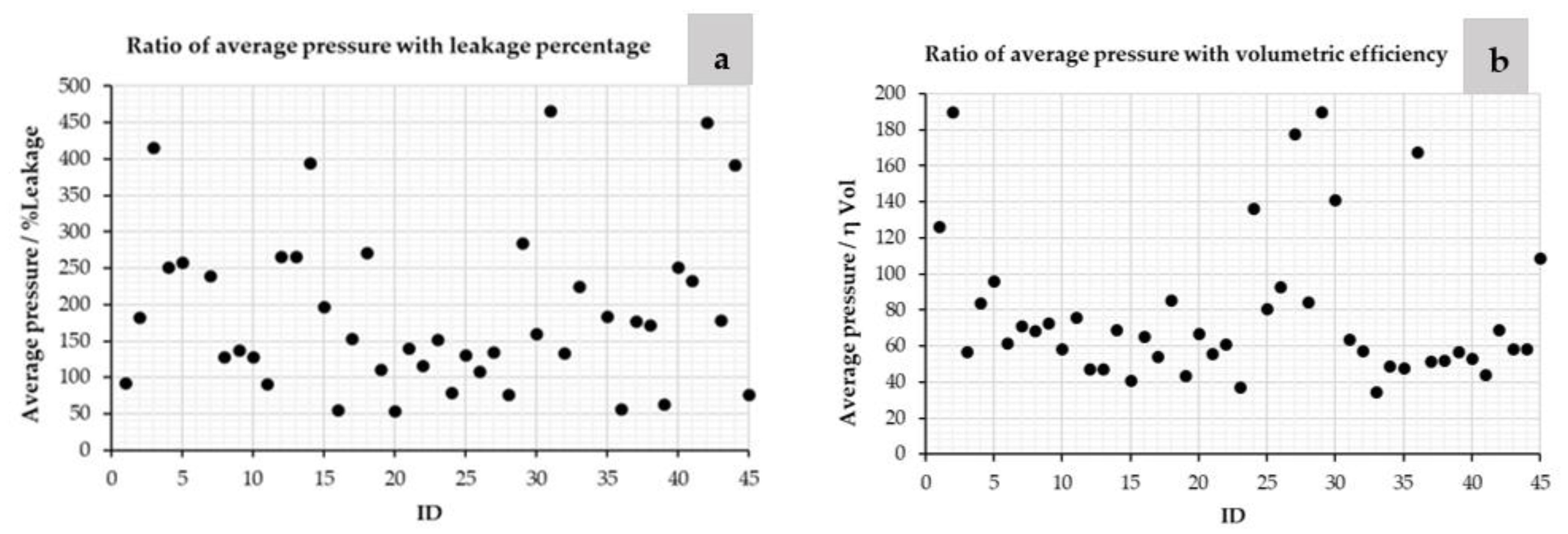
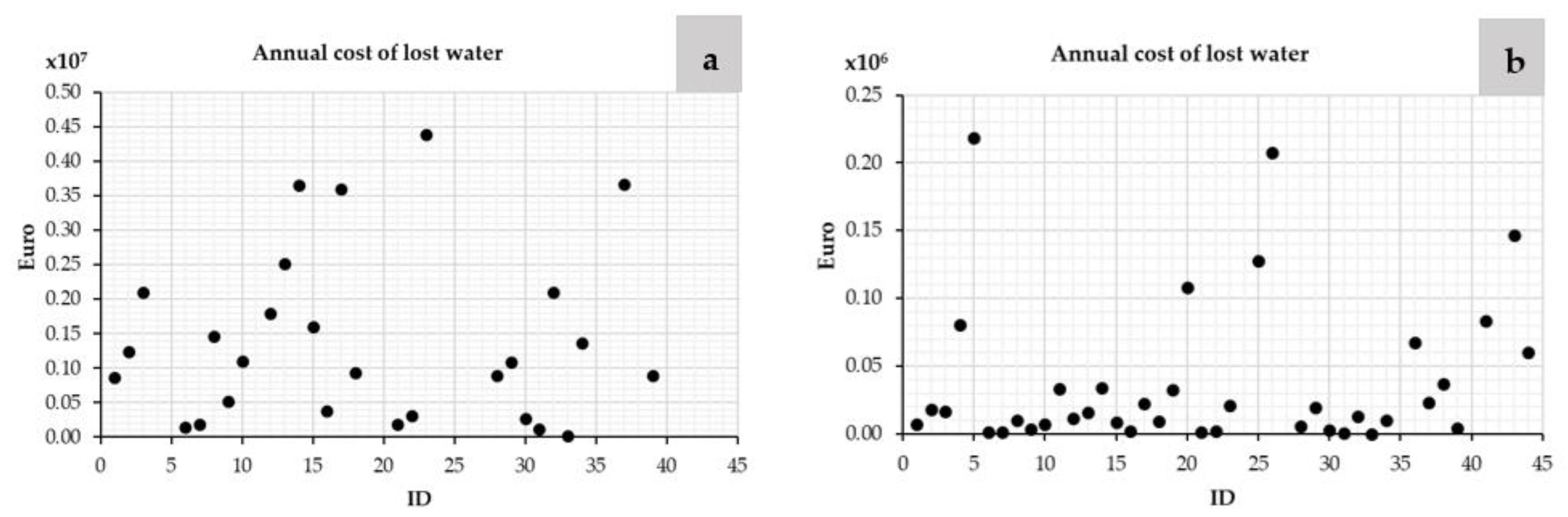
3.2. Influence of the Leakages in the KPI of the Water Systems
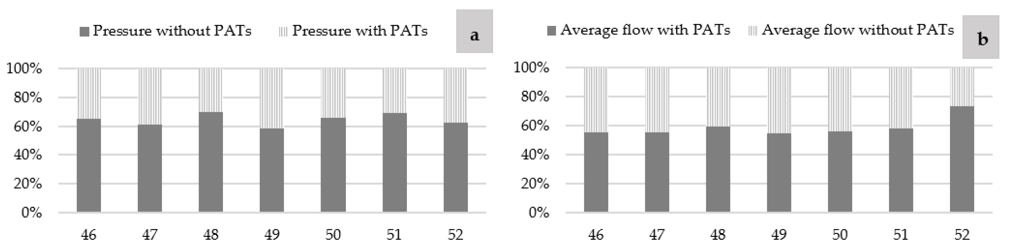
3.3. Pump Working as Turbine Using Leakages Models
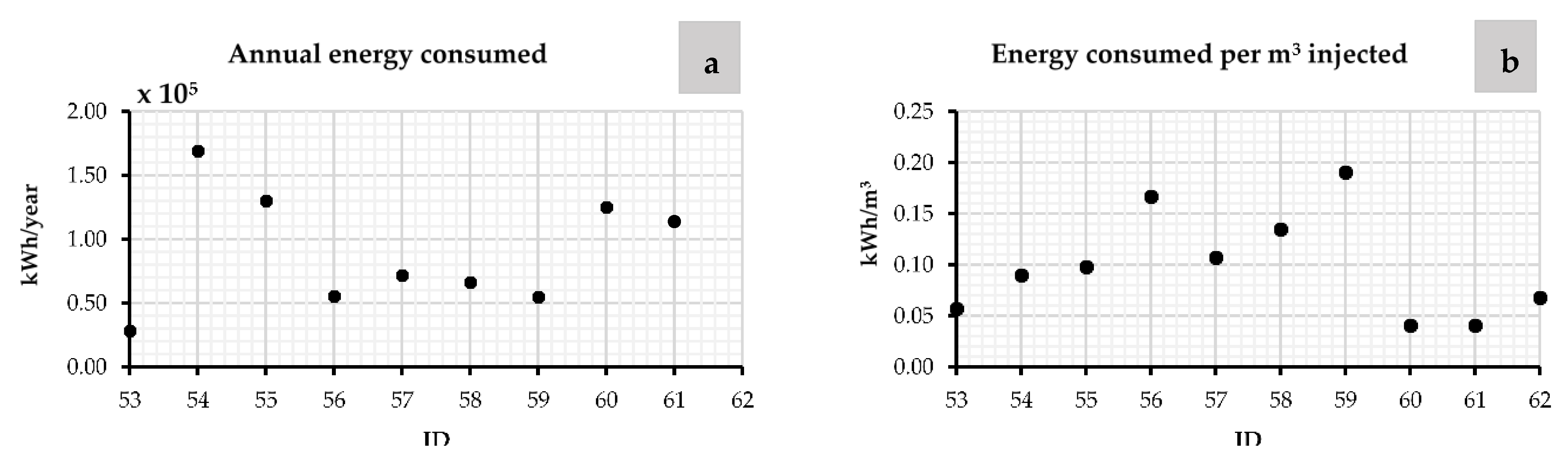
3.4. Energy Index Calculation Case Study
4. Conclusions
Author Contributions
Funding
Institutional Review Board Statement
Informed Consent Statement
Data Availability Statement
Conflicts of Interest
References
- Rojek, I.; Studzinski, J. Detection and localization of water leaks in water nets supported by an ICT system with artificial intelligence methods as away forward for smart cities. Sustainability 2019, 11, 518. [Google Scholar] [CrossRef] [Green Version]
- Farley, M. Leakage Management and Control; WHO: Geneva, Switzerland, 2001; pp. 1–98. [Google Scholar]
- Öztürk, I.; Uyak, V.; Çakmakci, M.; Akça, L. Dimension of water loss through distribution system and reduction methods in Turkey. Int. Congr. River Basin Manag. 2007, 1, 22–24. [Google Scholar]
- Maskit, M.; Ostfeld, A. Leakage Calibration of Water Distribution Networks. Procedia Eng. 2014, 89, 664–671. [Google Scholar] [CrossRef] [Green Version]
- Germanopoulos, G. A technical note on the inclusion of pressure dependent demand and leakage terms in water supply network models. Civ. Eng. Syst. 1985, 2, 171–179. [Google Scholar] [CrossRef]
- Adedeji, K.B.; Hamam, Y.; Abe, B.T.; Abu-Mahfouz, A.M. Towards Achieving a Reliable Leakage Detection and Localization Algorithm for Application in Water Piping Networks: An Overview. IEEE Access 2017, 5, 20272–20285. [Google Scholar] [CrossRef]
- Meniconi, S.; Capponi, C.; Frisinghelli, M.; Brunone, B. Leak Detection in a Real Transmission Main through Transient Tests: Deeds and Misdeeds. Water Resour. Res. 2021, 57. [Google Scholar] [CrossRef]
- Duan, H.-F.; Pan, B.; Wang, M.; Chen, L.; Zheng, F.; Zhang, Y. State-of-the-art review on the transient flow modeling and utilization for urban water supply system (UWSS) management. J. Water Supply Res. Technol. 2020, 69, 858–893. [Google Scholar] [CrossRef]
- Ayati, A.H.; Haghighi, A.; Lee, P.J. Statistical Review of Major Standpoints in Hydraulic Transient-Based Leak Detection. J. Hydraul. Struct. 2019, 5. [Google Scholar] [CrossRef]
- Modeling, N.; Leak, O.F.; On, E.; Behavior, T. Transient test-based technique for leak detection in outfall pipes. J. Water Resour. Plan. Manag. 1999, 125, 302–306. [Google Scholar]
- Capponi, C.; Ferrante, M.; Zecchin, A.C.; Gong, J. Leak Detection in a Branched System by Inverse Transient Analysis with the Admittance Matrix Method. Water Resour. Manag. 2017, 31, 4075–4089. [Google Scholar] [CrossRef] [Green Version]
- Adachi, S.; Takahashi, S.; Zhang, X.; Umeki, M.; Tadokoro, H. Estimation of Area Leakage in Water Distribution Networks: A Real Case Study. Procedia Eng. 2015, 119, 4–12. [Google Scholar] [CrossRef] [Green Version]
- Garcia, F.; Avilés-Añazco, A.; Ordoñez-Jara, J.; Guanuchi-Quezada, C. Pressure management for leakage reduction using pressure reducing valves. Case study in an Andean City. Alex. Eng. J. 2019, 58, 1313–1326. [Google Scholar] [CrossRef]
- Rajani, B.; Kleiner, Y. Comprehensive review of structural deterioration of water mains: Physically based models. Urban. Water 2001, 3, 151–164. [Google Scholar] [CrossRef] [Green Version]
- Almandoz, J.; Cabrera, E.; Arregui, F.; Cobacho, R. Leakage Assessment through Water Distribution Network Simulation. J. Water Resour. Plan. Manag. 2005, 131, 458–466. [Google Scholar] [CrossRef]
- Samir, N.; Kansoh, R.; Elbarki, W.; Fleifle, A. Pressure control for minimizing leakage in water distribution systems. Alex. Eng. J. 2017, 56, 601–612. [Google Scholar] [CrossRef]
- Ulanicki, B.; Skworcow, P.; Ulanicki, B.; Skworcow, P. Why PRVs Tends to Oscillate at Low Flows. Procedia Eng. 2014, 89, 378–385. [Google Scholar] [CrossRef] [Green Version]
- Abdelmeguid, H.; Skworcow, P.; Ulanicki, B. Mathematical modelling of a hydraulic controller for PRV flow modulation. J. Hydroinformatics 2011, 13, 374–389. [Google Scholar] [CrossRef] [Green Version]
- Ali, M.E. Knowledge-Based Optimization Model for Control Valve Locations in Water Distribution Networks. J. Water Resour. Plan. Manag. 2015, 141, 04014048. [Google Scholar] [CrossRef]
- Creaco, E.; Pezzinga, G. Multiobjective Optimization of Pipe Replacements and Control Valve Installations for Leakage Attenuation in Water Distribution Networks. J. Water Resour. Plan. Manag. 2015, 141, 04014059. [Google Scholar] [CrossRef]
- Meniconi, S.; Brunone, B.; Mazzetti, E.; Laucelli, D.B.; Borta, G. Hydraulic characterization and transient response of pressure reducing valves: Laboratory experiments. J. Hydroinformatics 2017, 19, 798–810. [Google Scholar] [CrossRef]
- Meniconi, S.; Brunone, B.; Ferrante, M.; Mazzetti, E.; Laucelli, D.B.; Borta, G. Transient Effects of Self-adjustment of Pressure Reducing Valves. Procedia Eng. 2015, 119, 1030–1038. [Google Scholar] [CrossRef] [Green Version]
- Ramos, H.M.; Borga, A. Pumps as turbines: An unconventional solution to energy production. Urban. Water 1999, 1, 261–263. [Google Scholar] [CrossRef]
- Novara, D.; Carravetta, A.; McNabola, A.; Ramos, H.M. Cost Model for Pumps as Turbines in Run-of-River and In-Pipe Microhydropower Applications. J. Water Resour. Plan. Manag. 2019, 145, 04019012. [Google Scholar] [CrossRef]
- De Marchis, M.; Fontanazza, C.; Freni, G.; Messineo, A.; Milici, B.; Napoli, E.; Notaro, V.; Puleo, V.; Scopa, A. Energy Recovery in Water Distribution Networks. Implementation of Pumps as Turbine in a Dynamic Numerical Model. Procedia Eng. 2014, 70, 439–448. [Google Scholar] [CrossRef] [Green Version]
- Jain, S.V.; Patel, R.N. Investigations on pump running in turbine mode: A review of the state-of-the-art. Renew. Sustain. Energy Rev. 2014, 30, 841–868. [Google Scholar] [CrossRef]
- Ebrahimi, S.; Riasi, A.; Kandi, A. Selection optimization of variable speed pump as turbine (PAT) for energy recovery and pressure management. Energy Convers. Manag. 2021, 227, 113586. [Google Scholar] [CrossRef]
- Al-Washali, T.; Sharma, S.; Al-Nozaily, F.; Haidera, M.; Kennedy, M. Modelling the Leakage Rate and Reduction Using Minimum Night Flow Analysis in an Intermittent Supply System. Water 2018, 11, 48. [Google Scholar] [CrossRef] [Green Version]
- Adedeji, K.B.; Hamam, Y.; Abe, B.T.; Abu-Mahfouz, A.M. Leakage Detection and Estimation Algorithm for Loss Reduction in Water Piping Networks. Water 2017, 9, 773. [Google Scholar] [CrossRef] [Green Version]
- Laucelli, D.B.; Meniconi, S. Water distribution network analysis accounting for different background leakage models. Procedia Eng. 2015, 119, 680–689. [Google Scholar] [CrossRef] [Green Version]
- Darsana, P.; Varija, K. Leakage detection studies for water supply systems—A review. Water Resour. Manag. 2018, 78, 141–150. [Google Scholar]
- Guo, S.; Zhang, T.-Q.; Shao, W.-Y.; Zhu, D.Z.; Duan, Y.-Y. Two-dimensional pipe leakage through a line crack in water distribution systems. J. Zhejiang Univ. A 2013, 14, 371–376. [Google Scholar] [CrossRef] [Green Version]
- Morales, E.; José, J.; Cabrera, E.; Cobacho, R. Método de los Caudales Minimos Nocturnos: Revisión De Sus Bases Científicas, Evaluación de Errores Potenciales y Propuestas Para su Mejora. Master’s Thesis, Universitat Politècnica de València, Valencia, España, 2011. Volume 146. pp. 17–20. [Google Scholar]
- Lambert, A.; Fantozzi, M.; Shepherd, M. Pressure: Leak flow rates using FAVAD: An improved fast-track practitioner’s approach. In Proceedings of the 15th International Conference on Computing and Control for the Water Industry, CCWI 2017, Sheffield, UK, 5–7 September 2017. [Google Scholar]
- Sellés, E.G. Caracterización y Mejora de la Eficiencia Energética del Transporte de Agua a Presión; Univ. Politécnica: Valencia, España, 2016; p. 384. [Google Scholar]
- Morales, E.; José, J. Ambiente Título del Trabajo Fin de Máster: Método de los Caudales Minimos Nocturnos: Intensificación: Autor: Máster en Ingeniería Hidráulica y Medio. Master’s Thesis, Universitat Politècnica de Valencia, Valencia, España, 2011. [Google Scholar]
- Lambert, A. What Do We Know About Pressure: Leakage Relationships in Distribution Systems? In Proceedings of the IWA Specialised Conference: System Approach to Leakage Control and Water Distribution Systems Management, Brno, Czech Republic, 16–18 May 2000; pp. 1–8. [Google Scholar]
- Rossman, L.A. The EPANET programmer’s toolkit for analysis of water distribution systems. In Proceedings of the WRPMD’99: Preparing for the 21st Century, Tempe, Arizona, 6–9 June 1999; pp. 1–10. [Google Scholar]
- Araujo, L.S.; Ramos, H.; Coelho, S.T. Pressure Control for Leakage Minimisation in Water Distribution Systems Management. Water Resour. Manag. 2006, 20, 133–149. [Google Scholar] [CrossRef]
- García, I.F.; Novara, D.; Mc Nabola, A. A Model for Selecting the Most Cost-Effective Pressure Control Device for More Sustainable Water Supply Networks. Water 2019, 11, 1297. [Google Scholar] [CrossRef] [Green Version]
- Van Zyl, J.E.; Clayton, C.R.I. The effect of pressure on leakage in water distribution systems. Proc. Inst. Civ. Eng. Water Manag. 2007, 160, 109–114. [Google Scholar] [CrossRef]
- Ferrante, M.; Brunone, B.; Meniconi, S.; Capponi, C.; Massari, C. The Leak Law: From Local to Global Scale. Procedia Eng. 2014, 70, 651–659. [Google Scholar] [CrossRef] [Green Version]
- Cassa, A.; Van Zyl, J. Predicting the Leakage Exponents of Elastically Deforming Cracks in Pipes. Procedia Eng. 2014, 70, 302–310. [Google Scholar] [CrossRef] [Green Version]
- Karadirek, I.E.; Kara, S.; Yilmaz, G.; Muhammetoglu, A. Implementation of Hydraulic Modelling for Water-Loss Reduction Through Pressure Management. Water Resour. Manag. 2012, 26, 2555–2568. [Google Scholar] [CrossRef]
- Gupta, R.; Abhijith, G.R.; Ormsbee, L. Leakage as Pressure-Driven Demand in Design of Water Distribution Networks. J. Water Resour. Plan. Manag. 2016, 142, 04016005. [Google Scholar] [CrossRef]
- Molina, S.X.; Iglesias-Rey, P.L.; Francisco-javier, S. Calibración de modelos de redes de distribución de agua mediante la utilización conjunta de demandas y consumos dependientes de la presión. In Proceedings of the IV Jornadas de Ingeniería del Agua La Precipitación y los Procesos Erosivos, Córdoba, Spain, 21–22 October 2015; Volume 10, pp. 2–3. [Google Scholar]
- Marunga, A.; Hoko, Z.; Kaseke, E. Pressure management as a leakage reduction and water demand management tool: The case of the City of Mutare, Zimbabwe. Phys. Chem. Earth Parts A/B/C 2006, 31, 763–770. [Google Scholar] [CrossRef]
- Marzola, I.; Alvisi, S.; Franchini, M. Analysis of MNF and FAVAD Model for Leakage Characterization by Exploiting Smart-Metered Data: The Case of the Gorino Ferrarese (FE-Italy) District. Water 2021, 13, 643. [Google Scholar] [CrossRef]
- Casanova, A.; Vigueras-Rodriguez, A.; García, J.T.; Castillo, C.L. Evaluación y clasificación de efectos de fugas en la red de abastecimiento de Moratalla (Murcia) para la priorización del mantenimiento de tuberías. In Proceedings of the Jornadas de Ingeniería del Agua, A Coruña, Spain, 24–26 October 2014; pp. 1–13. [Google Scholar]
- Muhammetoglu, A.; Karadirek, I.E.; Ozen, O.; Muhammetoglu, H. Full-Scale PAT Application for Energy Production and Pressure Reduction in a Water Distribution Network. J. Water Resour. Plan. Manag. 2017, 143, 04017040. [Google Scholar] [CrossRef]
- Kofinas, D.; Ulanczyk, R.; Laspidou, C.S. Simulation of a water distribution network with key performance indicators for spatio-temporal analysis and operation of highly stressedwater infrastructure. Water 2020, 12, 1149. [Google Scholar] [CrossRef] [Green Version]
- Abdelmeguid, H.; Ulanicki, B. Pressure and Leakage Management in Water Distribution Systems via Flow Modulation PRVs. In Proceedings of the 12th Annual International Conference on Water Distribution Systems Analysis, Tucson, AZ, USA, 12–15 September 2010; Volume 41203, pp. 1124–1139. [Google Scholar]
- Cobacho, R.; Arregui, F.; Soriano, J.; Cabrera, E. Including leakage in network models: An application to calibrate leak valves in EPANET. J. Water Supply: Res. Technol. 2014, 64, 130–138. [Google Scholar] [CrossRef] [Green Version]
- Alonso, J.M.; Alvarruiz, F.; Guerrero, D.; Hernández, V.; Ruiz, P.A.; Vidal, A.M.; Martínez, F.; Vercher, J.; Ulanicki, B. Parallel Computing in Water Network Analysis and Leakage Minimization. J. Water Resour. Plan. Manag. 2000, 126, 251–260. [Google Scholar] [CrossRef] [Green Version]
- Fontana, N.; Giugni, M.; Marini, G. Experimental assessment of pressure–leakage relationship in a water distribution network. Water Sci. Technol. Water Supply 2016, 17, 726–732. [Google Scholar] [CrossRef] [Green Version]
- Tucciarelli, D.T.; Criminisi, A. Leak analysis in pipeline systems by means of optimal valve regulation. J. Hydraul. Eng. 1999, 9, 277–285. [Google Scholar] [CrossRef]
- Germanopoulos, G.; Jowitt, P. Leakage reduction by excess pressure minimization in a water supply network. Proc. Inst. Civ. Eng. 1989, 87, 195–214. [Google Scholar] [CrossRef]
- Cavazzini, G.; Pavesi, G.; Ardizzon, G. Optimal assets management of a water distribution network for leakage minimization based on an innovative index. Sustain. Cities Soc. 2020, 54, 101890. [Google Scholar] [CrossRef]
- Pardo, M.; Riquelme, A. A software for considering leakage in water pressurized networks. Comput. Appl. Eng. Educ. 2019, 27, 708–720. [Google Scholar] [CrossRef]
- Mutikanga, H.E.; Sharma, S.K.; Vairavamoorthy, K. Methods and tools for managing losses in water distribution systems. J. Water Resour. Plan. Manag. 2013, 139, 166–174. [Google Scholar] [CrossRef]
- Wu, Z.Y.; Sage, P.; Turtle, D. Pressure-Dependent Leak Detection Model and Its Application to a District Water System. J. Water Resour. Plan. Manag. 2010, 136, 116–128. [Google Scholar] [CrossRef]
- Di Nardo, A.; Di Natale, M.; Gisonni, C.; Iervolino, M. A genetic algorithm for demand pattern and leakage estimation in a water distribution network. J. Water Supply Res. Technol. 2014, 64, 35–46. [Google Scholar] [CrossRef]
- Greyvenstein, B.; van Zyl, J.E. An experimental investigation into the pressure—Leakage relationship of some failed water pipes. J. Water Supply Res. Technol. 2007, 56, 117–124. [Google Scholar] [CrossRef]
- Fox, S.; Collins, R.; Boxall, J. Dynamic Leakage: Physical Study of the Leak Behaviour of Longitudinal Slits in MDPE Pipe. Procedia Eng. 2014, 89, 286–289. [Google Scholar] [CrossRef] [Green Version]
- Schwaller, J.; Van Zyl, J.E.; Kabaasha, A.M.; Schwaller, J.; Van Zyl, J.E.; Kabaasha, A.M. Characterising the pressure-leakage response of pipe networks using the FAVAD equation. Water Sci. Technol. Water Supply 2015, 15, 1373–1382. [Google Scholar] [CrossRef]
- Ferraiuolo, R.; De De Paola, F.; Fiorillo, D.; Caroppi, G.; Pugliese, F. Experimental and Numerical Assessment of Water Leakages in a PVC-A Pipe. Water 2020, 12, 1804. [Google Scholar] [CrossRef]
- Thornton, J.; Lambert, A. Progress in practical prediction of pressure: Leakage, pressure: Burst frequency and pressure: Consumption relationships. In Proceedings of the Paper to IWA Special Conference “Leakage 2005”, Halifax, NS, Canada, 12–14 September 2005. [Google Scholar]
- Giustolisi, O.; Berardi, L.; Laucelli, D.B.; Savic, D.; Walski, T.; Brunone, B. Battle of Background Leakage Assessment for Water Networks (BBLAWN) at WDSA Conference 2014. Procedia Eng. 2014, 89, 4–12. [Google Scholar] [CrossRef] [Green Version]
- Braga, A.S.; Fernandes, C.V.S.; Braga, S.M.; Santos, D.C.D. Leakage modeling through empirical equations: An experimental approach. In Proceedings of the 1st International WDSA/CCWI Joint Conference, Kingston, ON, Canada, 23–25 July 2018. [Google Scholar]
- Ríos, J.C.; Santos-Tellez, R.; Rodríguez, M.P.H.; Leyva, E.A.; Martínez, V.N. Methodology for the Identification of Apparent Losses in Water Distribution Networks. Procedia Eng. 2014, 70, 238–247. [Google Scholar] [CrossRef]
- Contreras, F.G. Influencia de la presión en las perdidas de agua en sistemas de distribución. In Proceedings of the International Symphony Hydraulic Structures—XXII Congresso Latinoam. Hidraul., Punta del Este, Uruguay, 26–30 November 2006. [Google Scholar]
- Rondán, E.; Pino, F.J. Estado del arte de la calibración de modelos hidráulicos. Modelado de fugas con Epanet. Dep. Ing. Energética. 2016, 80, 44–50. [Google Scholar]
- De Paola, F.; Cutolo, A.; Giugni, M.; Fraldi, M. Influence of Hole Geometry and Position in Leaking Pipes under Combined Pressure and Bending Regimes. J. Hydraul. Eng. 2019, 145, 04018081. [Google Scholar] [CrossRef]
- Girard, M.; Stewart, R.A. Implementation of Pressure and Leakage Management Strategies on the Gold Coast, Australia: Case Study. J. Water Resour. Plan. Manag. 2007, 133, 210–217. [Google Scholar] [CrossRef] [Green Version]
- Alkasseh, J.M.A.; Adlan, M.N.; Abustan, I.; Aziz, H.A.; Hanif, A.B.M. Applying Minimum Night Flow to Estimate Water Loss Using Statistical Modeling: A Case Study in Kinta Valley, Malaysia. Water Resour. Manag. 2013, 27, 1439–1455. [Google Scholar] [CrossRef]
- Kabaasha, A.M.; van Zyl, J.E.; Olivier Piller, O. Modelling Pressure: Leakage Response in Water Distribution Systems Considering Leak Area Variation. In Proceedings of the 14th CCWI International Conference, Computing and Control in Water Industry, Amsterdam, The Netherlands, 7–9 November 2016; pp. 1–7. [Google Scholar]
- Van Zyl, J.E.; Lambert, A.O.; Collins, R. Realistic Modeling of Leakage and Intrusion Flows through Leak Openings in Pipes. J. Hydraul. Eng. 2017, 143, 04017030. [Google Scholar] [CrossRef]
- Rondán, E. Estado del arte de la calibración de modelos hidráulicos. In Modelado de Fugas Con Epanet; Trabajo Fin de Grado Inédito; Universidad de Sevilla: Sevilla, Spain, 2016; p. 80. [Google Scholar]
- Puust, R.; Kapelan, Z.; Savic, D.A.; Koppel, T. A review of methods for leakage management in pipe networks. Urban Water J. 2010, 7, 25–45. [Google Scholar] [CrossRef]
- González, D.J.V. Diseño de maniobras de gestión de presiones en sectores de distribución de agua y análisis de su impacto. Ph.D. Thesis, Universidad Politécnica de Madrid, Madrid, Spain, 2017. [Google Scholar]
- Roma, J.; Pérez, R.; Sanz, G.; Grau, S. Model Calibration and Leakage Assessment Applied to a Real Water Distribution Network. Procedia Eng. 2015, 119, 603–612. [Google Scholar] [CrossRef] [Green Version]
- Bonthuys, G.J.; van Dijk, M.; Cavazzini, G. Leveraging water infrastructure asset management for energy recovery and leakage reduction. Sustain. Cities Soc. 2019, 46, 101434. [Google Scholar] [CrossRef]
- Bonthuys, G.; Van Dijk, M.; Cavazzini, G. The Optimization of Energy Recovery Device Sizes and Locations in Municipal Water Distribution Systems during Extended-Period Simulation. Water 2020, 12, 2447. [Google Scholar] [CrossRef]
- Deyi, M.; Van Zyl, J.; Shepherd, M. Applying the FAVAD Concept and Leakage Number to Real Networks: A Case Study in Kwadabeka, South Africa. Procedia Eng. 2014, 89, 1537–1544. [Google Scholar] [CrossRef] [Green Version]
- Moosavian, N.; Jaefarzadeh, M.R. Pressure-Driven Demand and Leakage Simulation for Pipe Networks Using Differential Evolution. World J. Eng. Technol. 2013, 1, 49–58. [Google Scholar] [CrossRef] [Green Version]
- Muranho, J.; Ferreira, A.; Sousa, J.; Gomes, A.; Marques, J.A.S. Pressure-dependent Demand and Leakage Modelling with an EPANET Extension—WaterNetGen. Procedia Eng. 2014, 89, 632–639. [Google Scholar] [CrossRef] [Green Version]
- Giustolisi, O.; Walski, T.M. Demand Components in Water Distribution Network Analysis. J. Water Resour. Plan. Manag. 2012, 138, 356–367. [Google Scholar] [CrossRef]
- Iglesias-Rey, P.L.; Martínez-Solano, F.J.; Meliá, D.M.; Iglesias-Rey, P.L.; Martínez-Solano, F.J.; Meliá, D.M. Combining Engineering Judgment and an Optimization Model to Increase Hydraulic and Energy Efficiency in Water Distribution Networks. J. Water Resour. Plan. Manag. 2016, 142, 1–5. [Google Scholar] [CrossRef]
- Zanfei, A.; Menapace, A.; Pisaturo, G.R.; Righetti, M. Calibration of Water Leakages and Valve Setting in a Real Water Supply System. Environ. Sci. Proc. 2020, 2, 41. [Google Scholar] [CrossRef]
- Mora-Rodríguez, J.; Delgado-Galván, X.; Ortiz-Medel, J.; Ramos, H.M.; Fuertes-Miquel, V.S.; López-Jiménez, P.A. Pathogen intrusion flows in water distribution systems: According to orifice equations. J. Water Supply Res. Technol. 2015, 64, 857–869. [Google Scholar] [CrossRef]
- Adedeji, K.B.; Hamam, Y.; Abu-Mahfouz, A.M. Impact of pressure-driven demand on background leakage estimation inwater supply networks. Water 2019, 11, 1600. [Google Scholar] [CrossRef] [Green Version]
- Sophocleous, S.; Savić, D.A.; Kapelan, Z.; Giustolisi, O. A Two-stage Calibration for Detection of Leakage Hotspots in a Real Water Distribution Network. Procedia Eng. 2017, 186, 168–176. [Google Scholar] [CrossRef]
- Adachi, S.; Takahashi, S.; Kurisu, H.; Tadokoro, H.; Adachi, S.; Takahashi, S.; Kurisu, H.; Tadokoro, H. Estimating Area Leakage in Water Networks Based on Hydraulic Model and Asset Information. Procedia Eng. 2014, 89, 278–285. [Google Scholar] [CrossRef] [Green Version]
- Deb, K.; Pratap, A.; Agarwal, S.; Meyarivan, T. A fast and elitist multiobjective genetic algorithm: NSGA-II. IEEE Trans. Evol. Comput. 2002, 6, 182–197. [Google Scholar] [CrossRef] [Green Version]
- Powell, M. The BOBYQA algorithm for bound constrained optimization without derivatives. In NA Report NA2009/06.2009; University of Cambridge: Cambridge, UK, 2009; p. 39. [Google Scholar]
- Telci, I.T.; Aral, M.M. Optimal energy recovery fromwater distribution systems using smart operation scheduling. Water 2018, 10, 1464. [Google Scholar] [CrossRef] [Green Version]
- Soltanjalili, M.; Bozorg-Haddad, O.; Aghmiuni, S.S.; Mariño, M.A. Water distribution network simulation by optimization approaches. Water Sci. Technol. Water Supply 2013, 13, 1063–1079. [Google Scholar] [CrossRef]
- Latchoomun, L.; King, R.A.; Busawon, K. A new approach to model development of water distribution networks with high leakage and burst rates. Procedia Eng. 2015, 119, 690–699. [Google Scholar] [CrossRef] [Green Version]
- Quiñones-Grueiro, M.; Milián, M.A.; Rivero, M.S.; Neto, A.J.S.; Llanes-Santiago, O. Robust leak localization in water distribution networks using computational intelligence. Neurocomputing 2021, 438, 195–208. [Google Scholar] [CrossRef]
- Giustolisi, O.; Savic, D.; Kapelan, Z. Pressure-Driven Demand and Leakage Simulation for Water Distribution Networks. J. Hydraul. Eng. 2008, 134, 626–635. [Google Scholar] [CrossRef] [Green Version]
- Grupo Especialista en Benchmarking y Evaluación del Desempeño de la IWA. Manual de Buenas Prácticas. In Indicadores de Desempeño para Servicios de Abastecimiento de Agua, 3rd ed.; UPV: Valencia, Spain, 2018. [Google Scholar]
- Patelis, M.; Kanakoudis, V.; Gonelas, K. Combining pressure management and energy recovery benefits in a water distribution system installing PATs. J. Water Supply Res. Technol. 2017, 66, jws2017018. [Google Scholar] [CrossRef] [Green Version]
- Winarni, W. Infrastructure Leakage Index (ILI) as Water Losses Indicator. Civ. Eng. Dimens. 2009, 11, 126–134. [Google Scholar]
- Radivojevic, D.; Milicevic, D.; Blagojevic, B. IWA best practice and performance indicators for water utilities in Serbia: Case study Pirot. Facta Univ. Ser. Arch. Civ. Eng. 2008, 6, 37–50. [Google Scholar] [CrossRef]
- Lambert, A. International Report: Water losses management and techniques. Water Sci. Technol. Water Supply 2002, 2, 1–20. [Google Scholar] [CrossRef] [Green Version]
- Rosado, L.E.C.; López-Jiménez, P.A.; Sánchez-Romero, F.J.; Fuertes, P.C.; Pérez-Sánchez, M. Applied strategy to characterize the energy improvement using PATs in a water supply system. Water 2020, 12, 1818. [Google Scholar] [CrossRef]
- Rosado, L.E.C.; Llácer Iglesias, R.M.; Conejos Fuertes, P.; Pérez-Sánchez, M.; López Jiménez, P.A. Characterization of hydraulic machinery topology for energy recovery in water distribution systems. In Case Study; EN 6th IAHR Europe Congress: Warsaw, Poland, 2021; pp. 800–801. [Google Scholar]
- Ristovski, B. Pressure management and active leakage control in particular DMA (Lisiche) in the city of Skopje. Water 2011, 2, 45–49. [Google Scholar]
- Cabrera, E.; Cobacho, R.; Soriano, J. Towards an Energy Labelling of Pressurized Water Networks. Procedia Eng. 2014, 70, 209–217. [Google Scholar] [CrossRef] [Green Version]
- Levine, B.; Lucas, J.; Cynar, P.; Hildebrand, T.; Morgan, W. Pressure Management in the Pittsburgh Area: A Working and Economical Solution. In Proceedings of the Paper to IWA Special Conference “Leakage 2005”, Halifax, NS, Canada, 12–14 September 2005. [Google Scholar]
- Koelbl, J. Sustainable Network Management Practises. In Proceedings of the IWA Efficient 2011 Conference, Jordan, MI, USA, 29 March–2 April 2011. [Google Scholar]
- European Commission. EU Reference Document Good Practices on Leakage Management WFD CIS WG PoM; European Commission: Brussels, Belgium, 2015. [Google Scholar]
- Giustolisi, O.; Berardi, L.; Laucelli, D.; Savic, D.; Kapelan, Z. Operational and Tactical Management of Water and Energy Resources in Pressurized Systems: Competition at WDSA 2014. J. Water Resour. Plan. Manag. 2016, 142. [Google Scholar] [CrossRef]
- Nicolini, M.; Giacomello, C.; Scarsini, M.; Mion, M. Numerical Modeling and Leakage Reduction in the Water Distribution System of Udine. Procedia Eng. 2014, 70, 1241–1250. [Google Scholar] [CrossRef] [Green Version]
- Karathanasi, I.; Papageorgakopoulos, C. Development of a Leakage Control System at the Water Supply Network of the City of Patras. Procedia Eng. 2016, 162, 553–558. [Google Scholar] [CrossRef]
- Pérez-Sánchez, M.; Sánchez-Romero, F.J.; Ramos, H.M.; López-Jiménez, P.A. Modeling irrigation networks for the quantification of potential energy recovering: A case study. Water 2016, 8, 234. [Google Scholar] [CrossRef] [Green Version]
- Al-Washali, T.; Sharma, S.; Lupoja, R.; Al-Nozaily, F.; Haidera, M.; Kennedy, M. Assessment of water losses in distribution networks: Methods, applications, uncertainties, and implications in intermittent supply. Resour. Conserv. Recycl. 2020, 152, 104515. [Google Scholar] [CrossRef]
- Negharchi, S.M.; Shafaghat, R. Leakage estimation in water networks based on the BABE and MNF analyses: A case study in Gavankola village, Iran. Water Sci. Technol. Water Supply 2020, 20, 2296–2310. [Google Scholar] [CrossRef]
- Giugni, M.; Fontana, N.; Ranucci, A. Optimal Location of PRVs and Turbines in Water Distribution Systems. J. Water Resour. Plan. Manag. 2014, 140, 06014004. [Google Scholar] [CrossRef]
- Rossi, M.; Nigro, A.; Pisaturo, G.R.; Renzi, M. Technical and economic analysis of Pumps-as-Turbines (PaTs) used in an Italian Water Distribution Network (WDN) for electrical energy production. Energy Procedia 2019, 158, 117–122. [Google Scholar] [CrossRef]
- AAlberizzi, J.C.; Renzi, M.; Nigro, A.; Rossi, M. Study of a Pump-as-Turbine (PaT) speed control for a Water Distribution Network (WDN) in South-Tyrol subjected to high variable water flow rates. Energy Procedia 2018, 148, 226–233. [Google Scholar] [CrossRef]
- Fecarotta, O.; McNabola, A. Optimal Location of Pump as Turbines (PATs) in Water Distribution Networks to Recover Energy and Reduce Leakage. Water Resour. Manag. 2017, 31, 5043–5059. [Google Scholar] [CrossRef]
- Tricarico, C.; Morley, M.; Gargano, R.; Kapelan, Z.; De Marinis, G.; Savic, D.; Granata, F. Optimal Water Supply System Management by Leakage Reduction and Energy Recovery. Procedia Eng. 2014, 89, 573–580. [Google Scholar] [CrossRef] [Green Version]
- Parra, S.; Krause, S. Pressure management by combining pressure reducing valves and pumps as turbines for water loss reduction and energy recovery. Int. J. Sustain. Dev. Plan. 2017, 12, 89–97. [Google Scholar] [CrossRef]
- Cimorelli, L.; D’Aniello, A.; Cozzolino, L.; Pianese, D. Leakage reduction in WDNs through optimal setting of PATs with a derivative-free optimizer. J. Hydroinformatics 2020, 22, 713–724. [Google Scholar] [CrossRef]
- Nguyen, K.D.; Dai, P.D.; Vu, D.Q.; Cuong, B.M.; Tuyen, V.P.; Li, P. A MINLP Model for Optimal Localization of Pumps as Turbines in Water Distribution Systems Considering Power Generation Constraints. Water 2020, 12, 1979. [Google Scholar] [CrossRef]
- Lima, G.M.; Luvizotto, E., Jr.; Brentan, B.M.; Ramos, H.M. Leakage Control and Energy Recovery Using Variable Speed Pumps as Turbines. J. Water Resour. Plan. Manag. 2018, 144, 04017077. [Google Scholar] [CrossRef]
- Lima, G.M.; Luvizotto, E.; Brentan, B.M. Selection and location of Pumps as Turbines substituting pressure reducing valves. Renew. Energy 2017, 109, 392–405. [Google Scholar] [CrossRef]


| Material | α | β |
|---|---|---|
| Cement | ||
| Steel | ||
| PVC |
| Reference | ID | Emitter Exponent | Material |
|---|---|---|---|
| [29,43,44,45,46,47,48] | 7, 9, 12, 13, 27, 33 | 0.5 | PVC, HDPE, steel, asbestos cement and cast iron |
| [49] | - | 0.61 | PVC, asbestos cement, galvanized steel |
| [50] | 8 | 0.5–1 | PVC, Polyethylene (PE), iron, steel. |
| [51] | 1 | 0.91–1.13–1.41 | PVC, metal, ambient. |
| [52,53] | 2, 10 | 1.1 | PVC, iron. |
| [54] | 5 | 0.5–1.18 | - |
| [55] | 3 | 1.1–1.18 | Ductile iron, Steel, High-Density Polyethylene (HDPE) |
| [56,57,58] | 11, 14, 15, 18 | 1.18 | PVC, asbestos cement, galvanized steel |
| [37,41,59,60,61] | - | 0.5–2.5 | PVC, iron, galvanised iron, asbestos cement. |
| [16,31] | 16 | 0.5–2.79 | PVC, asbestos cement. |
| [59,62] | - | 0.5–2.95 | - |
| Failure Type | uPVC | Asbestos Cement | Mild Steel |
|---|---|---|---|
| Round hole | 0.52 | - | 0.52 |
| Longitudinal crack | 1.38–1.85 | 0.79–1.04 | - |
| Circumferential crack | 0.41–0.53 | - | - |
| Corrosion cluster | - | - | 0.67–2.30 |
| Technique | Reference | Equation | Calib. | Advantages | Disadvantages |
|---|---|---|---|---|---|
| Torricelli | [16,69,70,71,72,73] |
|
| ||
| MNF | [28,29,35,44,47,70,74,75,76] |
|
| ||
| FAVAD (Fixed and Variable Area Discharges) | [6,16,29,30,31,34,36,37,42,45,49,50,53,55,59,62,64,65,69,71,73,77,78,79,80,81,82,83,84] | The equation can be written in different ways: | [59,66,78] |
|
|
| The N1 Power Law | [29,31,34,37,43,63,65,66,67,76,84] | [59,66] |
|
| |
| Background leakages model | [5,16,37,43,60,68,76,83,84,85,86,87,88,89,90,91] | β and α [4], β [85,89] |
|
|
| Reference | Algorithm | Parameters | Objective Function | Error |
|---|---|---|---|---|
| [4,39,52,54,61,62,81,83,89,92,96,97,98] | Genetic algorithm. | Operation conditions, flows, demands, pressures, total leakage. | Minimize network pressure and producing a new generation of solutions α and β. | 0.5 to 23%, with an average value of 11%. |
| [6,29,91] | Algorithm for detecting and estimating background leakage. | Operation conditions flow, pressure and fluid temperature. | Detect critical causes and their location for possible pressure control. | - |
| [88] | Pseudogenetic algorithm. | Basic network | Operational costs, capital costs (pipe and pump replacement, tank expansion, and PRVs), and constraints. | - |
| [76] | Global Gradient Algorithm. | Flow, pressure. | Reduce excess pressure. | - |
| [1] | Neural networks. | Flow, pressure. | Detection of water leaks. | |
| [99] | Differential evolution with temporal analysis. | Water distribution network. | Estimation and location to leakage. | Root mean squared error: 0.05 |
| [85] | Differential evolution. | Flow, pressure, network data. | Estimation of leakage. | - |
| [100] | Algorithm with convergence analysis. | Operation conditions, flows, demands, pressures. | Estimation to leakage | - |
| [54] | Sequential Quadratic programming. | Water distribution network. | Leakage minimization | - |
| ID | Case Study | Year | Ref | ID | Case Study | Year | Ref |
|---|---|---|---|---|---|---|---|
| 1 | Skiathos, Greece | 2020 | [51] | 24 | Zarqa, Jordan | 2020 | [70] |
| 2 | Leicester, UK | 2012 | [52] | 25 | Zarqa, Sana’a, Yemen | 2020 | [70] |
| 3 | Benevento, Italy | 2017 | [55] | 26 | Mwanza, Tanzania | 2020 | [70] |
| 4 | Pretoria, South Africa | 2017 | [29] | 27 | Mutarea, Zimbabwe | 2006 | [47] |
| 5 | Polokwane, South Africa | 2019 | [54] | 28 | Skopje, Macedonia | 2011 | [108] |
| 6 | Villarreal, Spain | 2014 | [109] | 29 | Pittsburgh, Pensilvania | 2005 | [110] |
| 7 | Guayaquil, Ecuador | 2015 | [46] | 30 | Azogues, Ecuador | 2019 | [13] |
| 8 | Antalya, Turkey | 2017 | [50] | 31 | Mankessim, Ghana | 2014 | [74] |
| 9 | Konyaalti, Turkey | 2012 | [44] | 32 | Rzesów, Poland | 2019 | [1] |
| 10 | Valencia, Spain | 2015 | [53] | 33 | Gorino Ferrarese, Italy | 2021 | [48] |
| 11 | Palermo, Italy | 1999 | [56] | 34 | Salzburg, Austria | 2011 | [111] |
| 12 | Nagpur, India | 2016 | [45] | 35 | Belgium | 2014 | [112] |
| 13 | Nagpur, India | 2016 | [45] | 36 | Dryanovo, Bulgaria | 2014 | [112] |
| 14 | London, UK | 1989 | [57] | 37 | Pula, Croatia | 2014 | [112] |
| 15 | London, UK | 1989 | [57] | 38 | Lemesos, Cyprus | 2013 | [112] |
| 16 | Nourhan Samir, Egypt | 2017 | [16] | 39 | Odense, Denmark | 2013 | [112] |
| 17 | C-Town | 2015 | [113] | 40 | England | 2013 | [112] |
| 18 | Verona, Italy | 2019 | [58] | 41 | Bordeaux, France | 2012 | [112] |
| 19 | Udine, Italy | 2014 | [114] | 42 | Munich, Germany | 2014 | [112] |
| 20 | Patras, Greece | 2016 | [115] | 43 | Italy | 2010 | [112] |
| 21 | Case I—San Gregorio, México | 2014 | [70] | 44 | Lisbon, Portugal | 2014 | [112] |
| 22 | Case II—San Gregorio, México | 2014 | [70] | 45 | Scottish, UK | 2014 | [112] |
| 23 | Drama, Greece | 2016 | [70] |
| ID Case | Leakage (%) | Average Pressure (m) | Annual Volume Consumed (m3) | Energy Consumed per m3 Injected (kWh/m3) | Annual Consumption (kWh) | Annual Energy Lost by Leaks (kWh) |
|---|---|---|---|---|---|---|
| 1 | 57.56 | 54 | 33,016 | 0.15 | 115,093 | 66,252 |
| 2 | 51.00 | 93 | 629,552 | 0.25 | 325,600 | 166,056 |
| 3 | 12.03 | 50 | 807,216 | 0.14 | 1,250,363 | 150,387 |
| 4 | 25.00 | 63 | 12,772,080 | 0.17 | 2,923,529 | 730,882 |
| 5 | 27.16 | 70 | 27,899,748 | 0.19 | 7,306,457 | 1,984,580 |
| 6 | 3.05 | 60 | 2,332,019 | 0.16 | 393,260 | 11,975 |
| 7 | 23.00 | 55 | 320,397 | 0.15 | 62,363 | 14,343 |
| 8 | 34.94 | 45 | 1,436,640 | 0.12 | 268,653 | 93,873 |
| 9 | 34.38 | 47 | 513,336 | 0.13 | 101,834 | 35,010 |
| 10 | 31.37 | 40 | 1,277,500 | 0.11 | 202,904 | 63,656 |
| 11 | 45.60 | 41 | 3,190,939 | 0.11 | 659,074 | 300,538 |
| 12 | 15.00 | 40 | 5,361,120 | 0.11 | 687,485 | 103,123 |
| 13 | 15.00 | 40 | 7,505,568 | 0.11 | 962,479 | 144,372 |
| 14 | 14.90 | 59 | 11,003,226 | 0.16 | 2,068,799 | 308,251 |
| 15 | 17.20 | 34 | 4,047,330 | 0.09 | 452,881 | 77,895 |
| 16 | 54.00 | 30 | 169,243 | 0.08 | 30,077 | 16,242 |
| 17 | 26.05 | 40 | 5,370,085 | 0.11 | 791,534 | 206,194 |
| 18 | 23.92 | 65 | 1,577,530 | 0.18 | 367,280 | 87,860 |
| 19 | 28.31 | 31 | 8,842,478 | 0.09 | 1,052,511 | 297,966 |
| 20 | 55.00 | 30 | 9,855,000 | 0.08 | 1,790,325 | 984,679 |
| 21 | 28.45 | 40 | 251,605 | 0.11 | 38,328 | 10,903 |
| 22 | 34.41 | 40 | 308,260 | 0.11 | 51,230 | 17,630 |
| 23 | 19.80 | 30 | 9,358,600 | 0.08 | 953,945 | 188,879 |
| 24 | 63.27 | 50 | 24,588,597 | 0.14 | 9,122,084 | 5,771,888 |
| 25 | 38.24 | 50 | 13,766,774 | 0.14 | 3,037,055 | 1,161,332 |
| 26 | 46.06 | 50 | 16,231,357 | 0.14 | 4,100,160 | 1,888,637 |
| 27 | 57.00 | 77 | 18,049,250 | 0.21 | 8,750,213 | 4,987,622 |
| 28 | 52.50 | 40 | 426,919 | 0.11 | 97,967 | 51,432 |
| 29 | 40.00 | 114 | 862,194 | 0.31 | 446,401 | 178,560 |
| 30 | 46.86 | 75 | 157,946 | 0.20 | 60,746 | 28,465 |
| 31 | 12.00 | 56 | 430,151 | 0.15 | 74,592 | 8951 |
| 32 | 30.00 | 40 | 2,571,680 | 0.11 | 400,623 | 120,187 |
| 33 | 13.33 | 30 | 81,994 | 0.08 | 7734 | 1031 |
| 34 | 5.57 | 46 | 12,210,000 | 0.13 | 1,620,776 | 90,252 |
| 35 | 20.70 | 38 | 130,180,000 | 0.10 | 16,998,768 | 3,518,629 |
| 36 | 74.96 | 42 | 1,780,000 | 0.11 | 813,740 | 610,019 |
| 37 | 22.55 | 40 | 6,630,000 | 0.11 | 933,040 | 210,370 |
| 38 | 23.22 | 40 | 10,120,000 | 0.11 | 1,436,620 | 333,540 |
| 39 | 47.00 | 30 | 530,009 | 0.08 | 81,751 | 38,423 |
| 40 | 17.54 | 44 | 330,660,000 | 0.12 | 48,079,900 | 8,433,766 |
| 41 | 15.87 | 37 | 40,010,000 | 0.10 | 4,795,237 | 76,1229 |
| 42 | 13.33 | 60 | 91,000,000 | 0.16 | 17,167,500 | 2,289,000 |
| 43 | 24.71 | 44 | 33,830,000 | 0.12 | 5,387,107 | 1,330,890 |
| 44 | 12.99 | 51 | 26,524,047 | 0.14 | 4,236,514 | 550,334 |
| 45 | 58.69 | 45 | 147,752,776 | 0.12 | 43,854,719 | 25,736,535 |
| Method | Zarqa, Jordan | Sana’a, Yemen | Mwanza, Tanzania | Gavankola, Iran |
|---|---|---|---|---|
| Water Balance | 40 | 7.1 | 12.2 | - |
| MNF | 16.2 | - | 12.2 | 34.9 |
| BABE | 4.2 | 0.4 | 5.8 | 39.4 |
| Reference | ID | Flow (L/s) | H (m) | Annual Energy Recovered by Installing PATs (kWh/year) | Annual Volume Recovered by Use of PATs (m3) | Leakage Reduction by Use of PATs (%) | before Installing PATs | after Installing PATs |
|---|---|---|---|---|---|---|---|---|
| 21 | ||||||||
| [102] | 46 | 29 | 59 | 43,800 | - | 20 | - | - |
| [102] | 47 | 74 | 54 | 87,600 | - | 32 | - | - |
| [102] | 48 | 19 | 67 | 39,420 | - | 18 | - | - |
| [102] | 49 | 33 | 55 | 43,800 | - | 21 | - | - |
| [102] | 50 | 19 | 63 | 35,040 | - | 29 | - | - |
| [102] | 51 | 14 | 71 | 26,280 | - | 65 | - | - |
| [102] | 52 | 31 | 65 | 52,560 | - | 21 | - | - |
| [128] | 53 | 29 | 21 | 28,470 | 22,813 | 63 | 0.73 | 0.90 |
| [128] | 54 | 183 | 33 | 169,360 | 1,634,590 | 52 | 0.73 | 0.87 |
| [128] | 55 | 72 | 36 | 130,305 | 98,185 | 63 | 0.73 | 0.90 |
| [27] | 56 | 302 | 61 | 55,626 | 2,475,059 | 26 | 0.73 | 0.80 |
| [27] | 57 | 212 | 39 | 71,876 | 667,554 | 10 | 0.73 | 0.76 |
| [27] | 58 | 314 | 50 | 66,485 | 1,829,359 | 19 | 0.73 | 0.78 |
| [120] | 59 | 187 | 70 | 54,985 | - | - | - | - |
| [122] | 60 | 110 | 45 | 125,213 | 339,085 | 10 | 0.73 | 0.76 |
| [125] | 61 | 110 | 45 | 113,880 | 328,865 | 9 | 0.73 | 0.75 |
| [126] | 62 | 350 | 45 | 714,670 | 248,504 | 3 | 0.73 | 0.74 |
| Reference | ID | IAAE (kWh/Year) | IER (kWh/Year) | ERP (%) | IEFW (kWh/m3) | IRLGP (m3/kW) |
|---|---|---|---|---|---|---|
| [128] | 53 | 52,335 | 28,470 | 54 | 0.06 | 8 |
| [128] | 54 | 518,965 | 169,360 | 3 | 0.09 | - |
| [128] | 55 | 222,745 | 130,305 | 58 | 0.10 | 4 |
| [27] | 56 | 1,583,106 | 55,626 | 4 | 0.17 | 2 |
| [27] | 57 | 710,516 | 71,876 | 10 | 0.11 | 16 |
| [27] | 58 | 1,349,189 | 66,485 | 5 | 0.14 | 13 |
| [120] | 59 | 1,124,897 | 54,985 | 5 | 0.19 | - |
| [122] | 60 | 141,794 | 125,213 | 29 | 0.12 | 5 |
| [125] | 61 | 141,794 | 113,880 | 27 | 0.12 | 5 |
| [126] | 62 | 751,937 | 714,670 | 53 | 0.12 | 4 |
Publisher’s Note: MDPI stays neutral with regard to jurisdictional claims in published maps and institutional affiliations. |
© 2021 by the authors. Licensee MDPI, Basel, Switzerland. This article is an open access article distributed under the terms and conditions of the Creative Commons Attribution (CC BY) license (https://creativecommons.org/licenses/by/4.0/).
Share and Cite
Ávila, C.A.M.; Sánchez-Romero, F.-J.; López-Jiménez, P.A.; Pérez-Sánchez, M. Leakage Management and Pipe System Efficiency. Its Influence in the Improvement of the Efficiency Indexes. Water 2021, 13, 1909. https://doi.org/10.3390/w13141909
Ávila CAM, Sánchez-Romero F-J, López-Jiménez PA, Pérez-Sánchez M. Leakage Management and Pipe System Efficiency. Its Influence in the Improvement of the Efficiency Indexes. Water. 2021; 13(14):1909. https://doi.org/10.3390/w13141909
Chicago/Turabian StyleÁvila, Carlos Andrés Macías, Francisco-Javier Sánchez-Romero, P. Amparo López-Jiménez, and Modesto Pérez-Sánchez. 2021. "Leakage Management and Pipe System Efficiency. Its Influence in the Improvement of the Efficiency Indexes" Water 13, no. 14: 1909. https://doi.org/10.3390/w13141909