
Numerical Representation of Groundwater-Surface Water Exchange and the Effect on Streamflow Contribution Estimates

 , ,
, ,
Abstract
:1. Introduction
2. Materials and Methods
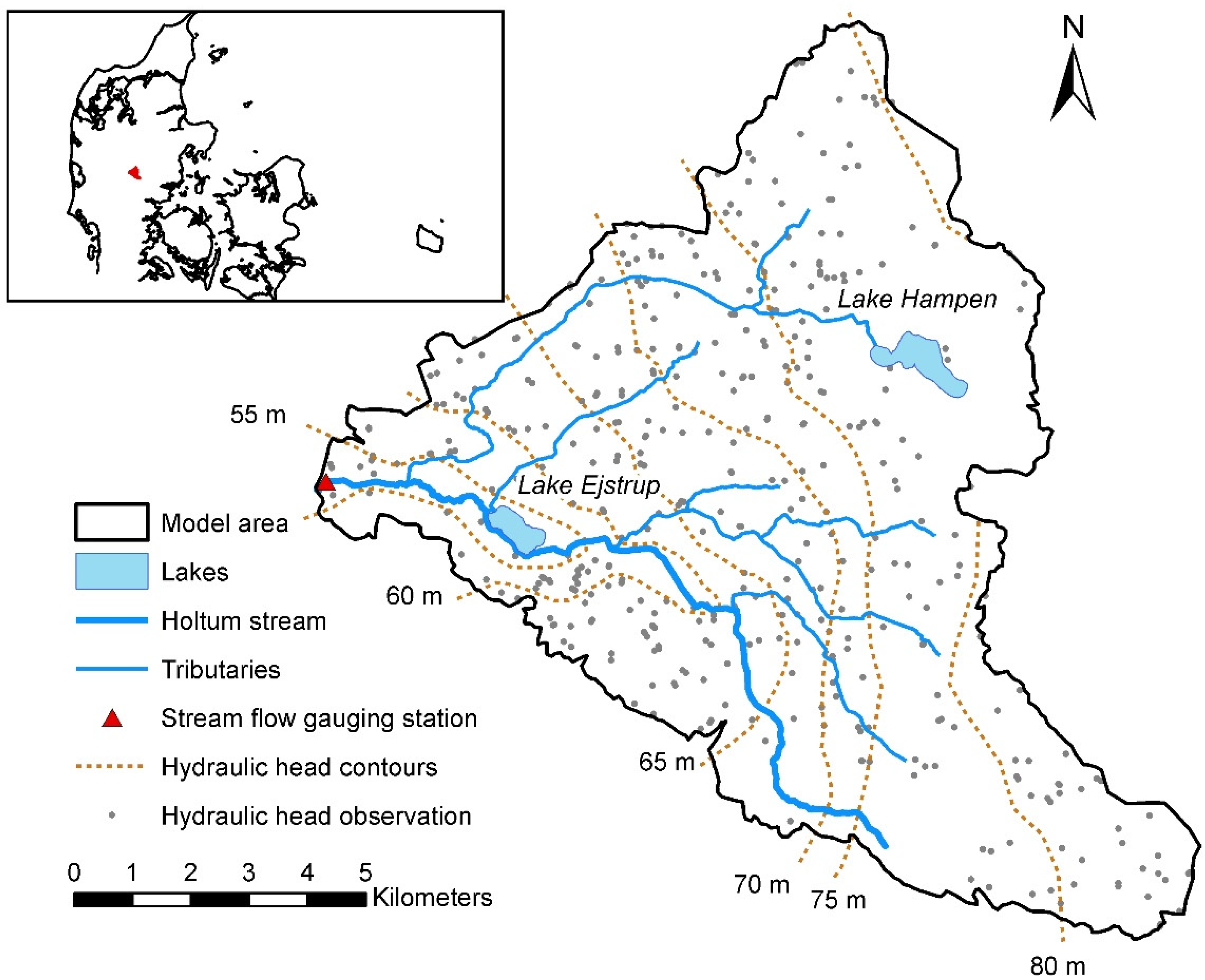
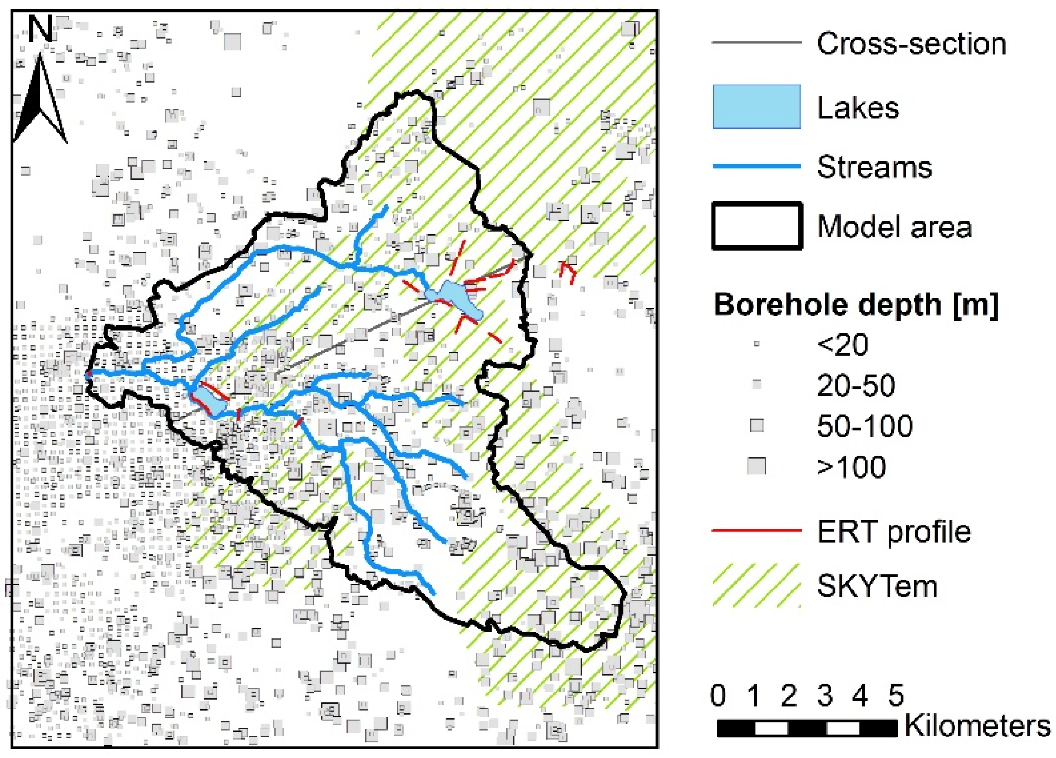
2.1. Study Area and Setting
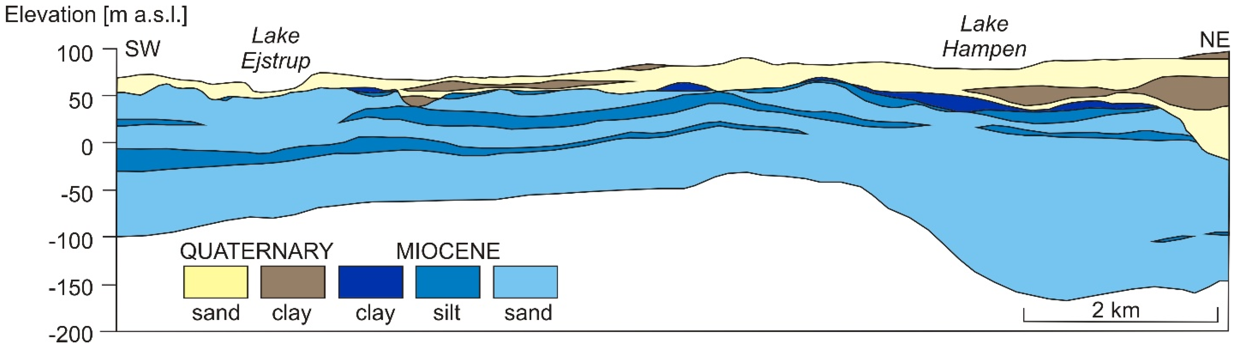
2.2. Geological Setting
2.3. Numerical Modeling
2.3.1. Conceptual Model
2.3.2. Model Calibration
3. Results
3.1. Geology
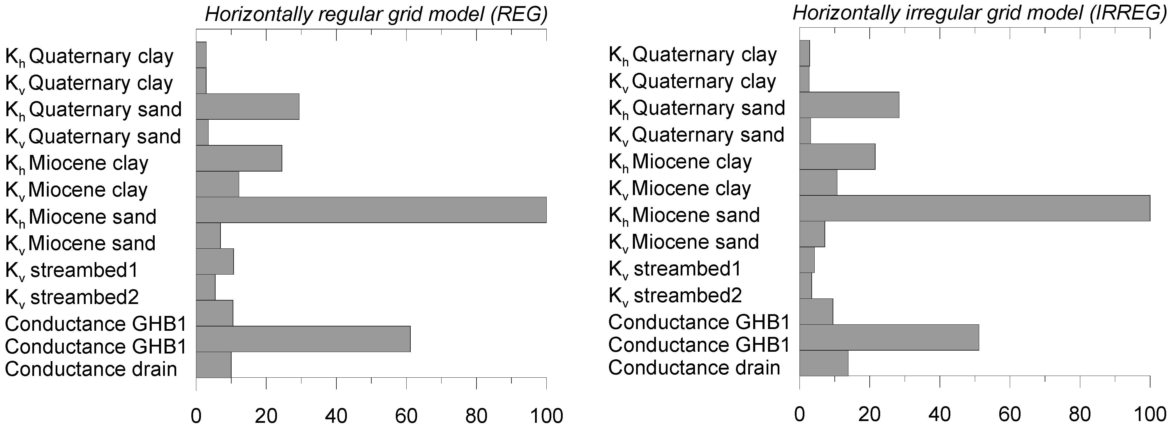
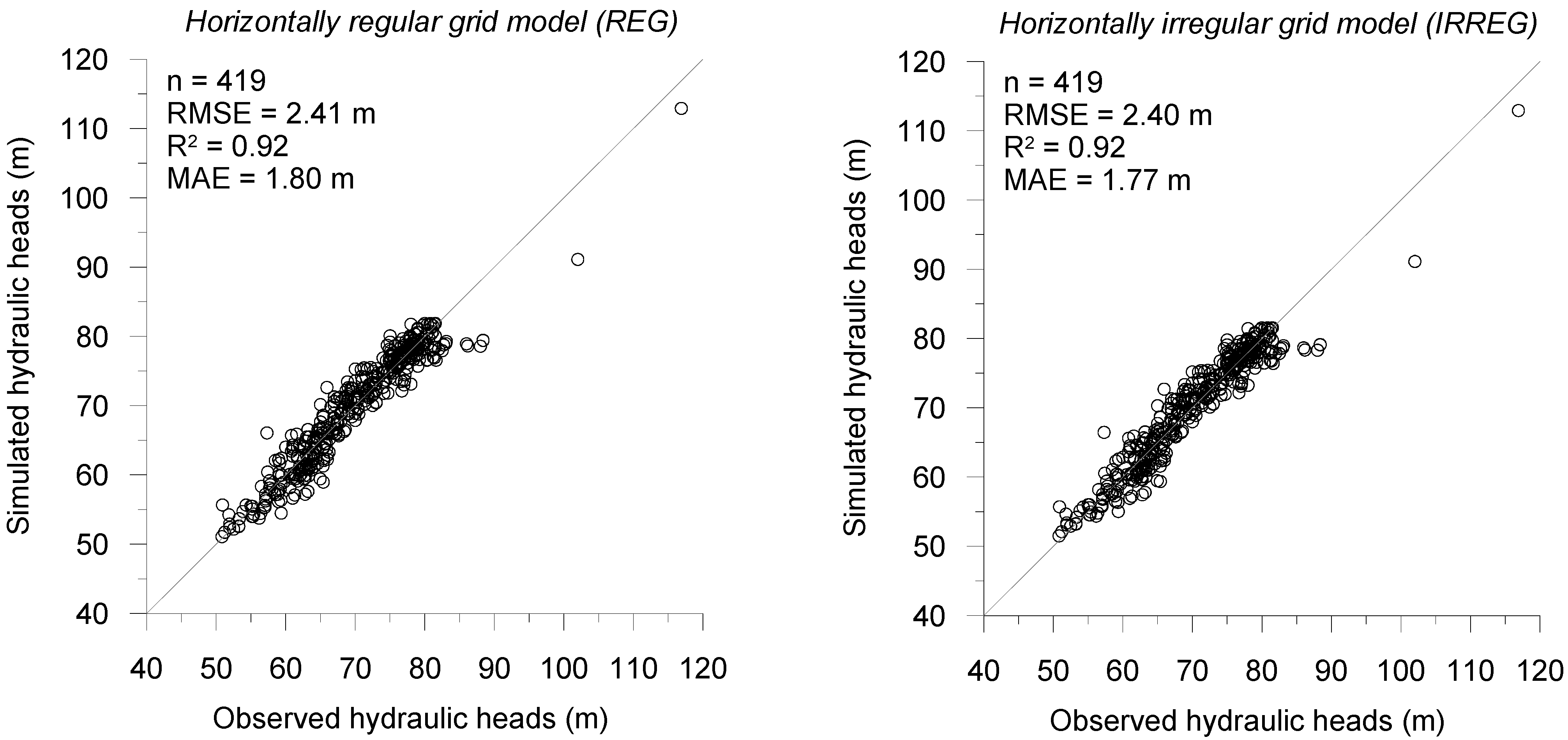
3.2. Model Calibration
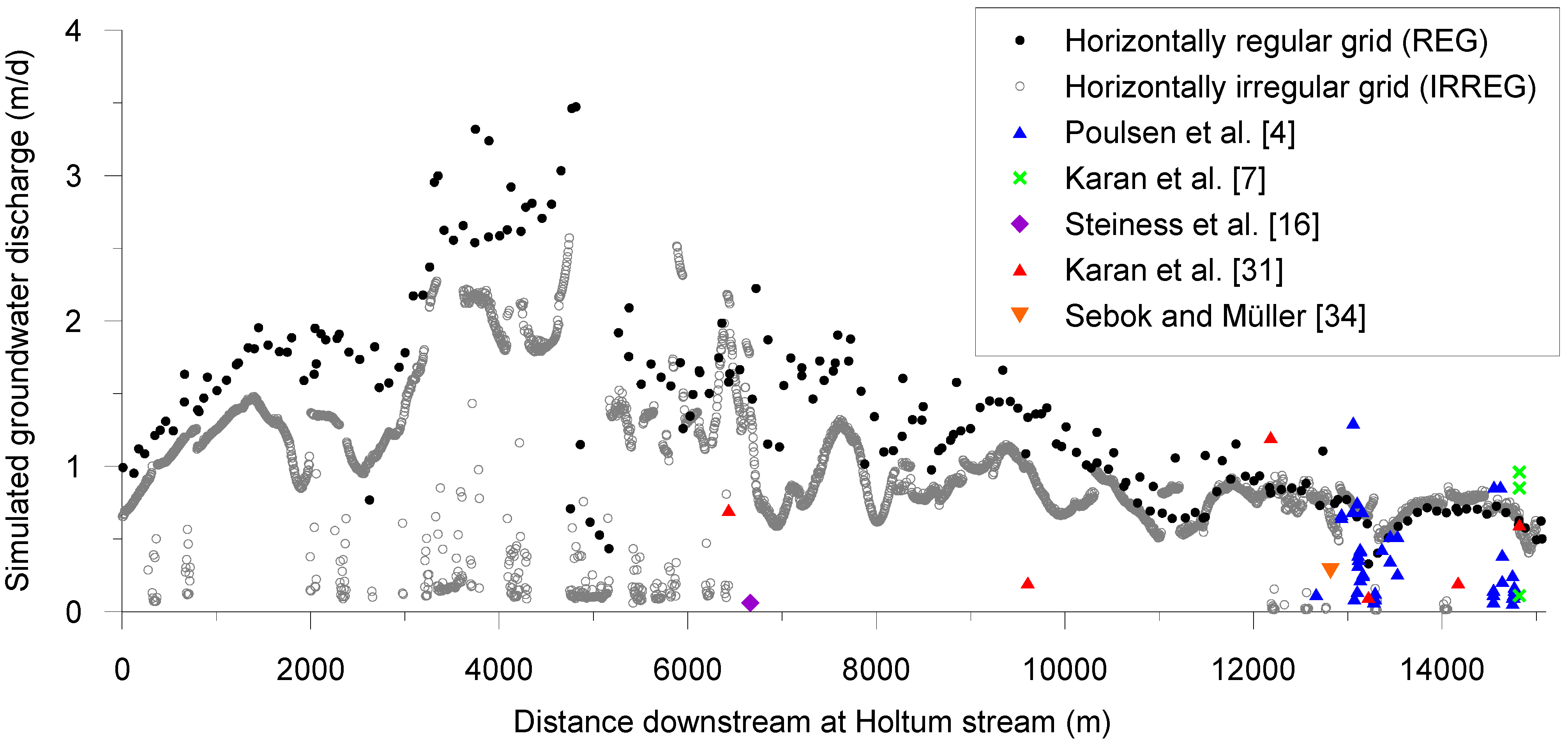
3.3. Stream Flow Contribution and Groundwater-Surface Water Exchange
4. Discussions
4.1. Parameter Calibration
4.2. Streamflow Contribution of Flow Balance Components
4.3. GW-SW Exchange Fluxes
5. Conclusions
Author Contributions
Funding
Institutional Review Board Statement
Informed Consent Statement
Data Availability Statement
Conflicts of Interest
References
- Constantz, J. Heat as a tracer to determine streambed water exchanges. Water Resour. Res. 2008, 44. [Google Scholar] [CrossRef]
- Karan, S.; Engesgaard, P.; Rasmussen, J. Dynamic streambed fluxes during rainfall-runoff events. Water Resour. Res. 2014, 50, 2293–2311. [Google Scholar] [CrossRef]
- Poulsen, J.R.; Sebok, E.; Duque, C.; Tetzlaff, D.; Engesgaard, P.K. Detecting groundwater discharge dynamics from point-to-catchment scale in a lowland stream: Combining hydraulic and tracer methods. Hydrol. Earth Syst. Sci. 2015, 19, 1871–1886. [Google Scholar] [CrossRef] [Green Version]
- Sebok, E.; Duque, C.; Engesgaard, P.; Boegh, E. Spatial variability in streambed hydraulic conductivity of contrasting stream morphologies: Channel bend and straight channel. Hydrol. Process. 2015, 29, 458–472. [Google Scholar] [CrossRef]
- Schilling, O.S.; Cook, P.G.; Brunner, P. Beyond Classical Observations in Hydrogeology: The Advantages of Including Exchange Flux, Temperature, Tracer Concentration, Residence Time, and Soil Moisture Observations in Groundwater Model Calibration. Rev. Geophys. 2019, 57, 146–182. [Google Scholar] [CrossRef] [Green Version]
- Kidmose, J.; Engesgaard, P.; Nilsson, B.; Laier, T.; Looms, M.C. Spatial Distribution of Seepage at a Flow-Through Lake: Lake Hampen, Western Denmark. Vadose Zone J. 2011, 10, 110–124. [Google Scholar] [CrossRef]
- Karan, S.; Engesgaard, P.; Looms, M.C.; Laier, T.; Kazmierczak, J. Groundwater flow and mixing in a wetland–stream system: Field study and numerical modeling. J. Hydrol. 2013, 488, 73–83. [Google Scholar] [CrossRef]
- Rahimi, M.; Essaid, H.I.; Wilson, J.T. The role of dynamic surface water-groundwater exchange on streambed denitrification in a first-order, low-relief agricultural watershed. Water Resour. Res. 2015, 51, 9514–9538. [Google Scholar] [CrossRef]
- Munz, M.; Oswald, S.E.; Schmidt, C. Coupled Long-Term Simulation of Reach-Scale Water and Heat Fluxes Across the River-Groundwater Interface for Retrieving Hyporheic Residence Times and Temperature Dynamics. Water Resour. Res. 2017, 53, 8900–8924. [Google Scholar] [CrossRef]
- Williams, M.R.; King, K.W.; Fausey, N.R. Contribution of tile drains to basin discharge and nitrogen export in a headwater agricultural watershed. Agric. Water Manag. 2015, 158, 42–50. [Google Scholar] [CrossRef]
- Ford, W.I.; King, K.; Williams, M.R. Upland and in-stream controls on baseflow nutrient dynamics in tile-drained agroecosystem watersheds. J. Hydrol. 2018, 556, 800–812. [Google Scholar] [CrossRef]
- Goeller, B.C.; Febria, C.M.; Warburton, H.J.; Hogsden, K.L.; Collins, K.E.; Devlin, H.S.; Harding, J.S.; McIntosh, A.R. Springs drive downstream nitrate export from artificially-drained agricultural headwater catchments. Sci. Total Environ. 2019, 671, 119–128. [Google Scholar] [CrossRef] [PubMed]
- Rosenbom, A.E.; Karan, S.; Badawi, N.; Gudmundsson, L.; Hansen, C.H.; Nielsen, C.B.; Plauborg, F.; Olsen, P. The Danish Pesticide Leaching Assessment Programme: Monitoring Results, May 1999–June 2019; Geological Survey of Denmark and Greenland: Copenhagen, Denmark, 2020.
- King, K.W.; Fausey, N.R.; Williams, M.R. Effect of subsurface drainage on streamflow in an agricultural headwater watershed. J. Hydrol. 2014, 519, 438–445. [Google Scholar] [CrossRef]
- Hansen, A.L.; Jakobsen, R.; Refsgaard, J.C.; Højberg, A.L.; Iversen, B.V.; Kjærgaard, C. Groundwater dynamics and effect of tile drainage on water flow across the redox interface in a Danish Weichsel till area. Adv. Water Resour. 2019, 123, 23–39. [Google Scholar] [CrossRef]
- Steiness, M.; Jessen, S.; Spitilli, M.; van’t Veen, S.G.; Højberg, A.L.; Engesgaard, P. The role of management of stream–riparian zones on subsurface–surface flow components. Water 2019, 11, 1905. [Google Scholar] [CrossRef] [Green Version]
- Steiness, M.; Jessen, S.; van’t Veen, S.G.; Kofod, T.; Højberg, A.L.; Engesgaard, P. Nitrogen-Loads to Streams: Importance of Bypass Flow and Nitrate Removal Processes. J. Geophys. Res. Biogeosciences 2021, 126, e2020JG006111. [Google Scholar] [CrossRef]
- King, K.W.; Williams, M.R.; Macrae, M.L.; Fausey, N.R.; Frankenberger, J.; Smith, D.R.; Kleinman, P.J.A.; Brown, L.C. Phosphorus Transport in Agricultural Subsurface Drainage: A Review. J. Environ. Qual. 2015, 44, 467–485. [Google Scholar] [CrossRef] [Green Version]
- De Schepper, G.; Therrien, R.; Refsgaard, J.C.; Hansen, A.L. Simulating coupled surface and subsurface water flow in a tile-drained agricultural catchment. J. Hydrol. 2015, 521, 374–388. [Google Scholar] [CrossRef]
- Sonnenborg, T.O.; Scharling, P.B.; Hinsby, K.; Rasmussen, E.S.; Engesgaard, P. Aquifer Vulnerability Assessment Based on Sequence Stratigraphic and 39 Ar Transport Modeling. Ground Water 2015, 54, 214–230. [Google Scholar] [CrossRef]
- Vervloet, L.S.; Binning, P.J.; Børgesen, C.D.; Højberg, A.L. Delay in catchment nitrogen load to streams following restrictions on fertilizer application. Sci. Total Environ. 2018, 627, 1154–1166. [Google Scholar] [CrossRef]
- Ranalli, A.J.; Macalady, D.L. The importance of the riparian zone and in-stream processes in nitrate attenuation in undisturbed and agricultural watersheds—A review of the scientific literature. J. Hydrol. 2010, 389, 406–415. [Google Scholar] [CrossRef]
- Panday, S.; Langevin, C.D.; Niswonger, R.G.; Ibaraki, M.; Hughes, J.D. MODFLOW–USG version 1: An unstructured grid version of MODFLOW for simulating groundwater flow and tightly coupled processes using a control volume finite-difference formulation. Tech. Methods 2013. [Google Scholar] [CrossRef]
- Jensen, J.K.; Engesgaard, P. Nonuniform Groundwater Discharge across a Streambed: Heat as a Tracer. Vadose Zone J. 2011, 10, 98–109. [Google Scholar] [CrossRef]
- Karan, S.; Kidmose, J.; Engesgaard, P.; Nilsson, B.; Frandsen, M.; Ommen, D.; Flindt, M.R.; Andersen, F.Ø.; Pedersen, O. Role of a groundwater–lake interface in controlling seepage of water and nitrate. J. Hydrol. 2014, 517, 791–802. [Google Scholar] [CrossRef]
- Hajati, M.C.; Frandsen, M.; Pedersen, O.; Nilsson, B.; Duque, C.; Engesgaard, P. Flow reversals in groundwater–lake interactions: A natural tracer study using δ18O. Limnologica 2018, 68, 26–35. [Google Scholar] [CrossRef]
- Geological Survey of Denmark and Greenland (GEUS). National Well Database (Jupiter). Available online: https://eng.geus.dk/products-services-facilities/data-and-maps/national-well-database-jupiter (accessed on 7 June 2021).
- Rasmussen, E.S.; Dybkjær, K.; Piasecki, S. Lithostratigraphy of the Upper Oligocene—Miocene succession of Denmark. Geol. Surv. Den. Greenl. Bull. 2010, 22, 1–92. [Google Scholar] [CrossRef] [Green Version]
- Houmark-Nielsen, M. Pleistocene Glaciations in Denmark: A Closer Look at Chronology, Ice Dynamics and Landforms. Dev. Quat. Sci. 2011, 15, 47–58. [Google Scholar] [CrossRef]
- Niswonger, R.G.; Prudic, D.E. Documentation of the Streamflow-Routing (SFR2) Package to Include Unsaturated Flow Beneath Streams—A Modification to SFR1. Tech. Methods 2005. [Google Scholar] [CrossRef] [Green Version]
- Karan, S.; Sebok, E.; Engesgaard, P. Air/water/sediment temperature contrasts in small streams to identify groundwater seepage locations. Hydrol. Process. 2017, 31, 1258–1270. [Google Scholar] [CrossRef]
- Doherty, J. Calibration and Uncertainty Analysis for Complex Environmental Models; Watermark Numerical Computing: Brisbane, Australia, 2015. [Google Scholar]
- Henriksen, H.J.; Troldborg, L.; Sonnenborg, T.; Højberg, A.L.; Stisen, S.; Kidmose, J.B.; Refsgaard, J.C. Hydrologisk Geovejledning—God Praksis i Hydrologisk Modellering (Hydrological Geoguide—Best Practice in Hydrological Modeling). Guide 2017/1; De Nationale Geologiske Undersøgelser for Danmark og Grønland—GEUS (Geological Survey of Denmark and Greenland): Copenhagen, Denmark, 2017; p. 130.
- Sebok, E.; Müller, S. The effect of sediment thermal conductivity on vertical groundwater flux estimates. Hydrol. Earth Syst. Sci. 2019, 23, 3305–3317. [Google Scholar] [CrossRef] [Green Version]
- Stisen, S.; Ondracek, M.; Troldborg, L.; Schneider, R.J.M.; van Til, M.J. National Vandressource Model. Modelopstilling og kalibrering af DK-model 2019. In Danmarks Og Grønlands Geologiske Undersøgelse Rapport 2019/31; Geological Survey of Denmark and Greenland: Copenhagen, Denmark, 2019. [Google Scholar]
- Hill, A.R. Nitrate Removal in Stream Riparian Zones. J. Environ. Qual. 1996, 25, 743–755. [Google Scholar] [CrossRef]
- Hill, A.R. Groundwater nitrate removal in riparian buffer zones: A review of research progress in the past 20 years. Biogeochemistry 2019, 143, 347–369. [Google Scholar] [CrossRef]
- Anderson, M.P.; Woessner, W.W.; Hunt, R.J. Applied Groundwater Modeling: Simulation of Flow and Advective Transport; Academic Press: Cambridge, MA, USA, 2015. [Google Scholar]
- Hansen, A.L.; Refsgaard, J.C.; Christensen, B.S.B.; Jensen, K.H. Importance of including small-scale tile drain discharge in the calibration of a coupled groundwater-surface water catchment model. Water Resour. Res. 2013, 49, 585–603. [Google Scholar] [CrossRef] [Green Version]


| Model Conceptualization | Parameter | Optimized Value | Lower 95% Confidence | Upper 95% Confidence | Units |
|---|---|---|---|---|---|
| Horizontally regular grid (REG) | Kh Quaternary sand | 32 | 14 | 71 | (m/d) |
| Kh Miocene sand | 16 | 14 | 19 | (m/d) | |
| Kh Miocene clay | 0.065 | 0.032 | 0.13 | (m/d) | |
| Kv streambed | 0.73 | 0.39 | 1.3 | (m/d) | |
| Conductance drain | 0.078 | 0.00019 | 32 | (1/d) | |
| Conductance general head | 0.032 | 0.0086 | 0.12 | (1/d) | |
| Horizontally irregular grid (IRREG) | Kh Quaternary sand | 30 | 14 | 64 | (m/d) |
| Kh Miocene sand | 17 | 14 | 20 | (m/d) | |
| Kh Miocene clay | 0.067 | 0.032 | 0.14 | (m/d) | |
| Kv streambed | 0.59 | 0.31 | 1.2 | (m/d) | |
| Conductance drain * | 0.05 | - | - | (1/d) | |
| Conductance general head | 0.014 | 0.0061 | 0.030 | (1/d) |
| Flow Budget | Horizontally Regular Grid (REG) | Horizontally Irregular Grid (IRREG) |
|---|---|---|
| Stream flow | 80.5 | 63.0 |
| Drainage | 12.5 | 30.9 |
| General head boundary | 7.0 | 6.1 |
Publisher’s Note: MDPI stays neutral with regard to jurisdictional claims in published maps and institutional affiliations. |
© 2021 by the authors. Licensee MDPI, Basel, Switzerland. This article is an open access article distributed under the terms and conditions of the Creative Commons Attribution (CC BY) license (https://creativecommons.org/licenses/by/4.0/).
Share and Cite
Karan, S.; Jacobsen, M.; Kazmierczak, J.; Reyna-Gutiérrez, J.A.; Breum, T.; Engesgaard, P. Numerical Representation of Groundwater-Surface Water Exchange and the Effect on Streamflow Contribution Estimates. Water 2021, 13, 1923. https://doi.org/10.3390/w13141923
Karan S, Jacobsen M, Kazmierczak J, Reyna-Gutiérrez JA, Breum T, Engesgaard P. Numerical Representation of Groundwater-Surface Water Exchange and the Effect on Streamflow Contribution Estimates. Water. 2021; 13(14):1923. https://doi.org/10.3390/w13141923
Chicago/Turabian StyleKaran, Sachin, Martin Jacobsen, Jolanta Kazmierczak, José A. Reyna-Gutiérrez, Thomas Breum, and Peter Engesgaard. 2021. "Numerical Representation of Groundwater-Surface Water Exchange and the Effect on Streamflow Contribution Estimates" Water 13, no. 14: 1923. https://doi.org/10.3390/w13141923