
Prediction of the Cavitation over a Twisted Hydrofoil Considering the Nuclei Fraction Sensitivity at 4000 m Altitude Level

1
School of Water Resources and Civil Engineering, Tibet Agriculture & Animal Husbandry University, Linzhi 860000, China
2
College of Water Resources and Civil Engineering, China Agricultural University, Beijing 100083, China
3
Beijing Engineering Research Center of Safety and Energy Saving Technology for Water Supply Network System, China Agricultural University, Beijing 100083, China
*
Author to whom correspondence should be addressed.
Water 2021, 13(14), 1938; https://doi.org/10.3390/w13141938
Submission received: 9 June 2021
/
Revised: 11 July 2021
/
Accepted: 11 July 2021
/
Published: 13 July 2021
(This article belongs to the Section Hydraulics and Hydrodynamics)
Abstract
:Cavitation phenomenon is important in hydraulic turbomachineries. With the construction of pumping stations and hydro power stations on plateau, the influence of nuclei fraction on cavitation becomes important. As a simplified model, a twisted hydrofoil was used in this study to understand the cavitation behaviors on pump impeller blade and turbine runner blade at different altitude levels. The altitudes of 0 m, 1000 m, 2000 m, 3000 m and 4000 m were comparatively studied for simulating the plateau situation. Results show that the cavitation volume proportion fcav increases with the decreasing of cavitation coefficient Cσ. At a specific Cσ, high altitude and few nuclei will cause smaller size of cavitation. The smaller Cσ is, the higher the sensitivity Δfcav is. The larger Cσ is, the higher the relative sensitivity Δfcav* is. On the twisted foil, flow incidence angle increases from the sidewall to mid-span with the decreasing of the local minimum pressure. When Cσ is continually decreasing, the size of cavitation extends in spanwise, streamwise and thickness directions. The cavity is broken by the backward-jet flow when Cσ becomes small. A tail generates and the cavity becomes relatively unstable. This study will provide reference for evaluating the cavitation status of the water pumps and hydroturbines installed on a plateau with high altitude level.
1. Introduction
Cavitation is a commonly seen phenomenon in hydrodynamic turbomachinery cases such as pumps and hydroturbines [1,2,3]. It usually has bad influences including noise [4], vibration [5] and material damage [6]. For this reason, cavitating flow in hydraulic turbomachinery has been widely studied by researchers to understand its mechanism, behavior and influence. As a simplification of the blade of hydraulic turbomachinery, hydrofoil is usually used in the study of cavitation and cavitating flow. Arabnejad et al. [7] and Tao et al. [8] investigated the leading-edge cavitation over symmetric hydrofoils. Different types of leading-edge cavitation are discussed in detail. Dreyer et al. [9] and Guo et al. [10] used hydrofoil to have a better study of the tip-leakage cavitation of blade. Cavitation happening in the tip-leakage vortex was studied to help the anti-cavitation design of axial-flow hydraulic runners. Escaler et al. [11] and Melissaris et al. [12] used hydrofoil models to study the cavitation erosion behavior of hydraulic runner blades. The erosion risk can be well evaluated.
In these previous studies, cavitation on hydrofoil surfaces is mainly found related to the local flow separation and pressure drop [13]. Under different flow conditions, cavitation performs in different types. If the size of cavitation is small and flow is stable, the cavitation bubble will also stably attach on the surface [14]. If local flow is unstable and the size of cavitation becomes large, the cavitation bubble will move with flow as a cloudy cavitation [15]. Generally, the status of cavitation on impeller blade or hydrofoil is strongly related to the blade (foil) profile, local flow stability and the size of cavitation itself. As another important factor, the nuclei fraction will also affect the status of cavitation [16]. However, this factor is usually ignored, because the nuclei fraction in water medium has only a slight influence on cavitation.
Currently, more and more pumping stations and water power stations are constructed on plateau [17,18,19]. There are many stations built above 3000 m or even above 4000 m. Thus, the nuclei fraction in water medium is completely different from the situation in low-altitude area. It may have a strong influence on cavitating flow. As a robust and effective way in studying cavitation, the computational fluid dynamics (CFD) tool is widely applied especially for water pumps and hydroturbines [20,21,22,23,24]. Based on CFD, different cavitation models can be supplied to predict the cavitating two-phase flow. Currently, most of the popular cavitation models are based on the Rayleigh–Plesset equation [25], which describes the bubble dynamics under the influence of pressure field. Kubota et al. [26] built– a cavitation model based on the Rayleigh–Plesset equation to calculate the cavitation bubble size and vapor fraction. Considering the influence of compressibility and pressure pulsation caused by turbulence kinetic energy, Singhal et al. [27] supposed the full cavitation model as an improvement in the simulation of cavitating flow. Schnerr and Sauer [28] focused on the modeling of the mass transfer rate between gas phase and liquid phase. The Schnerr–Sauer model is built to treat the cavitating flow as a mixture of liquid and a large number of gas bubbles. Zwart, Gerber and Belamri [29] improved the cavitation prediction method based on the Kubota model. In the Zwart model, the volume fraction terms are corrected because gas volume will vary with the medium density. Kunz et al. [30] considered the difference between the form and collapse of cavitation bubble. They introduced the Kunz model, which describes the liquid–gas phase change and gas-liquid phase change in different ways. In general, all these models consider the influence of nuclei fraction on cavitation. Hence, it will be feasible to discuss the influence of nuclei fraction in simulating the cavitation at different altitude levels.
However, there is no article that analyzes the influence of nuclei fraction in simulating the cavitation in hydraulic turbomachineries. Cavitation in hydraulic turbomachinery is strongly relative to the internal complex flow regimes like vortex, back flow, jet-wake, stall-cells and other pressure drop cases [31]. In this case, a twisted hydrofoil [32] was used as a simplified case to have a sensitivity analysis of nuclei fraction in simulating the cavitation at different altitude levels. Considering the altitude of the Qinghai–Tibet Plateau, which is over 4000 m, the air pressure is strongly different from that in the low-altitude area [33]. According to Henry’s law, the nuclei fraction strongly varies from low-altitude area to a 4000 m plateau. This study will comparatively analyze the cavitation at high altitude level. With the nuclei fraction at 4000 m, the turbulent flow and development of cavitation over the twisted hydrofoil was analyzed in detail. It will provide a good reference for water pumps and hydroturbines for high-altitude levels considering the anti-cavitation issue.
2. Numerical Methods
2.1. Numerical Method for Turbulent Flow
Considering the strong adverse pressure gradient in the main flow region and the shear flow near the, the Shear Stress Transport (SST) model-based Detached Eddy Simulation (DES) method [34,35] is used as the numerical method for turbulent flow in CFD simulation. The k and ω equations of SST model can be written as follows:
where ρ is density, P is the turbulence production term, μ is dynamic viscosity, μt is eddy viscosity, σ is model constant, Cω is the turbulence dissipation term, F1 is the zonal blending function, lk−ω is called the turbulence scale that lk-ω = k1/2βkω, where βk is the model constant. The DES method uses a zonal treatment term that min(lk−ω, CDES·Lmesh), where Lmesh is the maximum mesh element dimension and CDES is a constant. When lk−ω is larger than CDES·Lmesh, Large Eddy Simulation will be activated. Otherwise, SST model is used in the Reynolds-averaged mode.
2.2. Cavitation Model
The Zwart model [29] is a widely used cavitation model in current CFD simulations of cavitating two-phase flow. It is based on the Rayleigh–Plesset bubble dynamic equation to describe the mass transfer. It has the advantage that the sensitivity of cavitation vapor volume due to density change is considered. The requirement of computational cost when reasonable is used for engineering simulations. Therefore, it is applied as the cavitation model in this case. The rate of mass transfer can be expressed as:
where pv is the saturation pressure, ρv is the vapor density, fvnuc is the nuclei volume fraction, RB is the nuclei average radius, Fe and Fc are coefficients of evaporization and condensation which are commonly Fe = 50 and Fc = 0.01.
2.3. Vapor Volume Fraction
According to Henry’s law, the gas dissolved as nuclei in liquid is proportional to the gas pressure over the liquid surface. Based on the data statistics on the Qinghai–Tibet Plateau [33], the atmosphere pressure Patm and altitude Halt have the approximate relationship as:
where Cd are constants that Cd1 = 1.013 × 10⁵, Cd2 = 1.259 × 101, Cd3 = 6.476 × 10⁻⁴. Based on Henry’s law, the nuclei volume fraction fvnuc will be different if the altitude Halt is different. The original fvnuc at Halt = 0 m is 5 × 10⁻⁴. In this case, the altitude conditions that Halt = 0 m, 1000 m, 2000 m, 3000 m and 4000 m are comparatively studied. Therefore, the values of fvnuc are listed in Table 1.
3. Case and Setup
3.1. Important Dimensionless Parameters
In this study, the hydrofoil case was discussed. To investigate the cavitating flow, two dimensionless parameters are defined as follows. Firstly, the fundamental parameter in the cavitation description is the cavitation coefficient Cσ:
where pv is the saturation pressure, pref and vref are reference pressure and velocity, respectively, which are usually measured at the upstream of hydrofoil, ρ is density. Therefore, Cσ can be adjusted by changing the value of pref. Secondly, the pressure coefficient Cp can be defined as:
where p is pressure. Therefore, the same Cσ values can be compared for different altitudes with considering that the altitude caused a difference on nuclei volume fraction fvnuc.
3.2. Flow Domain of Hydrofoil
In this study, the Delft Twist 11 hydrofoil [32,36] was used based on the NACA0009 profile. This symmetric NACA 4-digit foil profile can be expressed as follows:
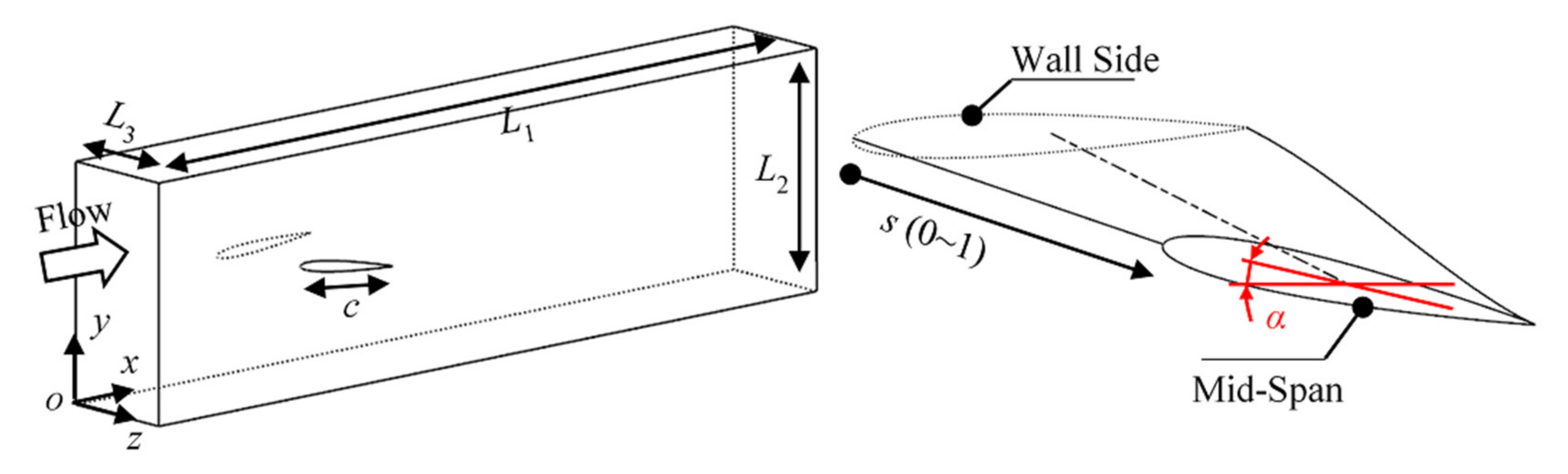
where c is the total camber length, X is the position along camber direction, Y is the thickness, Ym is the maximum thickness of foil. Parameter Ca and Cb are constants that Ca = 0.2, Cb1 = 0.2969, Cb2 = 0.126, Cb3 = 0.3516, Cb4 = 0.2843 and Cb5 = 0.1015. This twisted hydrofoil has a different installation angle α at a different span. It has the law of α as:
where s is the non-dimensionalized spanwise position against the chord length c and here 0 ≤ s ≤ 2. αm is the maximum installation angle at mid-span, which is 11 degrees. αw is the installation angle on the wall side, which is −2 degrees in this case.
The 3D flow domain around the twisted hydrofoil is shown in Figure 1, which location in the Cartesian x-y-z coordinate is used for CFD simulation. As shown in Figure 2, c denotes the total chord length of the hydrofoil and c = 1.5 Lref, where Lref is 100 mm. The domain size is L1 = 10.5 Lref, L2 = 3.0 Lref and L3 = 1.5 Lref. The foil center locates 3.0 Lref downstream to the inlet. In this case, the domain is simplified as a half of the entire flow region that s = z/c is within 0~1.
3.3. CFD Setup
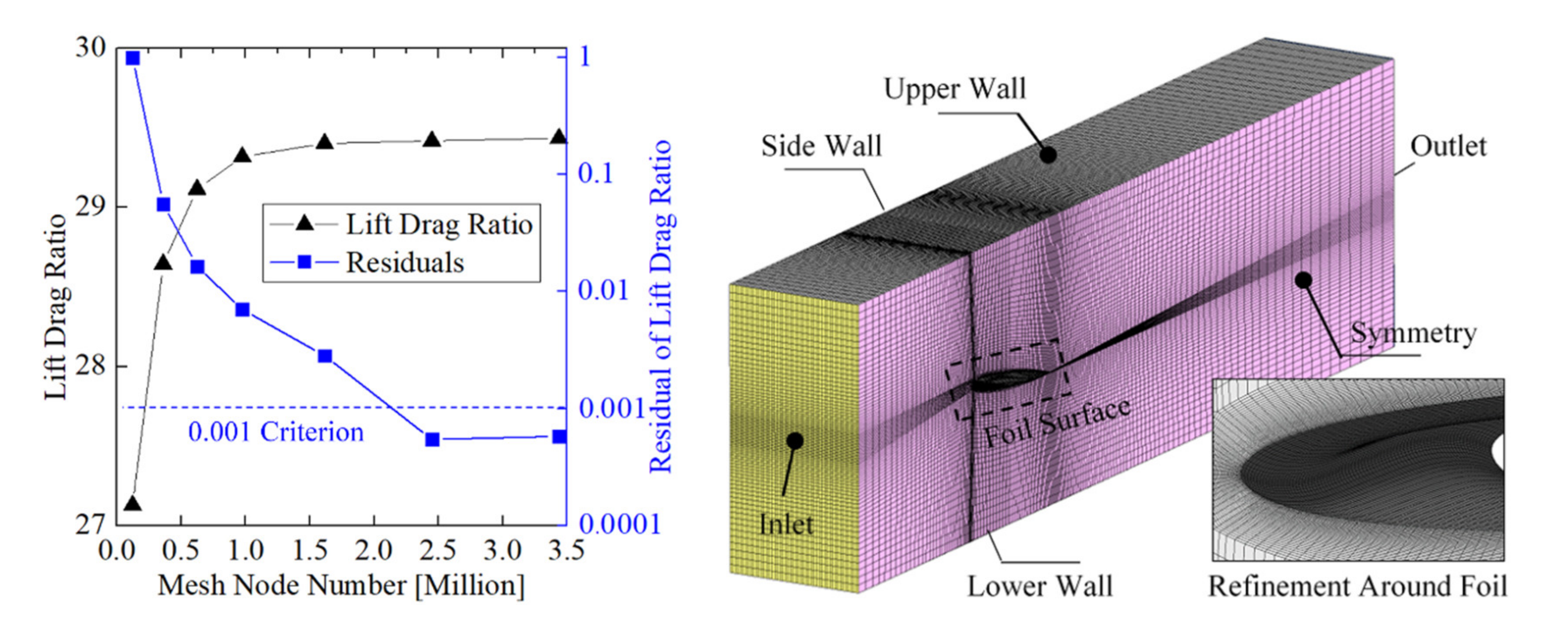
The CFD was conducted following the sequence of meshing, setting and solving. The mesh was independence-checked, as shown in Figure 2. The criterion is that the residual of lift/drag ratio is less than 0.001. The final mesh is in the structured type with 2,449,280 nodes and 2,380,744 hexahedral elements. Mesh in the near-wall region was controlled for wall-function where y+ was from 0.47 to 23.75. As introduced above, the DES method and Zwart cavitation model were used in this numerical study. The fluid is water at 20 °C. As indicated, boundary conditions are set on the domain including a velocity inlet, a pressure outlet, a symmetry boundary at mid-span, a no-slip wall on foil surface, slip wall boundaries on upper wall, lower wall and side wall. The inlet velocity vin is 6.97 m/s, which means that the Reynolds number Re is 1.05×10⁶. The reference location for Cp and Cσ is the inlet boundary. To have a better study of cavitation, the same Cσ situations are compared for different altitude levels. For a specific value of vin, the inlet–outlet pressure difference is almost unchanged. Thus, pref at inlet can be adjusted to an expectable value by setting a specific pressure value at outlet. Steady-state simulation is firstly conducted. It will converge after the RMS residual of momentum and continuity equation is less than 1 × 10⁻⁴ or finish after 1000 iterations. Transient simulation is conducted based on steady-state simulation. The total time is 1s and the time step is 1 × 10⁻⁵ s. The maximum iteration number for each time step is 10. The convergence criterion is also RMS residual less than 1 × 10⁻⁴.
4. Numerical-Experimental Verification
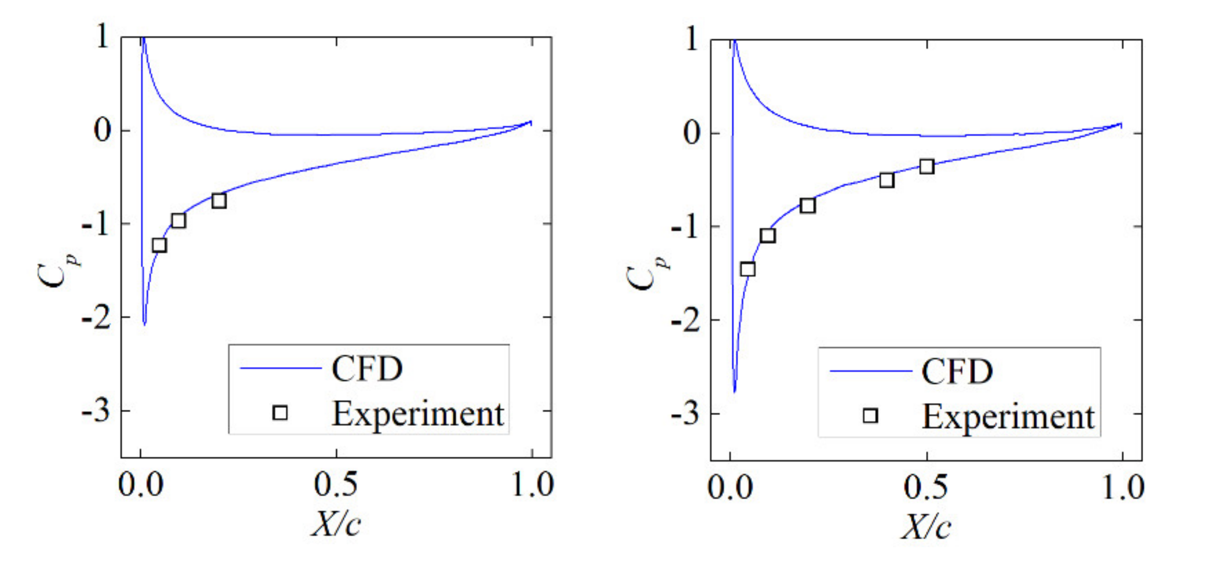
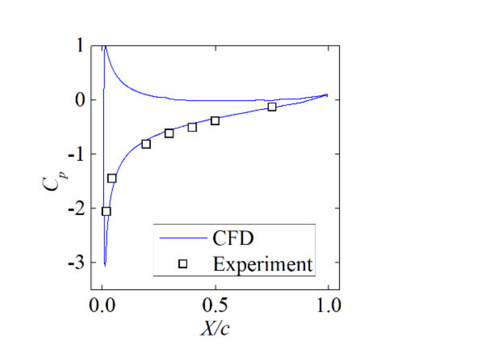
Before analyzing the CFD results, it is necessary to verify the simulation. Figure 3 shows the comparison of pressure coefficient Cp between CFD prediction and experimental data [12,36]. Three different spanwise positions in which s = 0.6, 0.8 and 1.0 are compared, especially focusing on the low-pressure side where cavitation usually occurs. The CFD predicted Cp curves are accurate on the three spanwise surfaces. The CFD simulation can be used for further analyses of the cavitating flow in the following sections.
5. Cavitation Vapor Proportion at Different Altitudes
5.1. Variation Law
To study the sensitivity of nuclei fraction at different altitudes Halt, the cavitation vapor proportion fcav in the fluid domain is defined as:
where Vcav is the cavitation vapor volume and Vfluid is the fluid domain volume.
Figure 4 shows the comparison of cavitation vapor proportion fcav among different Halt at different Cσ. With the decreasing of Cσ from 2.713 to 1.071, fcav continually increases to a high level. The smaller Cσ is, the quicker fcav increases. It represents the increasing of cavitation vapor in the entire fluid domain. However, there are differences among different Halt situations. Figure 5 shows the cavitation vapor proportion among different Halt at specific Cσ values. The tendency is similar in all the 9 situations that fcav decreases with the increasing of the Halt level.
5.2. Sensitivity Analysis
Because the size of cavitation is different at different Halt, it is necessary to analyze the sensitivity of fcav on Halt and fvnuc. The difference between maximum and minimum fcav among different Halt at a specific Cσ is defined as the sensitivity Δfcav. For a better comparison, the relative sensitivity Δfcav* is defined as:
where fcava is the average vapor proportion of all the 5 Halt situations.
Figure 6 shows the sensitivity analysis of fcav at different Cσ. The Halt-average vapor proportion fcava shows the same variation tendency as in Figure 4. fcava increases with the decreasing of Cσ. The sensitivity Δfcav has almost the similar tendency of fcava. The smaller Cσ is, the greater the difference is among different altitudes. However, there is a special local peak region when Δfcav drops to a low level around Cσ = 1.8. It means that the difference between maximum and minimum fcav is locally higher.
When the size of cavitation is small at high Cσ, the absolute difference of fcav among different Halt is also small. Therefore, it is necessary to compare the variation of relative sensitivity Δfcav*. As shown, the tendency is completely different. It is in a W-shape with two slowly variating regions and two rapidly rising regions, as indicated. The first rapidly rising region is about Cσ = 1.5~1.9. The secondly rapidly rising region is about Cσ = 2.5~2.7. Generally, when the size of cavitation is small, the relative sensitivity Δfcav* is higher. In the high altitude plateau area, it is necessary to consider the influence of altitude level on cavitation inception.
6. Flow Behaviors Considering Altitude Level
6.1. Pressure Distribution Law on Foil Surface
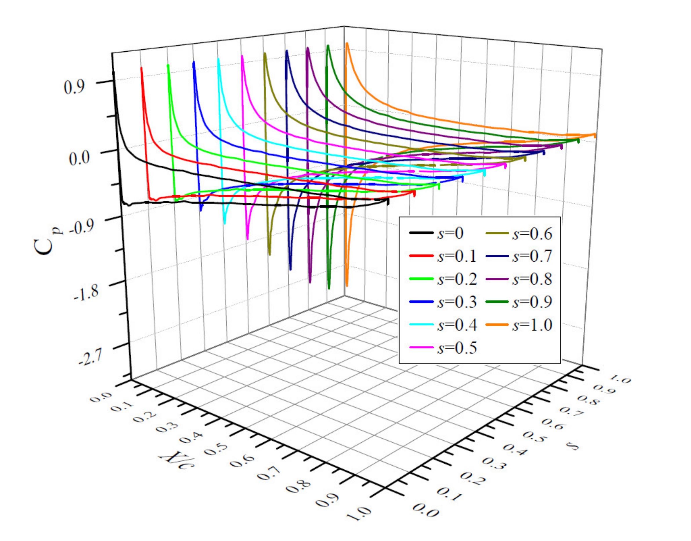
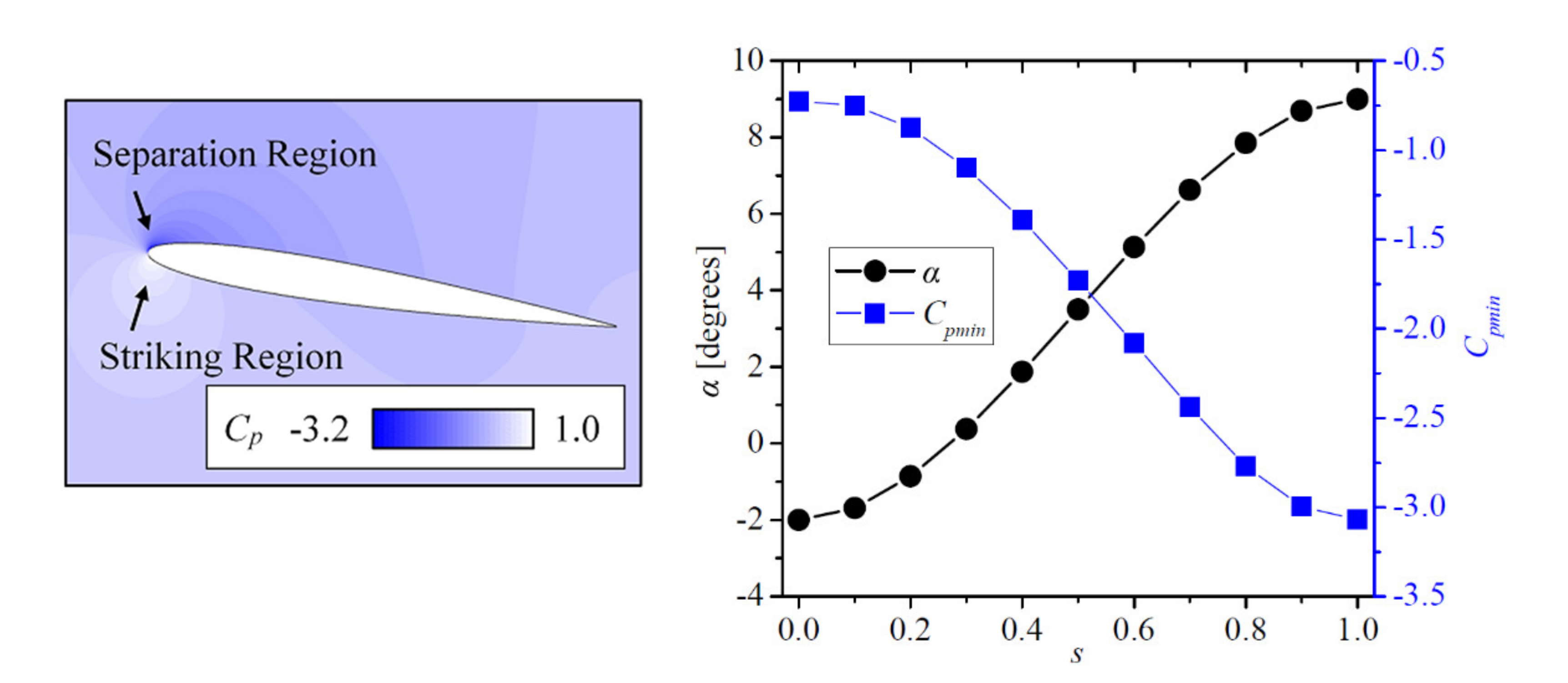
After analyzing the influence of altitude level on the simulation of cavitating flow, it is necessary to study the flow behaviors around the hydrofoil. As is commonly known, cavitation on hydrofoil is strongly related to the pressure distribution. Figure 7 shows the distribution of pressure coefficient Cp on different spanwise positions (0 ≤ s ≤ 1) of foil without considering cavitation. The maximum pressure coefficient Cpmax is similar (about 1.0) for different s. This high pressure is because of the local flow striking on the foil lower surface, as shown in Figure 8. The minimum pressure coefficient Cpmin varies with s. The larger s is, the smaller Cpmin is. This is because of the local flow separation on the foil upper surface, as is also shown in Figure 8.
To have a better comparison, Figure 8 shows the minimum pressure coefficient Cpmin and installation angle α at different spanwise s positions. There is a significant inverse relationship between Cpmin and α. The larger the installation angle is, the larger the flow incidence angle is. It indicates the stronger and stronger flow separation and pressure drop when incidence angle is increasing.
6.2. Turbulent Flow around Foil
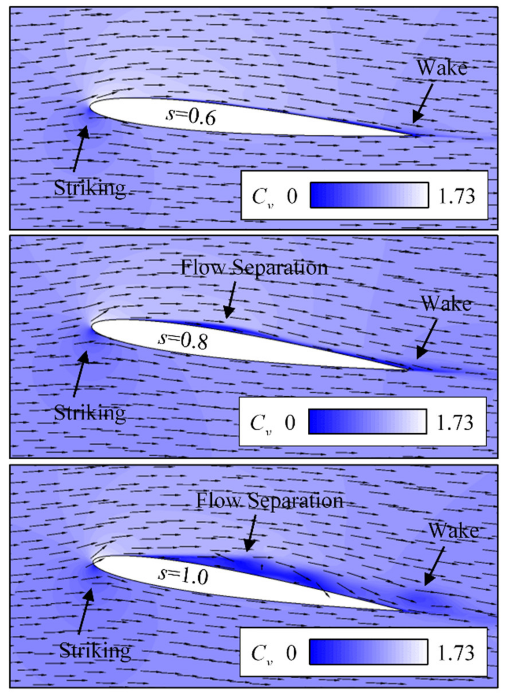
To have a better understanding of the pressure drop, Figure 9 shows the velocity coefficient Cv at different spanwise s positions with indication of vectors. The uniformed velocity Cv is defined as:
where v is velocity and vin is the velocity at inlet.
At s = 0.6, installation angle α is about 5.13 degrees. Flow attaches well on the foil surface. There are two typical low Cv regions. Firstly, it is the local flow striking region on the leading-edge on the foil lower surface. Secondly, it is the wake region downstream to the foil trailing-edge. At s = 0.8, installation angle α increases to about 7.86 degrees. An obvious flow separation region occurs on the foil upper surface with low Cv. The leading-edge striking region and the trailing-edge wake region are wider. At s = 1.0 (mid-span), installation angle α increases to 9 degrees, which is relatively large. It is obvious that the flow separation region on the foil upper surface is much wider. The leading-edge striking region and the trailing-edge wake region are also wider.
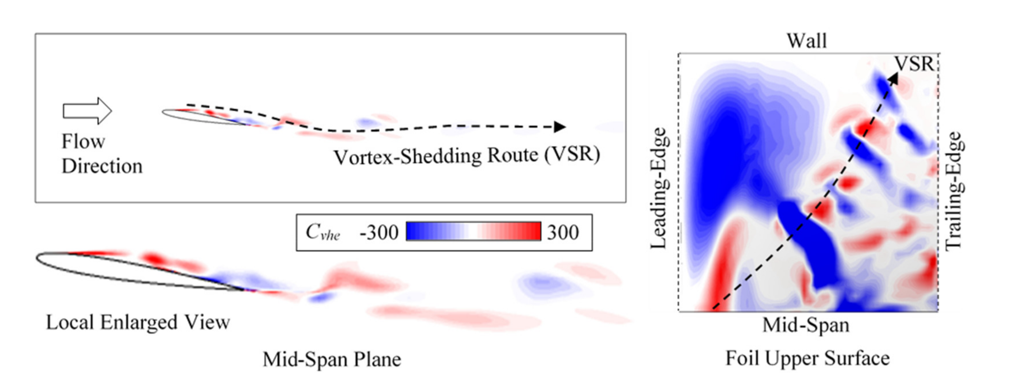
Considering the flow separation and sudden pressure drop at s = 1.0 (mid-span), it is necessary to analyze the local vortex shedding pattern, especially on the foil upper surface. In this case, the velocity helicity Hv is used [37]. It can be non-dimensionalized to the velocity helicity coefficient Cvhe by:
where g is the acceleration of gravity.
Figure 10 shows the velocity helicity coefficient Cvhe on the mid-span plane and foil upper surface. The vortex-shedding phenomenon can be seen with the indication of the vortex-shedding route (VSR). On the mid-span plane, obvious VSR can be found from leading-edge (LE), along the upper surface, to trailing-edge (TE) and towards downstream. On the foil upper surface, VSR is complex and mainly along the diagonal line from the LE-mid-span corner to the TE-wall corner. Generally speaking, local vortical flow moves along the slope of the twisted foil surface.
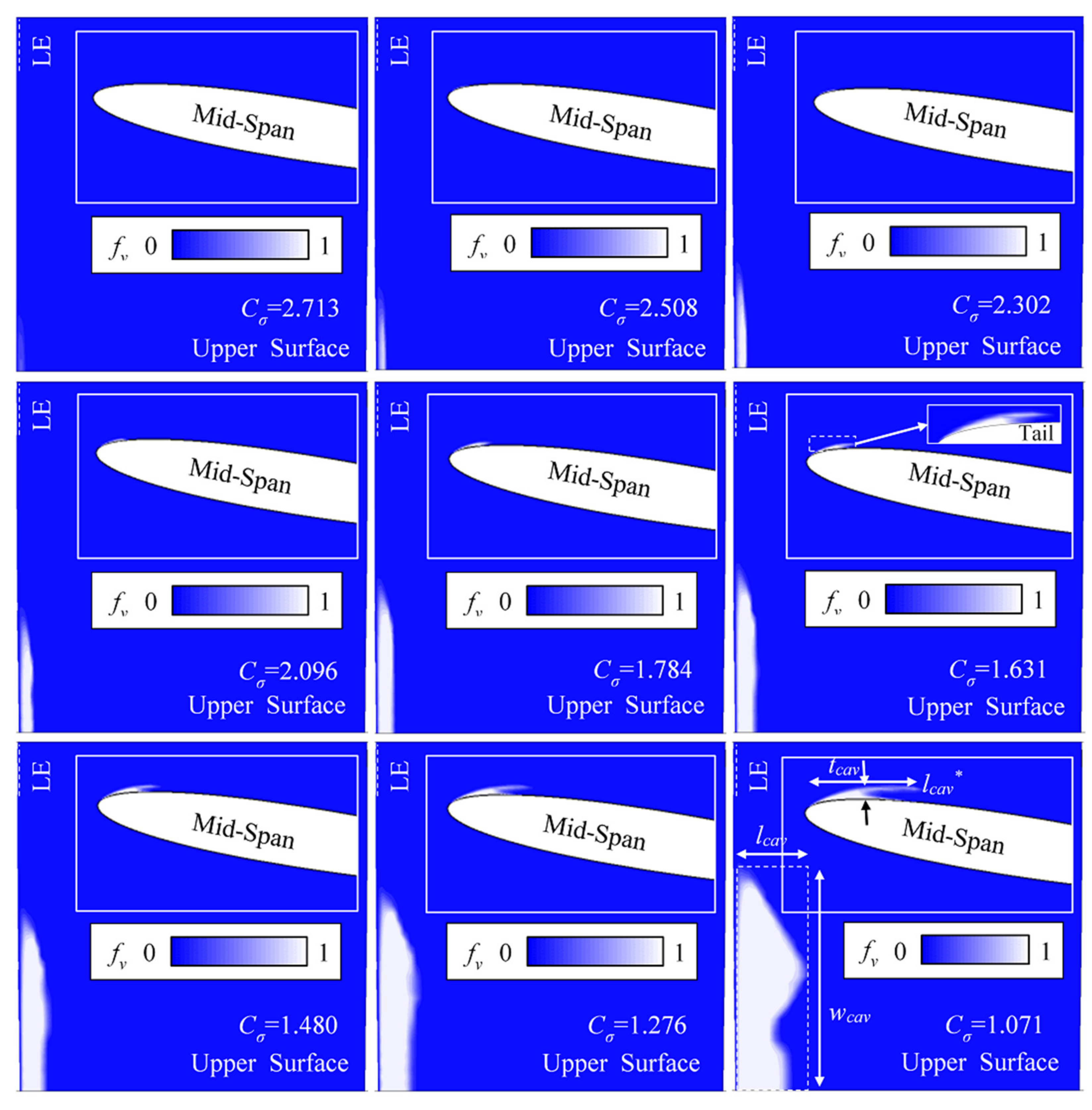
6.3. Development of Cavitation at Halt- = 4000 m
Considering the plateau environment that Halt = 4000 m and fvnuc = 3.01×10⁻⁴, the cavitating flow is simulated and analyzed in Figure 11. The development of cavitation is comparatively studied from Cσ = 2.713 to Cσ = 1.071. The scale of cavitation continually increases in different directions. Figure 11 mainly shows the region of cavitation covering on the foil upper surface. Leading-edge (LE) is on the left side. Two parameters are defined to have a quantitative comparison. One is the length of cavity-covered area lcav and another is the width of cavity-covered area wcav. Figure 11 also includes the mid-span view of cavitation. Two parameters are defined in this view. One is the maximum thickness of cavity on mid-span tcav. Another is the total length of the attached part of the cavity on mid-span, which is denoted as lcav*. In general, lcav, wcav, tcav and lcav* increase with the decreasing of cavitation coefficient Cσ.
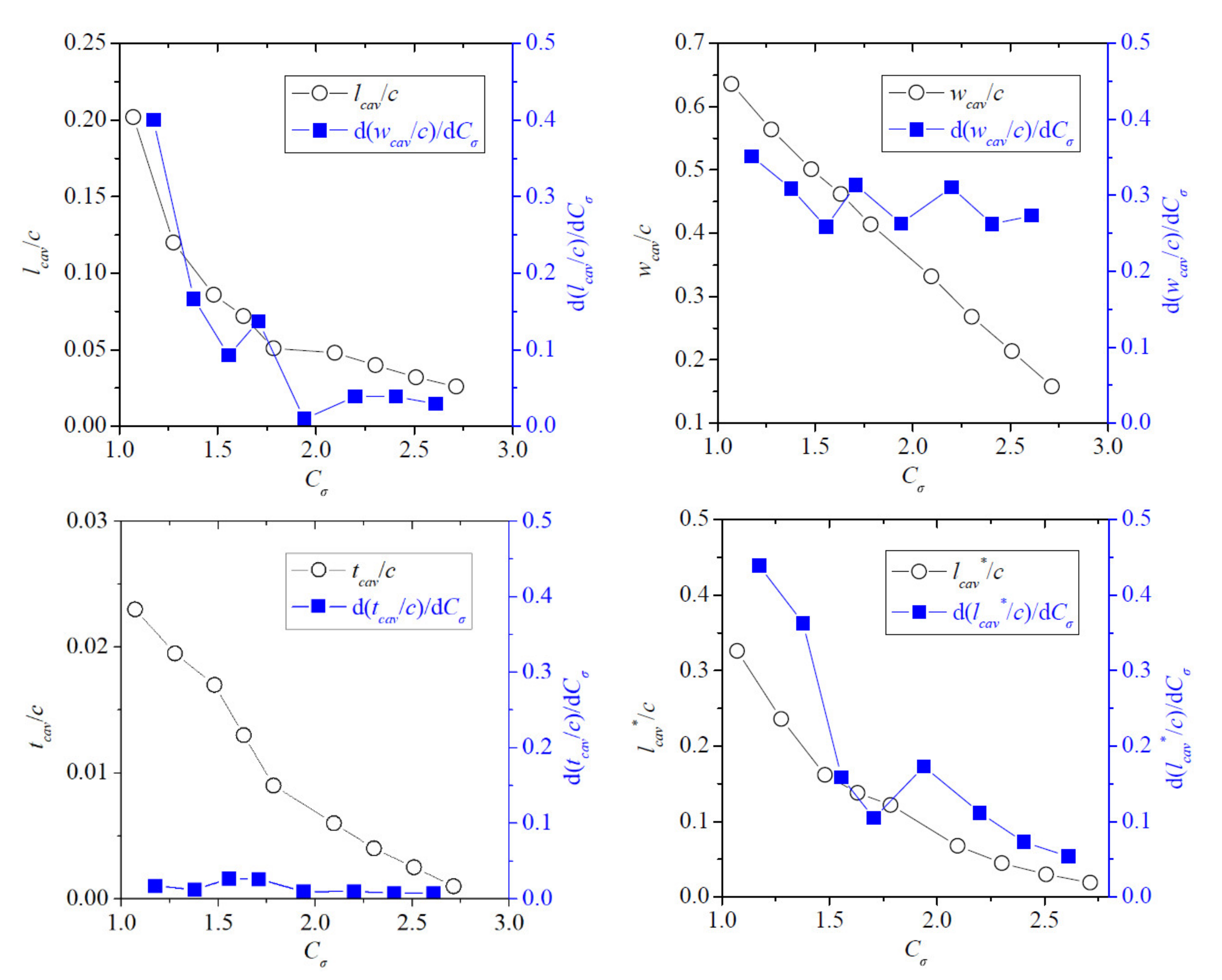
To have a better analysis, the variation of lcav, wcav, tcav and lcav* are compared in Figure 12. These four parameters are normalized against the foil chord length c. The growth rate dφ/dCσ is also analyzed between each two conditions.
For the length of cavity-covered area on foil upper surface lcav, the growth rate is relatively low, within Cσ = 2.173~1.784. The value of d(lcav/c)/dCσ is lower than 0.05. The value of lcav/c increases from about 0.026 to about 0.051. When Cσ is smaller than 1.784, the growth rate of lcav becomes much higher. The value of d(lcav/c)/dCσ is about 0.09~0.40. From Cσ = 1.784 to Cσ = 1.071, the value of lcav/c strongly increases from about 0.051 to 0.202. Cavity covers about 1/5 of the foil surface along x direction at Cσ = 1.071.
For the width of the cavity-covered area on foil upper surface wcav, the growth rate d(wcav/c)/dCσ is stable around 0.3. The increasing of wcav/c against Cσ is almost linear. From Cσ = 2.173 to Cσ = 1.071, wcav/c increases from about 0.158 to about 0.636. At Cσ = 1.071, cavity covers more than 3/5 of the half foil surface along the y direction.
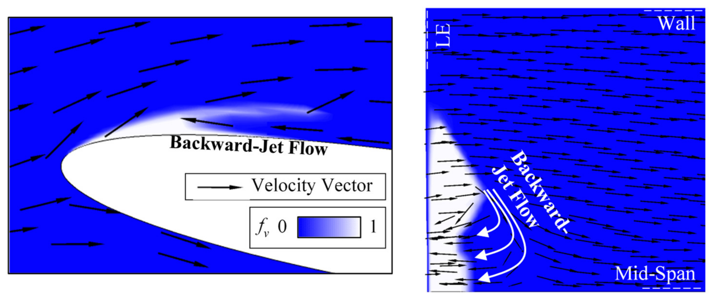
For the maximum thickness of cavity on mid-span tcav, the growth rate is relatively stable. The value of d(tcav/c)/dCσ is lower than 0.03. The increasing of tcav/c against Cσ is almost linear, except in a small range between 1.784 and 1.480. In this range, a special phenomenon occurs in which a tail can be seen on the profile of cavity. This is because of the backward-jet flow (indicated in Figure 13 as an example), and the cavity becomes much thicker. From Cσ = 2.173 to Cσ = 1.071, tcav/c increases from about 0.001 to about 0.023. This thickness (tcav/c = 0.023 at Cσ = 1.071) is about 1/4 of the maximum foil thickness.
For the total length of the attached part of cavity on mid-span lcav*, the growth rate is similar to lcav. From Cσ = 2.713 to Cσ = 1.480, the value of d(lcav*/c)/dCσ is lower than 0.2. The value of lcav* increases from about 0.019 to 0.162. From Cσ = 1.480 to Cσ = 1.071, the value of d(lcav*/c)/dCσ is 0.36~0.44. The value of lcav*/c obviously increases from about 0.162 to 0.326. Comparing with lcav, both the value and the growth rate of lcav* is higher. This is also because of the tail on cavity. The total length of cavity is bigger than the cavity length covering on foil surface.
Generally, cavitation on a twisted hydrofoil extends along the streamwise direction, spanwise direction and thickness direction with the decreasing of cavitation coefficient Cσ. When Cσ is at a higher level, the small-scale cavity is attached on foil surface. When Cσ becomes lower, cavity on large-incidence-angle spans is broken by the backward-jet from small-incidence-angle spans. A tail is generated on the cavity and the cavity becomes relatively unstable. The growth of cavity becomes quicker, especially in streamwise (length) direction.
7. Conclusions
Based on the above studies and discussions, the conclusions can be drawn as the following two main points:
- (1)
- With the decreasing of cavitation coefficient Cσ, the scale of cavitation continually increases and the increasing is quicker and quicker. The nuclei volume fraction fvnuc has obvious influence on cavitation. The size of cavitation is different at different altitude levels. If the altitude is higher within 0~4000 m, the fvnuc is lower and the size of cavitation is smaller. The difference of the size of cavitation among altitude levels is bigger when Cσ is small. That is, the sensitivity Δfcav is high. On the contrary, the relative sensitivity Δfcav*, which is the ratio between Δfcav and the absolute cavitation fraction fcav, is high when Cσ is large. When Cσ is 1.071, the Δfcav* between 0 m and 4000 m altitudes is about 4.6%. When Cσ increases to 2.713, the Δfcav* can be up to about 22.8%. It means that the cavitation volume fraction sensitivity should be considered in judging the inception cavitation of water pumps and hydro-turbines in the plateau environment.
- (2)
- For this twisted hydrofoil, the installation angle and flow incidence angle are different at different spans. The incoming flow will cause local high pressure on the lower surface of hydrofoil. There will be a local low pressure site on the foil upper surface due to flow separation. This low pressure will cause cavitation. From sidewall to mid-span, the installation angle increases and the minimum pressure decreases. With the decreasing of Cσ, the size of cavitation extends along the spanwise direction, streamwise direction and thickness direction. The growth rate is high in the spanwise (cavity width) and streamwise (cavity length) directions and low in thickness direction. When the size of cavitation is large enough, it will be broken by backflow-jet flow. A tail generates and the cavity becomes relatively unstable.
In general, this study focused on the sensitivity and influence of nuclei fraction on cavitation. The cavitating flow on a twisted hydrofoil was studied in detail. It is helpful for the anti-cavitation design of water pump units and hydro-turbine units installed on plateau.
Author Contributions
Conceptualization, H.L. and R.T.; methodology, H.L. and R.T.; validation, H.L. and R.T.; investigation, H.L. and R.T.; resources, H.L. and R.T.; writing—original draft preparation, H.L. and R.T.; writing—review and editing, H.L. and R.T.; supervision, H.L. and R.T.; project administration, H.L.; funding acquisition, H.L. All authors have read and agreed to the published version of the manuscript.
Funding
This research was funded by the National Natural Science Foundation of China, grant number 51769035.
Institutional Review Board Statement
Not applicable.
Informed Consent Statement
Not applicable.
Data Availability Statement
The data used in this study are available upon request, from the corresponding author.
Conflicts of Interest
The authors declare no conflict of interest.
References
- Dupont, P. Numerical prediction of cavitation-improving pump design. World Pumps 2001, 83, 26–28. [Google Scholar]
- Arndt, R.E.A. Cavitation in fluid machinery and hydraulic structures. Annu. Rev. Fluid Mech. 2003, 13, 273–326. [Google Scholar] [CrossRef]
- Roussopoulos, K.; Monkewitz, P.A. Measurements of tip vortex characteristics and the effect of an anti-cavitation lip on a model Kaplan turbine blade. Flow Turbul. Combust. 2012, 64, 119–144. [Google Scholar] [CrossRef]
- Čdina, M. Detection of cavitation phenomenon in a centrifugal pump using audible sound. Mech. Syst. Signal Process. 2003, 17, 1335–1347. [Google Scholar] [CrossRef]
- Ni, Y.; Yuan, S.; Pan, Z.; Yuan, J. Detection of cavitation in centrifugal pump by vibration methods. Chin. J. Mech. Eng. 2008, 5, 50–53. [Google Scholar] [CrossRef]
- Wu, S.; Zuo, Z.; Stone, H.A.; Liu, S. Motion of a Free-Settling Spherical Particle Driven by a Laser-Induced Bubble. Phys. Rev. Lett. 2017, 119, 084501. [Google Scholar] [CrossRef] [PubMed]
- Arabnejad, M.H.; Amini, A.; Farhat, M.; Bensow, R.E. Hydrodynamic mechanisms of aggressive collapse events in leading edge cavitation. J. Hydrodyn. 2020, 32, 6–19. [Google Scholar] [CrossRef]
- Tao, R.; Xiao, R.; Farhat, M. Effect of leading edge roughness on cavitation inception and development on thin hydrofoil. J. Drain. Irrig. Mach. Eng. 2017, 35, 921–926. [Google Scholar]
- Dreyer, M.; Decaix, J.; Münch-Alligné, C.; Farhat, M. Mind the gap: A new insight into the tip leakage vortex using stereo-PIV. Exp. Fluids 2014, 55, 1–13. [Google Scholar] [CrossRef]
- Guo, Q.; Zhou, L.; Wang, Z.; Liu, M.; Cheng, H. Numerical simulation for the tip leakage vortex cavitation. Ocean Eng. 2018, 151, 71–81. [Google Scholar] [CrossRef]
- Escaler, X.; Farhat, M.; Avellan, F.; Egusquiza, E. Cavitation erosion tests on a 2D hydrofoil using surface-mounted obstacles. Wear 2003, 254, 441–449. [Google Scholar] [CrossRef]
- Melissaris, T.; Bulten, N.; Terwisga, T.J.C. On the applicability of cavitation erosion risk models with a URANS solver. J. Fluids Eng. 2019, 141, 101104. [Google Scholar] [CrossRef] [Green Version]
- Arakeri, V.H.; Acosta, A.J. Viscous effects in the inception of cavitation on axisymmetric bodies. J. Fluids Eng. 1973, 95, 519–527. [Google Scholar] [CrossRef] [Green Version]
- Morgut, M.; Nobile, E.; Biluš, I. Comparison of mass transfer models for the numerical prediction of sheet cavitation around a hydrofoil. Int. J. Multiph. Flow 2011, 37, 620–626. [Google Scholar] [CrossRef]
- Shi, S.; Wang, G.; Wang, F.; Deming, G. Experimental study on unsteady cavitation flows around three-dimensional hydrofoil. Chin. J. Appl. Mech. 2011, 28, 105–110. [Google Scholar]
- Sear, R.P. Nucleation: Theory and applications to protein solutions and colloidal suspensions. J. Phys. Condens. Matter 2007, 19, 033101. [Google Scholar] [CrossRef]
- Liu, Y.; He, L.; Nie, Q.; Yin, C. Impact of hydropower development on the landscape pattern of Yarlung Zangbo river basin. Water Power 2020, 46, 1–5. [Google Scholar]
- Jaber, J.O. Prospects and challenges of small hydropower development in Jordan. Jordan J. Mech. Ind. Eng. 2012, 6, 110–118. [Google Scholar]
- Feng, C. Monitor of Qinghai-Tibet plateau hydro-thermal circulation with heat pulse. Acta Geol. Sin. 2013, 87, 631–632. [Google Scholar]
- Ahn, S.-H.; Xiao, Y.; Wang, Z.; Zhou, X.; Luo, Y. Numerical prediction on the effect of free surface vortex on intake flow characteristics for tidal power station. Renew. Energy 2017, 101, 617–628. [Google Scholar] [CrossRef]
- Yamamoto, K.; Müller, A.; Favrel, A.; Landry, C.; Avellan, F. Numerical and experimental evidence of the inter-blade cavitation vortex development at deep part load operation of a Francis turbine. IOP Conf. Ser. Earth Environ. Sci. 2016, 49, 082005. [Google Scholar] [CrossRef]
- Ding, H.; Visser, F.; Jiang, Y.; Furmanczyk, M. Demonstration and validation of a 3D CFD simulation tool predicting pump performance and cavitation for industrial applications. J. Fluids Eng. 2011, 133, 011101. [Google Scholar] [CrossRef]
- Zhu, D.; Xiao, R.; Liu, W. Influence of leading-edge cavitation on impeller blade axial force in the pump mode of reversible pump-turbine. Renew. Energy 2021, 163, 939–949. [Google Scholar] [CrossRef]
- Lipej, A.; Mitruševski, D. Numerical Prediction of Inlet Recirculation in Pumps. Int. J. Fluid Mach. Syst. 2016, 9, 277–286. [Google Scholar] [CrossRef] [Green Version]
- Brennen, C.E. Fundamentals of Multiphase Flow; Cambridge University Press: Cambridge, UK, 2005. [Google Scholar]
- Kubota, A.; Kato, H. Unsteady structure measurement of cloud cavitation on a foil section using conditional sampling techniques. J. Fluids Eng. 1989, 111, 204–210. [Google Scholar] [CrossRef]
- Singhal, A.K.; Athavale, M.M.; Li, H.; Jiang, Y. Mathematical basis and validation of the full cavitation model. J. Fluids Eng. 2002, 124, 617–624. [Google Scholar] [CrossRef]
- Sauer, J.; Schnerr, G.H. Unsteady cavitating flow-A new cavitation model based on a modified front capturing method and bubble dynamics. In Proceedings of the 2000 ASME Fluid Engineering Summer Conference, Boston, MA, USA, 11–15 June 2000. [Google Scholar]
- Zwart, P.J.; Gerber, A.G.; Belamri, T. A two-phase flow model for predicting cavitation dynamics. In Proceedings of the Fifth International Conference on Multiphase Flow, Yokohama, Japan, 30 May–3 June 2004. [Google Scholar]
- Kunz, R.F.; Boger, D.A.; Stinebring, D.R.; Chyczewski, T.S.; Lindau, J.W.; Gibeling, H.J.; Venkateswaran, S.; Govindan, T.R. A preconditioned Navier–Stokes method for two-phase flows with application to cavitation prediction. Comput. Fluids 2000, 29, 849–875. [Google Scholar] [CrossRef]
- Wang, F. Analysis Method of Flow in Pumps and Pumping Stations; China Water & Power Press: Beijing, China, 2020. [Google Scholar]
- Bensow, R.E. Simulation of the unsteady cavitation on the Delft Twist11 foil using RANS, DES and LES. In Proceedings of the Second International Symposium on Marine Propulsors, Hamburg, Germany, 15–17 June 2011. [Google Scholar]
- Liu, W.; Wei, W.L.; Tian, G.X.; Liu, J.; Liu, Q.H. Research on basic physiological principles of respirator used for plateau areas. Chin. Med. Equip. J. 2010, 31, 22–36. [Google Scholar]
- Menter, F.; Kuntz, M.; Langtry, R. Ten years of industrial experience with the SST turbulence model. Turbul. Heat Mass Transf. 2003, 4, 625–632. [Google Scholar]
- Spalart, P.R. Detached-Eddy Simulation. Annu. Rev. Fluid Mech. 2009, 41, 181–202. [Google Scholar] [CrossRef]
- Vaz, G.; Lloyds, T.; Gnanasundaram, A. Improved Modelling of Sheet Cavitation Dynamics on Delft Twist11 Hydrofoil. In Proceedings of the Seventh International Conference on Computational Methods in Marine Engineering, Nantes, France, 15–17 May 2017. [Google Scholar]
- Olshanskii, M.A.; Rebholz, L.G. Velocity–vorticity–helicity formulation and a solver for the Navier–Stokes equations. J. Comput. Phys. 2010, 229, 4291–4303. [Google Scholar] [CrossRef] [Green Version]
Figure 1.
Geometry and size of the flow domain and hydrofoil.

Figure 2.
Mesh independence check and the final mesh scheme with the indication of boundaries.

Figure 3.
Verification of the CFD prediction on pressure coefficient Cp based on the experimental data [12,34].


Figure 4.
Comparison of cavitation vapor proportion fcav among different Halt at different Cσ.

Figure 5.
Cavitation vapor proportion among different Halt at a specific Cσ.


Figure 6.
Sensitivity analysis of fcav at different Cσ.

Figure 7.
Cp distribution at different spanwise s positions.

Figure 8.
Minimum pressure coefficient Cpmin and installation angle α at different spanwise s positions with local contour of Cp on the mid-span plane.
Figure 8.
Minimum pressure coefficient Cpmin and installation angle α at different spanwise s positions with local contour of Cp on the mid-span plane.

Figure 9.
Velocity coefficient Cv at different spanwise s positions with indication of velocity vectors.
Figure 9.
Velocity coefficient Cv at different spanwise s positions with indication of velocity vectors.

Figure 10.
Velocity helicity coefficient Cvhe on the mid-span plane and foil upper surface. VSR: vortex-shedding route.
Figure 10.
Velocity helicity coefficient Cvhe on the mid-span plane and foil upper surface. VSR: vortex-shedding route.

Figure 11.
Variation of the cavitation vapor volume fraction fv on the mid-span plane and foil upper surface with the decreasing of cavitation coefficient Cσ. LE: leading-edge.
Figure 11.
Variation of the cavitation vapor volume fraction fv on the mid-span plane and foil upper surface with the decreasing of cavitation coefficient Cσ. LE: leading-edge.

Figure 12.
Variation of the length, width and thickness of cavitation bubble on mid-span plane and foil upper surface.
Figure 12.
Variation of the length, width and thickness of cavitation bubble on mid-span plane and foil upper surface.

Figure 13.
Indication of the backward-jet flow breaking the attached cavity at low Cσ. LE: leading-edge.
Figure 13.
Indication of the backward-jet flow breaking the attached cavity at low Cσ. LE: leading-edge.


Table 1.
Nuclei volume fraction value in comparative CFD simulations.
| Altitude Halt | Nuclei Volume Fraction fvnuc |
|---|---|
| 0 m | 5 × 10⁻⁴ |
| 1000 m | 4.38 × 10⁻⁴ |
| 2000 m | 3.88 × 10⁻⁴ |
| 3000 m | 3.48 × 10⁻⁴ |
| 4000 m | 3.01 × 10⁻⁴ |
Publisher’s Note: MDPI stays neutral with regard to jurisdictional claims in published maps and institutional affiliations. |
© 2021 by the authors. Licensee MDPI, Basel, Switzerland. This article is an open access article distributed under the terms and conditions of the Creative Commons Attribution (CC BY) license (https://creativecommons.org/licenses/by/4.0/).
Share and Cite
MDPI and ACS Style
Luo, H.; Tao, R. Prediction of the Cavitation over a Twisted Hydrofoil Considering the Nuclei Fraction Sensitivity at 4000 m Altitude Level. Water 2021, 13, 1938. https://doi.org/10.3390/w13141938
AMA Style
Luo H, Tao R. Prediction of the Cavitation over a Twisted Hydrofoil Considering the Nuclei Fraction Sensitivity at 4000 m Altitude Level. Water. 2021; 13(14):1938. https://doi.org/10.3390/w13141938
Chicago/Turabian StyleLuo, Hongying, and Ran Tao. 2021. "Prediction of the Cavitation over a Twisted Hydrofoil Considering the Nuclei Fraction Sensitivity at 4000 m Altitude Level" Water 13, no. 14: 1938. https://doi.org/10.3390/w13141938
Note that from the first issue of 2016, this journal uses article numbers instead of page numbers. See further details here.