
Simulation of Water and Salt Dynamics under Different Water-Saving Degrees Using the SAHYSMOD Model
by
 and
and
Xiaomin Chang
1,2,3, 
Shaoli Wang
1,2,3,*,
Zhanyi Gao
1,2,3,
Haorui Chen
1,2,3 and
Xiaoyan Guan
1,2,3 1
State Key Laboratory of Simulation and Regulation of Water Cycle in River Basin, China Institute of Water Resources and Hydropower Research, Beijing 100038, China
2
Department of Irrigation and Drainage, China Institute of Water Resources and Hydropower Research, Beijing 100048, China
3
National Center of Efficient Irrigation Engineering and Technology Research, Beijing 100048, China
*
Author to whom correspondence should be addressed.
Water 2021, 13(14), 1939; https://doi.org/10.3390/w13141939
Submission received: 19 May 2021
/
Revised: 3 July 2021
/
Accepted: 6 July 2021
/
Published: 13 July 2021
Abstract
:Water shortage and soil salinization are the main issues threatening the sustainable development of agriculture and ecology in the Hetao Irrigation District (HID). The application of water-saving practices is required for sustainable agricultural development. However, further study is required to assess the effects of these practices on water and salt dynamics in the long term. In this study, the impacts of different water-saving practices on water and salt dynamics were investigated in the HID, Northwest China. The SAHYSMOD (integrated spatial agro-hydro-salinity model) was used to analyze the water and salt dynamics for different water-saving irrigation scenarios. The results indicate that the SAHYSMOD model shows a good performance after successful calibration (2007–2012) and validation (2013–2016). The soil salinity of cultivated land in the middle and upper reaches of the irrigation district decreased slightly, while that in the lower reaches increased significantly over the next 10 years under current irrigation and drainage conditions. It is predicted that if the amount of water diverted is reduced by up to 15%, the maximum water-saving volume could reach 650 million m3 yr–1. For the fixed reduction rate of total water diversion, the prioritized measure should be given to reduce the amount of field irrigation quota, and then to improve the water efficiency of the canal system. Although a certain amount of water can be saved through various measures, the effect of water saving in the irrigation district should be analyzed comprehensively, and the optimal water management scheme should be determined by considering the ecological water requirement in the HID.
1. Introduction
Water shortage and soil salinization are the key factors negatively affecting the sustainable development of agriculture and ecology in arid and semi-arid areas [1]. In recent years, with the vigorous promotion of a series of water-saving irrigation measures, the shortage of water resources in irrigation districts has been alleviated to a certain extent. However, water saving also causes corresponding changes in the water and soil environment of farmland in irrigation districts. These changes may have a certain impact on regional-scale water and salt transport and the downstream ecological environment [2,3,4]. Some studies have shown that the dynamics of soil water and salt depend on the balance of water and salt in the region and are also affected by natural and man-made conditions. Therefore, accurate modeling of the regional water and salt balance is essential for developing appropriate irrigation and drainage management strategies in arid and semi-arid areas [5].
Research on the utilization, management, and regulation of water and soil resources under water-saving irrigation conditions has attracted increasing attention in recent years, and a large number of studies have been carried out on water-saving irrigation, soil salinization evolution characteristics, influencing factors, and farmland water and salt transport [6,7,8]. However, the existing studies on the dynamic change and main influencing factors of salinization in irrigation districts mainly focus on the change in salinized land area or the characteristics of soil salinity change at the field scale level over a certain time. However, the investigations of the quantitative change of soil salinity and the analysis of influencing factors for long time series and large spatial scales are still lacking. Research on soil water and salt transport is mainly carried out at the field and regional scales. At present, a number of agro-hydrological models have been proposed for soil and groundwater salinization management, such as HYDRUS [9,10], SWAP [11], SALTMOD [12,13,14,15], WASH_1D/2D [16], and CROPWAT [17], which are easily available or estimated with reasonable accuracy in field scales. However, these models are not applicable at larger spatial scales of soil and groundwater salinity. Moreover, it is difficult to obtain the large and high-frequency in-situ water and salt measurement data at the regional scale. The regional water and salt transport system is a complex process with multi-factor participation, multi-level driving, and multi-process coupling, which is much more complex than the field scale.
In order to better study water and salt transport at the regional scale, some studies proposed the use of regional water and salt models, model coupling, and a combination of modeling and GIS, based on the principle of regional water and salt balances [1,18,19]. The SAHYSMOD model is a spatially distributed watershed-scale soil salinity model [20], which performs well in simulating the long-term changes of soil salinity in root zones and aquifers under different management practices. It was selected for wide application and tested because of its spatially distributed structure, the majority of soil salinity processes, and the wide range of options for policy enactment and different agricultural management practices. The model has been successfully applied and tested to simulate the water and salt dynamics under different management scenarios of the world in many previous studies [21,22,23,24,25,26,27]. Akram et al. (2009) [21] simulated the groundwater levels and soil salinity changes using the SAHYSMOD model and then evaluated the performance of different bio-drainage system designs. Desta (2009) [22] successfully used SAHYSMOD to perform spatial modeling and timely prediction of salinization in a GIS environment in the Korat area of northeast Thailand. Singh and Panda (2012) [23] analyzed the effect of various water management scenarios on the water and salt balances in the Haryana State of India by the SAHYSMOD model.
It is key to regulate the movement of soil water and salt to correctly understand the relationship between water and salt and laws of their movements under the condition of water saving, especially in the arid and semi-arid irrigation areas where water resources are scarce, and salinization is obvious. The study area, the upper and lower reaches of the Hetao Irrigation District (HID), are characterized by differences in the planting structure, farmland management measures, and other aspects. In addition, a certain amount of water and salt exchange exists in different sub-irrigation districts. Previous studies on water and salt dynamics only scarcely considered the continuity of groundwater flow in the aquifer and the relationship between water and salt movement in different regions. Due to the differences in topography, irrigation and drainage, climate conditions, etc., the soil salinity dynamics in the cultivated land and salt wasteland also vary in the different sub-irrigation districts of the HID. In this study, considering the spatial and temporal variability of irrigation, groundwater depth, soil salinity, crop planting structure, hydraulic conductivity, and other spatial variabilities, we combined SAHYSMOD and GIS to study the water and salt dynamics at a large spatial scale under different water-saving schemes, so as to further understand the influence of water saving on the water and salt dynamics at a regional scale and to provide data support and theoretical method for choosing the appropriate water-saving scale and technical measures. The objectives of this study were to: (i) Calibrate and verify the model parameters suitable for the region, (ii) simulate long-term water and salt dynamics under various scenarios and quantify the trend of soil salinity dynamics in the future under different management conditions, and (iii) propose appropriate irrigation and drainage water management practices for the control of soil and groundwater salinization based on the simulation results.
2. Materials and Methods
2.1. Study Area
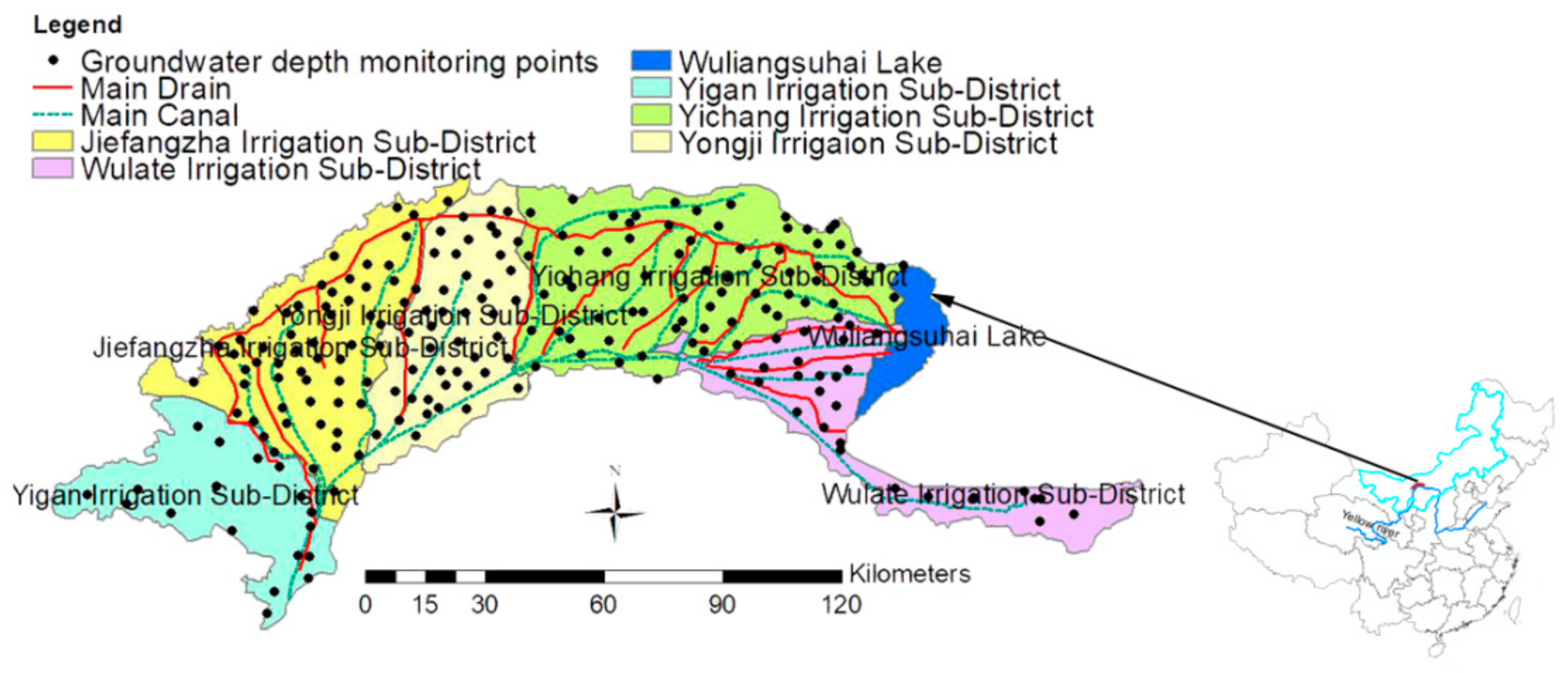
The HID is an important food production area, located in the western arid areas of the Inner Mongolia autonomous region of Northwest China (Figure 1). The study area has a typically arid and semi-arid continental climate, and the mean annual rainfall and annual pan evapotranspiration are approximately 130–210 mm and 2100–2300 mm, respectively [7,28]. The ground elevation ranges 1007–1050 m, covering a total area of 1.12 × 10⁶ ha with 5.7 × 10⁵ ha under irrigation, of which 5.25 × 10⁵ ha are cropland [2]. The irrigation water mainly comes from the Yellow River, which has an average salt concentration of approximately 0.85 dS/m. The water flows into the district through general irrigation canals that run southwest to northwest alongside the river [29]. The main soil textures in the study area are silt sand, sandy loam, and loam. The crop-growing season is from April to October, and spring wheat, spring maize, and sunflowers are the main crops in the HID.
2.2. SAHYSMOD Model Description
2.2.1. Technical Details of SAHYSMOD
SAHYSMOD is a spatial agro-hydro-salinity simulation model that can be used to predict and analyze long-term water and salt dynamics under different geohydrologic conditions, varying water management options, including the re-use of groundwater for irrigation by pumping from wells (conjunctive use), and several crop rotation schedules. The aquifer may be unconfined or semiconfined. Optionally, the responses of farmers can be simulated by adjusting agriculture and irrigation to waterlogging and salinity. The model combines the agro-hydro-salinity model SaltMod and an adjusted/extended polygonal groundwater model SGMP [30]. The SaltMod model calculates the downward and/or upward water fluxes in the soil profile for each polygon depending on the fluctuation of the groundwater table. The SGMP calculates the groundwater flows into and out of each polygon and the groundwater levels of each polygon depending on the upward and/or downward water fluxes. The above two parts interact as they influence each other. The third part is a salt balance model, which runs parallel to the water balance model and determines the salt concentrations in the soil profile, and of the drainage, well, and groundwater [27].
2.2.2. Principles of SAHYSMOD
Oosterbaan, the developer of the two models, upgraded the SALTMOD model to SAHYSMOD to enable simulation in the horizontal dimension. SALTMOD is a point-based model, with a vertical 1 D extension to address solute transport in the Z-axis but lacks the possibility of associating the horizontal relationship of points in the plane. In contrast, SAHYSMOD can be considered as a 2D model, which considers spatial variations by a nodal network of polygons [20].
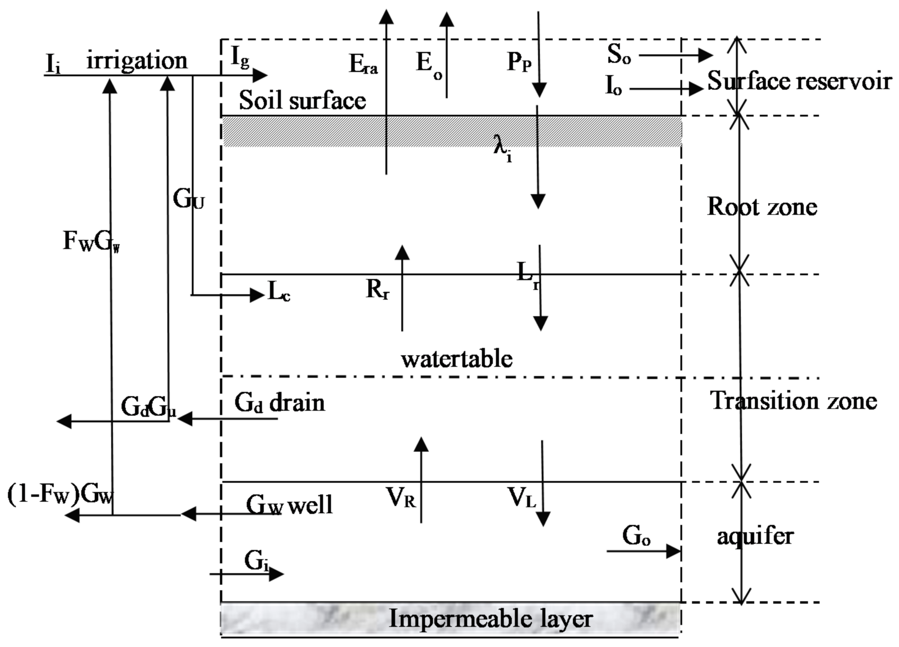
The SAHYSMOD model permits division of the study area into a maximum of 240 internal and 120 external polygons with a minimum of 3 and a maximum of 6 sides each. The spatial variations in cropping, drainage, and groundwater of the study area are defined by a nodal network of rectangular polygonal configurations, the centroid of each polygon is taken as the representative of the whole unit grid, and each grid is treated as a separate soil unit. According to the climate conditions, crop growth, irrigation, or fallow period, a year can be divided into 1–4 simulation seasons, and the length of each season can be determined according to its continuous month. In the vertical direction, the soil profile is divided into four layers: Surface reservoir, root zone, transition zone, and aquifer (Figure 2). Each layer has a water and salt balance equation, which is based on the water balance equation of each layer and its salt content. Groundwater flow is determined based on the finite difference method.
2.2.3. Data Required
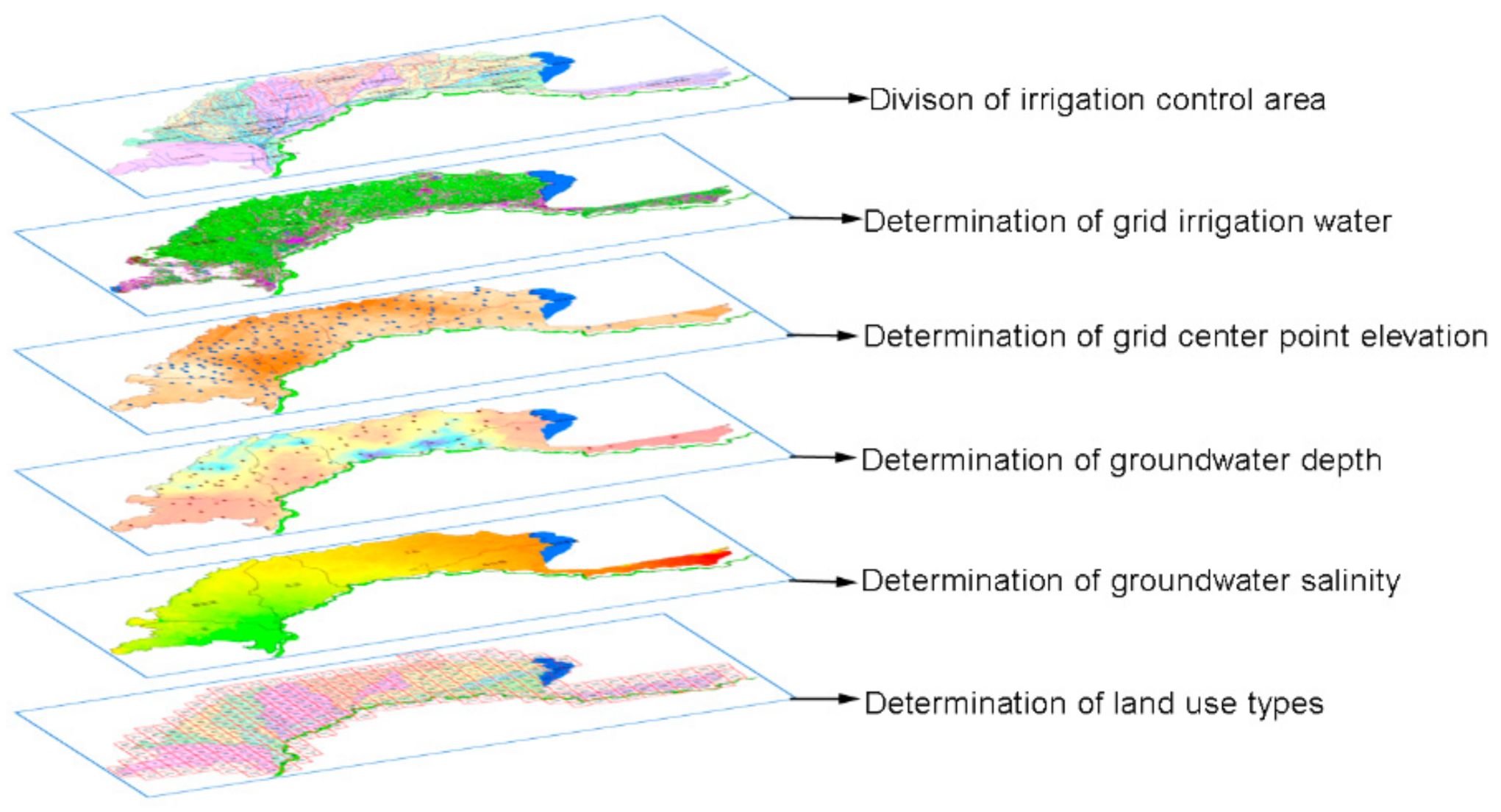
The SAHYSMOD model was primarily developed to predict long-term trends, which are based on seasonal input data and returns seasonal outputs. The input data are used to relate surface water hydrology (e.g., rainfall, potential evapotranspiration, irrigation, reuse of drainage water, and runoff) to groundwater hydrology (e.g., upward seepage, groundwater pumping, capillary rise, and drainage). The output data comprise hydrological and salinity aspects. In this study, the input data for the model included climatic data, soil properties, crop parameters, and irrigation and drainage system layouts. The required data per polygon were polygonal characteristics, hydraulic conductivity, and soil porosity. The further needed data were the leaching efficiency of the root zone, transition zone, and aquifer zone, parameters of the drainage system, and capillary rise factors. Seasonal data encompassed rainfall, irrigation, and evapotranspiration. These data were mainly collected from water and salt monitoring tests, soil sampling, and irrigation and drainage management at the Hetao Irrigation District Administration Bureau and surrounding experimental stations.
Figure 3 illustrates the input data extraction map of the grid center points in the study area. Groundwater was abstracted mainly through a number of shallow tube wells. The temporal dynamics of the groundwater table were monitored through a network of 248 observation wells distributed in the study area, and the monitoring frequency was once per 5 days. Among the 248 groundwater observation wells in the irrigation district, 91 wells synchronously monitored the groundwater salinity at a 50-day frequency. The irrigation amount per unit area was obtained by dividing the total water diversion volume of the final channel in the control area by the irrigation area of the control area, and the water diversion data of the channel were the monitoring values of the irrigation district administration. Canal water quality had an EC of 0.85 dS m−1. The surface elevation and land-use data were obtained using a DEM elevation map and interpretation of remote sensing data. ArcGIS built-in tools were used to obtain average input values of groundwater level, rainfall, and salt content in the center of each polygon.
Meteorological data from the period 2007–2016 were collected from the local meteorological station. The daily reference evapotranspiration (ET0) was calculated by the FAO Penman–Monteith method [31], and then the potential crop evapotranspiration (ETc) was determined by the crop coefficient approach [7,32]. Finally, the planting area proportion and evapotranspiration of different crops were used to calculate the seasonal potential crop evapotranspiration [15]. The soil sample collection sites for the model were based on the salt monitoring points in the study area. At each observation point, five samples were taken from five different depth intervals: 0–20, 20–40, 40–60, 60–80, and 60–90 cm.
2.2.4. Grid Generation in the Study Area
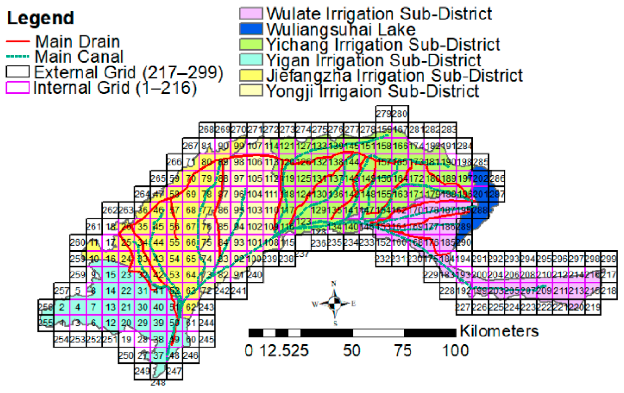
The study area was subdivided into 299 square polygons (216 internal and 83 external) via a nodal network, each 7.8 × 7.8 km in size, on a scale of 1:10,000. Each node was considered a separate unit and the centroid was taken as representative of the entire polygonal area. The external nodes are the boundary conditions that act as head-controlled boundaries for the internal nodes. The whole year was divided into three simulation seasons, namely the summer irrigation period (May to September), the autumn irrigation period (October to November), and the non-growing period (December to April). Figure 4 shows the nodal network configuration of the SAHYSMOD model, and the theoretical details of water and salt movement in SAHYSMOD are provided in [30].
3. Results and Discussion
3.1. Calibration and Validation of SAHYSMOD
Before SAHYSMOD can be used to study the long-term effects of various water management scenarios on water and salt dynamics, it needs to be calibrated and validated for a certain number of years. In this study, the model was calibrated for a six-year period, from April 2007 to April 2012, and subsequently validated using the observed salt concentration of the drainage water, groundwater depth, and drain discharge data for a four-year period, from April 2013 to April 2016. The calibrated SAHYSMOD was then used to simulate the water and salt dynamics under different water management conditions. Table 1 and Table 2 list the input parameters required by the SAHYSMOD model.
In the SAHYSMOD model input data requirements, some spatially distributed input datasets, such as the leaching efficiency of the root zone (Flr), transition zone (Flx), aquifer (Flq), and horizontal hydraulic conductivity of the aquifer (Kaq), are difficult to observe on a watershed scale. Thus, these soil hydraulic input parameters need to be determined by calibration. Kaq was determined by spatial interpolation of the measured data. Flq was determined by running trials with the model using different values of Flq and choosing the value that produced the salt concentration of the groundwater with the actual measured values. Other parameters affecting the rootzone storage efficiency and drainage rate of soil salinity could be determined by referring to relevant regional experience values or relevant literature [15], including the values of Flx and Flr.
3.1.1. Determining Kaq
In the SAHYSMOD model, the aquifer plays an important role in horizontal exchanges. In previous studies, the parameter calibration method was usually used to determine the value of Kaq. Huang et al. (2020) [33] used this method to determine a Kaq of 10 m/day in the Yinbei irrigation district of Ningxia, while the spatial variability of Kaq was not considered. One study showed that the groundwater depth is sensitive to Kaq, and that the groundwater depth increases with an increase in Kaq [26]. This was also consistent with the research conclusion of Singh and Panda (2012) [24].
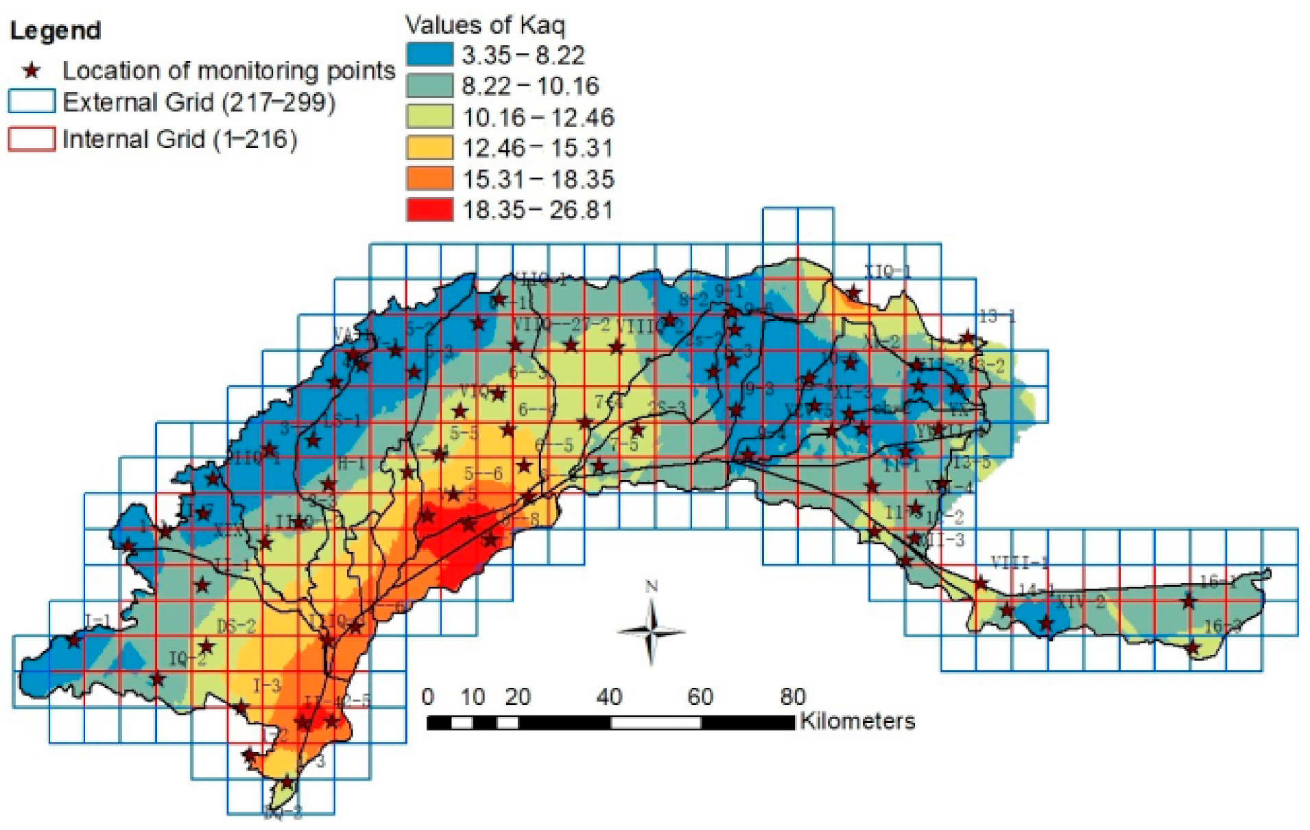
In this study, the spatial variation of aquifer properties was considered, and the spatial interpolation method was used to determine Kaq. According to the evenly distributed borehole data in the study area, the hydrogeological parameter Kaq determined by the pumping test was taken as the basic data, and the ordinary kriging method was used for spatial interpolation. Then, the Kaq value of each grid center point was extracted based on the GIS data extraction function. Figure 5 shows the Kaq spatial interpolation results in the study area. Kaq decreases from south to north in the HID and varies 3–13 m/day.
3.1.2. Determining Flq
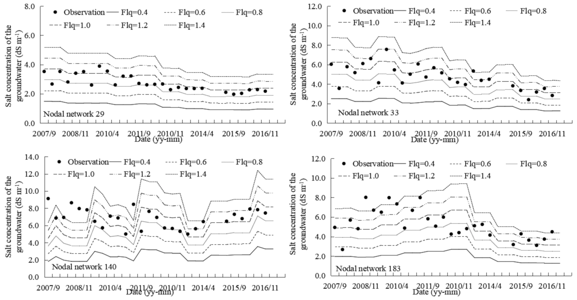
The leaching efficiency of the aquifer (Flq) is defined as the ratio of the salt concentration of the water outflowing from the aquifer to the average concentration of the water in the aquifer when saturated, and the values range from 0.01 to 2.0 in the SAHYSMOD model, firstly, simulating the groundwater salt concentration based on the arbitrary values of 0.4, 0.6, 0.8, 1.0, 1.2, and 1.4 for aquifer zones. Then, the simulated values of the groundwater salt concentration were compared with the measured values (Figure 6). Finally, the value of Flq was determined according to the best-matched measured values of Flq.
The polygonal grids 29, 33, 140, and 183 were randomly selected to calibrate Flq. The simulation results show that the measured groundwater salinity value was 0.8–1.2 of the aquifer leaching rate, which is closer to 1.0. Thus, the Flq value of 1.0 was chosen and used in all subsequent calculations. Yao et al. (2017) [26] found that the Flq of 1.2 in the aquifer corresponded well with the actually measured data in the Jiangsu rainfed farmland experimental area. Using SAHYSMOD, it was found that the higher the Flq value, the higher the groundwater salinity. However, it is obvious that the groundwater depth and drainage are insensitive to Flq [25].
3.1.3. Error Analysis
To evaluate the goodness of fit of the calculated and observed state variables, the mean relative error (MRE), relative error (RE), and the root mean square error (RMSE) were used in this study. These indicators [34,35] were defined as follows:
where N is the total number of observations, Oi is the observed value for observation i, and Pi is the calculated or simulated value for observation i(i = 1 to N).
The calibrated and validated SAHYSMOD model was applied to the following study. The polygonal grids 14 and 29 were randomly selected to compare and analyze the simulated and predicted groundwater depths of the grids, and the statistical index analysis is shown in Table 3. The RMSE of the annual variation range of the groundwater depth in the polygonal grids 14 and 29 was 0.17 and 0.29 m, respectively, and the MRE was 1.35% and 4.52%, respectively, for the calibration period. The RMSE of the annual variation range of groundwater depth was 0.22 and 0.28 m, respectively, and the MRE was 8.14% and 4.36%, respectively, for the validation period.
Overall, the simulated values of the annual average groundwater depth were close to the measured values, while the values varied significantly for different seasons, which may be due to autumn irrigation and freeze–thaw in the irrigation district. The freeze–thaw period of the HID mainly occurs from late November to May of the following year. Part of the autumn irrigation water begins to freeze in the upper soil layer in late November and does not reach the aquifer; thus, part of the groundwater in season 3 is from the freeze–thaw period of season 2 (autumn irrigation period) due to the later ablation. The model does not consider this freeze–thaw problem and, therefore, the simulated groundwater depth value in season 2 is slightly less than the measured value, and the simulated value in season 3 is higher than the measured value.
The water discharge in each season is also greatly affected by autumn irrigation and the freeze–thaw period. During the growth period, a part of the water discharge may come from the freeze–thaw of the previous year’s autumn irrigation, which would lead to the measured value of the water discharge in the growth period being greater than the simulated value. Therefore, the annual drainage was adopted in this study for comparative analysis (Table 4). The RE was between 0.30% and 9.08% for the calibration and validation period.
Grid 196 is located near the outlet of the main drainage ditch in the irrigation district and its conductivity was taken as representative for the drainage water salinity in the HID. Table 5 shows statistics comparing simulated and measured drainage water salinity. The RE was between 0.05% and 12.48% for the calibration period, and between 1.70% and 14.83% for the validation period. As the drainage water salinity is greatly affected by external interferences, there is a big difference between the simulated and measured values in some of the years simulated. However, overall, the average RE of the drainage conductivity was 7.07% for the calibration and validation periods, i.e., within the acceptable range.
Generally, the model produced a good simulation effect after calibration and validation and achieved a reliable verification for local conditions. The model could thus be applied for further studies to simulate and analyze the water and salt dynamics.
3.2. Scenario Setting
Scenario 1: Schemes for reducing total water diversion from the canal head.
Assuming that the current planting structure, the fraction of lined to the total length of the canal, and field water-saving measures remain constant, four schemes were set to reduce the total water diversion by –5%, –10%, –15%, and –20%, respectively.
Scenario 2: Schemes for improving the water efficiency of the canal system.
The water efficiency of the canal system (ŋ) reflects the utilization efficiency of water from the canal head to the field at all levels of the canals. Keeping the total water diversion and other conditions constant, η was increased by 10% and 20% (η = 0.592, and 0.646), based on the current η in each sub-irrigation district.
Scenario 3: Different water-saving combination schemes.
In this scenario, it was assumed that the planting structure and field water-saving measures remain constant, that is, the irrigation water quantity of the last canal entering the field is constant (IAA and IAB inputs). Considering the total water diversion and the water efficiency of the canal system, six different values of η were set, respectively; that is, η was increased by 5.3%, 10.0%, 17.6%, 20%, and 25% based on the existing water efficiency of canal system water-use coefficient. Accordingly, the total water diversion could be reduced by 5.0%, 9.0%, 15.0%, 16.7%, and 20%, respectively. The five different water-saving combination schemes are listed in Table 6.
3.3. Scenario Simulation
3.3.1. Current Irrigation and Drainage Management Scheme
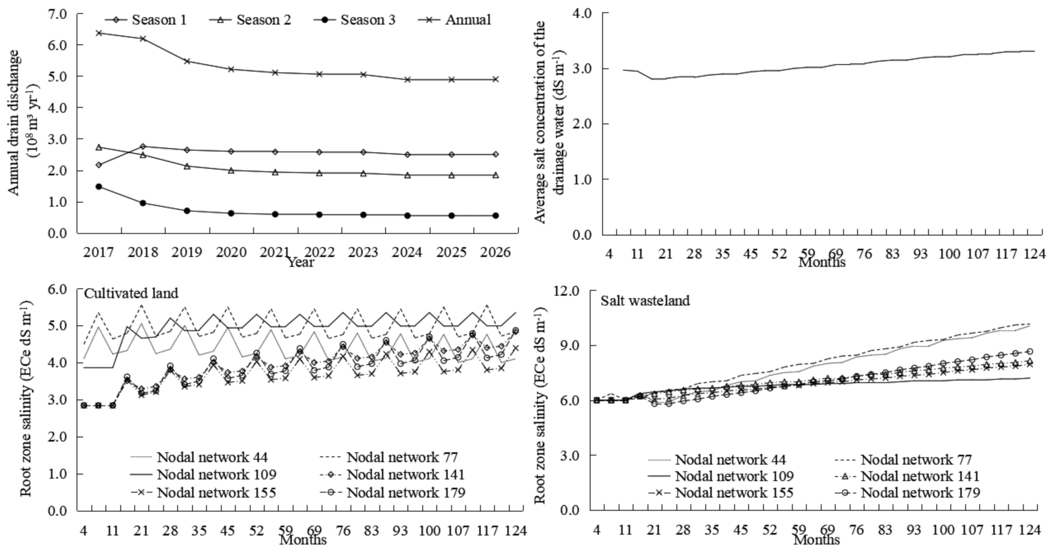
Figure 7 shows the changes in drainage quantity and drainage water salinity, and the soil salinity dynamics of the cultivated land and salt wasteland under current water management conditions based on the calibrated and validated SAHYSMOD model. As can be seen, the annual drainage volume of the total irrigation area first decreased and then gradually stabilized over the next 10 years, with average annual drainage of 531 million m3·yr–1. However, the salt concentration of the drainage water increased only slightly.
Grids 44, 77, 109, 141, 155, and 179 were selected to represent different irrigation areas. As shown in Figure. 7, the root zone salinity of grids 44, 77, and 109, which are located in the middle and upper reaches of the irrigation area, slightly decreased or remained basically stable for cultivated land. However, the root zone salinity of grids 141, 155, and 179, which are located in the lower reaches of the irrigation area, increased significantly. This is consistent with the spatial variation of soil salinity in the HID. Salinization in the lower reaches of the irrigation area is more serious due to poor drainage and shallower groundwater depths. The root zone salinity of the cultivated land significantly fluctuated seasonally, and the soil salinity value showed an obvious decreasing trend in the autumn irrigation period. The salinity of the salt wasteland showed a continuously increasing trend, which is consistent with the results of a previous study [15]. The water table of the salt wasteland is deeper than in the neighboring irrigated land, with the result that it attracts the groundwater from the irrigated area, thus the salts from the cultivated fields are removed and collected in the wasteland, which becomes very salty.
3.3.2. Schemes for Reducing Total Water Diversion from the Canal Head
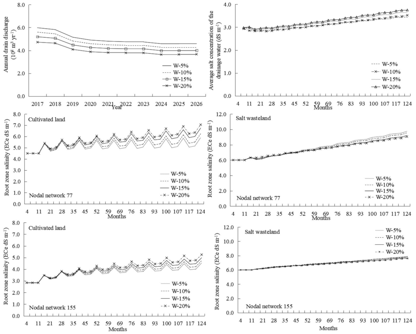
In this scenario, all other parameters remained constant and the influence of water and salt dynamics on the total water diversion from the canal head was studied. Figure 8 shows that with a decrease in the total water diversion from the canal head, the annual drainage volume decreased while the drainage water salinity visibly increased. When the total water diversion was reduced by 20%, the annual drainage volume decreased from 531 million m3·yr–1 to 397 million m3·yr–1 and the drainage water salinity increased from 3.31 dS m–1 to 3.71 dS m–1 over the next 10 years. Furthermore, the soil salinity of the cultivated land significantly fluctuated seasonally, and the salinity of the cultivated land increased with the decrease in total water diversion during the same time. This is because, under the condition that the current fraction of the lined to the total length of the canal remains constant, the leakage of the canal system and the amount of water discharged from the last channel into the field was reduced, which led to a decrease in groundwater recharge and annual drainage volume. Accordingly, the amount of autumn irrigation for salt leaching also decreased; thus, the desalination effect was not obvious. The soil salinity of the salt wasteland continuously increased and was less affected by the amount of water diverted. After the end of the simulation period, taking grid 77 as an example, the soil salinity of W1, W2, W3, and W4 increased by 31.26%, 39.04%, 50.16%, and 56.84%, respectively. The annual drainage salinity of the four schemes increased by 15.48%, 18.43%, 21.47%, and 24.49%, respectively. The annual salt discharges are 89.22 t·yr–1, 85.11 t·yr–1, 82.13 t·yr–1, and 76.13 t·yr–1, respectively. From the point of view of salt discharge in the irrigation area and soil salt control in the cultivated land, the W1 scenario is the best, but this scheme needs the largest total water diversion from the canal head.
3.3.3. Schemes for Improving the Water Efficiency of the Canal System
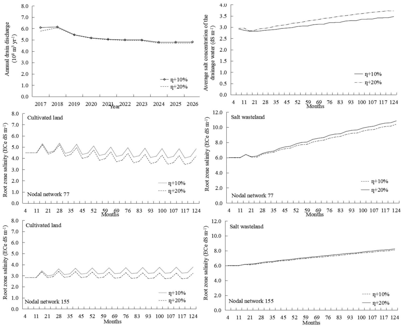
In this scenario, all other parameters were kept constant and different water efficiency of the canal system was set. When the total water diversion from the canal head was fixed, improving the water efficiency of the canal system reduced the leakage of the channel and the amount of groundwater supplied through the channel, while the irrigation water quantity of the last stage channel entering the field increased. Thus, the annual drainage and groundwater depth are affected by the leakage of the canal system and field. Figure 9 shows that the annual drainage volume first decreased and then gradually stabilized with the passage of time. In the early stage of the simulation, the drainage decreased greatly, while it gradually became stable in the later stage. This indicates that the leakage of the canal system has a great influence on the drainage volume of the irrigation area, while the influence of the drainage amount of the irrigation area from an increasing water efficiency of the canal system decreased when η was improved to a certain extent. This is mainly due to the gradual stabilization of the groundwater depth with the passage of time. The drainage water salinity increased with the improvement of η because the high η resulted in a small leakage from the irrigation canals and large irrigation water quantities entering the field. A larger autumn irrigation leaching salt will lead to a higher drainage water salinity. Simultaneously, the root zone salinity of the cultivated land significantly fluctuated seasonally and decreased with the improvement of η in the same period due to the larger autumn irrigation leaching salt. Thus, the water efficiency of the canal system has a great influence on controlling the root zone salinity of the cultivated land. After the end of the simulation period, taking grid 77 as an example, when the η = 10%, the soil salinity of cultivated land increased by 7.8%, the annual drainage water salinity increased by 11.1%, and the annual salt discharge was 95.15 t·yr–1; When η = 20%, the soil salinity of cultivated land decreased by 6.5%, the annual drainage salinity increased by 17.1%, and the annual salt discharge was 99.49 t·yr–1. From the point of view of salt discharge in the irrigation area and soil salt control in cultivated land, the scenario of η = 20% is the best.
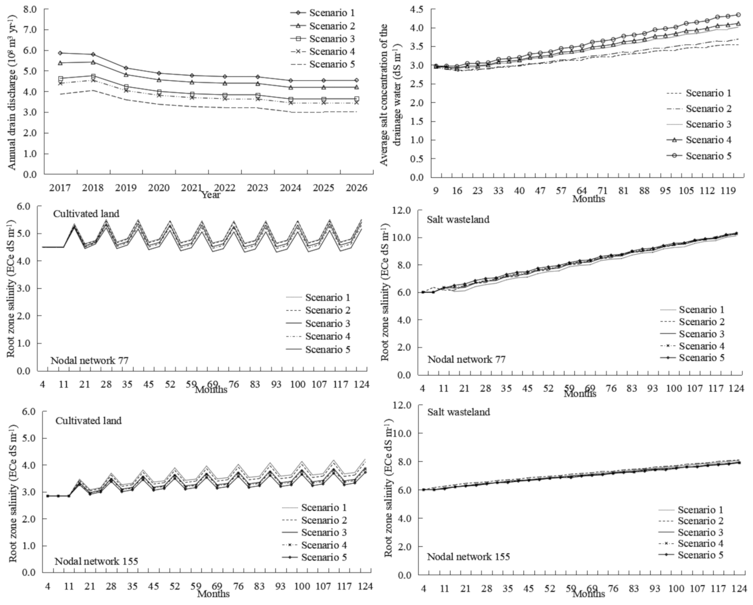
3.3.4. Different Water-Saving Schemes
As shown in the previous two sections, the leakage of water from the canal and the irrigation water quantity of the last canal entering the field will change according to the reduction of the total water diversion from the canal head and improvement of the water efficiency of the canal system. In this scenario, the irrigation water quantity of the last canal entering the field is constant, the η was improved, and the total water diversion from the canal head was decreased. Figure 10 shows the variation in the water and salt dynamics under different water-saving schemes. During the same period, the higher η was, the greater the annual drain discharge became. Scenario 6 had the highest η and the smallest annual drain discharge of 336 million m3·yr–1, while scenario 1 had the lowest η and the largest annual drain discharge of 495 million m3·yr–1. It can also be seen that the drainage water salinity increased with the increase of η at a constant field irrigation water quantity. When the irrigation quota was constant, and the field leakage was also constant, the annual drain discharge and groundwater depth were mainly affected by the leakage of the canal system. It can be seen that the difference in soil salinity was relatively small when the irrigation water quantity of the last canal entering the field was constant. Thus, the field irrigation quota played a significant role in controlling the root zone salinity.
After the simulation period, the increment and decrement of soil salinity of the cultivated land in the six schemes of F1, F2, F3, F4, F5, and F6 are +22.35%, +22.35%, +20.13%, +17.9%, +14.7%, and −5.78%, respectively. The increment and decrement of annual drainage water salinity are +18.5%, +23.8%, +33.8%, +36.8%, +44.1%, and −53.2%, respectively. The annual salt discharges in the irrigation area are 153.67 t·yr–1, 148.70 t·yr–1, 140.34 t·yr–1, 138.71 t·yr–1, 136.90 t·yr–1, and 135.45 t·yr–1. From the perspective of salt control of cultivated land in the soil layer, F6 has the best effect, while from the perspective of salt discharge in the whole irrigation area, F1 has the best effect. The main reason is that the salt salinity of the irrigation area can only be discharged with drainage. The drainage water salinity in scheme F1 is relatively small, but the total water diversion from the canal head is large. Therefore, the annual salt discharge in the irrigation area is the largest in scheme F1. The soil salinity of cultivated land is related to irrigation quantity, groundwater level, and so on. When the total water diversion from the canal head is large, the groundwater table will rise, and then the soil salinity can be accumulated easily in the upper layer of soil under a high temperature and strong evapotranspiration. Therefore, the soil salinity of the F1 scheme is higher.
3.3.5. Comparative Analysis of Different Schemes
Based on the actual situation of the irrigation district, the water diversion amount, field irrigation water quantity, canal system leakage water volume, and annual drain discharge under the current conditions were taken as the benchmark. The effects of the different schemes were compared and analyzed and, based on the results, appropriate water-saving strategies and measures are put forward. Table 7 presents the comparison of the calculation results of the different water-saving schemes. In summary, based on the current conditions, if the HID continues to save water in the future, and considering the minimum ecological water demand (562 million m3·yr–1) and ecological water supplement conditions to maintain the existing water surface area of Wuliangsuhai downstream of the HID, the water diversion amount in the future could be reduced by up to 15%, that is, the net water diversion amount of the HID needs at least 3663 million m3·yr–1, and the maximum water-saving volume could reach 650 million m3·yr–1.
When the total amount of water diversion is decreased by less than 5% (low level), 5–10% (medium level), and 10–15% (high level) based on the current situation, the minimum net water volume required in the HID is 4.094, 3.879–4.094, and 3.663–3.879 billion m3·yr–1, respectively. The total water diversion from the head that can be saved is 215, 215–431, and 431–646 million m3·yr–1, respectively. The annual drain discharge would be 494–499, 460–499, and 401–467 million m3·yr–1, and the ecological water supplement amount of Wuliangsuhai would be 93–98, 93–132, and 126–191 million m3·yr–1, respectively. If the field irrigation amount is kept unchanged, η needs to increase by 5.3% (0.566), 5.3–10% (0.566–0.592), and 10.0–17.6% (0.592–0.632), respectively. When the reduction of the total water diversion is not large, the improvement of field water-saving technology or the adjustment of the crop planting structure can be given priority to reduce field irrigation water. When the total water diversion is greatly reduced, the field water-saving and canal lining engineering measures must be considered comprehensively.
4. Conclusions
This paper proposes a method combining the SAHYSMOD model and GIS to predict the water and salt dynamics in large regions under different water-saving schemes. The model produced good simulation outputs after calibration (6 years) and validation (4 years) and comprehensively considers regional spatial variability and simulates regional water and salt dynamic changes under different irrigation and drainage management conditions. Comparing and analyzing the effects of different water-saving scenarios, the following conclusions were drawn.
Under existing irrigation and drainage conditions, the annual drain discharge will first decrease and then gradually stabilize over the next 10 years, with average annual drainage of 531 million m3·yr–1. However, the drainage water salinity will slightly increase. The soil salinity in the middle and upper reaches of the irrigation district decreased slightly in the simulation, while that in the lower reaches of the irrigation district increased significantly.
In the future, if the total water diversion from the canal head in the HID continues to decrease, considering the minimum ecological water demand (562 million m3·yr–1) and ecological water supplement conditions to maintain the existing water surface area of Wuliangsuhai downstream of the HID, the water diversion amount in the future could be reduced by up to 15%, that is, the net water diversion amount of the HID needs at least 3663 million m3·yr–1, and the maximum water-saving volume could reach 650 million m3·yr–1. If the field irrigation amount remains unchanged, η can be increased by 17.6% (0.632).
The influence of canal system leakage on the annual drain discharge is greater than that of field leakage. For the fixed reduction rate of total water diversion, when the soil salinity in the root zone of cultivated land meets the demand, in order to maximize the amount of drainage water and drained salt of the whole irrigation area, the prioritized measure should be given to reduce the amount of field irrigation quota, and then to improve the water efficiency of the canal system.
Based on a comparative analysis of the different water-saving schemes, we conclude that the amount of salt introduced, discharged, and accumulated in the irrigation district decreases with a decrease in total water diversion, but the salt concentration of the drainage water will increase, which will have an impact on the salinity of the Wuliangsuhai water body. Although a certain amount of water can be saved through various measures, the minimum ecological water demand required to maintain the existing water surface area and salinity in Wuliangsuhai Lake downstream of the HID should be considered comprehensively, and the optimal water management scheme should be determined based on the analysis of the actual ecological water supplement conditions in the HID.
Author Contributions
Conceptualization, X.C. and S.W.; methodology, X.C. and H.C.; investigation, X.C. and X.G.; formal analysis, X.G.; writing—original draft preparation, X.C.; writing—review and editing, Z.G. and S.W. All authors have read and agreed to the published version of the manuscript.
Funding
This work was funded by the National Key Research and Development Program of China (2019YFC0409203), China Postdoctoral Science Foundation funded project (Grant No. 2020M670386), Major Project in Key Research and Development Program of the Ningxia Hui Autonomous Region (Grant No. 2018BBF02022), Basic research program of Qinghai Province (Grant No. 2021-ZJ-709).
Institutional Review Board Statement
Not applicable.
Informed Consent Statement
Not applicable.
Data Availability Statement
The data presented in this study are available on request from the corresponding author. The data are not publicly available due to research continuation.
Conflicts of Interest
The authors declare no conflict of interest.
References
- Mirlas, V. Assessing soil salinity hazard in cultivated areas using MODFLOW model and GIS tools: A case study from the Jezre’el Valley, Israel. Agric. Water Manag. 2012, 109, 144–154. [Google Scholar] [CrossRef]
- Xu, X.; Huang, G.H.; Qu, Z.Y.; Pereira, L. Assessing the groundwater dynamics and impacts of water saving in the Hetao Irrigation District, Yellow River basin. Agric. Water Manag. 2010, 98, 301–313. [Google Scholar] [CrossRef]
- Yang, Y.T.; Shang, S.H.; Jiang, L. Remote sensing temporal and spatial patterns of evapotranspiration and the responses to water management in a large irrigation district of North China. Agric. For. Meteorol. 2012, 164, 112–122. [Google Scholar] [CrossRef]
- Yue, W.F.; Li, X.Z.; Wang, T.J.; Chen, X.H. Impacts of water saving on groundwater balance in a large-scale arid irrigation district, Northwest China. Irrig. Sci. 2016, 34, 297–312. [Google Scholar] [CrossRef]
- Chen, L.J.; Feng, Q.; Li, F.R.; Li, C.S. Simulation of soil water and salt transfer under mulched furrow irrigation with saline water. Geoderma 2015, 241–242, 87–96. [Google Scholar] [CrossRef]
- Pereira, L.S.; Goncalves, J.M.; Dong, B.; Mao, Z.; Fang, S.X. Assessing basin irrigation and scheduling strategies for saving irrigation water and controlling salinity in the upper Yellow River Basin, China. Agric. Water Manag. 2007, 93, 109–122. [Google Scholar] [CrossRef]
- Miao, Q.F.; Shi, H.B.; Goncalves, J.M.; Pereira, L. Field assessment of basin irrigation performance and water saving in Hetao, Yellow River basin: Issues to support irrigation systems modernisation. Biosyst. Eng. 2015, 136, 102–116. [Google Scholar] [CrossRef] [Green Version]
- Lekakis, E.H.; Antonopoulos, V.Z. Modeling the effects of different irrigation water salinity on soil water movement, uptake and multicomponent solute transport. J. Hydrol. 2015, 530, 431–446. [Google Scholar] [CrossRef]
- Chen, L.J.; Feng, Q.; Li, F.R.; Li, C.S. A bidirectional model for simulating soil water flow and salt transport under mulched drip irrigation with saline water. Agric. Water Manag. 2014, 146, 24–33. [Google Scholar] [CrossRef]
- Qi, Z.J.; Feng, H.; Zhao, Y.; Zhang, T.B.; Yang, A.Z.; Zhang, Z.X. Spatial distribution and simulation of soil moisture and salinity under mulched drip irrigation combined with tillage in an arid saline irrigation district, northwest China. Agric. Water Manag. 2018, 201, 219–231. [Google Scholar] [CrossRef]
- Jiang, J.; Feng, S.Y.; Huo, Z.L.; Zhao, Z.C.; Jia, B. Application of the SWAP model to simulate water–salt transport under deficit irrigation with saline water. Math. Comput. Model 2011, 54, 902–911. [Google Scholar] [CrossRef]
- Yao, R.J.; Yang, J.S.; Zhang, T.J.; Hong, L.Z.; Wang, M.W.; Yu, S.P.; Wang, X.P. Studies on soil water and salt balances and scenarios simulation using SaltMod in a coastal reclaimed farming area of eastern China. Agric. Water Manag. 2014, 131, 115–123. [Google Scholar] [CrossRef]
- Singh and Ajay. Evaluating the effect of different management policies on the long-term sustainability of irrigated agriculture. Land Use Policy 2016, 54, 499–507. [Google Scholar] [CrossRef]
- Mao, W.; Yang, J.S.; Zhu, Y.; Ye, M.; Wu, J.W. Loosely coupled SaltMod for simulating groundwater and salt dynamics under well-canal conjunctive irrigation in semi-arid areas. Agric. Water Manag. 2017, 192, 209–220. [Google Scholar] [CrossRef]
- Chang, X.M.; Gao, Z.Y.; Wang, S.L.; Chen, H.R. Modelling long-term soil salinity dynamics using SaltMod in Hetao Irrigation District, China. Comput. Electron. Agric. 2019, 156, 447–458. [Google Scholar] [CrossRef]
- Fujimaki, H.; Abd, H.M.; Mahdavi, S.M.; Ebrahimian, H. Optimization of Irrigation and Leaching Depths Considering the Cost of Water Using WASH_1D/2D Models. Water 2020, 12, 2549. [Google Scholar] [CrossRef]
- Surendran, U.; Sushanth, C.M.; Mammen, G.; Joseph, E.J. Modelling the Crop Water Requirement Using FAO-CROPWAT and Assessment of Water Resources for Sustainable Water Resource Management: A Case Study in Palakkad District of Humid Tropical Kerala, India. Aquat. Procedia 2015, 4, 1211–1219. [Google Scholar] [CrossRef]
- Xu, X.; Huang, G.H.; Qu, Z.Y.; Pereira, L.S. Using MODFLOW and GIS to Assess Changes in Groundwater Dynamics in Response to Water Saving Measures in Irrigation Districts of the Upper Yellow River Basin. Water Resour. Manag. 2011, 25, 2035–2059. [Google Scholar] [CrossRef]
- Xu, X.; Huang, G.H.; Zhan, H.B.; Qu, Z.Y.; Huang, Q.Z. Integration of SWAP and MODFLOW-2000 for modeling groundwater dynamics in shallow water table areas. J. Hydrol. 2012, 412, 170–181. [Google Scholar] [CrossRef]
- Oosterbaan, R.J. SAHYSMOD (Version 1.7a), Description of Principles, User Manual and Case Studies; International Institute for Land Reclamation and Improvement (ILRI): Wageningen, The Netherlands, 2005. [Google Scholar]
- Akram, S.; Kashkouli, H.A.; Pazira, E. Sensitive variables controlling salinity and water table in a bio-drainage system. Irrig. Drain. Sys. 2008, 22, 271–285. [Google Scholar] [CrossRef]
- Desta, T.F. Spatial Modelling and Timely Prediction of Salinization using SAHYSMOD 972 in GIS Environment (a Case Study of Nakhon Ratchasima, Thailand). Master’s Thesis, International Institute for Geo-information Science and Earth Observation, Enschede, The Netherlands, 2009. [Google Scholar]
- Singh, A.; Panda, S.N. Integrated Salt and Water Balance Modeling for the Management of Waterlogging and Salinization. I: Validation of SAHYSMOD. J. Irrig. Drain. Eng. 2012, 138, 955–963. [Google Scholar] [CrossRef]
- Singh, A.; Panda, S.N. Integrated Salt and Water Balance Modeling for the Management of Waterlogging and Salinization. II: Application of SAHYSMOD. J. Irrig. Drain. Eng. 2012, 138, 964–971. [Google Scholar] [CrossRef]
- Yao, R.J.; Wang, X.J.; Wu, D.H.; Xie, W.P. Calibration and Sensitivity Analysis of Sahysmod for Modeling Field Soil and Groundwater Salinity Dynamics in Coastal Rainfed Farmland. Irrig. Drain. 2017, 66, 411–427. [Google Scholar] [CrossRef]
- Yao, R.L.; Wang, X.J.; Wu, D.H.; Xie, W.P.; Wang, X.P.; Zhang, X. Scenario simulation of field soil water and salt balances using SahysMod for salinity management in a coastal rainfed farmland. Irrig. Drain. 2017, 66, 872–883. [Google Scholar] [CrossRef]
- Inam, A.; Adamowski, J.; Prasher, S.; Halbe, J.; Malard, J.; Albano, R. Coupling of a distributed stakeholder-built system dynamics socio-economic model with SAHYSMOD for sustainable soil salinity management-Part 1: Model development. J. Hydrol. 2017, 551, 278–299. [Google Scholar] [CrossRef]
- Xue, J.; Ren, L. Assessing water productivity in the Hetao Irrigation District in Inner Mongolia by an agro-hydrological model. Irrig. Sci. 2017, 35, 357–382. [Google Scholar] [CrossRef]
- Luo, Y.; Sophocleous, M. Two-way coupling of unsaturated-saturated flow by integrating the SWAT and MODFLOW models with application in an irrigation district in arid region of West China. J. Arid. Land. 2011, 3, 164–173. [Google Scholar] [CrossRef] [Green Version]
- Oosterbaan, R.J. SAHYSMOD, Description of Principles, User Manual and Case Studies; International Institute for Land Reclamation and Improvement: Wageningen, The Netherlands, 1995. [Google Scholar]
- Allen, R.G.; Pereira, L.S.; Raes, D.; Smith, M. Crop Evapotranspiration Guidelines for Computing Crop Water Requirements. FAO Irrigation Drainage Paper 56. 1998. Available online: http://www.avwatermaster.org/filingdocs/195/70653/172618e_5xAGWAx8.pdf. (accessed on 9 July 2021).
- Dai, J.X.; Shi, H.B.; Tian, D.L.; Xai, Y.H.; Hua, L.M. Determined of crops coeffi-cients of mian grain and oil crops in Inner Mongolia Hetao irrigated Area. J. Irrig. Drian. 2011, 30, 23–27. (In Chinese) [Google Scholar]
- Huang, Y.J.; Li, Z.; Zhuo, Z.Q.; Xing, A.; Huang, Y.F. Soil water and salt dynamics under different irrigation and drainage management scenarios based on SahysMod model. Trans. Chin. Soc. Agric. Eng. 2020, 36, 129–140. (In Chinese) [Google Scholar]
- Xu, X.; Huang, G.H.; Sun, C.; Pereira, L.S.; Ramos, T.B.; Huang, Q.Z.; Hao, Y.Y. Assessing the effects of water table depth on water use, soil salinity and wheat yield: Searching for a target depth for irrigated areas in the upper Yellow River basin. Agric. Water Manag. 2013, 125, 46–60. [Google Scholar] [CrossRef]
- Ren, D.Y.; Xu, X.; Hao, Y.Y.; Huang, G.H. Modeling and assessing field irrigation water use in a canal system of Hetao, upper Yellow River basin: Application to maize, sunflower and watermelon. J. Hydrol. 2016, 532, 122–139. [Google Scholar] [CrossRef]
Figure 1.
Location of the study area.

Figure 2.
Soil reservoirs with hydrological inflow and outflow components. Note: Pp is the amount of water vertically reaching the soil surface, such as precipitation and sprinkler irrigation; Ii is the irrigation water supplied by the canal system; Ig is the gross irrigation inflow including the natural surface inflow and the drain and well water used for irrigation, but excluding the percolation losses from the canal system; I0 is the amount of irrigation water leaving the area through the canal system (bypass); Eo is the amount of evaporation from open water; Era is the amount of actual evapotranspiration from the root zone; λi is the amount of water infiltrated through the soil surface into the root zone; λ0 is the amount of water ex-filtrated through the soil surface from the root zone; the term λ0 is not shown in Figure 2 as it can occur only when the water table is above the soil surface; So is the amount of surface runoff or surface drainage leaving the area; Lc is the percolation loss from the irrigation canal system; Lr is the amount of percolation losses from the root zone; VR is the amount of vertical upward seepage from the aquifer into the transition zone; VL is the amount of vertical downward drainage from the saturated transition zone to the aquifer; Rr is the amount of capillary rise into the root zone; Gw is the amount ground water pumped from the aquifer through wells; Gd is the total amount of subsurface drainage water; Gi and Go are the horizontally incoming/outgoing ground water flow into a polygon through the aquifer; Fw is the fraction of the pumped well water Gw used for irrigation and Gu is the quantity of subsurface drainage water used for irrigation. FwGw and Gu were negligible and were set equal to zero in this study. ΔWs is the change in the amount of water stored in the surface reservoir.

Figure 3.
Input data extraction map of grid center points in the study area.

Figure 4.
Nodal network polygonal configuration of the SAHYSMOD model.

Figure 5.
Spatial interpolation results of the horizontal hydraulic conductivity of the aquifer (Kaq).
Figure 5.
Spatial interpolation results of the horizontal hydraulic conductivity of the aquifer (Kaq).

Figure 6.
Calibration of the leaching efficiency in the aquifer zone (Flq) for SAHYSMOD.

Figure 7.
Changes in drainage quantity, drainage water salinity, soil salinity dynamics of cultivated land, and salt wasteland under the existing irrigation and drainage mode.
Figure 7.
Changes in drainage quantity, drainage water salinity, soil salinity dynamics of cultivated land, and salt wasteland under the existing irrigation and drainage mode.

Figure 8.
Variation of the annual drain discharge, drainage water salinity, and soil salinity dynamics of the cultivated land and salt wasteland under different water diversion quantities.
Figure 8.
Variation of the annual drain discharge, drainage water salinity, and soil salinity dynamics of the cultivated land and salt wasteland under different water diversion quantities.

Figure 9.
Variation of the annual drain discharge, drainage water salinity, and soil salinity dynamics of cultivated land and salt wasteland under different water efficiency of the canal system.
Figure 9.
Variation of the annual drain discharge, drainage water salinity, and soil salinity dynamics of cultivated land and salt wasteland under different water efficiency of the canal system.

Figure 10.
Variation of the annual drain discharge, drainage water salinity, and soil salinity dynamics of cultivated land and salt wasteland under different water-saving schemes.
Figure 10.
Variation of the annual drain discharge, drainage water salinity, and soil salinity dynamics of cultivated land and salt wasteland under different water-saving schemes.


Table 1.
Seasonal input data of SAHYSMOD model.
| Seasonal Data | Value | Data Sources |
|---|---|---|
| 1. Duration of seasons (months) | ||
| Season 1 (May–September) | 5 | M |
| Season 2 (October–November) | 2 | M |
| Season 3 (December–April) | 5 | M |
| 2.Water balance components | ||
| Irrigated area fraction in season 1/season 2/season 3 | 0.57/0.57/0 | R |
| Rainfall in season 1/season 2/season 3 (m) | 0.119/0.010/0.011 | M |
| Irrigation in season 1/season 2/season 3 (m) | 0.011–0.506/0.014–0.262/0 | M |
| Seasonal potential evapotranspiration (m) | 0.652–0.694/0.103–0.109/0.062–0.110 | M |
| Salinity of irrigation water season 1/season 2/season 3 (dS m–1) | 1.02 | M |
| Seasonal runoff (m) | 0 | M |
| Rootzone storage efficiency for rainfall and irrigation | 0.8 | M/G |
| Pumped well water from aquifer (m) | 0 | M |
Note: Where the rainfall and potential evapotranspiration in different seasons are calculated by daily data, they change day by day; the irrigation salinity is assumed to be uniform across the region.
Table 2.
Summary of input parameters required by SAHYSMOD.
| Polygonal Data | Value | Data Sources |
|---|---|---|
| 1.Overall system parameters | ||
| bottom level of the aquifer | 0 | M |
| Thickness of the surface reservoir (m) | 0 | M |
| Thickness of the root zone (m) | 1 | M |
| Thickness of the transition zone (m) | 4 | M |
| Thickness of the aquifer zone (m) | 90 | M |
| Index for phreatic or semi-confined aquifer (0 = phreatic,1 = semi-confined) | 0 | M |
| 2.Soil and aquifer properties | ||
| Total porosity of the root zone (Ptr) | 0.48 | G |
| Total porosity of the transition zone (Ptx) | 0.48 | G |
| Total porosity of the aquifer zone (Ptq) | 0.4 | G |
| Effective porosity of the root zone (Per) | 0.07 | G |
| Effective porosity of the transition zone (Pex) | 0.07 | G |
| Effective porosity of the aquifer zone (Peq) | 0.1 | G |
| Leaching efficiency of the root zone (Flr) | 0.85 | G/C |
| Leaching efficiency of the transition zone (Flx) | 0.65 | G/C |
| Leaching efficiency of the aquifer zone (Flq) | 0.9 | G/C |
| Horizontal hydraulic conductivity of the aquifer zone (m/day) | 6.08–13.66 | M |
| 3.Initial and boundary conditions | ||
| Initial salt concentration of soil moisture in the root zone (dS m–1) | 5.47-6.99 | M |
| Initial salt concentration of soil moisture in the transition zone (dS m–1) | 4.14–5.70 | M |
| Initial salt concentration of soil moisture in the aquifer zone (dS m–1) | 3.86–6.75 | M/K |
| Initial groundwater level with respect to reference level (Hw) (m) | 1005–1211 | M/K |
| Constant inflow condition into the aquifer (m yr–1) | 0 | M/G |
| Constant outflow condition into the aquifer (m yr–1) | 0.1 | M/G |
| Critical depth of the groundwater table for capillary rise (m) | 2.3–2.5 | M |
| Drain depth (m) | 1.5 | M |
| Drain spacing (m) | 100 | M |
Note: Where M represents the parameters obtained by the actual measurement or calculation of investigation data, C represents the parameters obtained by the model calibration, R represents the parameters obtained by remote sensing interpretation, K represents the parameters obtained through spatial interpolation, and G is defined by the related references.
Table 3.
Comparison of measured and simulated groundwater depth.
| Polygonal Number | Date | Groundwater Depth | ||||
|---|---|---|---|---|---|---|
| Observation (m) | Simulation (m) | RMSE (m) | MRE (%) | |||
| Nodal network 14 | Calibration period (2007–2012) | Season 1 | 1.90 | 1.63 | 0.39 | 14.54 |
| Season 2 | 1.15 | 0.94 | 0.55 | 18.54 | ||
| Season 3 | 1.72 | 2.17 | 0.71 | −26.30 | ||
| Annual average | 1.59 | 1.61 | 0.17 | −1.35 | ||
| Validation period (2013–2016) | Season 1 | 1.77 | 1.70 | 0.11 | 3.94 | |
| Season 2 | 1.29 | 1.20 | 0.36 | 7.64 | ||
| Season 3 | 1.61 | 2.16 | 0.72 | −34.04 | ||
| Annual average | 1.56 | 1.69 | 0.22 | −8.14 | ||
| Nodal network 29 | Calibration period (2007–2012) | Season 1 | 2.00 | 1.54 | 1.21 | 23.30 |
| Season 2 | 0.96 | 0.93 | 0.27 | 2.58 | ||
| Season 3 | 1.75 | 2.03 | 0.77 | −15.88 | ||
| Annual average | 1.57 | 1.50 | 0.29 | 4.52 | ||
| Validation period (2013–2016) | Season 1 | 2.10 | 1.62 | 1.00 | 22.83 | |
| Season 2 | 1.17 | 1.13 | 0.45 | 4.22 | ||
| Season 3 | 1.72 | 2.03 | 0.86 | −18.08 | ||
| Annual average | 1.67 | 1.59 | 0.28 | 4.36 | ||
Table 4.
Comparison of measured and simulated annual discharge.
| Date | Observation (108 m3 yr–1) | Simulation (108 m3 yr–1) | RE (%) | |
|---|---|---|---|---|
| Calibration period | 2007 | 5.17 | 5.63 | 9.08 |
| 2008 | 6.28 | 6.12 | 2.52 | |
| 2009 | 4.97 | 5.34 | 7.53 | |
| 2010 | 5.52 | 5.68 | 3.02 | |
| 2011 | 5.00 | 4.82 | 3.53 | |
| 2012 | 7.30 | 7.28 | 0.24 | |
| Validation period | 2013 | 5.96 | 6.05 | 1.56 |
| 2014 | 7.45 | 7.47 | 0.30 | |
| 2015 | 6.13 | 6.17 | 0.70 | |
| 2016 | 6.25 | 6.20 | 0.76 | |
Table 5.
Statistics comparing simulated and measured drainage water salinity.
| Date | Observation (dS m–1) | Simulation (dS m–1) | RE (%) | |
|---|---|---|---|---|
| Calibration period | 2007 | 4.45 | 4.36 | 2.11 |
| 2008 | 4.47 | 3.91 | 12.48 | |
| 2009 | 4.47 | 4.47 | 0.05 | |
| 2010 | 4.34 | 3.94 | 9.22 | |
| 2011 | 3.94 | 4.08 | 3.54 | |
| 2012 | 3.92 | 3.71 | 5.40 | |
| Validation period | 2013 | 3.86 | 3.79 | 1.70 |
| 2014 | 2.67 | 3.03 | 13.37 | |
| 2015 | 3.28 | 3.46 | 5.62 | |
| 2016 | 2.55 | 2.93 | 14.83 | |
Table 6.
Combination of different water-saving schemes.
| Scenario | Water Efficiency of the Canal System (η) | Total Water Diversion from the Canal Head (W) |
|---|---|---|
| Scenario 1 | 0.566 (+ 5.3%) | −5.0% |
| Scenario 2 | 0.592 (+ 10.0%) | −9.0% |
| Scenario 3 | 0.632 (+ 17.6%) | −15.0% |
| Scenario 4 | 0.646 (+ 20.0%) | −16.7% |
| Scenario 5 | 0.673 (+ 25.0%) | −20.0% |
Table 7.
Comparison of calculation results of different water-saving schemes.
| Scenarios | Total Water Diversion from the Canal Head (108 m3·yr–1) | Leakages from Irrigation Canal (108 m3·yr–1) | Irrigation Quantity (108 m3·yr–1) | Drain Discharge (108 m3·yr–1) | Salt Concentration of the Drainage Water (ds·m–1) | Water Replenishment Required by Wuliangsuhai (108 m3·yr–1) | Amount of Salt Introduced (104 t·yr–1) | Amount of Salt Discharge (104 t·yr–1) | Amount of Salt Accumulated (104 t·yr–1) | |
|---|---|---|---|---|---|---|---|---|---|---|
| Current conditions | 43.10 | 19.91 | 23.19 | 5.31 | 3.31 | 0.61 | 258.59 | 94.88 | 163.71 | |
| Schemes for reducing total water diversion from the canal head | W–5% | 40.94 | 18.92 | 22.03 | 4.99 | 3.42 | 0.93 | 245.66 | 89.22 | 156.44 |
| W–10% | 38.79 | 17.92 | 20.87 | 4.67 | 3.42 | 1.26 | 232.73 | 85.11 | 147.62 | |
| W–15% | 36.63 | 16.92 | 19.71 | 4.34 | 3.61 | 1.58 | 219.80 | 82.13 | 137.67 | |
| W–20% | 34.48 | 15.93 | 18.55 | 3.97 | 3.70 | 1.96 | 206.87 | 76.37 | 130.50 | |
| Schemes for improving the water efficiency of the canal system | η + 10% | 43.10 | 17.59 | 25.51 | 5.23 | 3.42 | 0.70 | 258.59 | 95.15 | 163.44 |
| η + 20% | 43.10 | 15.27 | 27.82 | 5.15 | 3.70 | 0.77 | 258.59 | 99.49 | 159.10 | |
| Different water-saving combination schemes | Scenario 1 | 40.94 | 17.75 | 23.19 | 4.94 | 3.51 | 0.98 | 245.66 | 91.99 | 153.67 |
| Scenario 2 | 39.22 | 16.01 | 23.21 | 4.60 | 3.63 | 1.32 | 235.32 | 86.62 | 148.70 | |
| Scenario 3 | 36.63 | 13.46 | 23.18 | 4.01 | 3.93 | 1.91 | 219.80 | 79.46 | 140.34 | |
| Scenario 4 | 35.90 | 12.72 | 23.18 | 3.81 | 4.03 | 2.11 | 215.40 | 76.70 | 138.71 | |
| Scenario 5 | 34.48 | 11.29 | 23.19 | 3.36 | 4.25 | 2.56 | 206.87 | 69.97 | 136.90 | |
Publisher’s Note: MDPI stays neutral with regard to jurisdictional claims in published maps and institutional affiliations. |
© 2021 by the authors. Licensee MDPI, Basel, Switzerland. This article is an open access article distributed under the terms and conditions of the Creative Commons Attribution (CC BY) license (https://creativecommons.org/licenses/by/4.0/).
Share and Cite
MDPI and ACS Style
Chang, X.; Wang, S.; Gao, Z.; Chen, H.; Guan, X. Simulation of Water and Salt Dynamics under Different Water-Saving Degrees Using the SAHYSMOD Model. Water 2021, 13, 1939. https://doi.org/10.3390/w13141939
AMA Style
Chang X, Wang S, Gao Z, Chen H, Guan X. Simulation of Water and Salt Dynamics under Different Water-Saving Degrees Using the SAHYSMOD Model. Water. 2021; 13(14):1939. https://doi.org/10.3390/w13141939
Chicago/Turabian StyleChang, Xiaomin, Shaoli Wang, Zhanyi Gao, Haorui Chen, and Xiaoyan Guan. 2021. "Simulation of Water and Salt Dynamics under Different Water-Saving Degrees Using the SAHYSMOD Model" Water 13, no. 14: 1939. https://doi.org/10.3390/w13141939
Note that from the first issue of 2016, this journal uses article numbers instead of page numbers. See further details here.