
Avocado cv. Hass Needs Water Irrigation in Tropical Precipitation Regime: Evidence from Colombia


1
Escuela EIDENAR, Facultad de Ingeniería, Universidad del Valle, Calle 13 No. 100-00, Cali 760032, Colombia
2
Facultad de Ciencias Agropecuarias, Universidad Nacional de Colombia, Sede Palmira 763533, Valle del Cauca, Colombia
3
Departamento de Agronomía, Facultad de Ciencias Agrarias, Universidad Nacional de Colombia, Sede Bogotá 111321, Colombia
*
Author to whom correspondence should be addressed.
Water 2021, 13(14), 1942; https://doi.org/10.3390/w13141942
Submission received: 26 May 2021
/
Revised: 9 July 2021
/
Accepted: 11 July 2021
/
Published: 14 July 2021
(This article belongs to the Special Issue Feature Papers of Water, Agriculture and Aquaculture)
Abstract
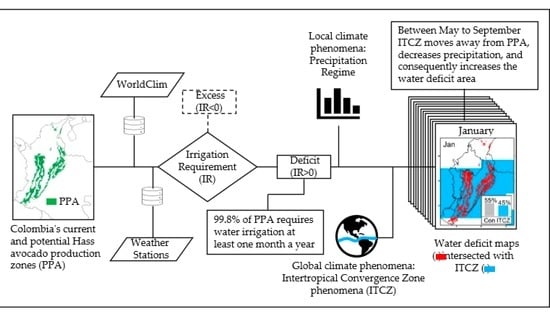
:The primary natural source of water for the Hass avocado crop in the tropics is precipitation. However, this is insufficient to provide most crops’ water requirements due to the spatial and temporal variability. This study aims to demonstrate that Hass avocado requires irrigation in Colombia, and this is done by analyzing the dynamics of local precipitation regimes and the influence of Intertropical Convergence Zone phenomena (ITCZ) on the irrigation requirement (IR). This study was carried out in Colombia’s current and potential Hass avocado production zones (PPA) by computing and mapping the monthly IR, and classifying months found to be in deficit and excess. The influence of ITCZ on IR by performing a metric relevance analysis on weights of optimized Artificial Neural Networks was computed. The water deficit map illustrates a 99.8% of PPA requires water irrigation at least one month a year. The movement of ITCZ toward latitudes far to those where PPA is located between May to September decreases precipitation and consequently increases the IR area of Hass avocado. Water deficit visualization maps could become a novel and powerful tool for Colombian farmers when scheduling irrigation in those months and periods identified in these maps.
1. Introduction
Avocado fruit production (Persea americana Mill), especially the cv. Hass, represents an important agribusiness in many countries, such as Mexico, Indonesia, the United States of America, Dominican Republic, Colombia, Chile, Peru, among others [1]. In countries such as Colombia, the planted area with Hass avocado has significantly increased in recent years [2]. Still, the industry has presented some technological limitations in selecting regions with appropriate soil and climatic conditions for planting this species [3]. Recently in Colombia, climate variability has generated drought conditions that negatively affect yields in avocado production systems with a high impact on water availability [4,5,6].
Water is critical to Hass avocado production. Water takes part in physiological processes that determine the period and intensity of growth flushes [7]. A deficit of water in trees shrinks the trunk diameter and decreases stomatal conductance, stem water potential, net photosynthesis, and net CO2 assimilation [8]. Moreover, water is directly linked with yield and fruit quality. Water deficit in this crop decreases the potential productivity [9], and leads to fruit disorders [10,11]. In fruit preharvest stages, water deficit forces the avocado tree to redistribute the water, increasing the fruit dry matter, delaying the ripening process [12], and reducing the overall quality of the fruit [11,13].
The primary natural source of water for the crop is precipitation. In tropical countries where the cultivar Hass is grown, the amount and distribution of rainfall are controlled not only by local but also by global phenomena [14,15]. Local phenomena are influenced by the relief [16], and clouds height [17], among others, while global phenomena are attributed to the Intertropical Convergence Zone (ITCZ) [18,19]. ITCZ is an area characterized by a low atmospheric pressure and winds convergence, which varies its position on the equator along the year [20]. The tropical precipitation regime distributes rainfall throughout the year in periods (seasons) of large and small amounts [21]. Usually, the sum of the precipitation in tropics of a given year can supply the total crop water requirement. However, there are periods (days and even months) where precipitation is so low and so heterogeneously distributed that it does not provide the water required by the crop [22].
In precipitation deficit periods mentioned above, it is mandatory to irrigate the Hass avocado to avoid water deficit. However, some Colombian farmers do not irrigate because they argue the precipitation regime provide the crops’ water needs, while others ignore how to do it [23]. According to field observations, Colombian farmers empirically irrigate once a week for one or two hours by irrigation event involving only in low precipitation periods, or when trees have previously been stressed by water deficit. All those factors threaten their crops’ sustainability and lead to low yields and poor fruit quality, economic losses, uncontrolled disease propagation in the cropped area, and misuse of natural resources [3,11]. The first step to provide evidence and tools to Colombian farmers on the need for the technical application of irrigating Hass avocado orchards is to compute the water irrigation requirement (IR).
IR is defined as the net amount of water to be applied through irrigation to satisfy the crop water requirement during its production cycle [24]. When available input data are limited, the less imprecise approach to estimate it is through the daily, weekly, or monthly difference between crop evapotranspiration () and effective precipitation () [25], a simplified version of the soil water balance model (SWB) [26]. The main limitation of SWB is the complexity of computing in field conditions subsurface fluxes, surface runoff, and deep percolation [27]. Studies on Hass avocado’s IR have been carried out mainly in countries outside the Tropics [28]. Most of those studies are focused on determining the irrigation frequency in a plot-size scale [29], the percentage of reference evapotranspiration () through an approximation of the crop coefficient () actual value [23,30], and the irrigation system parameters [9] that produce the highest crop yield and an optimal water use efficiency. In Colombia the first approximation of the need to irrigate the Hass avocado in Colombia was performed by Grajales [23], but this was carried out in a plot-size scale, not analogous to the regional scale of the potential production area of Hass avocado in Colombia. Therefore, it is relevant to know whether irrigation of Hass avocado orchards in Colombia is required by studying the dynamics of local phenomena (tropical precipitation regime) and the influence of ITCZ global phenomena on IR.
According to its definition, a climate dataset is required to estimate IR. Global climate databases represent a suitable option to model this type of environmental problem in large-scale regions with few or missing weather station data [31]. Such is the case of Colombia’s current and potential Hass avocado production zones (PPA) [32], where one weather station represents 208 km2 [33]. One of these is WorldClim, a multiyear free-distribution climate database with the average monthly data of climate variables [31]. WorldClim data has been used to map the global and regional multi-application in agriculture [5,34].
The objective of this study was to demonstrate that the Hass avocado crop requires irrigation in tropical precipitation regimes, using PPA as a study case. Contrary to some Colombian farmers’ thinking, it was hypothesized that a high percentage of the production area of Hass avocado in Colombia requires irrigation at least one month a year.
2. Materials and Methods
2.1. Localization of the Study
The study was carried out in 39,316 km2 of the three Andes mountains of Colombia (72°8′ to 78°13′ W, 0°39′ to 11°11′ N) in a range of altitude 1600 to 2600 m.a.s.l, corresponding to PPA (Figure 1). The PPA resulted from a study where climatic, physic, social, and socioeconomics spatial layers were overlapped to identify the area in Colombia where Hass avocado can be potentially planted without limitations [32], and with high resolution environmental suitable condition maps [3]. This area is characterized by average precipitation of 2077 mm year−1, average solar radiation of 550 KJ m−2 day−1, a minimum, mean, and maximum temperature of 18.6, 23.1, and 27.5 °C respectively, and an average wind speed of 1.34 m s−1. Soils in PPA are characterized by: an effective crop root deeper than 50 cm; low nutrient availability; loamy to loamy sand texture classes; ustic, udic, and aridic moisture regimes; well-natural drainage; and sloped terrains with a slope range of 1–50%. The distribution of annual precipitation in Colombia is classified in monomodal, bimodal, and rainy regimes, according to the number of high and low precipitation periods in a year [35] (Figure 1).
The Monomodal regime presents one period of high and one period of low precipitation. Two periods of high and two periods of low precipitation correspond to the bimodal regime. The rainy regime presents high precipitation all year. The percentages of the areas of monomodal, bimodal, and rainy regimes at the PAA are 16.8, 82.8, and 0.4%, respectively.
2.2. Model Development of the Irrigation Requirement
IR was estimated in the study area using a monthly time step, according to the soil water balance model (Equation (1)) [26]. was computed using the following assumptions: (i) surface runoff, drainage, and upward flux from the whole model are neglected (which probably underestimates the IR value because two of the three variables are outputs of the system); and (ii) the amount of water irrigation is zero (i.e., farmers do not irrigate avocado in Colombia). Crop evapotranspiration was calculated using Equation (2).
where is the irrigation requirement for the month (mm month−1), is the crop evapotranspiration for the month (mm month−1), and is the effective precipitation (mm month−1).
where is the crop evapotranspiration for the month (mm month−1), is the crop coefficient, and is the reference evapotranspiration for the month (mm month−1). used in the analysis was , according to the study of [23], which computed the water use efficiency and yield in four treatments (0.00, 0.50, 0.75, and 1.00) of Hass avocado crops located in three departments of Colombia and determined produced the highest water use efficiency and yield. The following method proposed by USDA Soil Conservation Service to compute effective precipitation (Equation (3)) was used.
where is the precipitation for the month . Reference evapotranspiration was determined using FAO-56 Penman-Monteith equation for the monthly time step [26] (Equation (4)).
where is the reference evapotranspiration for the month (mm month−1), is the daily net radiation at the crop surface (MJ m−2 day−1), is the soil heat flux density (MJ m−2 day−1), is the mean daily air temperature at 2 m height (°C), is the wind speed at 2 m height (m s−1), is the saturation vapor pressure (KPa), is the actual vapor pressure (KPa), is the saturation vapor pressure deficit (KPa), is the slope vapor pressure curve (KPa °C−1), is the psychrometric constant (KPa °C−1), and is the number of days in the month .
2.3. Intertropical Convergence Zone Localization Model
The multivariate probabilistic tracking model proposed by Mamalakis and Foufoula-Georgiou [20] was used to estimate the position of ITCZ (a discrete set of latitudes ) for a time , given a longitudeand an exceedance probability , as the inverse of the cumulative distribution function () of random variables highly correlated with the ITCZ phenomenon. A univariate approximation using the averaged outgoing longwave radiation () as a random variable in a longitudinal interval of width (which depends on the spatial resolution of the data source, where is averaged) was used, and the set of latitudes where ITCZ is located can be expressed using Equation (5).
2.4. Description, Acquisition, and Processing of Data
The IR model was fed with WorldClim data (WC), altitude, the given day of the year in 2018, geographic coordinates, and the study area’s limits (Table 1). Pixels of WorldClim version 2.0 GeoTIFF images [31] contain the monthly daily average of each variable listed in Table 1 for the period 1970–2000. Shuttle Radar Topography Mission SRTM 90 m GeoTIFF raster pixels have the above-sea-level altitude. The pixel resolution of WorldClim and SRTM 90 m is 1 km2 and 8100 m2, respectively. For monthly estimates of , the day of the year represents the 15th day of each month. Geographic coordinates were taken from the centroid of WorldClim pixels. The coordinate reference system of all spatial data was WGS84. The Outgoing Longwave Radiation data were arranged in a 3D array represented by the notation , where are the longitude and latitude (decimal degrees), and is the time (month), respectively. The spatial resolution of is [36].
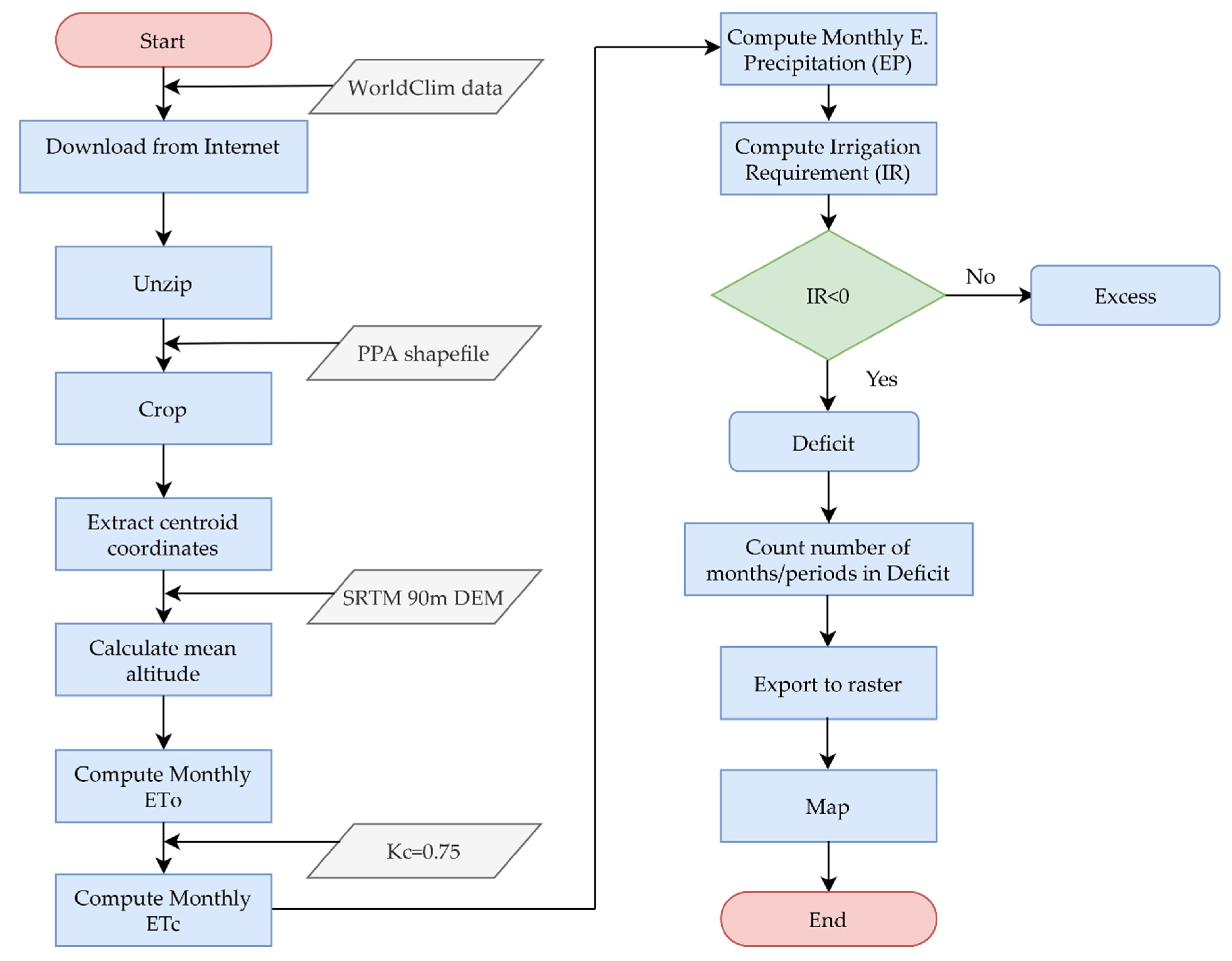
WC and ancillary data were downloaded from the sources mentioned in Table 1. Subsequently, a set of multi-step functions were coded in a script using R Software [39] to: (i) unzip and extract data from WC GeoTIFF images; (ii) crop WorldClim images to PPA limits (buffered at a distance of +500 m); (iii) extract centroid coordinates of each WorldClim pixel; (iv) calculate mean altitude of each WorldClim pixel from SRTM 90 m DEM; (iv) compute monthly reference evapotranspiration based on FAO-56 Penman-Monteith Equation (4); (vi) calculate crop evapotranspiration based on Equation (2); (vii) compute effective precipitation using WorldClim precipitation data; (viii) estimate the for each month (denote as in Equation (1)); (ix) classify each month according to value in “excess” (when ) or “deficit” (when ); (x) count the number of months and periods (individual and/or consecutive months) labeled as “deficit”, and (xi) export data in two raster stacks, the first one containing , , by month and the second including the number of months and the number and name (labeled as numeric classes) of those periods in water deficit. The workflow diagram is reported in Figure 2. QGIS software [41] was used to draw the water deficit maps, representing the spatial distribution of the number and the name of months/periods in water deficit in the PPA.
2.5. Model and Data Source Validation
Validation was carried out in three steps: (i) the first to compare the equation’s performance coded in an R Script, (ii) the second to correlate WC with weather observed stations (WS) data from the study area, and (iii) the third to measure WC data’s capability to predict months in water deficit and water excess. In the first step, values from the equation coded in the R script () were compared with values from the “Evapotranspiration” R package () (through function “ET.PenmanMonteith”) [42]. Both methods were tested using a 1280 daily climate dataset (1 March 2001–31 August 2004) from Kent Town Station in Adelaide (Australia), available in the “Evapotranspiration” R package. Root mean square error (RMSE), mean absolute error (MAE), coefficient of determination (with its corresponding significance test at 95% of confidence level), and a visual inspection on a graphic line 1:1 of vs. data were used to validate the coded equation. The motivation for coding the monthly equation (and its ancillary equations) instead of accumulating the daily from the R Package on a monthly basis is due to the differences between the daily and monthly equation. These differences are determined by soil heat flux () and the number of the day per year () [26]. In addition, is assumed as zero in the daily interval, and is the day of computation, while in the monthly interval, depends on the average temperature of the previous and subsequent months, and is the 15th day of the given month of computation.
In the second and third steps, WC data were validated annually (2015–2018) with monthly data from 73 WS [33], located in PPA, performing a linear regression and a categorical data analysis, respectively. After removing missing data from weather stations, months were reduced from 876 (73 stations by 12 months) to a maximum of 300, depending on the year analyzed. A monthly IR paired table (Equation (1)) was obtained from the spatially coincident WorldClim and weather station data. To standardize the number of months used by a given year, months from the paired table were randomly resampled (without replacement) 1000 times, extracting subsamples of 50 (deficit) and 50 (excess). A significance test (at 95% confidence level) was computed from the linear regression for each subsample, obtaining the coefficient of determination . Furthermore, months in deficit or excess from the paired table were compared in a 2 × 2 contingency table through McNemar’s test [43] to identify similarities (or differences) between the two data sources. Partial and global accuracy of WC data were calculated as the number of months correctly classified in deficit (cell (1,2) of the matrix) or excess (cell (2,1) of the matrix), and deficit and excess (sum of cells (2,1) and (2,1) of the matrix) between total analyzed months, respectively.
2.6. Computing the Location of Intertropical Convergence Zone and Its Influence on Irrigation Requirement
ITCZ geographic coordinates by month were obtained reading data from the netCDF format (functions nc_open and ncvar_get from R package ncdf4), computing for each (where ) the average of in the interval , computing for each the empirical cumulative distribution function (function “ecdf”), and calculating its inverse (function “quantile”). cells in that meet the condition of Equation (5) were labeled with one and those that were not at zero. Using the spatial resolution of , a raster was created, and then it was resampled to the spatial resolution of WorldClim data.
To estimate the influence of the ITCZ localization on the crop water deficit (IR), a relevance metric (RM) analysis was implemented using the Sensitivity Matrix method [44] over a supervised multilayer-perceptron artificial neural network (ANN) [45]. The influence was quantified by weighting the ITCZ-IR and Con-IR ANN optimized connections strength (product of RM analysis over the trained ANNs) and pondering the strength to a relative percentual weight. ANN was designed using an input layer with two neurons (two input variables, ITCZ, and a random control, Con), one hidden layer with a varied number of neurons (to be determined according to the correlation adjustment), and an output layer with one neuron (coincident with the output variable, IR). This was trained 500 times and tested by month using a random sample of 39,573 pixels (50% of the total), taken from a resampling of rasters IR, ITCZ, and random control (Con). The best ANN architecture was selected based on the lowest RMSE (accuracy to predict new observations) and standard deviation (stability among ANN with the same architecture). ANN modeling was performed using the R package “neuralnet” [46].
3. Results
3.1. Model and Data Source Validation
equations were validated with daily and monthly-extrapolated data. The regression analysis performed between these two datasets exposes high performance between the two computation methods. The MAE, the RMSE, and R2 between calculations, were , , and (), respectively. In addition, extrapolating to monthly data, MAE of was less than 2% (Figure 3).
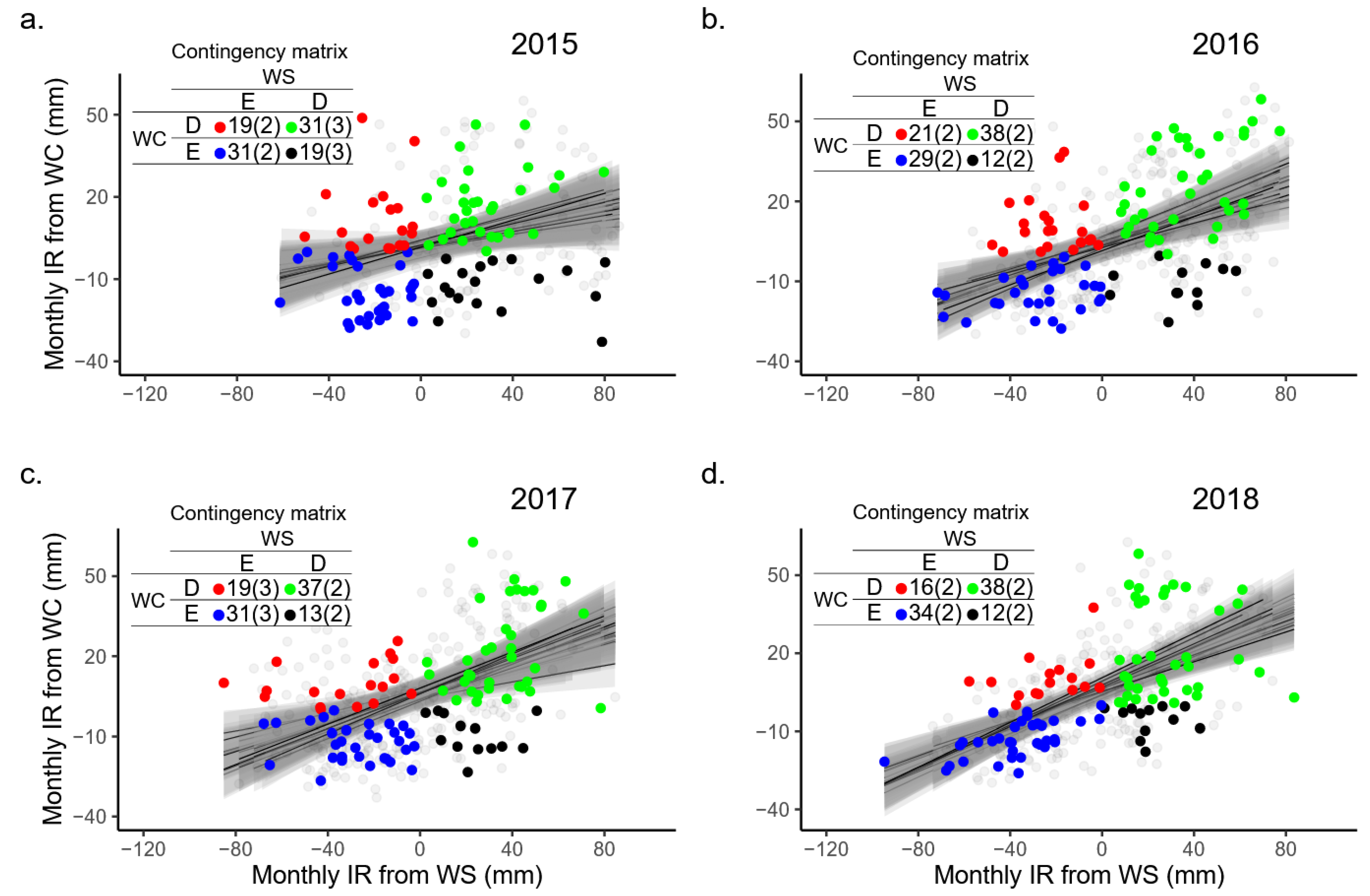
The filtering of WS missing data for the WC data validation resulted in a varied number of valid months per year. The year 2015 was the year with the fewest valid months (180 from 16 stations), while 2017 was the year with the most valid months (300 from 25 stations). The linear regression graph illustrates that the variability in from WS data is higher than that from WC data and the tendency of WC data to underestimate (Figure 3). The linear regression model computed has an average adjusted for the years 2015, 2016, 2017, and 2018 of , , , , respectively.
No significant differences were found (McNemar’s test, for all years analyzed) between months in deficit (D) or excess (E), classified by WC and WS data. The accuracy of WC to classify deficit months was 62, 76, 74, and 76% for the years 2015, 2016, 2017, and 2018, respectively (Figure 3). The global accuracy of the estimation using WC data was 60, 67, 68, and 72% for the years 2015 to 2018, respectively (Figure 3). According to the average contingency matrices presented in Figure 3, from 100 months tested, at least 62 were classified correctly (obtained by summing (1,2) and (2,1) contingency matrix’s cells).
3.2. Annual Distribution of Crop Evapotranspiration and Effective Precipitation
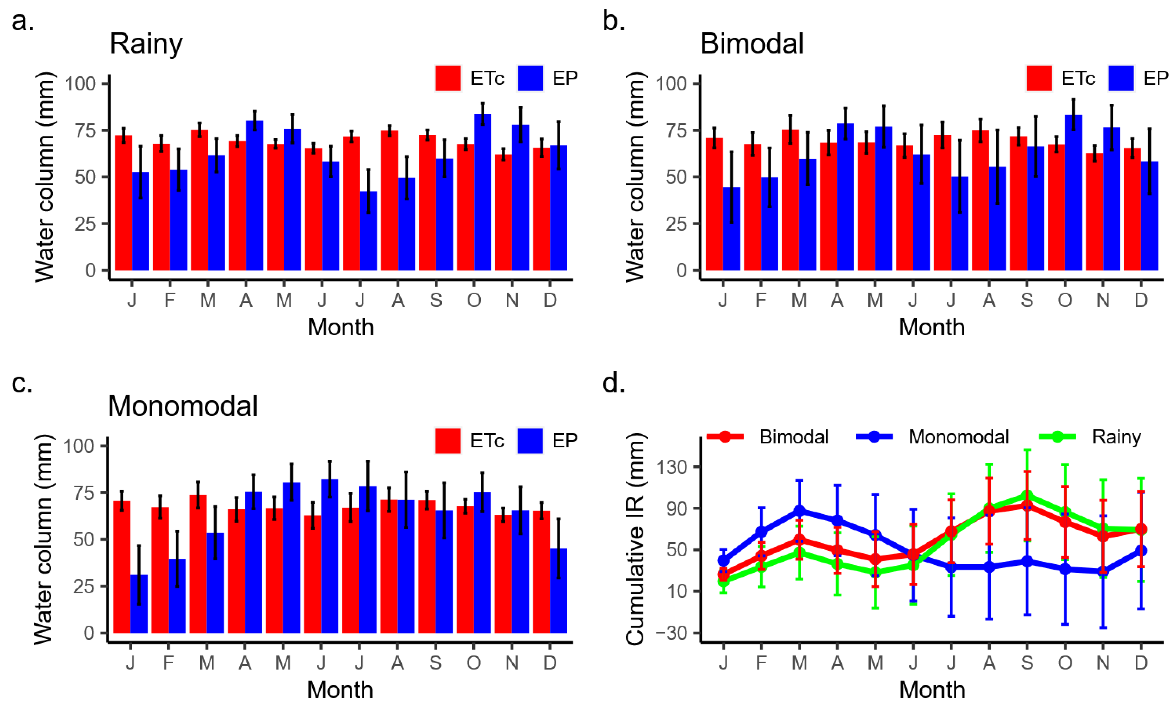
The annual distribution computed using WC data for the three precipitation regimes (Figure 4) was similar to that described in Colombia [35]. In the monomodal regime, May, June, and July are the rainiest months, while December, January, and February are the driest months (Figure 4a). In bimodal and rainy regimes, April, May, October, and November are the rainiest months, while January, February, July, and August are the driest months (Figure 4b,c). distributes homogeneously throughout the year in the three regimes with a slight increase in months when the decreases (Figure 4a–c).
The average and annual distribution in rainy and bimodal precipitation regimes of PPA (Figure 4a,b) allows us to see that, in the seven months with water deficit, exceeds from 8 to 69%. In the five months with water deficit in the monomodal regime (Figure 4c), exceeds by 1 to 128%. In those areas, Hass avocado could endure a water deficit of up to four months consecutively, accumulating on average a water deficit of up to 108 mm (Figure 4d).
The cumulative IR (Figure 4d) suggests that the rainfed Hass avocado orchards under bimodal and rainy precipitation regimes have one peak of water irrigation demand per semester: in March (60 and 47 mm, respectively) and in September (93 and 102 mm, respectively), while under the monomodal regime, the peak appears only in March (88 mm).
3.3. Water Deficit Visualizations under Geographic Space
Regarding computer performance, 79,145 pixels from WC and about 9.7 million pixels of SRTM 90 m GeoTIFF raster were processed using a set of functions coded in software R to output two raster stacks (pixel size 1 km2, spatially coincident with a WC pixel) in a total time of 1 h (Operative System Windows 10, processor Core I7 8700). Our results showed that January in the first semester and July and August in the second semester are the months where the highest percentage of PPA requires irrigation, while the fallen precipitation in April and October significantly reduces the area which requires irrigation (Table 2).
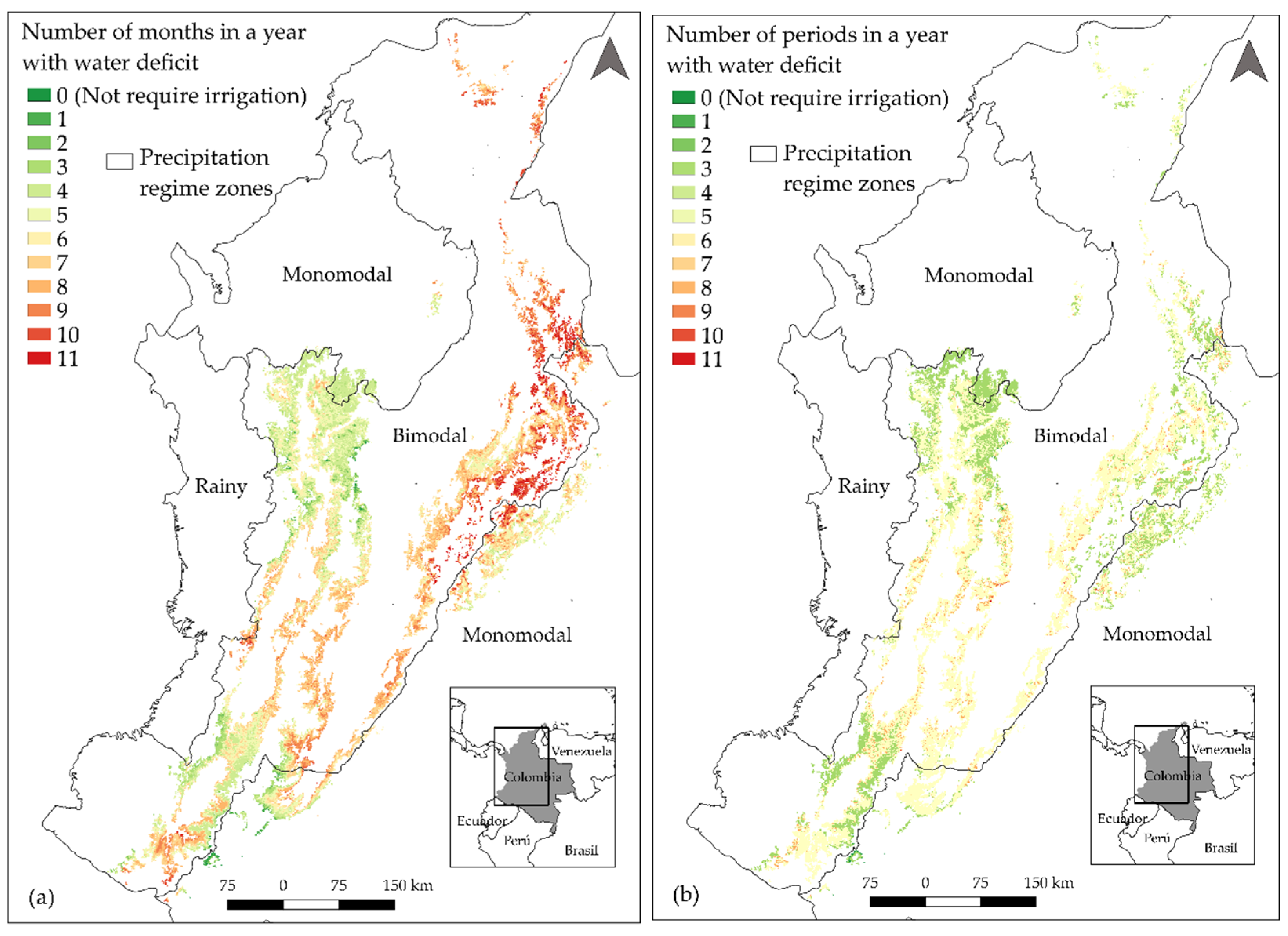
According to the water deficit maps (Figure 5), water deficit months fluctuate from zero (i.e., not require irrigation) to eleven (Figure 5a). Areas that do not require irrigation totalize 0.2% of PPA and are distributed in the northwest (Department of Antioquia) and the south of Colombia (Department of Putumayo). Areas that require irrigation from one to four months are in Antioquia, Caldas, Risaralda, Quindío, Cauca, and Huila departments. Zones that require irrigation in more than four months are distributed throughout the PPA, from the south to the north of Colombia, mainly in Departments of Cundinamarca, Boyacá, Santander, and Norte de Santander (Figure 5a). Areas that require irrigation at least one month in any given year account for 99.8% of the Hass avocado’s potential and current production area. The PPA percentages where avocado requires irrigation in bimodal, rainy, and monomodal regimes are 98.7, 100.0, and 99.4%, respectively.
Regarding these detailed periods, the water deficit associated to the Hass avocado cultivation in Colombia can be distributed in up to four periods in a year (Figure 5b). A total of 26.0% of PPA presents water deficit in one period (being December–March the most common) (Figure 5b). A total of 68.6% of PPA presents water deficit in two periods (being June–September and December–March the most common) (Figure 5b). Lastly, only 5.2% of PPA presents water deficit in three periods (with January, March, and June–September being the most common) (Figure 5b). Less than 0.1% of PPA presents water deficit in four periods (being January, March, June–September, and November the most common) (Figure 5b). Considering all four periods, December–March is the period where most PPA requires irrigation, with 8.7%.
3.4. Temporal and Spatial Variation of Irrigation Zones and Computing the Location of Intertropical Convergence Zone and Its Influence on Irrigation Requirement
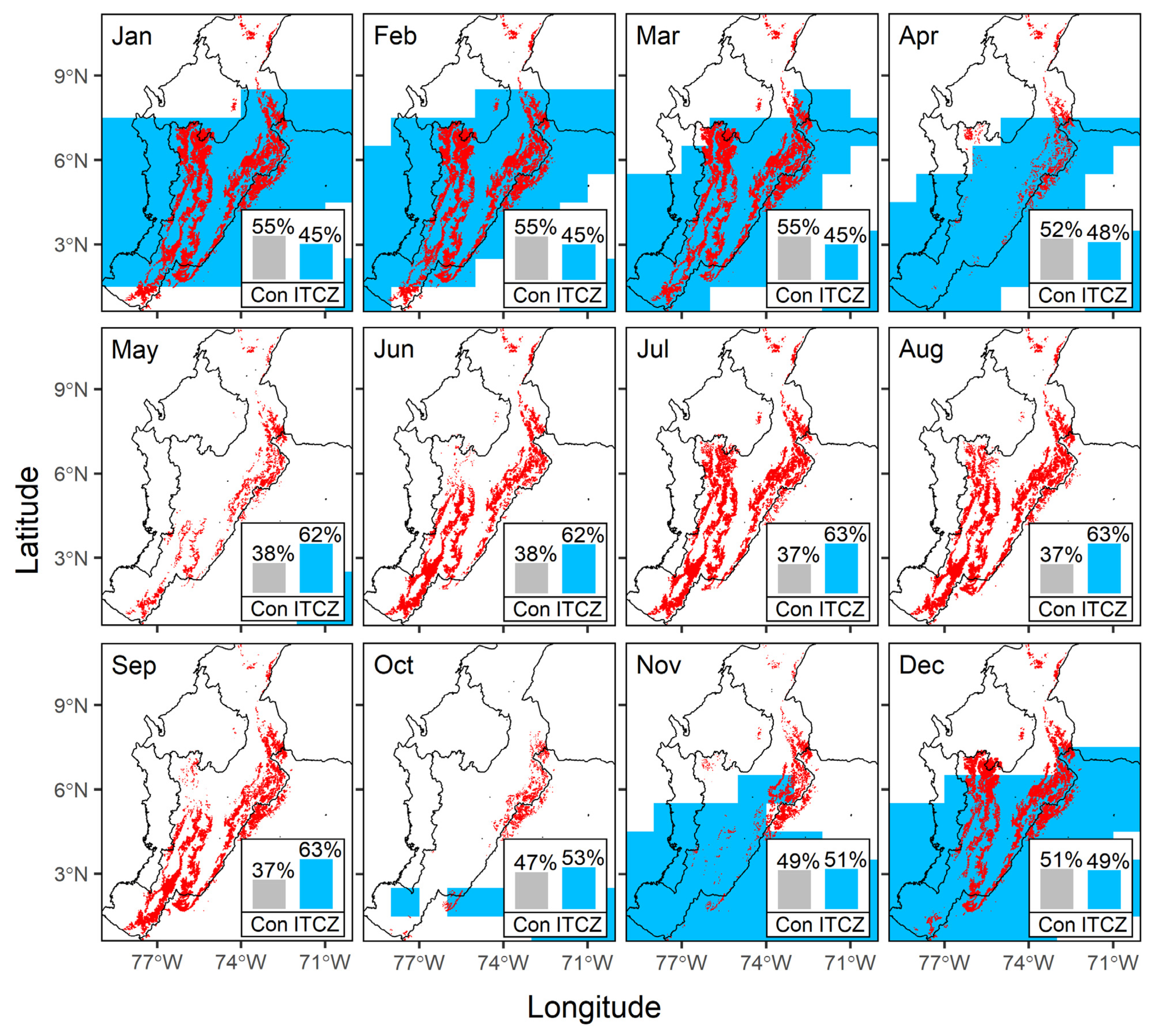
According to these results, the area to be irrigated at PPA changes spatial and temporally (Figure 6). From January to March, irrigation needs are distributed in all PPA, decreasing by 9.6%. In April and May, this area reduces significantly, decreasing from 81.5 (March) to 16.7% (May). From June to September, the IR area spreads in all PPA, July being the month with the highest area requiring irrigation, with 74.4% of PPA. From October to December, the IR area significantly increases, varying from 7.5 to 68.1% of PPA. Among the areas that require irrigation, the most and the less frequent months a year with irrigation deficit are January and April, and October, respectively (Figure 6).
The spatio-temporal dynamics of the water deficit area in PPA correspond to the variability of precipitation of the bimodal, monomodal, and rainy regimes. Two periods of water deficit (December–March and July–September) and two water excess periods (April–May and October–November) were found in the bimodal regime. In the monomodal regime, one period of water deficit (December to March) and one period of water excess (April to November) were found. Two periods of water deficit (January–February and July–August) and two water excess periods (March to June and September to December) were found in the rainy regime. Therefore, Figure 6 is consistent with Figure 4 because this illustrates a water deficit (i.e., when exceeds ) in the same months where PPA is affected by water deficit.
According to its resulting characteristics, ITCZ can be described as a globally distributed, longitudinal, and thin band that moves in Tropics from the north to the south, and vice versa throughout the year. The probability with which it was computed has a significant effect on the width of ITCZ. The higher probability, the thinner the ITCZ is. In continental South America, ITCZ at a 90% probability reaches its northernmost zone in January at 8.5° N, crossing the subcontinent from Colombia to French Guiana and its southernmost zone in July at 15.5° S, positioning itself on southern Colombia (Amazonas), Peru, Bolivia, and Brazil. In Colombia, ITCZ moves from the north to the south from January to April, covering no less than 82% of PPA (April). From May to September, ITCZ is out of PPA. ITCZ travels from the south to north in the remaining months, covering 83% of PPA in December (Figure 6).
After a processing time of 4.3 h, the backpropagation algorithm of all ANN converged and thus ANN were successfully trained. The number of neurons in the input, hidden, and output layers of the best ANN architecture of all months was 2, 20, and 1, respectively. RM analysis results (depicted in bar graphs inside the Figure 6 maps) suggest a high variability in ANN trained weights.
From November to April, the presence of ITCZ over PPA slightly influences the IR area, reaching a peak from January to March, when the influence is, on average, 10% lower than that on Con (Figure 6). The absence of ITCZ over PPA (May to October) behaves contrary to the presence, increasing the influence of ITCZ on the IR area. From May to September, ITCZ’s influence on IR is, on average, 26% higher than that on Con (Figure 6). The overall RM analysis (i.e., including all months that are not reported here) suggests the influence of ITCZ on IR, on average, is 4% higher than the influence of Con. Neither in the monthly nor annual RM analysis, the relative percentual weight of ITCZ was found to be significantly different from that of Con, according to the Wilcoxon signed-rank test ().
4. Discussion
4.1. Model and Data Source Validation
values resulting from the R Script equation had a significantly low MAE, RMSE, and agreed very well with those from the R Package equation, according to errors reported by [47] for hourly–daily comparison. Errors reported in this validation are acceptable in terms of their magnitude and thus do not affect the results’ effectiveness. Therefore, equations coded in the R script can be used to estimate in the model. Despite both equations having been obtained from the FAO-56 Penman-Monteith equation [26], reported errors are associated with the use of different coefficients, computation digits, and constants in ancillary equations by the two methods, as common sources of computation errors according to [48].
Results presented in this study suggest a moderately acceptable global accuracy in the validation of WorldClim data. Considering the origin (interpolation of global weather data) and period (1970 to 2000), validation of WorldClim data with current weather data in this study permit asserting that nowadays WorldClim data can be used to represent the irrigation requirement of Hass avocado cultivation in Colombia, corroborating validations in tropical mountainous regions [31]. To the extent of this study, it should be noted that this research paper is the first that uses WorldClim data (and reports its accuracy) in an irrigation requirement model. Despite the importance of secondary data validation to achieve more reliability in the results, papers referenced in this work that used WorldClim as input data of their models did not report accuracy.
The high variability of the monthly water balance model for the Hass avocado crop in Colombia proposed in this study concur with others developed globally, reported [49,50,51]. Limitations of the IR model proposed here are related to the omission of surface runoff, drainage, and upward flux from the soil water balance and the absence of inter-annual variation of WorldClim data. This omission is commonly reported in studies that computed soil water balance [52,53]. Allen et al. [26] established that the omission is due to these components are complex of measuring and do not significantly impact the SWB (in specific soil conditions). The absence of inter-annual variation is due to WorldClim data providing monthly climate data averaged in 1970–2000. Models that use WorldClim data to simulate environmental phenomena after 2000 did not report global and local interannual climate variability (El Niño–Southern Oscillation, ENSO).
To Hass avocado growers located in monomodal regime zones, who trigger the irrigation when the readily available water in the soil depletes [32], the magnitude of the maximum accumulated water deficit (Figure 4d) would be equal to stopping watering their orchards for up to three consecutive events. Basing ourselves on the cumulative IR in December (as do some Colombian farmers mentioned in the Introduction), which is low (79, 69, and 49 mm for bimodal, rainy, and monomodal regimes, respectively), Hass avocado orchards would not need irrigation because annual precipitation almost covers the total water that the crop requires, but distribution throughout the year and the spatial distribution of water deficit maps depict a very different scenario.
4.2. Water Deficit Visualization in Geographic Space
Water deficit maps demonstrate that although the annual distribution of precipitation in Colombia seems suitable for the avocado crop (Figure 4), a high percentage of the Hass avocado’s potential production area in Colombia needs water irrigation for at least one month per year (Figure 5 and Figure 6). This finding was similar in zones where a high amount of precipitation is distributed in one (monomodal regime) or two (bimodal regime) periods or throughout the year (rainy regime). It means farmers of Hass avocado in Colombia located in water deficit areas of bimodal, monomodal, and rainy precipitation regimes must irrigate their avocadoes to supply the crop’s water. Similar results were found in rice crops [54]. Although the total annual water rain in Bangladesh exceeded reference evapotranspiration (precipitation water varied from 1728 to 2776 mm, while varied from 1237 to 1364 mm), researchers estimated the average spatial net irrigation requirement was 676 mm (and in no case less than 400 mm). This indicates that the spatial distribution is a more accurate indicator to study irrigation requirements at a regional scale, as opposed to totalizing the annual amount of precipitation and evapotranspiration in the study area.
The water deficit maps are consistent with a study reported in Colombia [23], which comprised of a Hass avocado irrigation experiment in three farms located in Tolima, Antioquia, and Cauca (Colombia). Grajales [23] determined that even though the total annual precipitation was higher than the total annual reference evapotranspiration, a monthly distribution of these two variables showed exceeded precipitation in up to three months. After applying a treatment with an average of 12 drip irrigation events distributed in eight months per year, he reported a significant increase in the crop yield. Due to Hass avocado irrigation being a critical agronomic task to guarantee crop production success, water deficit maps become a powerful tool for Colombian farmers when scheduling irrigation in months and periods identified in these maps.
Moreover, water deficit maps can be used as a tool to design a strategy for redistributing and expanding crop areas according to the magnitude of water deficit. Steele et al. [55] computed a seasonal (May–September) evapotranspiration map (equivalent to water deficit map) in 2006 for more than ten crops in Devils Lake basin (USA) and determined seasonal evapotranspiration varied from 286 mm (dry edible beans) to approximately 611 mm (woods crop). After simulating increments of evapotranspiration in the evaluated crops by redistribution and expansion in the study area to mitigate flooding, a few suitable areas to accomplish this strategy were determined.
4.3. Influence on Irrigation Requirementof Intertropical Convergence Zone
Even though they both have different spatial and time resolutions, it can be observed that the spatial and temporal distribution of the computed ITCZ in this study is similar to those mapped, as reported [20,56]. Common characteristics between those are the bifurcation of IZCT in the eastern Pacific region and a predominant latitudinal displacement. Studies that relate global climate phenomena with agriculture (and particularly with irrigation) coincide with this in the existence of a significant relationship between these [57]. The given climate does not always trigger changes in the distribution of irrigated areas. Some large and densely irrigated regions (India, China, and USA) can drive changes in global climate [58]. The study of the influence of ITCZ on IR can become a tool to forecast adverse climate conditions and plan agronomic tasks to reduce the associated risks to the crops [59].
This study confirms the relationship between ITCZ and precipitation, described in Colombia’s monthly precipitation bulletins [60]. The movement of ITCZ toward latitudes far to those where PPA is located (i.e., when two areas do not intersect, May to September) decreases the precipitation, and therefore increases the Hass avocado area that requires irrigation. However, those bulletins also describe how other climate phenomena affect precipitation, leading to an integral model to improve the understanding of the problem. Among those factors that contributed to finding a slight influence of ITCZ on the Hass avocado irrigation requirement when areas intersect (October to April), we can consider the contrasting spatial resolution (pixel size) of the two data sources (which impede seeing spatial variability of ITCZ with more detail) and the difference between the periods in which data was obtained (WorldClim, 1970–2000 and ITCZ, 1932–2012).
Our study presents a latter-day tool for planning and decision-making in line with the Hass avocado cultivation sector in Colombia, as based on potential irrigation needs. Among the sources of variability evaluated associated with irrigation, a spatial and seasonal analysis (ITCZ) was presented. Other sources of variation that potentially affect requirements and availability of water in Hass avocado crops under tropical conditions, such as non-seasonal climate variability (ENSO) [4,57] and climate change [5], should be addressed in future works.
5. Conclusions
In this study, it is demonstrated that a high percentage of the current and potential production area of Hass avocado in Colombia needs water irrigation for at least one month per year. The performed analysis on zones with bimodal, monomodal, and rainy precipitation regimes in Colombia where Hass avocado can be potentially cultivated evidenced that there is a need for extra water in a high percentage of the area, not accounting for the precipitation regime. The approach of studying the irrigation requirement through its monthly spatial distribution is a more accurate indicator than studying this phenomenon at a regional scale, as it involves the totalizing of the annual amount of the precipitation and evapotranspiration in the study area. Water deficit maps have become a powerful tool for Colombian farmers when scheduling irrigation in months and periods as identified in the maps found in this study. Although the influence of the Intertropical Convergence Zone on the spatial distribution of Hass avocado irrigation requirements was higher than that obtained by a random variable in the second period of low precipitations (May to September), it is not possible to conclude that the Intertropical Convergence Zone has a significant influence on the spatial dynamics of irrigation requirement of the Hass avocado crop. This suggests that external climate phenomena contribute to the understanding of the spatial variability of irrigation requirements.
Author Contributions
Conceptualization, E.E.-M., J.G.R.-G., and A.E.S.; methodology, E.E.-M., J.G.R.-G., and A.E.S.; software, E.E.-M.; validation, E.E.-M.; formal analysis, E.E.-M.; investigation, E.E.-M. and A.E.S.; resources, E.E.-M. and A.E.S.; data curation, E.E.-M.; writing—original draft preparation, E.E.-M., J.G.R.-G., and A.E.S.; writing—review and editing, E.E.-M., J.G.R.-G., and A.E.S.; visualization, E.E.-M., J.G.R.-G., and A.E.S.; supervision, E.E.-M. and A.E.S.; project administration, E.E.-M. and A.E.S.; funding acquisition, E.E.-M., and A.E.S. All authors have read and agreed to the published version of the manuscript.
Funding
This research was supported by the Research Project BPIN 20140001100010 of National University of Colombia and the Research Group Regar, Facultad de Ingeniería, Universidad del Valle.
Institutional Review Board Statement
Not applicable.
Informed Consent Statement
Not applicable.
Data Availability Statement
The data presented in this study are available upon request from the corresponding author. The data are not publicly available due it being part of the research project and the group using the data for other analyses.
Conflicts of Interest
The authors declare no conflict of interest.
References
- FAOSTAT. Food and Agriculture Data. Available online: http://www.fao.org/faostat/en/#home (accessed on 4 February 2021).
- Serrano, A.; Brooks, A. Who is left behind in global food systems? Local farmers failed by Colombia’s avocado boom. Environ. Plan. E Nat. Space 2019, 2, 348–367. [Google Scholar] [CrossRef] [Green Version]
- Ramírez-Gil, J.G.; Morales, J.G.; Peterson, A.T. Potential geography and productivity of “Hass” avocado crops in Colombia estimated by ecological niche modeling. Sci. Hortic. 2018, 237, 287–295. [Google Scholar] [CrossRef]
- Ramírez-Gil, J.G.; Henao-Rojas, J.C. Mitigation of the Adverse Effects of the El Niño (El Niño, La Niña) Southern Oscillation (ENSO) Phenomenon and the Most Important Diseases in Avocado cv. Hass Crops. Plants 2020, 9, 790. [Google Scholar] [CrossRef]
- Ramírez-Gil, J.G.; Cobos, M.E.; Jiménez-García, D.; Morales-Osorio, J.G.; Peterson, A.T. Current and potential future distributions of Hass avocados in the face of climate change across the Americas. Crop Pasture Sci. 2019, 70, 694–708. [Google Scholar] [CrossRef]
- Nikolaou, G.; Neocleous, D.; Christou, A.; Kitta, E.; Katsoulas, N. Implementing Sustainable Irrigation in Water-Scarce Regions under the Impact of Climate Change. Agronomy 2020, 10, 1120. [Google Scholar] [CrossRef]
- Silva, S.R.D.; Cantuarias-Avilés, T.E.; Chiavelli, B.; Martins, M.A.; Oliveira, M.S. Phenological models for implementing management practices in rain-fed avocado orchards1. Pesqui. Agropecu. Trop. 2017, 47, 321–327. [Google Scholar] [CrossRef] [Green Version]
- Castillo-Argaez, R.; Schaffer, B.; Vazquez, A.; Sternberg, L.D.S.L. Leaf gas exchange and stable carbon isotope composition of redbay and avocado trees in response to laurel wilt or drought stress. Environ. Exp. Bot. 2020, 171. [Google Scholar] [CrossRef]
- Moreno-Ortega, G.; Pliego, C.; Sarmiento, D.; Barceló, A.; Martínez-Ferri, E. Yield and fruit quality of avocado trees under different regimes of water supply in the subtropical coast of Spain. Agric. Water Manag. 2019, 221, 192–201. [Google Scholar] [CrossRef]
- Silber, A.; Naor, A.; Cohen, H.; Bar-Noy, Y.; Yechieli, N.; Levi, M.; Noy, M.; Peres, M.; Duari, D.; Narkis, K.; et al. Irrigation of ‘Hass’ avocado: Effects of constant vs. temporary water stress. Irrig. Sci. 2019, 37, 451–460. [Google Scholar] [CrossRef]
- Ramírez-Gil, J.G.; López, J.H.; Henao-Rojas, J.C. Causes of hass avocado fruit rejection in preharvest, harvest, and packinghouse: Economic losses and associated variables. Agronomy 2020, 10, 8. [Google Scholar] [CrossRef] [Green Version]
- Hernández, I.; Fuentealba, C.; Olaeta, J.A.; Lurie, S.; Defilippi, B.G.; Campos-Vargas, R.; Pedreschi, R. Factors associated with postharvest ripening heterogeneity of “Hass” avocados (Persea americana Mill). Fruits 2016, 71, 259–268. [Google Scholar] [CrossRef] [Green Version]
- Kadbhane, S.J.; Manekar, V.L. Grape production assessment using surface and subsurface drip irrigation methods. J. Water Land Dev. 2021, 49, 169–178. [Google Scholar] [CrossRef]
- Kang, S.; Shin, Y.; Xie, S.-P. Extratropical forcing and tropical rainfall distribution: Energetics framework and ocean Ekman advection. Clim. Atmos. Sci. 2018, 1, 20172. [Google Scholar] [CrossRef] [Green Version]
- Mesa-Sánchez, Ó.J.; Rojo-Hernández, J.D. On the general circulation of the atmosphere around Colombia. Rev. Acad. Colomb. Cienc. Exactas Fis. Nat. 2020, 44, 857–875. [Google Scholar] [CrossRef]
- Takahashi, K.; Battisti, D.S. Processes controlling the mean tropical pacific precipitation pattern. Part I: The Andes and the eastern Pacific ITCZ. J. Clim. 2007, 20, 3434–3451. [Google Scholar] [CrossRef] [Green Version]
- Stephens, G.L.; Smalley, M.A.; Lebsock, M.D. The Cloudy Nature of Tropical Rains. J. Geophys. Res. Atmos. 2019, 124, 171–188. [Google Scholar] [CrossRef]
- Byrne, M.; Pendergrass, A.; Rapp, A.; Wodzicki, K. Response of the Intertropical Convergence Zone to Climate Change: Location, Width, and Strength. Curr. Clim. Chang. Rep. 2018, 4, 355–370. [Google Scholar] [CrossRef] [Green Version]
- Julich, S.; Mwangi, H.; Feger, K.-H. Forest Hydrology in the Tropics. In Tropical Forestry Handbook; Pancel, L., Köhl, M., Eds.; Springer: Berlin/Heidelberg, Germany, 2016; pp. 1917–1939. [Google Scholar]
- Mamalakis, A.; Foufoula-Georgiou, E. A Multivariate Probabilistic Framework for Tracking the Intertropical Convergence Zone: Analysis of Recent Climatology and Past Trends. Geophys. Res. Lett. 2018, 45, 13080–13089. [Google Scholar] [CrossRef]
- Richter, M. Precipitation in the Tropics. In Tropical Forestry Handbook; Pancel, L., Köhl, M., Eds.; Springer: Berlin/Heidelberg, Germany, 2016; pp. 363–390. [Google Scholar]
- González-Orozco, C.E.; Porcel, M.; Alzate Velásquez, D.F.; Orduz-Rodríguez, J.O. Extreme climate variability weakens a major tropical agricultural hub. Ecol. Indic. 2020, 111, 106015. [Google Scholar] [CrossRef]
- Grajales, L. Uso Racional del Agua de Riego en Cultivo de Aguacate Hass (Persea Americana) en tres Zonas Productoras de Colombia; Universidad Nacional de Colombia: Bogotá, Colombia, 2017. [Google Scholar]
- NRCS Water Requirements. National Engineering Handbook: Irrigation Guide. Part 652; United States Department of Agriculture: Washington, DC, USA, 1997; p. 754. [Google Scholar]
- Bos, M.; Kselik, R.; Allen, R.; Molden, D. Water Requirements for Irrigation and the Environment; Springer: Dordrecht, The Netherlands, 2009; ISBN 978-1-4020-8947-3. [Google Scholar]
- Allen, R.; Pereira, L.; Raes, D.; Smith, M. FAO Irrigation and Drainage Paper No. 56: Crop Evapotranspiration (Guidelines for Computing Water Requirements); Food and Agriculture Organization of the United Nations: Rome, Italy, 1998. [Google Scholar]
- Ali, M. Field Water Balance. In Fundamentals of Irrigation and On-Farm Water Management; Springer: Mymensingh, Bangladesh, 2010; Volume 1, pp. 331–372. ISBN 9781441963345. [Google Scholar]
- Carr, M.K.V. The water relations and irrigation requirements of avocado (Persea americana Mill.): A review. Exp. Agric. 2013, 49, 256–278. [Google Scholar] [CrossRef]
- Silber, A.; Israeli, Y.; Levi, M.; Keinan, A.; Shapira, O.; Chudi, G.; Golan, A.; Noy, M.; Levkovitch, I.; Assouline, S. Response of “Hass” avocado trees to irrigation management and root constraint. Agric. Water Manag. 2012, 104, 95–103. [Google Scholar] [CrossRef]
- Holzapfel, E.; de Souza, J.A.; Jara, J.; Guerra, H.C. Responses of avocado production to variation in irrigation levels. Irrig. Sci. 2017, 35, 205–215. [Google Scholar] [CrossRef]
- Fick, S.E.; Hijmans, R.J. WorldClim 2: New 1-km spatial resolution climate surfaces for global land areas. Int. J. Climatol. 2017, 37, 4302–4315. [Google Scholar] [CrossRef]
- UPRA. Zonificación de Aptitud Para el Cultivo Comercial de Aguacate Hass en Colombia, a Escala 1:100.000; Ministerio de Agricultura y Desarrollo Rural: Bogotá, Colombia, 2018. [Google Scholar]
- IDEAM. Consulta y Descarga de Datos Hidrometeorológicos. Available online: http://dhime.ideam.gov.co/atencionciudadano/ (accessed on 4 July 2019).
- Ballabio, C.; Borrelli, P.; Spinoni, J.; Meusburger, K.; Michaelides, S.; Beguería, S.; Klik, A.; Petan, S.; Janeček, M.; Olsen, P.; et al. Mapping monthly rainfall erosivity in Europe. Sci. Total Environ. 2017, 579, 1298–1315. [Google Scholar] [CrossRef] [PubMed] [Green Version]
- Guzmán, D.; Ruíz, J.F.; Cadena, M. Regionalización de Colombia según la Estacionalidad de la Precipitación Media Mensual, a Través Análisis de Componentes Principales (ACP); IDEAM: Bogotá, Colombia, 2014. [Google Scholar]
- Lee, H.-T. Program NOAA CDR NOAA Climate Data Record (CDR) of Monthly Outgoing Longwave Radiation (OLR), Version 2.2-1. Available online: https://data.nodc.noaa.gov/cgi-bin/iso?id=gov.noaa.ncdc:C00809# (accessed on 16 May 2020).
- WorldClim. Historical Climate Data. Available online: https://www.worldclim.org/data/worldclim21.html (accessed on 15 January 2020).
- CGIAR. SRTM 90m Digital Elevation Database. Available online: https://bigdata.cgiar.org/srtm-90m-digital-elevation-database/ (accessed on 8 July 2021).
- R Core Team. R: A Language and Environment for Statistical Computing, Vienna, Austria. 2020. Available online: https://www.R-project.org (accessed on 15 September 2020).
- NOAA. NOAA Interpolated Outgoing Longwave Radiation (OLR). Available online: https://psl.noaa.gov/data/gridded/data.interp_OLR.html (accessed on 14 May 2020).
- QGIS. Development Team QGIS Geographic Information System. 2020. Available online: http://qgis.org (accessed on 1 August 2020).
- Guo, D.; Peterson, T. Package Evapotranspiration: Modelling Actual, Potential and Reference Crop Evapotranspiration. 2020. Available online: https://cran.r-project.org/package=evapotranspiration (accessed on 20 September 2020).
- Agresti, A. Contingency Tables. In An Introduction to Categorical Data Analysis; John Wiley & Sons: Gainesville, FL, USA, 2007; pp. 21–64. [Google Scholar]
- Satizábal, H.; Pérez-Uribe, A. Relevance Metrics to Reduce Input Dimensions in Artificial Neural Networks. In Artificial Neural Networks—ICANN 2007; Marques de Sá, J., Alexandre, L., Duch, W., Mandic, D., Eds.; Springer: Porto, Portugal, 2007; pp. 39–48. ISBN 978-3-540-74690-4. [Google Scholar]
- Galushkin, A. Neural Networks Theory; Springer: Berlin/Heidelberg, Germany, 2007; ISBN 978-3-540-48125-6. [Google Scholar]
- Fritsch, S.; Guenther, F.; Wright, M.; Suling, M.; Mueller, S. Package “Neuralnet”: Training of Neural Networks. 2019. Available online: https://cran.r-project.org/package=neuralnet (accessed on 3 July 2019).
- Djaman, K.; Irmak, S.; Sall, M.; Sow, A.; Kabenge, I. Comparison of sum-of-hourly and daily time step standardized ASCE Penman-Monteith reference evapotranspiration. Theor. Appl. Climatol. 2018, 134, 533–543. [Google Scholar] [CrossRef]
- Allen, R.; Pereira, L.S.; Howell, T.A.; Jensen, M.E. Evapotranspiration information reporting: I. Factors governing measurement accuracy. Agric. Water Manag. 2011, 98, 899–920. [Google Scholar] [CrossRef] [Green Version]
- Elnashar, A.; Wang, L.; Wu, B.; Zhu, W.; Zeng, H. Synthesis of global actual evapotranspiration from 1982 to 2019. Earth Syst. Sci. Data 2021, 13, 447–480. [Google Scholar] [CrossRef]
- Trabucco, A.; Zomer, R. Global High-Resolution Soil-Water Balance. Available online: https://cgiarcsi.community/data/global-high-resolution-soil-water-balance/ (accessed on 8 July 2021).
- Zhuang, W.; Shi, H.; Ma, X.; Cleverly, J.; Beringer, J.; Zhang, Y.; He, J.; Eamus, D.; Yu, Q. Improving Estimation of Seasonal Evapotranspiration in Australian Tropical Savannas using a Flexible Drought Index. Agric. For. Meteorol. 2020, 295, 108203. [Google Scholar] [CrossRef]
- Han, M.; Zhang, H.; Chávez, J.L.; Ma, L.; Trout, T.J.; DeJonge, K.C. Improved soil water deficit estimation through the integration of canopy temperature measurements into a soil water balance model. Irrig. Sci. 2018, 36, 187–201. [Google Scholar] [CrossRef]
- Garrido-Rubio, J.; Sanz, D.; González-Piqueras, J.; Calera, A. Application of a remote sensing-based soil water balance for the accounting of groundwater abstractions in large irrigation areas. Irrig. Sci. 2019, 709–724. [Google Scholar] [CrossRef]
- Mainuddin, M.; Kirby, M.; Chowdhury, R.A.R.; Shah-Newaz, S.M. Spatial and temporal variations of, and the impact of climate change on, the dry season crop irrigation requirements in Bangladesh. Irrig. Sci. 2015, 33, 107–120. [Google Scholar] [CrossRef]
- Steele, D.D.; Thoreson, B.P.; Hopkins, D.G.; Clark, B.A.; Tuscherer, S.R.; Gautam, R. Spatial mapping of evapotranspiration over Devils Lake Basin with SEBAL: Application to flood mitigation via irrigation of agricultural crops. Irrig. Sci. 2015, 33, 15–29. [Google Scholar] [CrossRef]
- Adam, O.; Bischoff, T.; Schneider, T. Seasonal and interannual variations of the energy flux equator and ITCZ. Part I: Zonally averaged ITCZ position. J. Clim. 2016, 29, 3219–3230. [Google Scholar] [CrossRef]
- Barrios-Perez, C.; Okada, K.; Varón, G.G.; Ramirez-Villegas, J.; Rebolledo, M.C.; Prager, S.D. How does El Niño Southern Oscillation affect rice-producing environments in central Colombia? Agric. For. Meteorol. 2021, 306. [Google Scholar] [CrossRef]
- Guimberteau, M.; Laval, K.; Perrier, A.; Polcher, J. Global effect of irrigation and its impact on the onset of the Indian summer monsoon. Clim. Dyn. 2012, 39, 1329–1348. [Google Scholar] [CrossRef]
- Meza, F. Use of ENSO-Driven Climatic Information for Optimum Irrigation under Drought Conditions: Preliminary Assessment Based on Model Results for the Maipo River Basin, Chile. In Climate Prediction and Agriculture: Advances and Challenges; Sivakumar, M., Hansen, J., Eds.; Springer: Berlin/Heidelberg, Germany,, 2007; pp. 79–88. ISBN 9781626239777. [Google Scholar]
- IDEAM. Boletín Hidroclimatológico Mensual. Available online: http://www.ideam.gov.co/web/tiempo-y-clima/climatologico-mensual (accessed on 2 March 2021).
Figure 1.
Distribution of Colombia’s current and potential Hass avocado production zones (PPA), according to precipitation regimes zones.
Figure 1.
Distribution of Colombia’s current and potential Hass avocado production zones (PPA), according to precipitation regimes zones.

Figure 2.
Flux diagram of IR computation.

Figure 3.
Validation of monthly IR from WorldClim (WC) using Weather Stations (WS) data from: (a) year 2015; (b) year 2016; (c) year 2017; and (d) year 2018. Colored points represent one of the coincident subsamples with the average contingency matrix (in parenthesis standard deviation). Gray points represent other subsamples.

Figure 4.
Average annual distribution of
(effective precipitation),
(crop evapotranspiration) at PPA (potential production area in Colombia) in: (a) rainy; (b) bimodal; and (c) monomodal precipitation regimes, and (d) the cumulative IR (irrigation requirement). Error bars correspond to absolute (panels (a) to (c)) and cumulative (panel (d)) standard deviation.

Figure 5.
Spatiotemporal distribution of water deficit a year in PPA (potential production area in Colombia) represented with a pixel size of 1 km2. (a) Number of months in water deficit; (b) number of periods in water deficit.
Figure 5.
Spatiotemporal distribution of water deficit a year in PPA (potential production area in Colombia) represented with a pixel size of 1 km2. (a) Number of months in water deficit; (b) number of periods in water deficit.

Figure 6.
Spatiotemporal distribution of the area that requires irrigation in PPA and the relative percentual weight of ITCZ location (blue) on IR in comparison to a control variable (Con, gray) product of the relevance metric analysis.
Figure 6.
Spatiotemporal distribution of the area that requires irrigation in PPA and the relative percentual weight of ITCZ location (blue) on IR in comparison to a control variable (Con, gray) product of the relevance metric analysis.


Table 1.
Description of variables used in the study.
| Variable Name | Units | Format | Source |
|---|---|---|---|
| Hass Avocado’s Potential production area in Colombia | m2 | Shapefile | Datos Abiertos (https://www.datos.gov.co/) (accessed on 10 December 2019) [32] |
| Solar radiation | KJ m−2 day−1 | GeoTIFF | WorldClim (https://www.worldclim.org/) (accessed on 15 January 2020) [37] |
| Maximum temperature | °C | GeoTIFF | WorldClim (https://www.worldclim.org/) |
| Minimum temperature | °C | GeoTIFF | WorldClim (https://www.worldclim.org/) |
| Average temperature | °C | GeoTIFF | WorldClim (https://www.worldclim.org/) |
| Wind speed | m s−1 | GeoTIFF | WorldClim (https://www.worldclim.org/) |
| Water vapor pressure | kPa | GeoTIFF | WorldClim (https://www.worldclim.org/) |
| Precipitation | mm | GeoTIFF | WorldClim (https://www.worldclim.org/) |
| Altitude | m | GeoTIFF | SRTM 90 m (http://srtm.csi.cgiar.org/) (accessed on 8 July 2021) [38] |
| Day of year | DOY | dd-mm-yy | R function lubridate::days_in_month(…) [39] |
| Geographic coordinates | Decimal degrees | dd.ddddd | Centroid of WorldClim pixels |
| Outgoing Longwave Radiation | W m−2 | netCDF | NOAA (https://www.ncdc.noaa.gov/) (accessed on 14 May 2020) [40] |
Table 2.
Area classified in water deficit in PPA (potential production area in Colombia) by month (km2).
Table 2.
Area classified in water deficit in PPA (potential production area in Colombia) by month (km2).
| Regime | Jan | Feb | Mar | Apr | May | Jun | Jul | Aug | Sep | Oct | Nov | Dec |
|---|---|---|---|---|---|---|---|---|---|---|---|---|
| Bimodal | 58,804 | 54,864 | 53,652 | 7061 | 12,085 | 40,371 | 56,086 | 52,805 | 38,283 | 3174 | 9186 | 42,129 |
| Rainy | 291 | 302 | 304 | 18 | 69 | 290 | 331 | 321 | 304 | 1 | 16 | 161 |
| Monomodal | 13,045 | 12,342 | 10,555 | 1926 | 1070 | 376 | 2455 | 5666 | 8803 | 2772 | 5315 | 11,636 |
| Total | 72,140 | 67,508 | 64,511 | 9005 | 13,224 | 41,037 | 58,872 | 58,792 | 47,390 | 5947 | 14,517 | 53,926 |
| Percentage | 91.1 | 85.3 | 81.5 | 11.4 | 16.7 | 51.9 | 74.4 | 74.3 | 59.9 | 7.5 | 18.3 | 68.1 |
Publisher’s Note: MDPI stays neutral with regard to jurisdictional claims in published maps and institutional affiliations. |
© 2021 by the authors. Licensee MDPI, Basel, Switzerland. This article is an open access article distributed under the terms and conditions of the Creative Commons Attribution (CC BY) license (https://creativecommons.org/licenses/by/4.0/).
Share and Cite
MDPI and ACS Style
Erazo-Mesa, E.; Ramírez-Gil, J.G.; Sánchez, A.E. Avocado cv. Hass Needs Water Irrigation in Tropical Precipitation Regime: Evidence from Colombia. Water 2021, 13, 1942. https://doi.org/10.3390/w13141942
AMA Style
Erazo-Mesa E, Ramírez-Gil JG, Sánchez AE. Avocado cv. Hass Needs Water Irrigation in Tropical Precipitation Regime: Evidence from Colombia. Water. 2021; 13(14):1942. https://doi.org/10.3390/w13141942
Chicago/Turabian StyleErazo-Mesa, Edwin, Joaquín Guillermo Ramírez-Gil, and Andrés Echeverri Sánchez. 2021. "Avocado cv. Hass Needs Water Irrigation in Tropical Precipitation Regime: Evidence from Colombia" Water 13, no. 14: 1942. https://doi.org/10.3390/w13141942
Note that from the first issue of 2016, this journal uses article numbers instead of page numbers. See further details here.