Estimation of the G2P Design Storm from a Rainfall Convectivity Index

Abstract

The two-parameter gamma function (G2P) design storm is a recent methodology used to obtain synthetic hyetographs especially developed for urban hydrology applications. Further analytical developments on the G2P design storm are presented herein, linking the rainfall convectivity n-index with the shape parameter of the design storm. This step can provide a useful basis for future easy-to-handle rainfall inputs in the context of regional urban drainage studies. A practical application is presented herein for the case of Valencia (Spain), based on high-resolution time series of rainfall intensity. The resulting design storm captures certain internal statistics and features observed in the fine-scale rainfall intensity historical records. On the other hand, a direct, simple method is formulated to derivate the design storm from the intensity–duration–frequency (IDF) curves, making use of the analytical relationship with the n-index.

1. Introduction

Floods have increased within the last century in many parts of the world due to a combination of factors with different levels of impact depending on the level of development of each region [1]. In Europe, as in other developed areas, one of the main factors contributing to the increase in this type of risk lays on the traditional configuration of cities, in which large areas of land have been sealed during urbanization, reducing infiltration. In addition, different authors have been warning for more than a decade that in the near future, an increase in rainfall intensity is expected [2,3,4]. In coastal areas with maritime influence, as it is the case in the Mediterranean, the problem is worsened because an increase in sea temperature can increase the frequency of extreme rainfall events [5,6]. Therefore, many urban drainage networks have to cope today with heavier rainfall inputs in a more sealed urban environment. The consequence is a greater runoff production that may collapse the urban drainage system. Urban hydrology has to face the challenges derived from this evolving situation in our cities. In urban areas, where many catchments are small with short times of concentration, it is important to adapt stormwater drainage systems to these changes in rainfall intensities in order to prevent urban floods [7,8]. Thus, urban hydrological models are essential tools to diagnose the system response and to define and design the needed hydraulic infrastructures. To this end, the use of design storms is of great interest for urban hydrology applications.

Most of the design storms available in the literature emerged between the 1970s and 1980s of the last century with the aim of reducing design uncertainty by introducing a synthetic rainfall as input of hydrological simulation models. Design storms can be sorted in two categories. On the one hand, there are those obtained straight from IDF curves. These methods base their construction either on a point on the IDF curve to which they associate different geometric shapes or on the entire IDF curve. Under the first group, we can find the rectangular [9], triangular [10], Sifalda [11], double triangle [12] or linear/exponential [13] design storms. The Chicago design storm [14] or the alternating block method [15] are examples basing their construction on the entire IDF curve. On the other hand, we can find synthetic design storms derived from observed precipitation patterns, as it is the case of the Illinois State Water Survey (ISWS) storm [16], the National Resources Conservation Services (NRCS) storm [17], the average variability method (AVM) [18] or the more recent two-parameter gamma function (G2P) design storm [19]. Regarding this second category, many of these design storms associate a temporal distribution based on observed real precipitation data to a precipitation volume obtained from the IDF curve, thus providing a more realistic temporal distribution.

The G2P design storm [19] was developed as a new tool for designing urban infrastructures under convective rainfall events, such as in the Mediterranean coastline of the Valencian Region (Spain). One of the main achievements of the G2P design storm is to represent in a set of hyetographs for a given return period the most likely pairs of maximum rainfall intensity and event rainfall depth, for short periods of time representative of convective storms.

The G2P design storm was compared with other well-known design storm methodologies [20]. The study highlighted two advantages of the G2P design storm. First, the possibility of assigning a set of rainfall temporal patterns to a single return period. This possibility enriches the hydrological analysis, since not all hydraulic elements within the system will respond in the same way to a given rainfall shape. Indeed, most conditioning storm parameters for a hydraulic design are not only rainfall intensities but also storm duration, total rainfall depth and temporal structure of the storm, as it is the case when designing storm tanks or sustainable urban drainage systems. Secondly, the possibility of regionalising the model parameters, as a consequence of its compact analytical formulation, is based on two parameters. This simple formulation eases the systematic statistical treatment for regional analysis, allowing for the regionalization of the model parameters for the characterization of G2P design storms for urban hydrology applications.

Despite its advantages, the G2P design storm has still to overcome some difficulties before becoming a mainstream method. The need to analyse long historical rainfall series for estimating the model parameters makes it difficult to estimate its parameters.

To overcome such inconvenience, simpler procedures to estimate the two parameters are proposed in this research, adapted to practical applications with no availability of high-resolution rainfall records.

The paper presents an analytical relationship relating the shape parameter of the G2P design storm with a convenient index of rainfall convectivity. Then, a simple procedure is proposed to establish a relationship between the scale parameter of the G2P design storm and the IDF curves. The procedures are illustrated with an application performed with rainfall data from Valencia (Spain).

2. Rainfall Characterization

2.1. Selection of an Irregularity Index for the Storm Temporal Structure

An accurate representation of the temporal structure of precipitation is, among other aspects, related to the storm magnitude, essential to design hydraulic infrastructures efficiently. The most usual way of describing time dependent intensities is by means of design storms. If historical records of enough temporal resolution are available, hyetographs are obtained from observed series of precipitation to reproduce a better approximation to the real phenomenon. However, this is not always possible, and many design storms are derived from statistical characterizations of maximum average intensities for different time scales to which a frequency or return period is associated (IDF curves). Nevertheless, the temporal structure may vary according to the selected storm duration and IDF parameters, as [21] demonstrated when using the Sherman equation, one of the most widely used IDF curve.

The lack of data with sufficient temporal resolution to approximate the real temporal structure of precipitation is often solved by means of stochastic generation of sequences of sub-daily rainfall [22,23,24,25,26]. Other authors used the fractal theory in which, considering the self-similarity of precipitation, the rainfall scale properties may improve the characterization of IDF curves. Vašková [27] applied the fractal analysis for IDF curves estimation using historical data series from Barcelona and Valencia (Spain), both located on the Mediterranean coast where high torrential intensities are frequent. Similarly, García-Marín [28] analysed the multifractal characteristics of precipitation according to the observation scale in Andalucía (Spain), relating this scale to IDF curves.

An alternative approach to describe the rainfall temporal evolution is based on estimating descriptive indices of rainfall intra-event irregularity. Martín-Vide [29] and Maraun et al. [30] established several indices that classify precipitation according to its annual distribution. Other indices characterize the temporal irregularity of rainfall by quantifying its convective properties. The advantage of these indices over the former is their meteorological rather than climatic character. Three different examples of this type of indices are the β-index [31], the Precipitation Index (IP), [32] and the n-index [33].

The β-index [31] quantifies the rainfall convectivity by means of an expression based on a threshold that varies depending on the temporal aggregation level. This index was developed for the climatic region in north-eastern Spain.

The Precipitation Index (IP) [32] resembles the β-index as it seeks for setting the convective fraction of rainfall according to its relative intensity. It is a weighted index of the maximum intensities of 5 min, 1, 2 and 24 h, as they are representative durations of different scales in the origin of rainfall. The IP index was derived from a statistical analysis in the same study area than the one used in the above described β-index.

Finally, the n-index method [34,35] describes the temporal intra-event structure of rainfall using a dimensionless index relating the potential relationship between two maximum intensities corresponding to different temporal intervals within the storm. This method allows us to describe the temporal distribution of any type of precipitation as a function of the n-index, regardless the total amount of cumulative precipitation.

The author of the n-index discussed all the previous indices, concluding that the n-index presents some advantages over the previous ones [34]. First, the n-index removes the arbitrary introduction of thresholds, as 0 ≤ n ≤ 1. In addition, its possible definition for different time scales makes it versatile for different study approaches. Indeed, the n-index is consistent with the fractal dimension of the rainfall intensity. This property allows the study of any typical rainfall temporal pattern worldwide by means of the n-index.

After reviewing the different existing methodologies and indices to characterize the temporal distribution of rainfall, the n-index has been selected to relate the rainfall temporal pattern to the G2P design storm parameters. The potential relation used to characterize intra-event distribution of intensities (see Section 2.2) and the physical meaning of the n-index related to the convective character of rainfall make this method feasible to achieve the objective of this research.

2.2. Rainfall Data

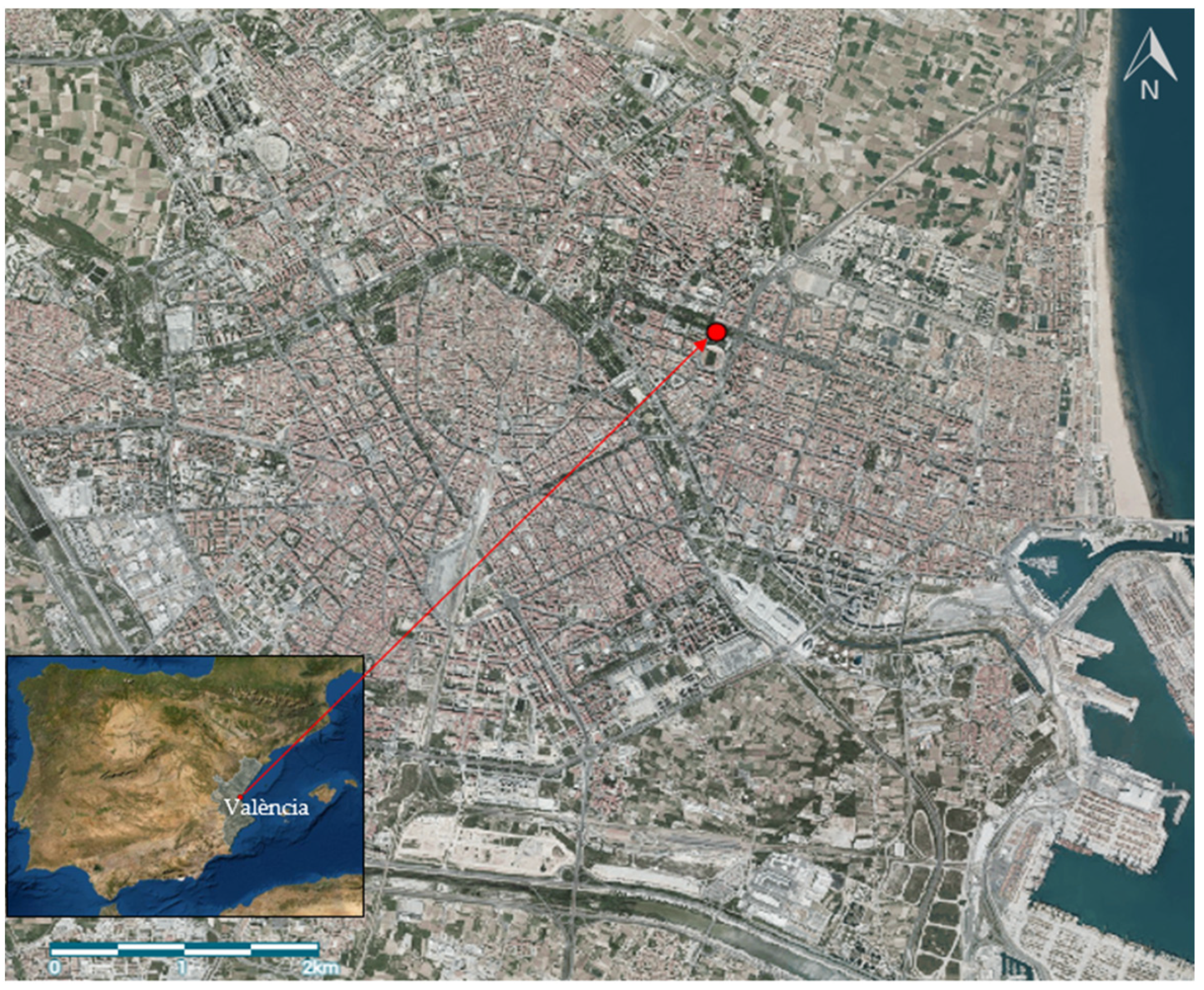
The rainfall data series used in this research come from the automatic rain gauge located in Valencia city (39°28′35″ N; 0°21′28″ W, altitude 25 m), Spain (Figure 1). Valencia presents a combination of Csa and Bsh types of climate according to the Köppen–Geiger climate classification [36]. It is characterized by a semiarid Mediterranean climate with mean annual temperatures around 17.5 °, mild winter and hot and dry summer. The average annual maximum rainfall is 495 mm, irregularly distributed between seasons. Daily rainfall values over 200 mm have been recorded during the autumn season, due to the effect of cut-off lows in this area, strongly influenced by the highest values of the Mediterranean Sea surface temperature reached during September and October months.

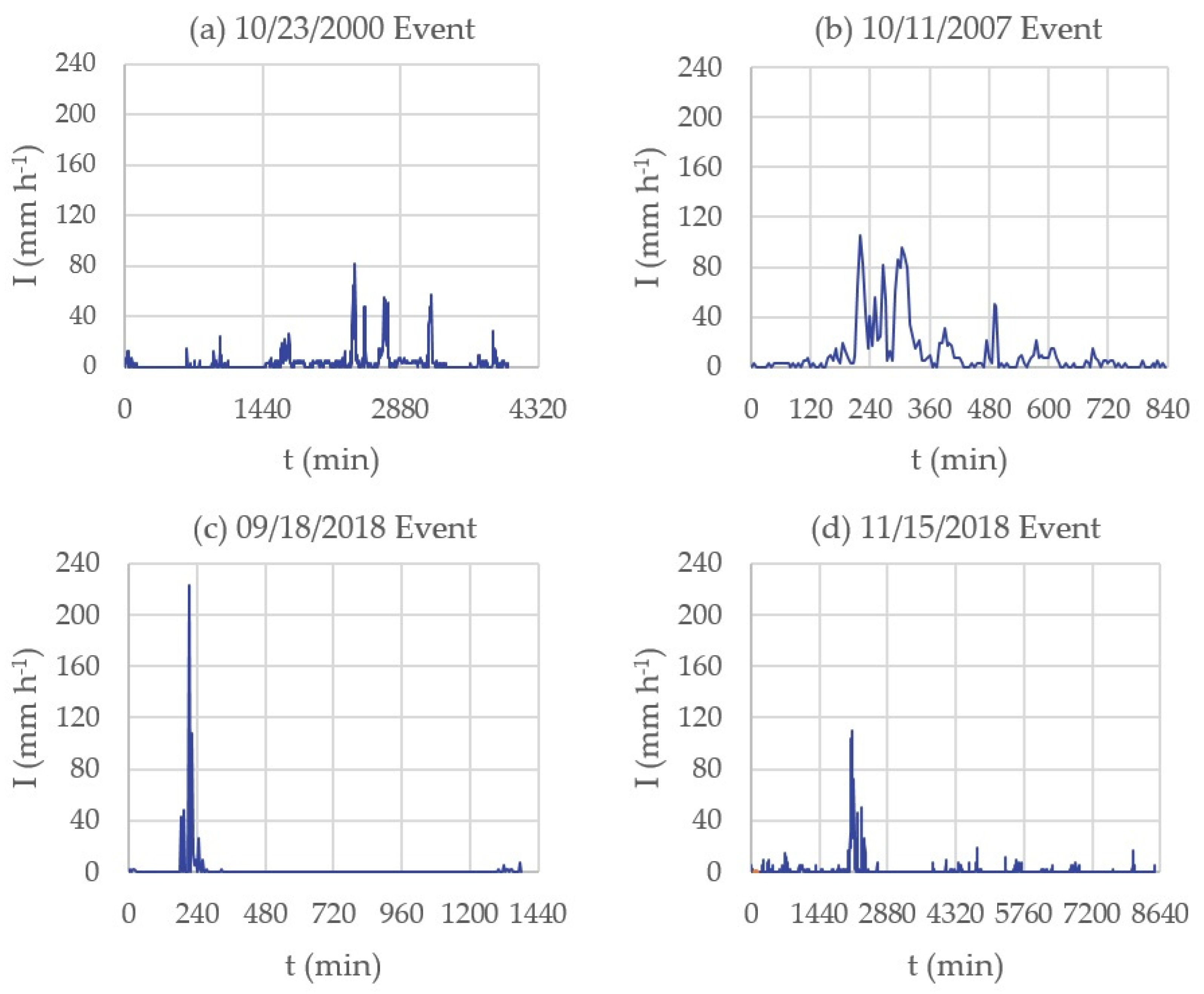
The historical time period analysed covers 30 years, ranging from 1990 until 2019. The time level of aggregation of the data series is 5 min. Following the procedure detailed in [19], a total of 70 rainstorms were identified and extracted from the original time series. All of them present one or more internal time intervals with recorded rainfall intensities over 50 mm h⁻¹. Figure 2 shows the hyetographs corresponding to some of the events taken from the sample.

Table 1. Univariate statistics obtained from the sample.

	Storm Duration D (min)	Maximum Intensity I5 (mm h−1)	Rainfall Depth V (mm)
Maximum	8530.0	223.2	220.8
Minimum	15.0	50.4	5.2
Mean	1049.3	96.9	43.8
Median	530.0	82.8	26.3
Standard deviation	1484.2	42.8	46.7
Bias	2.9	1.2	2.1
Kurtosis	10.8	0.8	3.9

shows some relevant empirical statistics obtained from the sample: the storm duration (D), the maximum intensity for a 5 min interval (I₅) and the total rainfall depth (V).

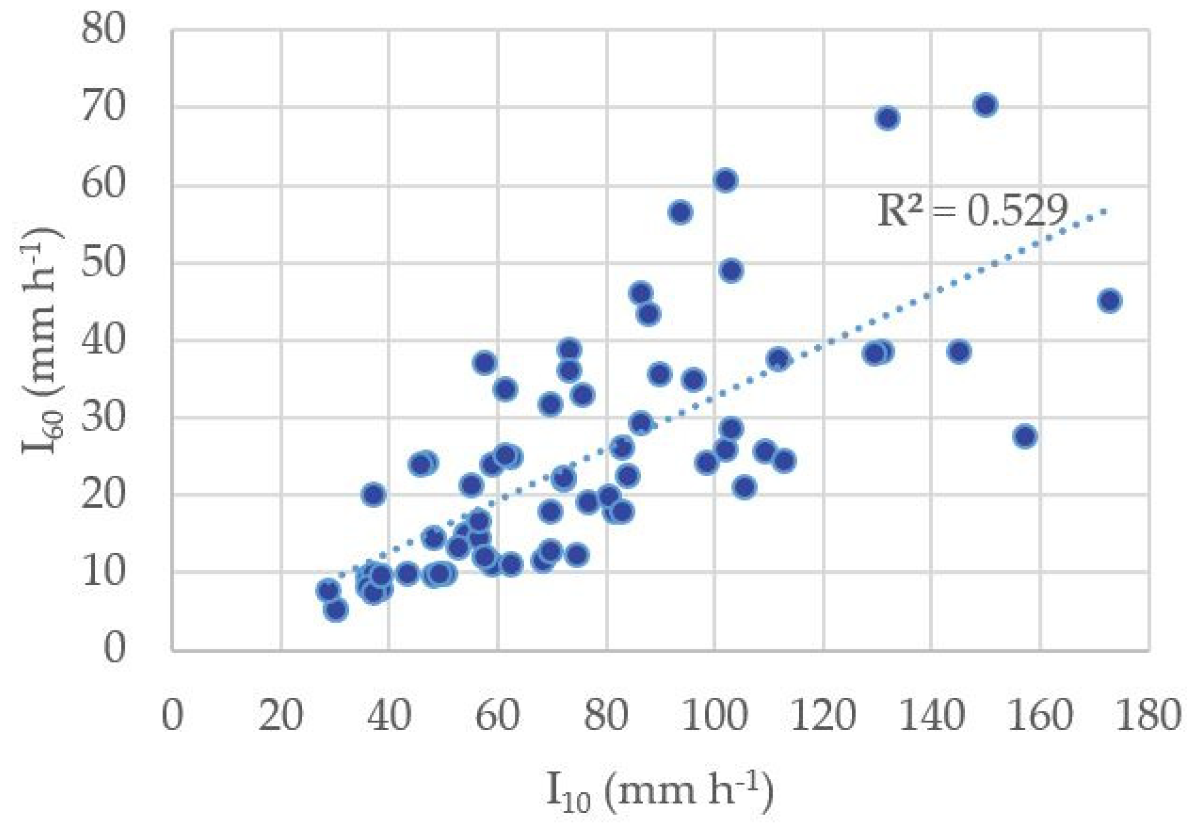
For each of the selected rainstorms, maximum rainfall intensities for durations of 10 min and 1 h were calculated. Figure 3 shows the resultant scatterplot, each point corresponding to one rainstorm of the sample. As shown in Figure 3, a significant statistical correlation exists between both variables, with an empirical determination coefficient of R² = 0.529.

The n-index [34,35] describes the temporal intra-event structure of rainfall using a dimensionless index (Equation (1)),

$$\frac{{\mathrm{I}}_{{\mathsf{\Delta }\mathrm{t}}_1}}{{\mathrm{I}}_{{\mathsf{\Delta }\mathrm{t}}_2}}\approx {\left(\frac{\mathsf{\Delta }{\mathrm{t}}_2}{\mathsf{\Delta }{\mathrm{t}}_1}\right)}^{\mathrm{n}}$$

(1)

where ${\mathrm{I}}_{{\mathsf{\Delta }\mathrm{t}}_1}$ is the average maximum intensity for a duration or time interval $\mathsf{\Delta }{\mathrm{t}}_1$; ${\mathrm{I}}_{{\mathsf{\Delta }\mathrm{t}}_2}$ is the average maximum intensity for a duration or time interval $\mathsf{\Delta }{\mathrm{t}}_2$; n is a dimensionless index (n ∈ [0; 1]). Using the above potential function, it is possible to describe the temporal distribution of any type of precipitation as a function of the n-index, regardless the total amount of cumulative precipitation.

Table 2. Storm classification according to intensity regularity vs. time. Adapted from Refs. [37,38].

n	Type of Curve	Intensity	Temporal Distribution	Interpretation of Rainfall Type
0.00–0.20	Very gentle	Practically constant	Very regular	Stationary/highly predominantly advective
0.20–0.40	Gentle	Lightly variable	Regular	Predominantly advective
0.40–0.60	Normal	Variable	Irregular	Effective
0.60–0.80	Pronounced	Moderately variable	Very irregular	Predominantly convective
0.80–1.00	Very pronounced	Strongly variable	Nearly instantaneous	Highly predominantly convective

shows the proposed five-level classification of storms based on n-index values.

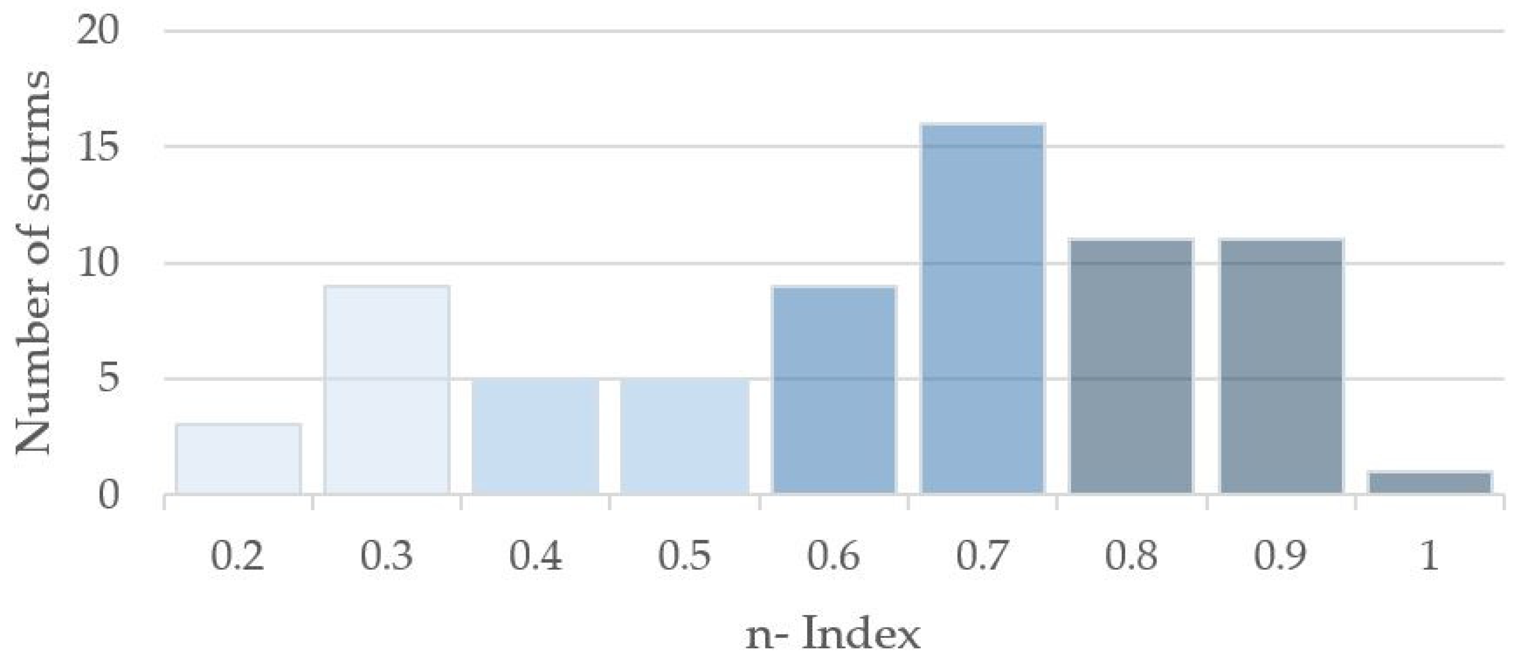
The n-index was estimated for each of the storms, using Equation (1). Figure 4 shows the empirical distribution of n-values in the sample. According to it, 68.57% of the selected events present values over 0.60, associated to dominantly convective storms according to the n-index classification (Table 2).

2.3. Return Period Assignment

Following the methodology in [19], a criterion to quantify the storm magnitude based on a principal component analysis (PCA) is used herein. The underlying idea here is to evaluate the importance of the rainstorm attending to both its maximum 10-minute rainfall intensity and the 1-hour cumulative rainfall. Therefore, we are assuming that both of them are relevant when quantifying the magnitude of the event, in terms of its potential capacity to produce drainage problems in an urban hydrology context.

The PCA yields to the definition of two new variables, X₁ and X₂, first and second principal components, respectively. The first one, X₁, is found to explain in this case 92.73% of the total variance. Accordingly, it can be reasonably considered a measurement of the storm magnitude, involving both original variables (I₁₀ and I₆₀). Introducing this new variable implies in statistical terms to handle in a single variable that contains by itself more information than any of the two original ones. On the other hand, it facilitates the return period assignment to the storm, requiring the use of a single statistical variable. Equation (2) shows the linear relationship between X₁ and I₁₀, I₆₀, resulting from the PCA.

$${\mathrm{X}}_1={0.939\mathrm{I}}_{10}+{0.343\mathrm{I}}_{60}$$

(2)

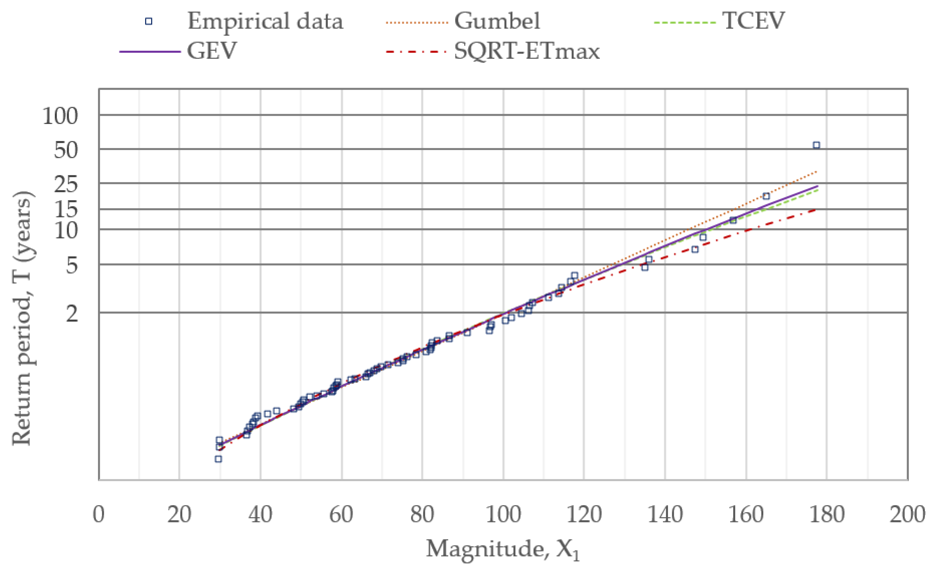
Several extreme value distributions have been explored to model variable X₁. In particular, general extreme value (GEV) [39,40], Gumbel [41], SQRT-ETmax [42] and two-component extreme value (TCEV) [43] distributions were compared. In all cases, parameters have been estimated by the method of maximum likelihood estimation (MLE).

Table 3. Estimated parameters of the fitted distribution functions.

	Cumulative Distribution Function (CDF)	Parameters
GEV [39,40]	$\mathrm{F}\left(\mathrm{x}\right)=\exp \left[-{\left(1-\frac{\mathsf{\beta }}{\mathsf{\alpha }}\left({\mathrm{x}-\mathrm{x}}_0\right)\right)}^{\frac{1}{\mathsf{\beta }}}\right]$	α	β	x0
		26.0882	−0.0480	62.324
Gumbel [41]	$\mathrm{F}\left(\mathrm{x}\right)=\exp (-\mathsf{\lambda }\exp \left(-\mathsf{\theta }\mathrm{x}\right))$	θ	λ
		0.0376	10.6652
SQRT-ET max [42]	$\mathrm{F}\left(\mathrm{x}\right)=\exp \left[-\mathsf{\kappa }\left(1+\sqrt{\mathsf{\alpha }\mathrm{x}}\right)\exp (-\sqrt{\mathsf{\alpha }\mathrm{x}})\right]$	α	κ
		0.5219	41.8091
TCEV [43]	$\mathrm{F}\left(\mathrm{x}\right)=\exp \left[{-\mathsf{\lambda }}_1\exp \left({-\mathsf{\theta }}_1\mathrm{x}\right){-\mathsf{\lambda }}_2{\exp (-\mathsf{\theta }}_2\mathrm{x})\right]$	θ1	θ2	λ1	λ2
		0.0456	0.0265	11.1031	1.8180

shows the estimated values for each of the four distribution functions considered.

There are many plotting position formulas available in the literature [44]. For the case under study herein, the Gringorten formula was chosen [45] Equation (3).

$${\mathrm{F}}_{\mathrm{j}}=\frac{\mathrm{j}-0.44}{\mathrm{N}+0.12}$$

(3)

where F_j is the estimate of the cumulative frequency of the jth term, j is the order of the observation from the smallest, and N is the number of observations. This expression provides an almost unbiased plotting position for the special case of Gumbel distribution. In practice, though, it is commonly used and suitable to assign empirical probabilities when dealing with samples of maximum values, as is the case [45,46,47,48,49].

Figure 5 shows a graphical comparison between the several theoretical distributions tested in this analysis.

The goodness of fit was assessed by means of the χ² test and the Akaike information criteria (AIC) [50].

Table 4. Goodness-of-fit test statistics.

Criterion	SQRT-ET Max	TCEV	Gumbel	GEV
χ2	0.1896	0.1709	0.1542	0.1537
AIC	686.096	686.100	686.078	685.890

shows the resulting values for each of the functions. According to them, the GEV distribution function was selected, providing best statistics for both tests. Quantiles derived from the GEV distribution function are shown in

Table 5. Estimated quantiles for X₁ derived from the GEV analysis.

T (Years)	2	5	10	15	25	50
X1 (-)	100.73	129.05	150.38	163.02	179.20	201.68

.

3. G2P Design Storm Estimation from the Rainfall Convectivity n-Index

3.1. G2P Design Storm: Analytical Definition

The G2P design storm was introduced by García-Bartual and Andrés-Doménech [19]. This design storm was specifically developed for urban hydrology applications. It comprises the definition of a theoretical storm using only two parameters within a compact analytical definition based on a two-parameter gamma function. The rainfall intensity during a storm is represented through a functional form given by Equation (4)

$$\mathrm{I}\left(\mathrm{t}\right){=\mathrm{i}}_0{\mathsf{\phi }\mathrm{t}\mathrm{e}}^{1-\mathsf{\phi }\mathrm{t}}$$

(4)

where t (min) is the time elapsed from the beginning of the rainfall event, i (t) (mm h⁻¹) is the rainfall intensity in each instant t, i₀ (mmh⁻¹) is a scale parameter representative of the instantaneous peak intensity of the rainfall event, and φ (min⁻¹) is the storm shape parameter.

The resulting design storm can be discretized in intervals of any chosen time level of aggregation. Additionally, the methodology provides an easy way to build in practice a design storm for any location in a given geographical region, based on a previous regionalization of the two parameters involved.

Among the several analytical derived properties presented in [19], we will make use herein of Equation (5), providing the maximum rainfall intensity for a given duration Δt.

$${\mathrm{I}}_{\mathsf{\Delta }\mathrm{t}}=\frac{{\mathrm{i}}_0}{\mathsf{\Delta }\mathrm{t}}\left[\left({\mathrm{t}}_{\mathrm{L}}+\frac{1}{\mathsf{\phi }}\right){\mathrm{e}}^{{1-\mathsf{\phi }\mathrm{t}}_{\mathrm{L}}}-\left({\mathrm{t}}_{\mathrm{U}}+\frac{1}{\mathsf{\phi }}\right){\mathrm{e}}^{{1-\mathsf{\phi }\mathrm{t}}_{\mathrm{U}}}\right]$$

(5)

t_L and t_U being the lower and upper limits of the central interval in the design storm (Equation (6)).

$$\left[{\mathrm{t}}_{\mathrm{L}}{;\mathrm{t}}_{\mathrm{U}}\right]=\left[\frac{\mathsf{\Delta }\mathrm{t}}{{\mathrm{e}}^{\mathsf{\phi }\mathsf{\Delta }\mathrm{t}}-1}{;\mathrm{t}}_{\mathrm{L}}+\mathsf{\Delta }\mathrm{t}\right]$$

(6)

Combining Equations (5) and (6), we obtain the following analytical expression for ${\mathrm{I}}_{\mathsf{\Delta }\mathrm{t}}$:

$${\mathrm{I}}_{\mathsf{\Delta }\mathrm{t}}=\frac{{\mathrm{i}}_0}{\mathsf{\Delta }\mathrm{t}}\mathrm{F}\left(\mathsf{\phi },\mathsf{\Delta }\mathrm{t}\right)$$

(7)

where

$$\mathrm{F}\left(\mathsf{\phi },\mathsf{\Delta }\mathrm{t}\right){=\mathrm{e}}^{{1-\mathsf{\phi }\mathrm{t}}_{\mathrm{L}}}\left[\left({\mathrm{t}}_{\mathrm{L}}+\frac{1}{\mathsf{\phi }}\right){-\mathrm{e}}^{-\mathsf{\phi }\mathsf{\Delta }\mathrm{t}}\left({\mathrm{t}}_{\mathrm{U}}+\frac{1}{\mathsf{\phi }}\right)\right]$$

(8)

3.2. Relationship between the G2P Shape Parameter and the n-Index

The n-index (Equation (1)) can be particularized for the chosen time intervals Δt₁ = 10 min and Δt₂ = 60 min.

$$\frac{{\mathrm{I}}_{10}}{{\mathrm{I}}_{60}}={\left(\frac{60}{10}\right)}^{\mathrm{n}}{=6}^{\mathrm{n}}$$

(9)

Applying Equation (7) for the specific time intervals Δt₁ = 10 min and Δt₂ = 60 min, the theoretical ratio $\frac{{\mathrm{I}}_{10}}{{\mathrm{I}}_{60}}$ is given by Equation (10).

$$\frac{{\mathrm{I}}_{10}}{{\mathrm{I}}_{60}}=\frac{60}{10}\frac{\mathrm{F}(\mathsf{\phi },10)}{\mathrm{F}(\mathsf{\phi },60)}$$

(10)

Combination of Equations (9) and (10) provide a practical relationship between the n-index and the shape parameter φ of the G2P design storm (Equation (11)).

$$\mathrm{n}=1+0.558\ln \frac{\mathrm{F}(\mathsf{\phi },10)}{\mathrm{F}(\mathsf{\phi },60)}$$

(11)

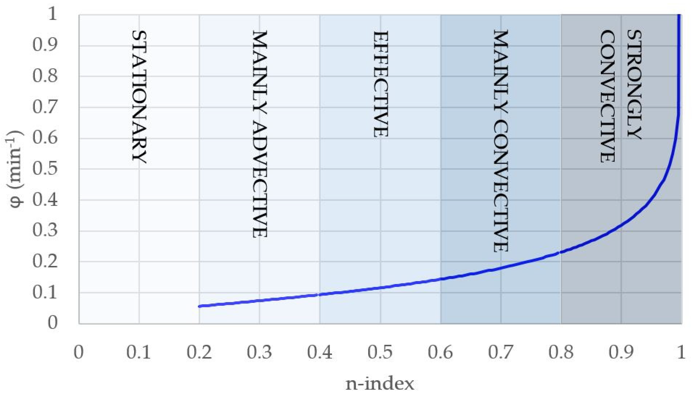
Such expression in Equation (11) is particularly useful, as it allows to link the G2P φ-parameter with the convectivity degree classification used by [37] (Table 2). In a practical context of applied urban hydrology, characteristic convectivity of rainfalls in a given geographical location can be used to assess recommendable values for the G2P design storm shape parameter, φ (min ⁻¹). Figure 6 shows the relationship between the n-index and φ, according to Equation (11). The different categories shown in Table 2 are illustrated in the graph. Higher convectivity is linked to upper values of the G2P shape parameter. For coastal Mediterranean regions in Spain, strongly affected by an extreme hydrological regimen, typical values of φ are in the range 0.08 to 0.31 for design purposes [19].

3.3. Practical Estimation of the G2P Design Storm for Urban Drainage Applications

Definition of the G2P design storm implies the estimation of parameters φ (shape parameter) and i₀ (scale parameter) in Equation (4). This estimation can be achieved in different ways, depending on the available rainfall information in a particular geographical location, from the simpler case with only IDF curves information available to a case similar to the one introduced herein (Valencia), where a detailed insight analysis of historical storms extracted from high temporal resolution series is available.

For this case study, and according to the rainfall data described in Section 2.2, there is enough information to define several possible design storms for a given return period. For illustration purposes, a return period T = 25 years will be adopted, as being the one required by the local administration for urban hydraulic infrastructure design. The steps to build a family of G2P design storms are the following.

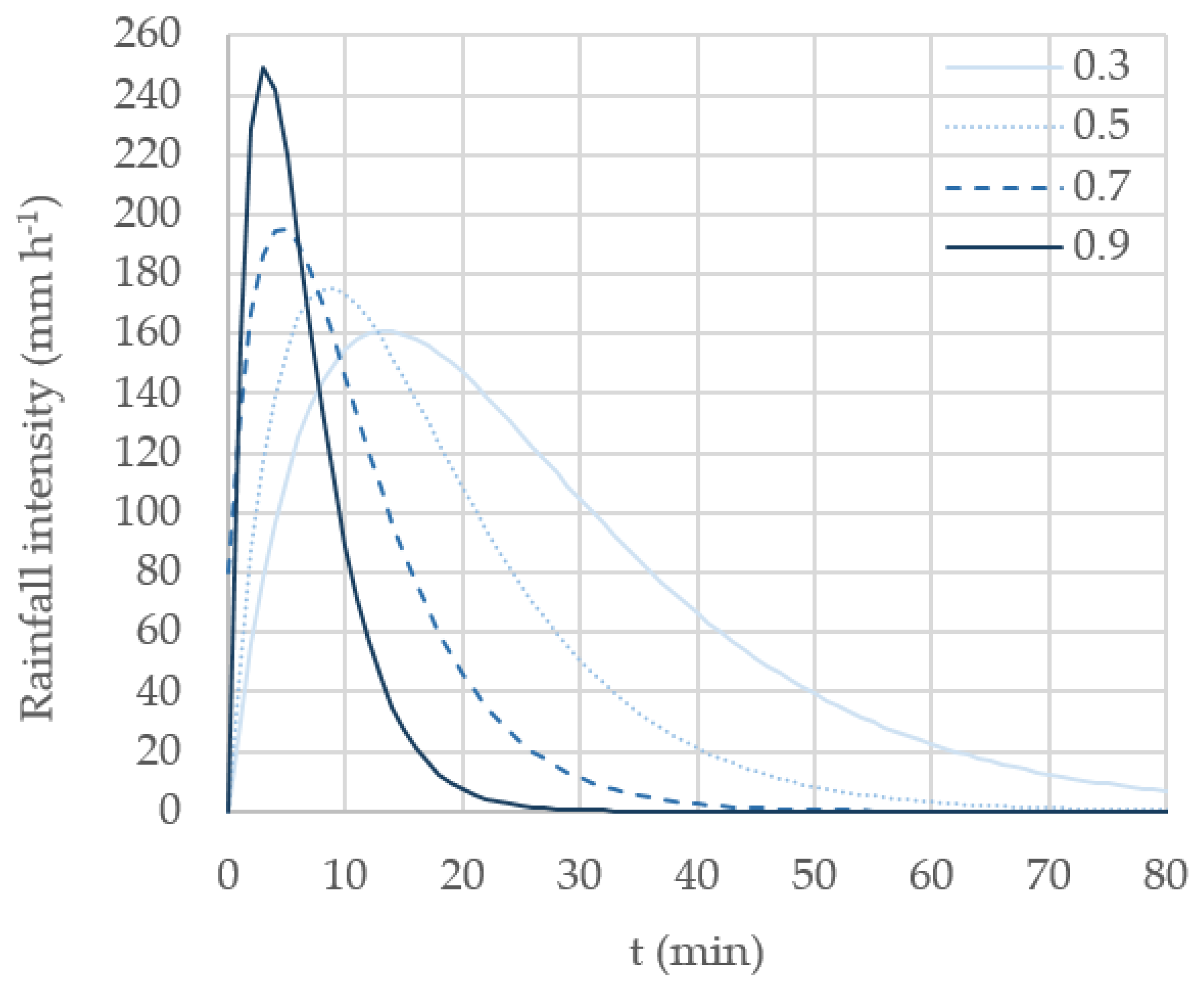
• Shape parameter, φ (min⁻¹). It derives directly from the possible convectivity quantified in through the n-index, using Equation (11). Figure 6 shows the distribution of n-index values for the particular case study analysed herein. For each of the classes assumed, a representative central n-index value is adopted, i.e., n = 0.3, 0.5, 0.7 and n = 0.9. Different probabilities of occurrence might be assigned through the empirical histogram shown in Figure 4. In any case, Equation (11) provides a unique φ value for each of the selected n-index values.

  Table 6. Shape parameter, φ, assigned for each n-index value selected.

  Storm Classification	n	φ (min−1)
  Mainly advective	0.3	0.0745
  Effective	0.5	0.1163
  Mainly convective	0.7	0.1799
  Strongly convective	0.9	0.3189

  shows the G2P shape parameter assigned to each of the representative n-index values.
• Scale parameter, i₀ (mm h⁻¹). It basically depends on the return period. For T = 25 years, an X₁ quantile is estimated (Table 5): X₁ = 179.20. Then, solving Equations (2) and (9), we obtain I₁₀ = 157.27 mm h⁻¹ and I₆₀ = 91.88 mm h⁻¹. Finally, i₀ is obtained from Equation (7), using either Δt = 10 min or Δt = 60 min. The resultant estimated values for the scale parameters are: i₀ = 160.90 mm h⁻¹ (for n = 0.3); i₀ = 175.33 mm h⁻¹ (for n = 0.5); i₀ = 195.72 mm h⁻¹ (for n = 0.7); i₀ = 249.55 mm h⁻¹ (for n = 0.9).

Figure 7 shows the four design storms defined in this way, all of them associated to a return period of T = 25 years, for the presented case study in Valencia. As explained before, each of these theoretical hyetographs are defined exclusively in terms of two parameters. On the other hand, they can be conveniently discretized as needed using a given time level of aggregation [19].

For a given practical case where only IDF rainfall information is available, a shortcut in the procedure is to be applied. Readings of I₁₀ and I₆₀ values from the ID curve (for T = 25 years, to continue with the same example) are needed to obtain the n-index value (Equation (9)). Then, φ (shape parameter) is obtained after Equation (11), while scale parameter i₀ is again calculated from Equation (7).

For the case of Valencia city in Spain, the ID curve for T = 25 years is given by the local authorities [51] I₁₀ = 133.3 (mm h⁻¹), I₆₀ = 70.1 (mm h⁻¹) for the adopted return period. Thus, $\frac{{\mathrm{I}}_{10}}{{\mathrm{I}}_{60}}$= 1.9017, and n= 0.359. From Equation (11), φ = 0.0856 min⁻¹, and finally, i₀ = 137.3 mm h⁻¹, from Equation (7).

Proceeding in such way, IDF curves might be easily translated into analytical forms of design storms, setting the basis for regionalization of design storms for a given geographical area. This strategy obviously requires at least availability of IDF curves information over the studied area.

4. Conclusions

Many real-world applications dealing with urban drainage systems are performed using as main inputs fine-resolution historical rainfall records or even synthetic series generated through stochastic models. However, the old concept of design storms, as well as the classical intensity–duration–frequency curves, still have a significant interest for some engineering applications, especially in geographical points with a lack of high-resolution rainfall data. In such case, technical recommendations can assess design criteria on a regional basis. The G2P storm definition involves only two parameters, and thus, it is particularly suitable for this kind of approaches. Some analytical features of the G2P design storm are reviewed herein, and a useful relationship is proposed, allowing the estimation of the shape of the storm from the n-index rainfall convectivity index.

A practical application for the case of Valencia (Spain) is presented, using as input high-resolution time series of rainfall intensity. This kind of data allows us to perform a deep analysis, yielding to the estimation of the design storm directly from the observed internal features of the rainfall intensity process at the finest scale. On the other hand, a direct, easy-to-apply procedure is introduced, deducing the design storm directly from the intensity–duration–frequency curves. The proposed methodology makes use of the analytical relationship with the n-index.

This versatility of the G2P design storm makes it particularly useful in the context of practical urban hydrology applications at a regional scale. In fact, many studies estimating the impacts of global climate change present their results on a regional basis, referring results to expected spatial and temporal variations of given climatic or hydrological variables [52,53,54,55,56,57]. Such variables include precipitation, streamflow and temperature, among others. Geostatistical analysis and other popular interpolation techniques are commonly used to provide useful outputs for water resources applications. Such a concept could be extended to rainfall hypotheses as an input for urban drainage applications, through the G2P design storm.

References

- Pulhin, J.M.; Inoue, M.; Shaw, R.; Pangilinan, M.J.Q.; Catudio, M.L.R.O. Climate Change and Disaster Risks in an Unsecured World. In Climate Change, Disaster Risks, and Human Security; Pulhin, J.M., Inoue, M., Shaw, R., Eds.; Springer: Singapore, 2021; pp. 1–19. [Google Scholar]
- Seneviratne, S.I.; Nicholls, N.; Easterling, D.; Goodess, C.M.; Kanae, S.; Kossin, J.; Luo, Y.; Marengo, J.; McInnes, K.; Rahimi, M. Changes in climate extremes and their impacts on the natural physical environment. In Managing the Risks of Extreme Events and Disasters to Advance Climate Change Adaptation; Field, C.B., Barros, V., Stocker, T.F., Qin, D., Dokken, D.J., Ebi, K.L., Mastrandrea, M.D., Mach, K.J., Plattner, G.-K., Allen, S.K., et al., Eds.; A Special Report of Working Groups I and II of the Intergovernmental Panel on Climate Change (IPCC); Cambridge University Press: Cambridge, UK; New York, NY, USA, 2012; pp. 109–230. [Google Scholar]
- Westra, S.; Fowler, H.J.; Evans, J.P.; Alexander, L.V.; Berg, P.; Johnson, F.; Kendon, E.J.; Lenderink, G.; Roberts, N.M. Fu-ture Changes to the Intensity and Frequency of Short-Duration Extreme Rainfall. Rev. Geophys. 2014, 52, 522–555. [Google Scholar] [CrossRef]
- Myhre, G.; Alterskjær, K.; Stjern, C.W.; Hodnebrog, Ø.; Marelle, L.; Samset, B.H.; Sillmann, J.; Schaller, N.; Fischer, E.; Schulz, M.; et al. Frequency of extreme precipitation increases extensively with event rareness under global warming. Sci. Rep. 2019, 9, 1–10. [Google Scholar] [CrossRef] [Green Version]
- Hannaford, J.; Marsh, T.J. High-flow and flood trends in a network of undisturbed catchments in the UK. Int. J. Clim. 2008, 28, 1325–1338. [Google Scholar] [CrossRef] [Green Version]
- Volosciuk, C.; Maraun, D.; Semenov, V.A.; Tilinina, N.; Gulev, S.K.; Latif, M. Rising Mediterranean Sea Surface Temperatures Amplify Extreme Summer Precipitation in Central Europe. Sci. Rep. 2016, 6, 32450. [Google Scholar] [CrossRef]
- Forestieri, A.; Caracciolo, D.; Arnone, E.; Noto, L. Derivation of Rainfall Thresholds for Flash Flood Warning in a Sicilian Basin Using a Hydrological Model. Procedia Eng. 2016, 154, 818–825. [Google Scholar] [CrossRef] [Green Version]
- Cipolla, G.; Francipane, A.; Noto, L.V. Classification of Extreme Rainfall for a Mediterranean Region by Means of Atmos-pheric Circulation Patterns and Reanalysis Data. Water Resour. Manag. 2020, 34, 3219–3235. [Google Scholar] [CrossRef]
- Kuichling, E. The Relation between the Rainfall and the Discharge of Sewers in Populous Districts. Trans. Am. Soc. Civ. Eng. 1889, 20, 1–56. [Google Scholar] [CrossRef]
- Yen, B.C.; Chow, V.T. Closure to “Design Hyetographs for Small Drainage Structures”. J. Hydraul. Div. 1981, 107, 945–946. [Google Scholar] [CrossRef]
- Sifalda, V. Entwicklung eines Berechnungsregens für die Bemessung von Kanalnetzen. Gwf-Wasser/Abwasser 1973, 114, 435–440. (In German) [Google Scholar]
- Desbordes, M. Urban Runoff and Design Storm Modelling. In Proceedings of the International Conference on Urban Storm Drainage, Southampton, UK, 11–14 April 1978; Pentech Press: London, UK, 1978; pp. 353–361. [Google Scholar]
- Watt, W.E.; Chow, K.C.A.; Hogg, W.D.; Lathem, K.W. A 1-h urban design storm for Canada. Can. J. Civ. Eng. 1986, 13, 293–300. [Google Scholar] [CrossRef]
- Keifer, C.J.; Chu, H.H. Synthetic Storm Pattern for Drainage Design. J. Hydraul. Div. 1957, 83, 1332. [Google Scholar] [CrossRef]
- Te Chow, V.; Maidment, D.R.; Mays, L.W. Applied Hydrology; McGraw-Hill: New York, NY, USA, 1988. [Google Scholar]
- Terstriep, M.L.; Stall, J.B. The Illinois Urban Drainage Area Simulator, ILLUDAS; Bulletin 58; Illinois State Water Survey: Urbana, IL, USA, 1974. [Google Scholar]
- Cronshey, R. Urban Hydrology for Small Watersheds; US Department of Agriculture, Soil Conservation Service, Engineering Division: Washington, DC, USA, 1986.
- Pilgrim, D.H.; Cordery, I. Rainfall Temporal Patterns for Design Floods. J. Hydraul. Div. 1975, 101, 81–95. [Google Scholar] [CrossRef]
- García-Bartual, R.; Andrés-Doménech, I. A two-parameter design storm for Mediterranean convective rainfall. Hydrol. Earth Syst. Sci. 2017, 21, 2377–2387. [Google Scholar] [CrossRef] [Green Version]
- Balbastre-Soldevila, R.; García-Bartual, R.; Andrés-Doménech, I. A Comparison of Design Storms for Urban Drainage System Applications. Water 2019, 11, 757. [Google Scholar] [CrossRef] [Green Version]
- Gutierrez-Lopez, A.; Jimenez-Hernandez, S.B.; Escalante Sandoval, C. Physical Parameterization of IDF Curves Based on Short-Duration Storms. Water 2019, 11, 1813. [Google Scholar] [CrossRef] [Green Version]
- Schertzer, D.; Lovejoy, S. Physical Modeling and Analysis of Rain and Clouds by Anisotropic Scaling Mutiplicative Processes. J. Geophys. Res. 1987, 92, 9693–9714. [Google Scholar] [CrossRef]
- Gupta, V.K.; Waymire, E.C. A Statistical Analysis of Mesoscale Rainfall as a Random Cascade. J. Appl. Meteorol. 1993, 32, 251–267. [Google Scholar] [CrossRef]
- Koutsoyiannis, D.; Onof, C.; Wheater, H.S. Multivariate rainfall disaggregation at a fine timescale. Water Resour. Res. 2003, 39. [Google Scholar] [CrossRef]
- Westra, S.; Mehrotra, R.; Sharma, A.; Srikanthan, R. Continuous rainfall simulation: 1. A regionalized subdaily disaggregation approach. Water Resour. Res. 2012, 48, 1–16. [Google Scholar] [CrossRef] [Green Version]
- Müller-Thomy, H. Temporal rainfall disaggregation using a micro-canonical cascade model: Possibilities to improve the autocorrelation. Hydrol. Earth Syst. Sci. 2020, 24, 169–188. [Google Scholar] [CrossRef] [Green Version]
- Vašková, I. Cálculo de Las Curvas Intensidad-Duración-Frecuencia Mediante La Incorporación de Las Propiedades de Escala y de Dependencia Temporales. PhD Thesis, Universitat Politècnica de València, Valencia, Spain, 2001. (In Spanish). [Google Scholar]
- García-Marín, A.P. Análisis Multifractal de Series de Datos Pluviométricos En Andalucía. PhD Thesis, Universidad de Cór-doba, Córdoba, Spain, 2007. [Google Scholar]
- Martin-Vide, J. Spatial distribution of a daily precipitation concentration index in peninsular Spain. Int. J. Clim. 2004, 24, 959–971. [Google Scholar] [CrossRef]
- Maraun, D.; Osborn, T.J.; Gillett, N.P. United Kingdom daily precipitation intensity: Improved early data, error estimates and an update from 2000 to 2006. Int. J. Clim. 2008, 28, 833–842. [Google Scholar] [CrossRef]
- Llasat, M.C. An Objective Classification of Rainfall Events on the Basis of Their Convective Features: Application to Rainfall Intensity in the Northeast of Spain. Int. J. Climatol. 2001, 21, 1385–1400. [Google Scholar] [CrossRef]
- Casas, M.C.; Codina, B.; Lorente, J. A methodology to classify extreme rainfall events in the western mediterranean area. Theor. Appl. Clim. 2004, 77, 139–150. [Google Scholar] [CrossRef]
- Moncho, R. Análisis de La Intensidad de Precipitación. Método de La Intensidad Contigua. RAM3. January 2008. Available online: https://afly.co/slm5 (accessed on 10 June 2021). (In Spanish).
- Monjo, R. Measure of rainfall time structure using the dimensionless n-index. Clim. Res. 2016, 67, 71–86. [Google Scholar] [CrossRef] [Green Version]
- Monjo, R.; Martin-Vide, J. Daily precipitation concentration around the world according to several indices. Int. J. Clim. 2016, 36, 3828–3838. [Google Scholar] [CrossRef]
- Peel, M.C.; Finlayson, B.L.; McMahon, T.A. Updated World Map of the Köppen-Geiger Climate Classification. Hydrol. Earth Syst. Sci. 2007, 11, 1633–1644. [Google Scholar] [CrossRef] [Green Version]
- Moncho, R.; Belda, F.; Caselles, V. Climatic Study of the Exponent “n” in IDF Curves: Application for the Iberian Peninsula. Thethys 2009, 6, 3–14. [Google Scholar] [CrossRef] [Green Version]
- Monjo, R. El Índice n de la Precipitación Intensa. Available online: https://bit.ly/3veM9bL (accessed on 10 June 2021). (In Spanish).
- Jenkinson, A.F. The frequency distribution of the annual maximum (or minimum) values of meteorological elements. Q. J. R. Meteorol. Soc. 1955, 81, 158–171. [Google Scholar] [CrossRef]
- Jenkinson, A.F. Estimation of Maximum Floods. World Meteorol. Organ. Tech. Note 1969, 98, 183–257. [Google Scholar]
- Gumbel, E.J. Statistics of Extremes; Columbia University Press: New York, NY, USA, 1958. [Google Scholar]
- Etoh, T.; Murota, A.; Nakanishi, M. SQRT-Exponential Type Distribution of Maximum. In Proceedings of the International Symposium on Flood Frequency and Risk Analyses, Baton Rouge, LA, USA, 14–17 May 1986; Springer: Dordrecht, The Netherlands, 1987; pp. 253–264. [Google Scholar]
- Rossi, F.; Fiorentino, M.; Versace, P. Two-Component Extreme Value Distribution for Flood Frequency Analysis. Water Resour. Res. 1984, 20, 847–856. [Google Scholar] [CrossRef]
- Yah, A.S.; Nor, N.M.; Rohashikin, N.; Ramli, N.A.; Ahmad, F.; Ul-Saufie, A.Z. Determination of the Probability Plotting Position for Type I Extreme Value Distribution. J. Appl. Sci. 2012, 12, 1501–1506. [Google Scholar] [CrossRef] [Green Version]
- Gringorten, I.I. A plotting rule for extreme probability paper. J. Geophys. Res. 1963, 68, 813–814. [Google Scholar] [CrossRef]
- Cunnane, C. Unbiased plotting positions—A review. J. Hydrol. 1978, 37, 205–222. [Google Scholar] [CrossRef]
- Stedinger, J.R.; Vogel, R.M.; Foufoula-Georgiou, E. Frequency analysis of extreme events. In Handbook of Hydrology; Maidment, D.A., Ed.; McGraw-Hill: New York, NY, USA, 1993; Chapter 18. [Google Scholar]
- Guo, S. A discussion on unbiased plotting positions for the general extreme value distribution. J. Hydrol. 1990, 121, 33–44. [Google Scholar] [CrossRef]
- Shabri, A.; Ani, F.N. A Comparison of Plotting Formulas for the Pearson Type III Distribution. J. Teknol. 2002, 36, 61–74. [Google Scholar] [CrossRef] [Green Version]
- Akaike, H. Information Theory and an Extension of the Maximum Likelihood Principle. In Selected Papers of Hirotugu Akaike; Parzen, E., Tanabe, K., Kitagawa, G., Eds.; Springer: New York, NY, USA, 1998; pp. 199–213. [Google Scholar]
- Ajuntament de València. Normativa Para Obras de Saneamiento y Drenaje Urbano de la Ciudad de Valencia. Ciclo Integral del Agua. 2016. Available online: https://www.ciclointegraldelagua.com/castellano/normativa-documentacion.php (accessed on 13 June 2021).
- Hailegeorgis, T.; Thorolfsson, S.T.; Alfredsen, K. Regional frequency analysis of extreme precipitation with consideration of uncertainties to update IDF curves for the city of Trondheim. J. Hydrol. 2013, 498, 305–318. [Google Scholar] [CrossRef] [Green Version]
- Bharath, R.; Srinivas, V.V. Regionalization of extreme rainfall in India. Int. J. Clim. 2015, 35, 1142–1156. [Google Scholar] [CrossRef]
- Darwish, M.M.; Fowler, H.J.; Blenkinsop, S.; Tye, M.R. A Regional Frequency Analysis of UK Sub-Daily Extreme Precipita-tion and Assessment of Their Seasonality. Int. J. Climatol. 2018, 38, 4758–4776. [Google Scholar] [CrossRef]
- Chavan, S.R.; Srinivas, V.V. Regionalization based envelope curves for PMP estimation by Hershfield method. Int. J. Clim. 2016, 37, 3767–3779. [Google Scholar] [CrossRef]
- Zhang, Z.; Stadnyk, T.A. Investigation of Attributes for Identifying Homogeneous Flood Regions for Regional Flood Fre-quency Analysis in Canada. Water 2020, 12, 2570. [Google Scholar] [CrossRef]
- Yang, Z. The unscented Kalman filter (UKF)-based algorithm for regional frequency analysis of extreme rainfall events in a nonstationary environment. J. Hydrol. 2021, 593, 125842. [Google Scholar] [CrossRef]
Figure 1.
Location of the rain gauge station in Valencia. Images taken from Institut Cartogràfic Valencià, Generalitat Valenciana (https://visor.gva.es/visor/, accessed on 3 July 2021) and Google Earth.
Figure 2.
Representative hyetographs of some events from the sample. (a) Hyetograph of the 10/23/2000 event; (b) hyetograph of the 10/11/2007 event; (c) hyetograph of the 09/18/2018 event; (d) hyetograph of the 11/15/2018 event.
Figure 3.
Observed values [I10-min; I60-min].
Figure 4.
n-index frequency histogram.
Figure 5.
Theoretical distribution functions describing variable X1.
Figure 6.
Relationship between the n-index and φ.
Figure 7.
G2P design storms for T = 25 years in Valencia (Spain).