
Investigating Groundwater Condition and Seawater Intrusion Status in Coastal Aquifer Systems of Eastern India


1
AgFE Department, IIT Kharagpur, Kharagpur 721302, India
2
WRD&M Department, IIT Roorkee, Roorkee 247667, India
*
Author to whom correspondence should be addressed.
Water 2021, 13(14), 1952; https://doi.org/10.3390/w13141952
Submission received: 21 May 2021
/
Revised: 28 June 2021
/
Accepted: 9 July 2021
/
Published: 16 July 2021
(This article belongs to the Special Issue Groundwater Flow Modeling in Coastal Aquifers)
Abstract
:Providing sustainable water supply for domestic needs and irrigated agriculture is one of the most significant challenges for the current century. This challenge is more daunting in coastal regions. Groundwater plays a pivotal role in addressing this challenge and hence, it is under growing stress in several parts of the world. To address this challenge, a proper understanding of groundwater characteristics in an area is essential. In this study, spatio-temporal analyses of pre-monsoon and post-monsoon groundwater levels of two coastal aquifer systems (upper leaky confined and underlying confined) were carried out in Purba Medinipur District, West Bengal, India. Trend analysis of seasonal groundwater levels of the two aquifers systems was also performed using Mann-Kendall test, Linear Regression test, and Innovative Trend test. Finally, the status of seawater intrusion in the two aquifers was evaluated using available groundwater-quality data of Chloride (Cl−) and Total Dissolved Solids (TDS). Considerable spatial and temporal variability was found in the seasonal groundwater levels of the two aquifers. Further, decreasing trends were spotted in the pre-monsoon and post-monsoon groundwater-level time series of the leaky confined and confined aquifers, except pre-monsoon groundwater levels in Contai-I and Deshpran blocks, and the post-monsoon groundwater level in Ramnagar-I block for the leaky confined aquifer. The leaky confined aquifer in Contai-I, Contai-III, and Deshpran blocks and the confined aquifer in Nandigram-I and Nandigram-II blocks are vulnerable to seawater intrusion. There is an urgent need for the real-time monitoring of groundwater levels and groundwater quality in both the aquifer systems, which can ensure efficient management of coastal groundwater reserves.
1. Introduction
Water is a vital substance on earth and forms the principal constituent of all living things. Therefore, it is called the lifeblood of the biosphere. The unabated population growth and implacable rise of water demand in different sectors have huge repercussions for a growing freshwater scarcity in several parts of the world, including India. Providing sustainable water for domestic use and irrigated agriculture is one of the big challenges for the 21st century. To address this challenge, efficient planning and management of water resources are of utmost importance. Groundwater is a renewable but finite resource. Generally, it is preferred for drinking water supply because of its good quality, pleasant taste, and from a safety point of view. Due to rapid population growth, water resources potential is decreasing day by day in general, and groundwater resources potential in particular. Furthermore, mismanagement of water resources and climate change create an imbalance between water supply and demand. For proper planning and management of groundwater, assessment of groundwater is very important. Nowadays, the management of coastal aquifer systems is becoming essential due to dramatic climate change. Unfortunately, groundwater management has been neglected in coastal areas, though coastal regions provide one-third of the world’s ecosystem services and natural capital [1]. Anthropogenic activities such as excessive pumping of coastal aquifers and increased impervious surfaces in urbanized areas are the major causes of saltwater intrusion. Moreover, the increasing sea level due to climate change could aggravate this problem. Human water use is a key driver in the hydrology of coastal aquifers, but water management in the coastal areas is misguided [2].
For efficient planning of water resources, statistical analyses of hydrological time series play a vital role by identifying and describing quantitatively each of the hydrological processes [3] and forecasting future values of the time series variable. The trend is one of the essential characteristics of hydrological time series, and it exists in a dataset if there is a significant correlation between observation and time. Different parametric and non-parametric methods have been used for detecting monotonic trends. However, efficient management of water resources requires both monotonic trends as well as separate trends for low, medium, and high values of the concerned variable. Such an approach helps to find drought and flood occurrences in their increasing or decreasing frequencies [4]. A novel method has been proposed by Sen (2012) [4], which is capable of determining monotonic trends as well as trends for low, medium, and high values. In the past, many studies have been focused on the detection of trends in rainfall [5,6,7,8,9,10,11,12,13,14]. The application of a set of statistical tests for the same objective in a time series analysis increases the chance of rejecting a true null hypothesis [5]. Therefore, it is important to analyze the results by considering more than two statistical tests while taking decision on rejecting the null hypothesis.
India, with a vast coastline in order of about 7500 km, has a network of major and minor delta systems and estuaries all along the coastal regions [15]. Coastal aquifers serve as major freshwater reservoirs in the coastal areas. Due to rapid population growth, stresses on coastal aquifers are increasing day by day. Nowadays, the management of coastal aquifer systems is becoming more important due to global climate change. Serious problems of saltwater intrusion exist in many coastal regions of the country including West Bengal, Odisha, Andhra Pradesh, and Tamil Nadu. In India, seawater intrusion is observed along the coastal areas of Gujarat and Tamil Nadu (http://cgwb.gov.in/documents/papers/INCID.html, accessed on 15 April 2016). A better understanding of the patterns of movement and mixing of freshwater and seawater, as well as the factors influencing these processes, is necessary to manage coastal groundwater resources efficiently.
Bhosale and Kumar (2002) [16] used SUTRA software package for the simulation of seawater intrusion in Ernakulam coast, Kerala (India) and found that the most sensitive zone for seawater intrusion laid between 400 and 2000 m from the high tide line in Ernakulam coast. Elango and Sivakumar (2008) [17] carried out a modeling study using MODFLOW on seawater intrusion in a coastal aquifer of Chennai (India) and the model showed that the total abstraction from this aquifer should be restricted to 4.25 MGD to prevent seawater intrusion. Datta et al. (2009) [18] used FEMWATER for modeling and control of seawater intrusion in a coastal aquifer in two Blocks of Nellore District, Andhra Pradesh (India). Ganesan and Thayumanavan (2009) [19] identified management strategies by the simulation of groundwater flow and solute transport in the seawater intruded coastal aquifer system of Chennai (India) using MODFLOW and MT3D. Simulation-optimization modelling studies were carried out by Sindhu et al. (2012) [20], Lathashri and Mahesha (2015) [21], and Mohan and Pramada (2015) [22] in Trivandrum, Kerala (India), sea-coast of Karnataka, and southern Chennai respectively.
In Eastern India, Rejani et al. (2007) [23] carried out simulation-optimization modelling in Balasore coastal basin, Odisha and established the most promising management strategy of reducing pumpage from the second aquifer by 50% and an increase in pumpage up to 150% from the first and second aquifer. Goswami (1968) [24] applied a geochemical approach and Shivanna et al. (1993) [25] employed environmental isotopes D, 18O, 34S, 3H, and 14C to examine seawater salinity in the coastal part of Purba Medinipur District, West Bengal. Bhattacharya and Basack (2012) [26] found out the extent of seawater intrusion by analyzing EC, Chloride, and TDS concentration of groundwater in coastal areas of Contai-Digha, West Bengal.
The literature review reveals that only a couple of preliminary geochemical investigations have been conducted in the coastal portion of West Bengal. No comprehensive scientific studies on seawater intrusion have been conducted to date in general and in West Bengal in particular. West Bengal has its own share of water problems in India. The erratic nature of the southwest monsoon has rendered surface water supply unreliable and inadequate, which in turn has compelled the people to depend more and more on groundwater for meeting the growing water demands of different sectors. Therefore, there is an urgent need for integrated management of water resources in this state using modern tools/techniques to ensure their long-term sustainability. Keeping this in mind, the present study has been undertaken with an overall objective to investigate groundwater conditions and evaluate seawater intrusion status in the coastal aquifer systems of Purba Medinipur district, West Bengal.
2. Overview of Study Area
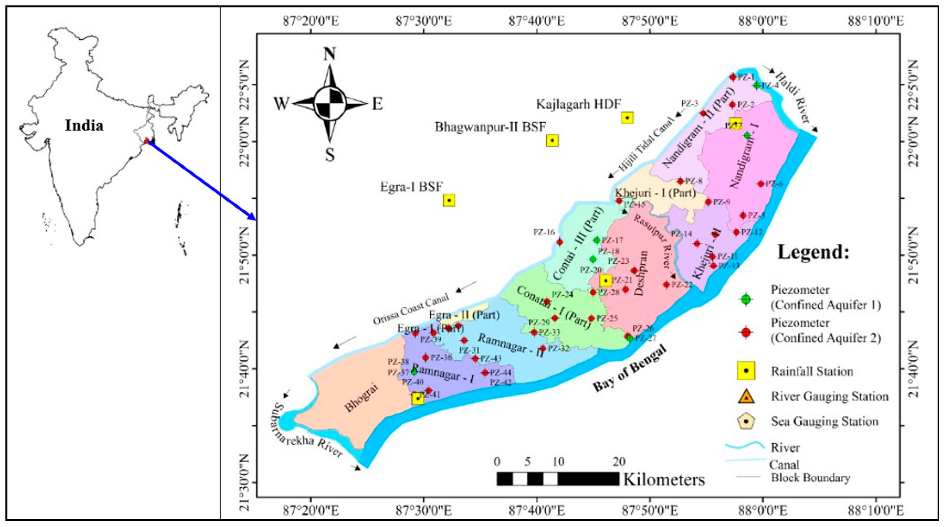
The study area selected for this study lies in the coastal area of Purba Medinipur District (West Bengal) and coastal part of Bhograi Block, Balasore District (Odisha) in India (Figure 1). It is located in the lower deltaic part of the Ganga basin and lies between latitude 21°34′41″ N and 22°00′45″ N and longitude 87°18′32″ E and 88°03′22″ E.
It covers an area of about 1398.7 km2 bounded by Haldi River in the north, Hugli River outfall in the northeast, the Bay of Bengal in the southeast, Subarnarekha River in the south, Orissa Coast Canal (OCC) in the south-west and Hugli Tidal Canal (HTC) second range in the northwest (Figure 1). The area is characterized by gently sloping flat alluvial terrain, which gradually merges to the deltaic plain towards the south. The average annual rainfall in the area is 1700 mm, out of which 73% occurs during the monsoon season lasting from June to September. The study area has a humid subtropical type of climate with maximum and minimum temperatures of 39 °C in summer and 12 °C in winter, respectively. The study area is underlain by unconsolidated alluvial sediments of quaternary age, and is overlain by linear continuous beach ridges (sand dunes) along the coastline around Digha‒Ramnagar‒Contai deposited by the wave action of the sea. The quaternary sediments are underlain by tertiary sediments of the Mio-Pliocene age (http://cgwb.gov.in/District_Profile/WestBangal/Purba%20Medinipur.pdf, accessed on 10 May 2016).
The hydrogeological investigation reveals that groundwater occurs in the Leaky Confined Aquifer (~20 to 120 m below the ground level) and Confined Aquifer (~140 to 300 m below the ground level) in this coastal area. The piezometric level in leaky confined aquifer varies 5–16 m below ground level (bgl) and 2–12 m bgl during pre-monsoon and post-monsoon season (2013), respectively. The piezometric level in confined aquifer varies 7–26 m bgl and 4–15 m bgl during pre-monsoon and post-monsoon season (2013), respectively. The piezometric-level in both the aquifers in northeastern part of the study area fluctuate below mean sea level (MSL) during pre-monsoon and post-monsoon season (2001–2015). However, the piezometric-levels in both aquifers fluctuate below MSL during pre-monsoon, and close or above MSL during post-monsoon season in the southwestern part. Groundwater flows from north-west to south-east with a hydraulic gradient varying from 1:5 to 1:6.
3. Materials and Methods
3.1. Data Used
The monthly total rainfall (1976–2015), pre-monsoon and post-monsoon average groundwater level (2001–2015) and groundwater quality (2011–2014), groundwater irrigation (2006–2007 and 2013–2014), and lithological data required for the study were collected from various state and central government organizations. The collected hydrological and meteorological data were processed in block-level and analyzed in time series using different statistical methods. Moreover, the mapping and spatial distribution of hydrological data were done on the ArcGIS platform.
3.2. Detection of Trend in Groundwater Level Time Series
In the present study, powerful statistical tests, namely the ‘Linear Regression test’, ‘Mann-Kendall test’ and ‘Innovative Trend test’ proposed by Sen (2012) [4] were used to find trends in the pre-monsoon and post-monsoon groundwater-level time series (2001–2015) of the leaky confined and confined aquifers in the study area for the available data. To carry out trend analysis, spreadsheet programs were developed using MS Excel software. Brief descriptions of these tests are given below.
3.2.1. Linear Regression Test
The least-square linear regression test is a parametric test. Before the application of this test, a normality check should be done as hydrologic and climatic data are skewed most of the time. This test used to describe the presence of linear trends in time series [27]. The test statistic (t) is defined as
where m is the estimated slope of the regression line between the observed value and time and Sm stands for the standard error of the estimated slope. The test statistic (t) follows a student’s t‒distribution with n − 2 degree of freedom, where n is the number of samples. The null hypothesis of slope zero will be rejected when the test statistic (t) value is greater than the critical value tα/2 with α significance level.
3.2.2. Mann‒Kendall Test
The Mann‒Kendall test is a non-parametric test for exploring trends in a time series without specifying the type of trend (i.e., linear or non-linear). This test has been found to be an excellent tool for trend detection [28]. Using Mann-Kendall’s test, it is possible to find the existence of a rising or falling trend, but it is hard to quantify its magnitude. The Mann-Kendall test statistic (S) is calculated as:
where, n is the number of data points, xi and xj are the data values in time series i and j (j > i), respectively, and sgn (xj − xi) is the sign function defined as:
Moreover, for n > 10, the standard normal test statistic ZS is computed as:
where,
In Equations (4) and (5), p = 1 for S < 0 and p = −1 for S > 0, k is the number of tied groups (a set of sample data having the same value), and ti is the numbers of data in the ith tied group. The value of the test-statistic ZS is considered as zero for S = 0. Positive values of ZS indicate rising trends while negative ZS values show falling trends. If the computed absolute value of ZS is greater than the critical value of the standard normal distribution, the hypothesis of a rising or falling trend cannot be rejected at the α significance level.
3.2.3. Innovative Trend Test
The innovative trend test proposed by Sen (2012) [4] depends on a 1:1 line on the Cartesian coordinate system, irrespective of the assumptions of distribution, sample length, and serial correlation. In this test, the hydrologic time series is divided into two equal halves and is sorted in ascending order. Thereafter, the first half of the series is plotted on the horizontal axis and the second half on the vertical axis leading to a graph with a 1:1 (45°) straight-line on the Cartesian coordinate system. If all the data points lie exactly or close to the 1:1 line, it can be said that there exists no trend in the time series. The presence of data points above or below the 1:1 line indicates increasing or decreasing monotonic trends in the time series, respectively.
In this test, the null hypothesis, H0, implies that there is no significant trend if the calculated slope value, s, remains below a critical value, scri. Here, scri, represents the critical standard deviation for standardized time series at ±1.96 (1.65) for 95% (90%) significance levels (α).
The slope of the trend (s) is expressed as:
In Equation (6), n is the numbers of data in whole time series and , are the first and second half time series average.
Otherwise, an alternative hypothesis, Ha, is valid when s > scri. If at α percent significance level, the confidence limits of a standard normal probability density function (PDF) with zero mean and standard deviation scri, then the confidence limits (CL) of the slope can be represented by the following expression:
where,
In Equations (7) and (8), σs = standard deviation of trend slope, σ = standard deviation of the whole time series, = cross-correlation coefficient between the sorted two halves arithmetic averages in ascending order, and n = numbers of data in whole time series.
If the slope (s) value falls outside the lower and upper confidence limits, the null hypothesis of no trend is rejected.
3.3. Evaluation of Pre-Monsoon and Post-Monsoon Groundwater Levels
In India, the monsoon season spans from July to September, during which maximum groundwater recharge takes place. Generally, well hydrograph follows a similar trend like stream hydrograph. Groundwater levels during April and November are taken as the representatives of pre-monsoon and post-monsoon groundwater levels, respectively. In this study, the pre-monsoon (April) and post-monsoon (November) groundwater levels were plotted in the same graph for the years 2001–2015 for both leaky confined and confined aquifers. Block was considered as the spatial unit for this analysis. The analysis was performed for 9 blocks and 6 blocks underlying confined and leaky confined aquifers, respectively.
3.4. Evaluation of Seawater Intrusion Status
The spatial variation of Cl− and TDS concentrations of groundwater of the leaky confined and confined aquifers during pre-monsoon and post-monsoon seasons were analyzed for the years 2011–2014. The Inverse Distance Weighted (IDW) technique available in ArcGIS was used to interpolate Cl− and TDS concentrations in groundwater. Furthermore, the interpolated raster files were classified based on 250 mg/L interval for Cl− and TDS concentrations up to 1000 mg/L, and then 1000 mg/L interval for the same beyond 1000 mg/L concentration.
4. Results and Discussion
4.1. Trend in Groundwater Levels of the Leaky Confined Aquifer
The Mann-Kendall (MK) test, Linear Regression (LR) test, and Innovative Trend (IT) test were used for trend detection at a 5% significance level (α = 0.05). The results of the trend test for pre-monsoon and post-monsoon groundwater levels are summarized in Table 1 and Table 2, respectively.
MK and LR test results show that pre-monsoon groundwater levels (elevations) of leaky confined aquifers for Nandigram-I, Nandigram-II, and Contai-III blocks have a decreasing trend. However, other blocks have no trend in the pre-monsoon groundwater level of the leaky confined aquifer. The MK test and LR test show no trend in the pre-monsoon groundwater levels of Ramnagar-I and Deshpran, whereas the Innovative trend test shows a significant decreasing trend as the Innovative trend test is more sensitive and capable to capture mild trends in the hydrologic time series. No trend of pre-monsoon groundwater level (elevation) is shown from MK, LR and IT test results for Contai-I block, most probably due to availability of short-time series data (Table 1). It can be observed from Table 2 that all the blocks reveal a decreasing trend in the post-monsoon groundwater level. In the case of Contai-I and Ramnagar-I blocks, the results of LR and MK tests do not agree with those of the Innovative trend test.
The majority among the three test results is taken into consideration to decide the presence or absence of trend in time series data of groundwater level levels.
4.2. Trend in Groundwater Levels of the Confined Aquifer
There are decreasing trends for pre-monsoon and post-monsoon groundwater elevations of confined aquifers in all the blocks. The calculated test statistic values are greater than the critical test statistic values for all blocks based on these three tests. For the confined aquifer, the results of the Innovative Trend test support those of the two traditional tests.
4.3. Seasonal Groundwater Fluctuation
Average groundwater elevations over piezometers (monitoring wells) present in the study area were taken into account for the study of pre-monsoon and post-monsoon groundwater fluctuation at a block level for both the aquifers. For ease of analysis, the study area was divided into three parts, i.e., North-East (Nandigram-I, Nandigram-II, Khejuri-I, and Khejuri-II), Central Part (Contai-I, Deshpran, and Contai-III), and Southwest (Ramnagar-I, Ramnagar-II, and Bhograi).
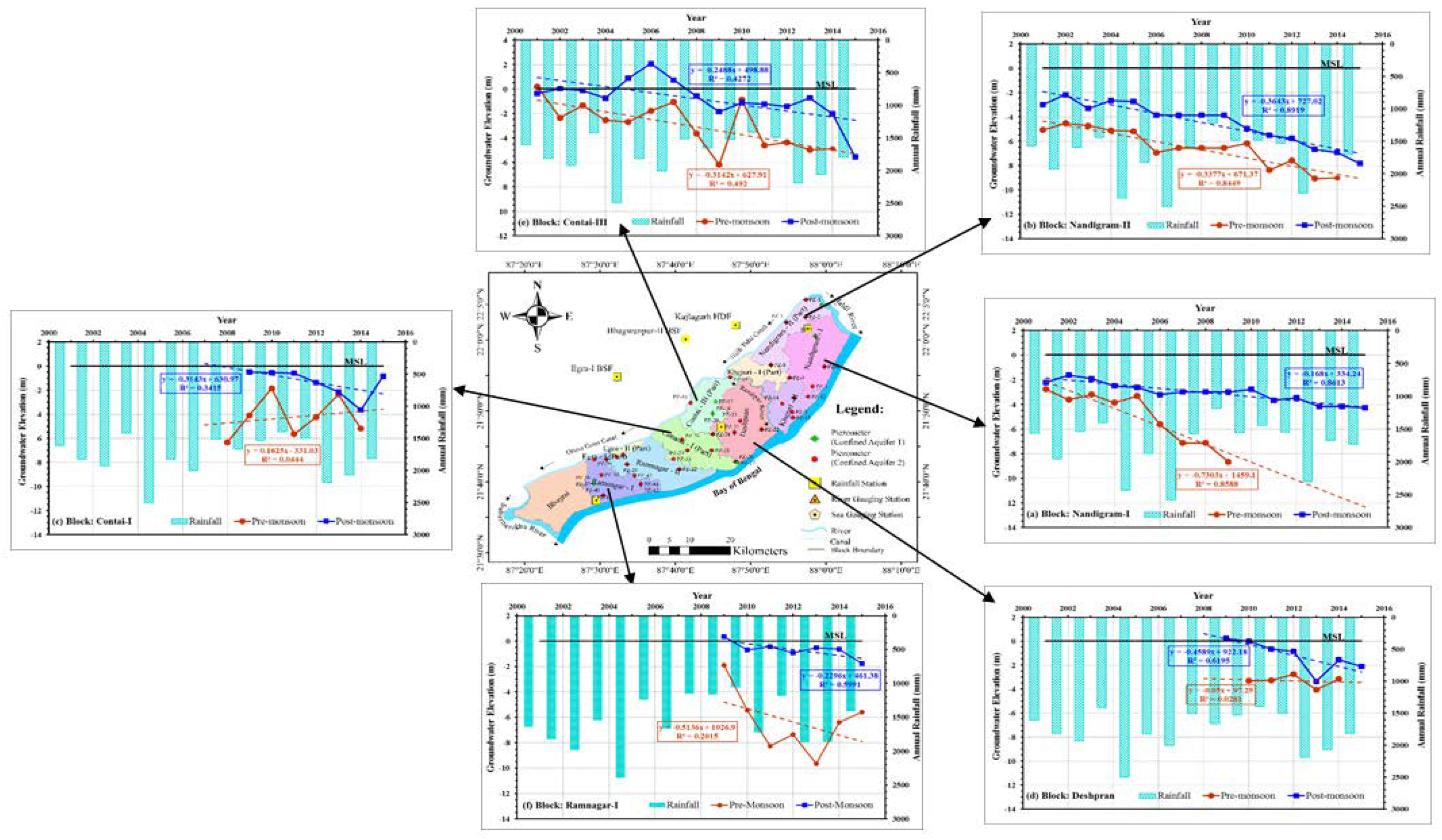
4.3.1. Groundwater Fluctuations in the Leaky Confined Aquifer
The pre-monsoon and post-monsoon groundwater-level time series data for 6 blocks are shown in Figure 2a–f along with the annual rainfall time series data. Among the 6 blocks, pre-monsoon and post-monsoon groundwater levels (GWL) are below the mean sea level (MSL) in Nandigram-I, Nandigram-II, and Contai-I blocks (Table 3).
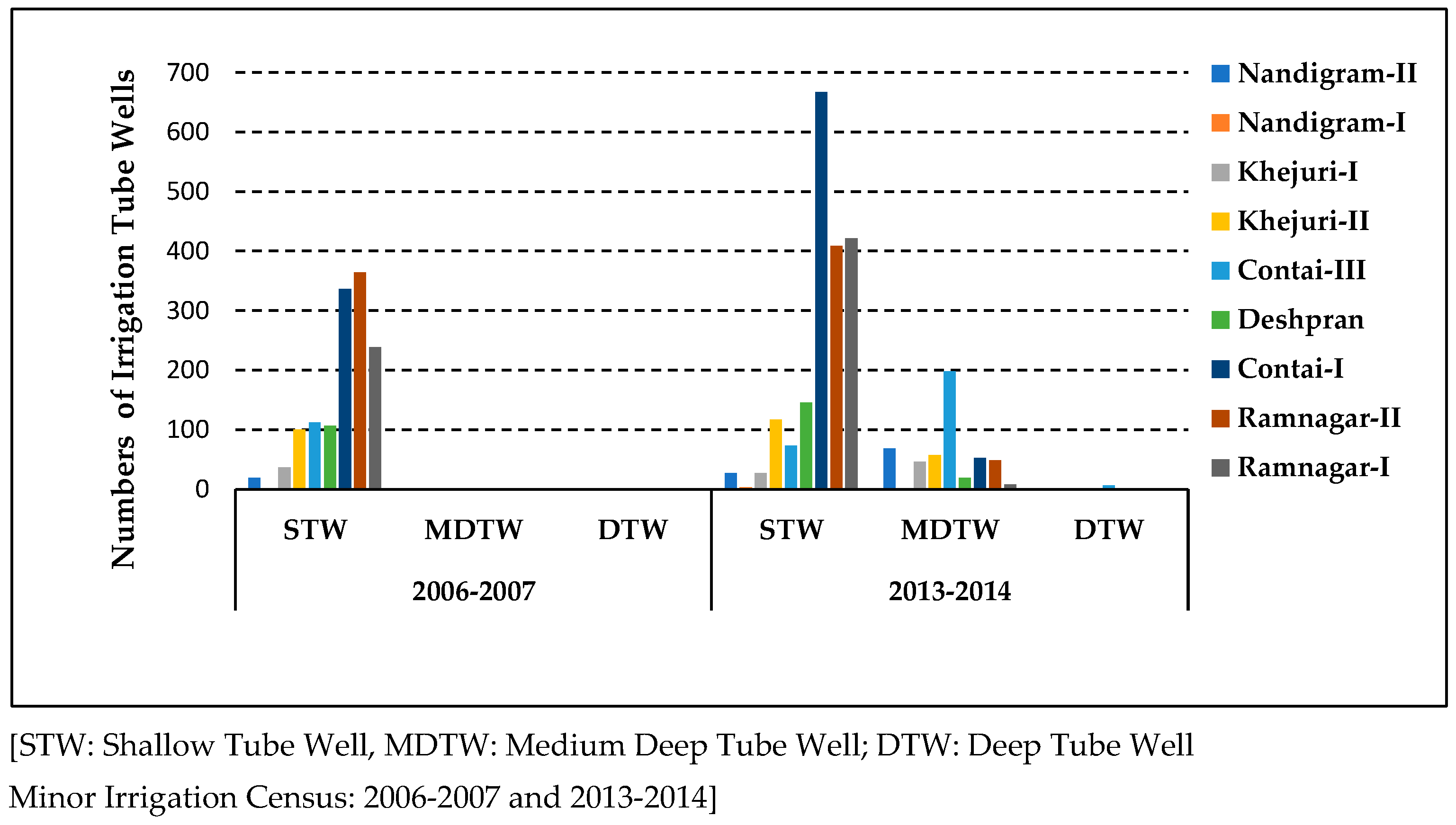
Overall, the pre-monsoon GWL varies from 0.18 to −9.07 m, whereas the post-monsoon GWL varies from 2.06 to −7.82 m. This should be because of enhancement of groundwater extraction due to an increased number of irrigation Shallow Tube Wells (STW) and additional installation of a good number of irrigation Medium Deep Tube Wells (MDTW) after 2006–2007 (Figure 3). It can be observed from Figure 2a–f that the North-East part shows a more decreasing trend in both pre-monsoon and post-monsoon seasons. Nandigram-I block has a less decreasing trend of groundwater level compared to Nandigram-II in the post-monsoon groundwater level, but Nandigram-I is more vulnerable to seawater intrusion as compared to Nandigram-II as it is located near to the sea. This might be due to withdrawal of a larger quantity of groundwater through greater numbers of MDTWs in Nandigram-II as compared to Nandigram-I. In the Central part of the study area, Contai-I and Contain-III have a more declining trend compared to Deshpran, as a result of heavy withdrawal of groundwater by a large number of MDTWs in Contai-I and Contai-III as compared to Deshpran (Figure 3). In the South-West part (Ramnagar-I), pre-monsoon groundwater level shows a declining trend, but it recovers during the post-monsoon season compared to other blocks.
4.3.2. Groundwater Fluctuations in the Confined Aquifer
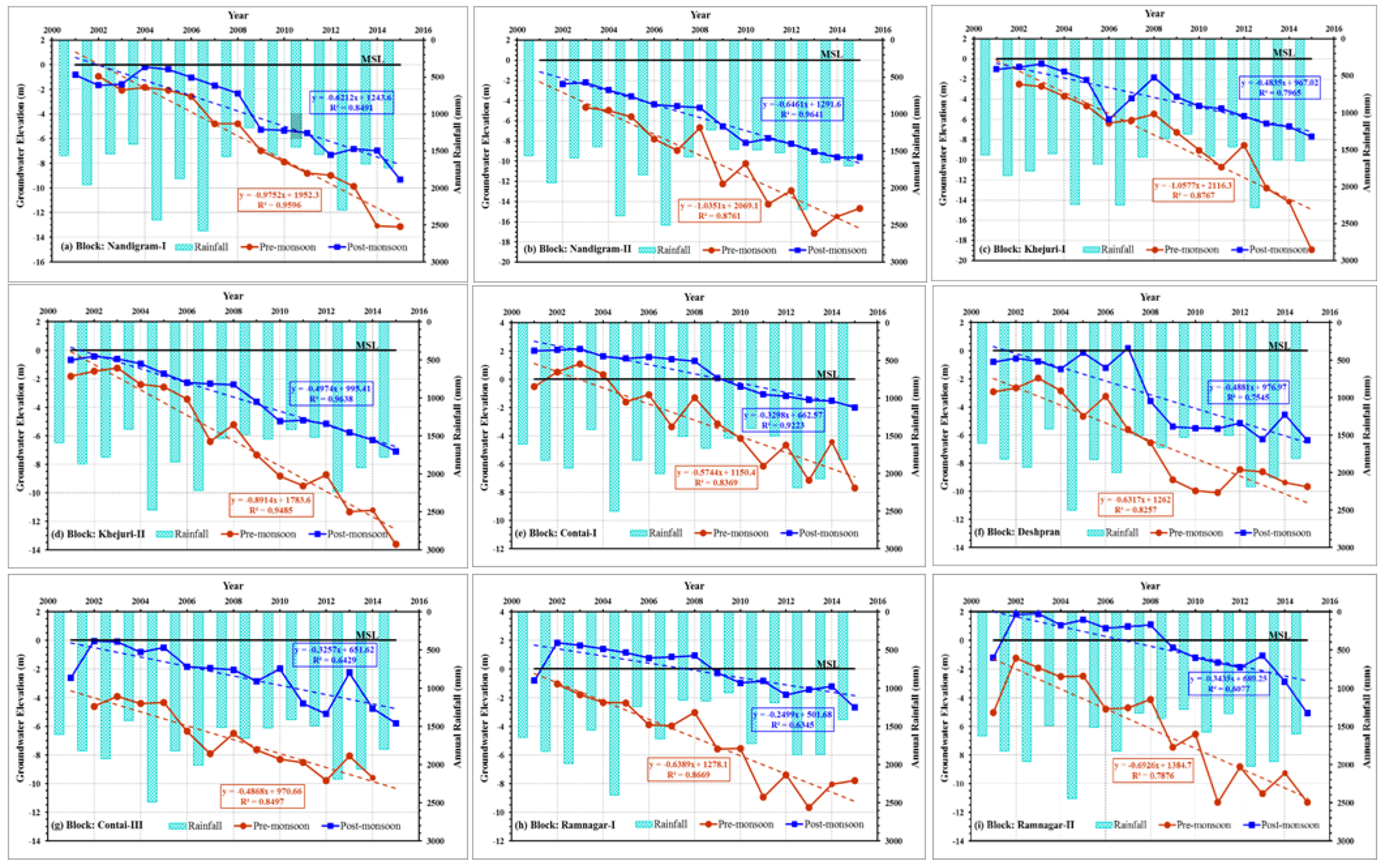
Pre-monsoon and post-monsoon groundwater-level data for 9 blocks are shown in Figure 4a–i along with annual rainfall. Among the 9 blocks, pre-monsoon and post-monsoon groundwater levels are below the mean sea level (MSL) in Nandigram-I, Nandigram-II, Khejuri-I, Khejuri-II, Deshpran, and Contai-III blocks (Table 4).
In Nandigram-I block, the pre-monsoon GWL in 2002 (−0.93 m) was higher than the post-monsoon GWL (Figure 4a). This is due to the fact that the graph was plotted for average GWL but pre-monsoon GWL data in 2002 are available only at one site. In Contai-I block, the pre-monsoon GWL is below MSL in 2001, afterward, it rises above MSL up to 2004, and then it declines up to 7.71 m below MSL in 2015. On other hand, the post-monsoon GWL is above MSL up to 2008 and then declines up to 1.99 m below MSL in 2015 (Figure 4e).
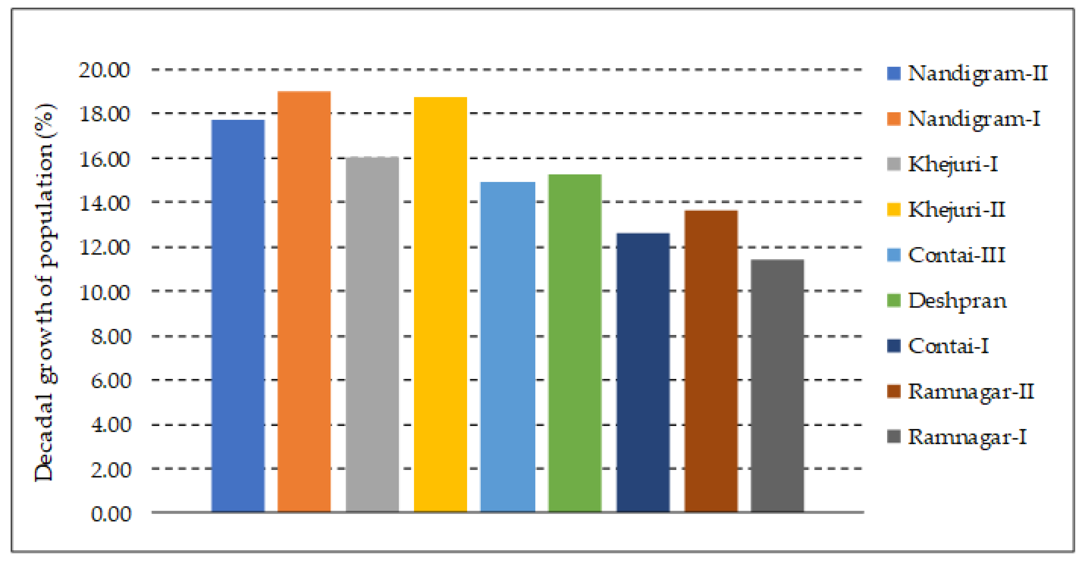
Post-monsoon groundwater levels of Ramnagar-I and Ramnagar-II are above MSL up to 2008, which decline up to 2.68 and 5 m below MSL, respectively, in 2015 (Figure 4h,i). From Figure 4a–i, The North-East part shows a greater decreasing trend in the groundwater levels of pre-monsoon and post-monsoon seasons as compared to other parts of the study area. The reason might be a larger groundwater withdrawal by Public Health Engineering Department (PHED), Government of West Bengal for domestic purpose by the higher growth rated (decadal) population in the northeastern part (16–18.97%) than the other part (11.40–14.88%) of the study area (Figure 5). In the Central part, Deshpran and Contai-III have a higher declining trend in groundwater levels in comparison to Contai-I. More groundwater withdrawal from additional installation of a few irrigation DTWs after 2006–2007 in confined aquifer of Contai-III, which may be the cause of higher declining trend. In the South-West part, the trends in the pre-monsoon and post-monsoon groundwater-levels of Ramnagar-II are greater than Ramnagar-I. The reason might be due to higher withdrawal of groundwater by PHED from the confined aquifer to fulfil the domestic water requirement for comparatively high growth rated population in Deshpran, Contai-III and Ramnagar-II as compared to Contai-I and Ramnagar-I (Figure 5).
4.4. Seawater Intrusion Status
The study area possesses high geologic heterogeneity. The pattern of variation of salinity measured as chloride (Cl−) and Total Dissolved Solids (TDS) concentration is heterogeneous in three-dimensional spaces. For better understanding of seawater intrusion, the study area was divided into three parts, i.e., North-East, Central, and South-West parts.
Chloride (Cl−) and TDS concentrations of groundwater in the leaky confined aquifer show remarkable spatial and temporal variations during 2011–2014. In Nandigram-I and Ramnagar-I, both the Chloride (Cl−) and TDS concentration in groundwater remains within the WHO guideline value i.e., <250 mg/L and <1000 mg/L, respectively (https://www.who.int/publications/i/item/9789241549950, accessed on 10 July 2018). During the pre-monsoon of 2014, Cl− concentration greater than 250 mg/L was found in Nandigram-II and Contai-I. In Deshpran, both the Cl− and TDS concentrations fluctuate seasonally and annually, and high Cl− and TDS concentrations were noticed during the pre-monsoon of 2014. Furthermore, in Contai-III block, Cl− and TDS concentrations are above the WHO guideline value.
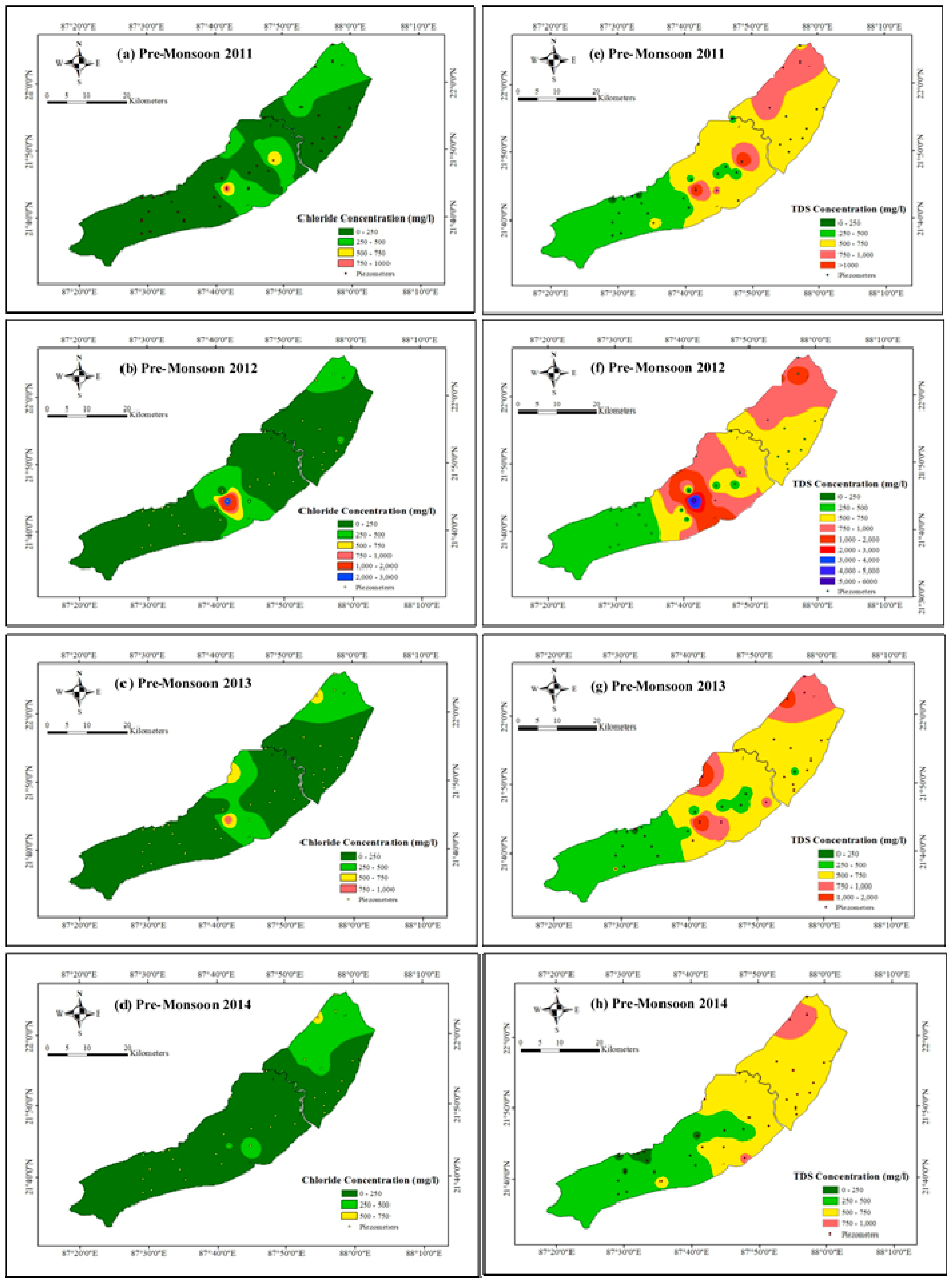
Significant spatial variation and comparatively higher concentration of Cl− and TDS in pre-monsoon groundwater were found in the confined aquifer (Figure 6a–h). The central part of the study area shows a higher concentration of Cl− (>250 mg/L) and TDS (>1000 mg/L) i.e., beyond the WHO guideline value. This is because of high tidal saline water ingress into the coastal aquifers through leakage from the beds of Rasulpur River (passing through Deshpran), Pichaboni Khal (passing through Contai-I), and Mirzapur Khal (connector of Rasulpur River and Pichaboni Khal; passing through both Deshpran and Contai-I). Furthermore, the confined aquifer in the North-East part (particularly in Nandigram-I and Nandigram II) shows high Cl− (>250 mg/L) and moderate TDS (750–1000 mg/L). This may be due to the saline water ingress through leakage from the Haldi River bed, and declining trend of groundwater level during both pre-monsoon and post-monsoon seasons.
Based on distribution of Chloride (Cl−) and TDS concentration in groundwater, it can be inferred that the effect of seawater intrusion is persistent in the leaky confined aquifer in Contai-III block (Central part of the study area). However, in Deshpran block, both the chloride and TDS concentrations fluctuate seasonally and annually. Mild effect of seawater intrusion is found in Nandigram-I, Nandigram-II, and Contai-I blocks. However, in Ramnagar-I, the effect of seawater intrusion is not markedly noticeable. This might be due to the presence of soil of low hydraulic conductivity of the aquifer in the area [26]. On the other hand, the effect of seawater intrusion is persistent in the confined aquifer in Nandigram-II block showing greater salinity than corresponding Nandigram-I block adjacent to the seacoast. This situation occurs as the filaments of high hydraulic conductivity interspersed with soil of low hydraulic conductivity protrude deep inland from the sea causing ingress of sea water inland through this preferential path (Maity et al., 2017) [29]. However, in the Central part of the study area (i.e., Contai-I, Deshpran, and Contai-III blocks), the concentrations of both Cl− and TDS in groundwater of confined aquifer vary considerably from season to season as well as from year to year.
5. Conclusions
The goal of the present study was to investigate the spatio-temporal characteristics of groundwater-level and evaluate the seawater intrusion status of the leaky confined and confined aquifers. For this, trend analysis of seasonal groundwater levels (i.e., pre-monsoon and post-monsoon seasons) was carried out by the Mann-Kendall test, Linear Regression test, and Innovative Trend test for both leaky-confined and confined aquifers. Thereafter, the fluctuations of pre-monsoon and post-monsoon groundwater levels with time and space were analyzed. As the groundwater levels during pre-monsoon and post-monsoon season decline below the mean sea level leading to a reversal of hydraulic gradient, it causes inland movement of seawater in aquifers of some coastal blocks and hence, they are vulnerable to seawater intrusion. By analyzing the chloride (Cl−) and TDS concentrations of groundwater, the status of seawater intrusion in the study area was evaluated. The methodology of this study can be useful for management of the groundwater resources in other coastal regions of India as well as other coastal parts of the world. Statistical analysis of available datasets supported with simulation-optimization modelling in this study area can be suggested for future research to address the seawater intrusion problem more efficiently.
Author Contributions
Conceptualization, S.H. and M.K.J.; Methodology, S.H., L.D. and M.K.J.; Software, L.D. and M.K.J.; Data curation, S.H., L.D. and M.K.J.; Writing—original draft preparation, S.H.; Writing—Review and editing, S.H., L.D. and M.K.J.; Supervision, M.K.J. All authors have read and agreed to the published version of the manuscript.
Funding
Not applicable.
Institutional Review Board Statement
Not applicable.
Informed Consent Statement
Not applicable.
Data Availability Statement
The data presented in this study are available on request from the corresponding author.
Conflicts of Interest
The authors declare no conflict of interest.
References
- Costanza, R.; Arge, D.R.; De Groot, R.; Ferber, S.; Grasso, M.; Hannon, B.; Limburg, K.; Naeem, S.; O’Neill, R.V.; Paruello, J.; et al. The value of the world’s ecosystem services and natural capital. Nature 1997, 387, 253–260. [Google Scholar] [CrossRef]
- Ferguson, G.; Gleeson, T. Vulnerability of coastal aquifers to groundwater use and climate change. Nat. Clim. Chang. 2012, 2, 342–345. [Google Scholar] [CrossRef]
- Shahin, M.; Van Oorschot, H.J.L.; De Lange, S.J. Statistical Analysis in Water Resources Engineering; A.A. Balkema: Rotterdam, The Netherlands, 1993; ISBN 9054101636. [Google Scholar]
- Sen, Z. Innovative trend analysis methodology. J. Hydrol. Eng. ASCE 2012, 17, 1042–1046. [Google Scholar] [CrossRef]
- Machiwal, D.; Jha, M.K. Comparative evaluation of statistical tests for time series analysis: Application to hydrological time series. Hydrol. Sci. 2008, 53, 353–366. [Google Scholar] [CrossRef]
- Ghosh, S.; Luniya, V.; Gupta, A. Trend analysis of Indian summer monsoon rainfall at different spatial scales. Atmos. Sci. Lett. 2009, 10, 285–290. [Google Scholar] [CrossRef]
- Duhan, D.; Pandey, A. Statistical analysis of long term spatial and temporal trends of precipitation during 1901–2002 at Madhya Pradesh, India. Atmos. Res. 2013, 122, 136–149. [Google Scholar] [CrossRef]
- Martinez, C.J.; Maleski, J.J.; Miller, M.F. Trends in precipitation and temperature in Florida, USA. J. Hydrol. 2012, 452, 259–281. [Google Scholar] [CrossRef]
- Jain, S.K.; Kumar, V.; Saharia, M. Analysis of rainfall and temperature trends in northeast India. Int. J. Climatol. 2013, 33, 968–978. [Google Scholar] [CrossRef]
- Awan, J.A.; Bae, D.H.; Kim, K.J. Identification and trend analysis of homogeneous rainfall zones over the East Asia monsoon region. Int. J. Climatol. 2015, 35, 1422–1433. [Google Scholar] [CrossRef]
- Kundu, S.; Khare, D.; Mondal, A.; Mishra, P.K. Analysis of spatial and temporal variation in rainfall trend of Madhya Pradesh, India (1901–2011). Environ. Earth Sci. 2015, 73, 8197–8216. [Google Scholar] [CrossRef]
- Oztopal, A.; Sen, Z. Innovative trend methodology applications to precipitation records in Turkey. Water Resour. Manag. 2016. [Google Scholar] [CrossRef]
- Sharma, C.S.; Panda, S.N.; Pradhan, R.P.; Singh, A.; Kawamura, A. Precipitation and temperature changes in eastern India by multiple trend detection methods. Atmos. Res. 2016, 180, 211–225. [Google Scholar] [CrossRef]
- Thomas, J.; Prasannakumar, V. Temporal analysis of rainfall (1871–2012) and drought characteristics over a tropical monsoon-dominated State (Kerala) of India. J. Hydrol. 2016, 534, 266–280. [Google Scholar] [CrossRef]
- Radhakrishna, I. Groundwater Systems Analysis of Indian Coastal Deltas: Resource Potentials, Quality Trends, Saline-Fresh Water Interrelationships and Management Strategies; BS Publications: Hyderabad, India, 2014; p. 572. [Google Scholar]
- Bhosale, D.D.; Kumar, C.P. Simulation of seawater intrusion in Ernakulam coast. In Proceedings of the International Conference on Hydrology and Watershed Management Vol. II, Hyderabad, India, 18–20 December 2002; pp. 390–399. [Google Scholar]
- Elango, L.; Sivakumar, C. Regional Simulation of a Groundwater Flow in Coastal Aquifer, Tamil Nadu, India. In Groundwater Dynamics in Hard Rock Aquifers; Ahmed, S., Jayakumar, R., Salih, A., Eds.; Springer: Amsterdam, The Netherlands, 2008; pp. 234–242. [Google Scholar]
- Datta, B.; Vennalakanti, H.; Dhar, A. Modeling and control of saltwater intrusion in a coastal aquifer of Andhra Pradesh, India. J. Hydro-Environ. Res. 2009, 3, 148–159. [Google Scholar] [CrossRef]
- Ganesan, M.; Thayumanavan, S. Management Strategies for a Seawater Intruded Aquifer System. J. Sustain. Dev. 2009, 2, 94–106. [Google Scholar] [CrossRef]
- Sindhu, G.; Ashitha, M.; Jairaj, P.G.; Raghunath, R. Modelling of coastal aquifers of Trivandrum. Procedia Eng. 2012, 38, 3434–3448. [Google Scholar] [CrossRef] [Green Version]
- Lathashri, U.A.; Mahesha, A. Predictive simulation of seawater intrusion in a tropical coastal aquifer. J. Environ. Eng. 2015, 142, D4015001-1. [Google Scholar] [CrossRef]
- Mohan, S.; Pramada, S.K. Management of South Chennai coastal aquifer system: A multi-objective approach. Jalvigyan Sameeksha 2015, 20, 1–14. [Google Scholar]
- Rejani, R.; Jha, M.K.; Panda, S.N.; Mull, R. Simulation modeling for efficient groundwater management in balasore coastal basin, India. Water Resour. Manag. 2008, 22, 23–50. [Google Scholar] [CrossRef]
- Goswami, A.B. A study of salt water encroachment in the coastal aquifer at Digha, Midnapore District, West Bengal, India. Int. Assoc. Sci. Hydrol. 1968, 13, 77–87. [Google Scholar] [CrossRef]
- Shrivastava, G.S. Impact of sea-level rise on seawater intrusion into coastal aquifer. J. Hydrol. Eng. ASCE 1998, 3, 74–78. [Google Scholar] [CrossRef]
- Bhattacharya, A.K.; Basack, S. Significance of hydrogeological and hydrochemical analysis in the evaluation of groundwater resources: A case study from the East Coast of India. Int. Organ. Sci. Res. J. Eng. 2012, 2, 61–71. [Google Scholar]
- Haan, C.T. Statistical Methods in Hydrology; Iowa State University Press: Ames, IA, USA, 1977. [Google Scholar]
- Hirsch, R.M.; Slack, J.R.; Smith, R.A. Techniques of trend analysis for monthly water quality data. Water Resour. Res. 1982, 18, 107–121. [Google Scholar] [CrossRef] [Green Version]
- Maity, P.K.; Das, S.; Das, R. Assessment of Groundwater Quality and Saline Water Intrusion in the Coastal Aquifers of Purba Midnapur District. Indian J. Environ. Prot. 2017, 37, 31–40. [Google Scholar]
Figure 1.
Location map of the study area with the locations of piezometers and gauging stations.

Figure 2.
(a–f) Groundwater-level fluctuations in the leaky confined aquifer during pre-monsoon and post-monsoon seasons and annual rainfall (2001–2015).
Figure 2.
(a–f) Groundwater-level fluctuations in the leaky confined aquifer during pre-monsoon and post-monsoon seasons and annual rainfall (2001–2015).

Figure 3.
Groundwater irrigation tube wells during 2006–2007 and 2013–2014.

Figure 4.
(a–i) Groundwater-level fluctuations in the confined aquifer during pre-monsoon and post-monsoon seasons and annual rainfall (2001–2015).
Figure 4.
(a–i) Groundwater-level fluctuations in the confined aquifer during pre-monsoon and post-monsoon seasons and annual rainfall (2001–2015).

Figure 5.
Decadal (2000–2001 to 2010–2011) growth rate of population.

Figure 6.
(a–h) Chloride (Cl−) and TDS distribution (2011–2014) in groundwater of confined aquifer.


Table 1.
Test-statistics of three selected trend tests for the pre-monsoon groundwater level of the leaky confined aquifer.
Table 1.
Test-statistics of three selected trend tests for the pre-monsoon groundwater level of the leaky confined aquifer.
| Block | Results of Trend Tests | ||||||||
|---|---|---|---|---|---|---|---|---|---|
| Mann-Kendall Test | Linear Regression Test | Innovative Trend Test | |||||||
| Calc. | Critical | Trend | Calc. | Critical | Trend | Calc. | Critical | Trend | |
| 1. Nandigram-I | −2.935 | ±1.96 | Yes | −6.524 | ±2.365 | Yes | 0.057 | ±0.074 | No |
| 2. Nandigram-II | −3.578 | ±1.96 | Yes | −8.084 | ±2.179 | Yes | −0.310 | ±0.054 | Yes ↓ |
| 3. Contai-I | −0.30 | ±1.96 | No | 0.481 | ±2.571 | No | −0.022 | ±0.034 | No |
| 4. Deshpran | 0.244 | ±1.96 | No | −0.294 | ±3.182 | No | −0.3 | 0 | Yes ↓ |
| 5. Contai-III | −2.408 | ±1.96 | Yes | −3.408 | ±2.179 | Yes | −0.365 | ±0.042 | Yes ↓ |
| 6. Ramnagar-I | −1.360 | ±1.96 | No | −2.295 | ±2.447 | No | −1.096 | ±0.322 | Yes ↓ |
Note: ↓ = Decreasing trend.
Table 2.
Test-statistics of three selected trend tests for post-monsoon groundwater level of the leaky confined aquifer.
Table 2.
Test-statistics of three selected trend tests for post-monsoon groundwater level of the leaky confined aquifer.
| Block | Results of Trend Tests | ||||||||
|---|---|---|---|---|---|---|---|---|---|
| Mann-Kendall Test | Linear Regression Test | Innovative Trend Test | |||||||
| Calc. | Critical | Trend | Calc. | Critical | Trend | Calc. | Critical | Trend | |
| 1. Nandigram-I | −3.982 | ±1.96 | Yes | −8.986 | ±2.160 | Yes | −0.156 | ±0.007 | Yes ↓ |
| 2. Nandigram-II | −4.402 | ±1.96 | Yes | −10.35 | ±2.160 | Yes | −0.389 | ±0.042 | Yes ↓ |
| 3. Contai-I | −2.103 | ±1.96 | Yes | −1.61 | ±2.571 | No | −01.458 | ±0.135 | Yes ↓ |
| 4. Deshpran | −2.403 | ±1.96 | Yes | −2.853 | ±2.571 | Yes | −0.611 | ±0.163 | Yes ↓ |
| 5. Contai-III | −2.771 | ±1.96 | Yes | −3.114 | ±2.160 | Yes | −0.330 | ±0.104 | Yes ↓ |
| 6. Ramnagar-I | −1.502 | ±1.96 | No | −2.733 | ±2.571 | Yes | −0.097 | ±0.057 | Yes ↓ |
Note: ↓ = Decreasing trend.
Table 3.
Temporal variation of groundwater level in leaky confined aquifer.
| Block | Groundwater Level within 2001–2015 (m MSL) | |
|---|---|---|
| Pre-Monsoon | Post-Monsoon | |
| 1. Nandigram-I | −2.76 to −8.66 | −1.61 to −4.26 |
| 2. Nandigram-II | −4.52 to −9.07 | −2.17 to −7.82 |
| 3. Contai-I | −1.84 to −6.34 | −0.49 to −3.64 |
| 4. Deshpran | −2.76 to −4.06 | 0.24 to −3.36 |
| 5. Contai-III | 0.18 to −6.19 | 2.06 to −5.55 |
| 6. Ramangar-I | −1.89 to −5.59 | 0.36 to −1.79 |
Table 4.
Temporal variation of groundwater level in confined aquifer.
| Block | Groundwater Level within 2001–2015 (m MSL) | |
|---|---|---|
| Pre-Monsoon | Post-Monsoon | |
| 1. Nandigram-I | −0.93 to −13.16 | −0.18 to −9.33 |
| 2. Nandigram-II | −4.67 to −17.17 | −2.19 to −9.62 |
| 3. Khejuri-I | −2.51 to −18.91 | −0.46 to −7.71 |
| 4. Khejuri-II | −1.24 to −13.62 | −0.42 to −7.08 |
| 5. Contai-I | 1.09 to −7.71 | 2.16 to −2.00 |
| 6. Deshpran | −1.96 to −10.10 | 0.18 to −6.37 |
| 7. Contai-III | −3.90 to −9.77 | −0.05 to −5.77 |
| 8. Ramnagar-I | −1.04 to −9.67 | 1.83 to −2.68 |
| 9. Ramnagar-II | −1.24 to −11.31 | 1.86 to −5.06 |
Publisher’s Note: MDPI stays neutral with regard to jurisdictional claims in published maps and institutional affiliations. |
© 2021 by the authors. Licensee MDPI, Basel, Switzerland. This article is an open access article distributed under the terms and conditions of the Creative Commons Attribution (CC BY) license (https://creativecommons.org/licenses/by/4.0/).
Share and Cite
MDPI and ACS Style
Halder, S.; Dhal, L.; Jha, M.K. Investigating Groundwater Condition and Seawater Intrusion Status in Coastal Aquifer Systems of Eastern India. Water 2021, 13, 1952. https://doi.org/10.3390/w13141952
AMA Style
Halder S, Dhal L, Jha MK. Investigating Groundwater Condition and Seawater Intrusion Status in Coastal Aquifer Systems of Eastern India. Water. 2021; 13(14):1952. https://doi.org/10.3390/w13141952
Chicago/Turabian StyleHalder, Subrata, Lingaraj Dhal, and Madan K. Jha. 2021. "Investigating Groundwater Condition and Seawater Intrusion Status in Coastal Aquifer Systems of Eastern India" Water 13, no. 14: 1952. https://doi.org/10.3390/w13141952
Note that from the first issue of 2016, this journal uses article numbers instead of page numbers. See further details here.