
A Unified View of Nonlinear Resistance Formulas for Seepage Flow in Coarse Granular Media


1
Department of Civil Engineering, Hydraulics, Energy and Environment, E.T.S. de Ingenieros de Caminos, Canales y Puertos, Universidad Politécnica de Madrid (UPM), Profesor Aranguren s/n, 28040 Madrid, Spain
2
SERPA Dam Safety Research Group, Department of Civil Engineering, Hydraulics, Energy and Environment, E.T.S. de Ingenieros de Caminos, Canales y Puertos, Universidad Politécnica de Madrid (UPM), Profesor Aranguren s/n, 28040 Madrid, Spain
3
Centre Internacional de Metodes Numerics en Enginyeria (CIMNE), Campus Norte UPC, Gran Capitán s/n, 08034 Barcelona, Spain
*
Author to whom correspondence should be addressed.
Water 2021, 13(14), 1967; https://doi.org/10.3390/w13141967
Submission received: 17 May 2021
/
Revised: 1 July 2021
/
Accepted: 6 July 2021
/
Published: 17 July 2021
(This article belongs to the Special Issue Dam Safety. Overtopping and Geostructural Risks)
Abstract
:There are many studies on the nonlinear relationship between seepage velocity and hydraulic gradient in coarse granular materials, using different approaches and variables to define the resistance formula applicable to that type of granular media. On the basis of an analysis of the existing formulations developed in different studies, we propose an approach for comparing the results obtained by some of the most important studies on state-of-the-art seepage flow in coarse granular media.
1. Introduction and Objectives
It is essential to know the relationship between filtration speed and hydraulic gradient to understand the interactions that occurs between infiltrated water and structures composed of gravel or rockfill, such as dams, levees, drainage structures, and coastal dikes. These porous media, made up of coarse particles, possess special characteristics due to their large pores which, under certain conditions, may give rise to non-laminar seepage flow, invalidating Darcy’s Law. Calculating the seepage flow through this type of porous media requires the use of so-called nonlinear resistance formulas. The flow regime in which this is applied is known as non-Darcy flow.
Various nonlinear relationships have been proposed to describe the flow in coarse porous media. They can be grouped into two types of equations as follows:
where V is the seepage velocity, defined as the average fluid velocity in the whole transversal section; is the hydraulic gradient; and are parameters depending on the characteristics of the porous medium and of the fluid; is only a function of the characteristics of the porous medium; and is a function parameter of the conditions of the flow.
Equation (1) is the so-called exponential equation and Equation (2) is the quadratic equation. To obtain relationships among the parameters , , , and , different physical parameters have been considered; experimental data with different intervals of size, shape, and particle angularity have been used, as well as a wide range of gradient intervals. However, there is currently no formula that can completely create Equations (1) and (2) and combine the determination criteria of their coefficients based on physical parameters.
In order to have a unified vision of the relationships between gradients and seepage velocity developed in different studies, we conduct an analysis of the existing formulations and identify similarities by mathematically comparing the physical parameters considered in these studies. These relationships make it easier to compare the results and formulations obtained by each of the studies considered in this article.
2. Review of Resistance Formulas in Nonlinear Porous Media
2.1. Conceptual Approach
Various studies have been completed with the aim of developing expressions for parameters (linear coefficient) and (quadratic coefficient) of Forchheimer’s Law (1901) [1] Equation (2), which defines a macroscopic hydraulic behaviour. The first term of Equation (2) (i.e., the term with coefficient ) represents the loss of energy due to the viscous forces and depends on the properties of both the porous medium and the fluid. The second term of Equation (2) (i.e., the term with coefficient s) considers the loss of energy due to the forces of inertia, and depends only on the properties of the porous medium.
In most of these studies, the development of formulas was based on the analogy of the flow in pipes, through the application of two dimensionless groups that, in this paper, are referred to as the generalised friction factor of the Darcy–Weisbach Equation (3) and generalised Reynolds number Equation (4) represented as:
where is the characteristic length adopted in each case, is the gravitational acceleration, is the hydraulic gradient, is the kinematic viscosity, and is the pore velocity, determined by Equation (5):
being the porosity of the porous medium.
The characteristic lengths, on which most studies have been based, can be grouped into three types:
- (a)
- the representative size of the particle ()
- (b)
- the square root of the intrinsic permeability (), as a macroscopic property of the porous medium. For the laminar regime, it is determined by Equation (6):
- (c)
- the hydraulic mean radius that was first defined by Taylor (1948) [2] and determined by Equation (7):where is the average specific surface area of the solid particles that make up the porous medium and depends on the shape, angularity, and surface roughness of the particles (Crawford, C.W. et al., 1986 [3]; Sabin G.C.W. and Hansen D., 1994 [4]) and is defined by the Equation (8):where SP is the average particle surface area and VP is the average particle volume.
Among the first studies are those developed by Blake (1922) [5] and S.P. Burke and W.B. Plumer (1928) [6], who used dimensionless groups defined by Equations (3) and (4), adopting as the characteristic length, and as the specific surface area of the packing of porous medium. The relationship with the average particle specific surface area determined by Equation (9) as follows:
In their tests, they used commercial porous media (glass beads, glass rings, solid glass cylinders, and Raschig rings), and the experimental data corresponding to a porous medium with the same geometry and size. The results were represented a generalised diagram [, Equation (10) and the values fitted to a smooth curve:
where is referred to as a linear generalised dimensionless coefficient, and as a quadratic generalised dimensionless coefficient.
Equation (10) is referred to as a generalised equation .
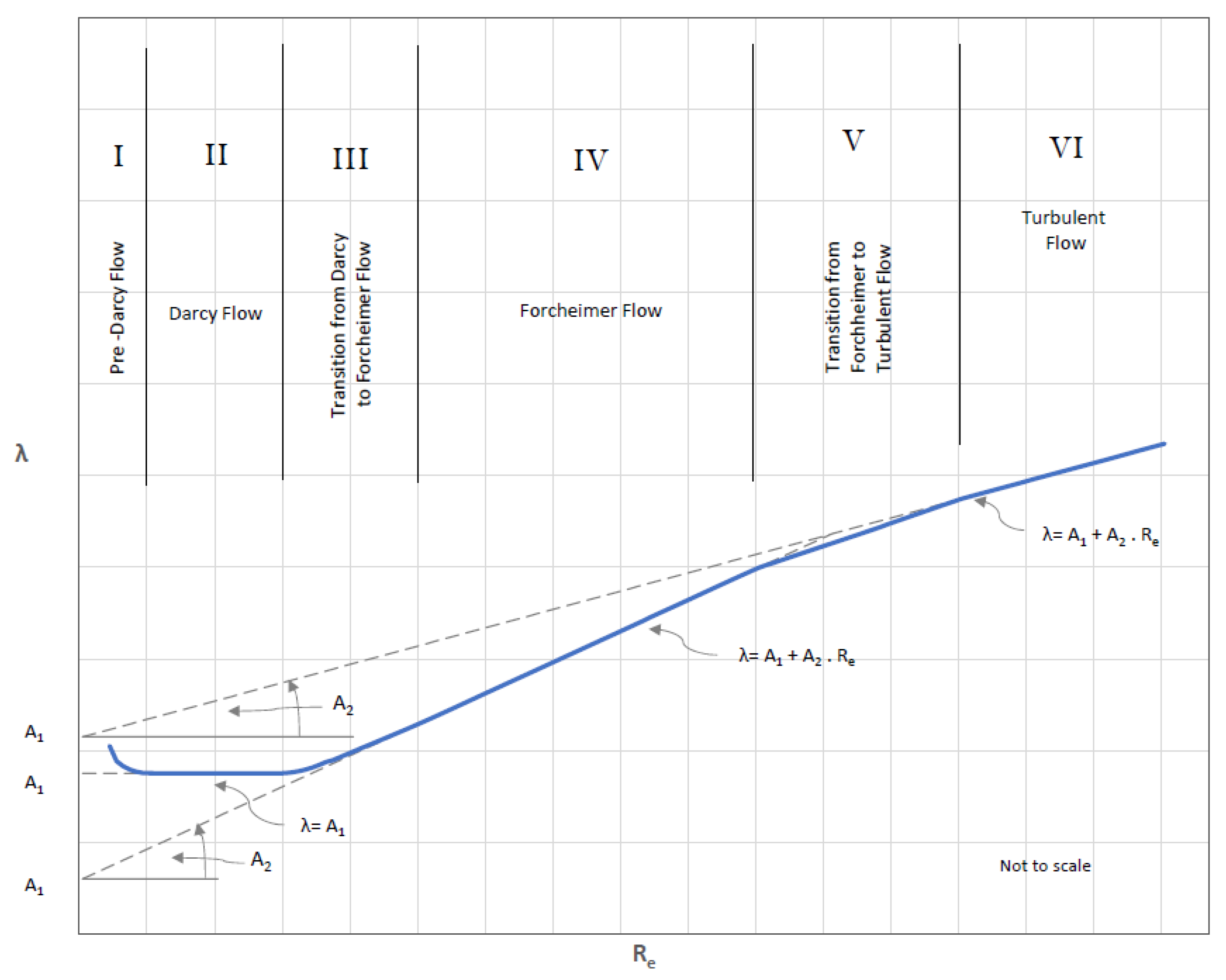
Figure 1 shows a [], schematic diagram similar to that used by Bear (1988) [7] with asymptotic values for increased Reynolds numbers .
As indicated by Sabri Ergun and A. A. Orning (1949) [8] “This transition from the dominance of viscous to kinetic effects, for most packed systems, is smooth, indicating that there should be a continuous function relating pressure drop to flow rate.”
Ward (1964) [9] stated the same thing when he asserted, “The smooth transition from laminar to turbulent flow in porous media is expected. In the laminar flow region, the flow is laminar in all parts of the porous media. In the laminar transition region, the flow is laminar in most parts of the porous medium, but there are parts where the flow is turbulent. In the turbulent transition region, the flow is turbulent in most parts of the porous medium, but there are still parts where laminar flow conditions persist. Finally, turbulent flow exists in all parts of the porous medium at high values of . Simultaneous existence of laminar and turbulent flow in different parts of a porous medium is possible because of the irregularities and variation in pore size.”
Dudgeon (1966) [10] indicated that “the only likely solution to the problem of a generalised plot is in terms of a set of graphs for each family of geometrically similar porous media.”
Other authors (Blake (1922) [5] and S.P. Burke and W.B. Plumer (1928) [6]; Morcon A.R. (1946) [11]; Ergun (1952) [12], Kadlec, H.R., and Knight, L.R. (1966) [13]; Ahmed and Sunada (1969) [14]; Kovacs (1969) [15], Arbhabhirama and Dinoy (1973) [16]; Stephenson (1979) [17]; Li, B et al. (1998) [18];and more recently Sidiropuolou et al. (2007) [19]; Moutsopoulos et al. (2009) [20]; Sedghi-Asl and Rahimi (2013) [21]; and Salahi et al. (2015) [22]), obtained continuous curves such as those given by Equation (10) through the corresponding adjustment of the experimental data used, always within the range of the Reynolds number on which the tests were developed.
The existence of these continuous curves in porous media contrasts with the turbulent flow in pipes where there are sudden jumps in the Reynolds number interval between 2000 and 4000 (White, F.W. (2003) [23]).
If we substitute the generalised values of and , given by Equations (3) and (4) in Equation (10) we get Equation (11):
Resolving in Equation (11) we get what we refer to as a quadratic generalised equation, i.e., Equation (12):
In accordance with the Equation (12) the parameters and of the Forchheimer equation, i.e., Equation (2) determine Equations (13) and (14):
In the case of the fully developed turbulent regime, it may be possible to disregard the linear expression , in such a way that we could obtain the exponential equation, Equation (2), considering the coefficient a as equal to the quadratic expression and the exponent as equal to 2.
Various researchers have worked on the exponential law, Equation (1), in regimes of transition, and therefore with the exponent values b below 2: Wilkins (1956) [24], b = 1.85; Dudgeon (1966) [10], 1.2 < b < 1.91; Parkin (1991) [25], b = 1.85; Moutsopoulos K. N. et al. (2009) [20], 1.280 < b < 1.687; Sedhi-Asl et al. (2013) [21] 1.479 < b < 1.804.
In this respect, Stephenson (1979) [17] pointed out the fact that not obtaining an adjustment of equal to 2, with the experimental data, is due to “the tests being carried out on a small scale and as a result of low Reynolds numbers.” Ferdos, F. et al. (2015) [26] obtained an exponent equal to 2 in their tests as a result of using elevated Reynolds numbers . These studies both used the particle Reynolds number determined by Equation (15) as follows:
They achieved values of = 220,000 for the size interval of 100–160 mm and = 320,000 for the range of 160–240 mm. The values were both very much higher as compared with the value proposed by Stephenson (i.e., Rd = 10,000) in order to reach the fully developed turbulent flow.
It is important to consider that the flow through for highly permeable porous media may contain various flow regimes, as the generalised Reynolds number increases. In general, most of the studies have shown that there are four flow regimes: laminar, nonlinear laminar, turbulent transition, and fully developed turbulent flow (Ward, 1964 [9]; Wright (1968) [27]; Kovacks (1969) [15], Dybbs and Edwards (1975) [28]; R.M. Fand et al. (1987) [29]; H. Huang and S. Ayoub (2007) [30]) and, consequently, there is a debate regarding whether the dimensionless coefficients and considered in Equations (10) and (12) for a determined porous medium, are constants throughout a wide range of seepage velocity spanning the four flow regimes, in other words maintaining the relationship determined by Equation (10) without producing sudden jumps as occurred in the flow in tubes.
For that purpose, it is interesting to linearise Equation (10) multiplying both parts of the equation by to obtain Equation (16):
where , the linearised generalised friction faction, is determined by Equation (17):
Equation (16) is referred to as a linearised generalised equation .
Figure 2 shows a diagram similar to that used by R.M Fand et al. (1987) [29]. In accordance with Equation (16), each porous material is represented by a line whose curve corresponds with the quadratic generalised dimensionless coefficient ; the cut on the ordinate axis corresponds to the linear generalised dimensionless coefficient . The laminar regime is represented by a horizontal line. This type of graph is used to check if, for the same porous material, each non-Darcy flow regime remains determined by their corresponding value pairs or, on the contrary, such values are constant for the three non-Darcy flow regimes.
In this debate, the following studies stand out: McCorquodale et al. (1978) [31] and Fand et al. (1987) [29]. The first group used granular materials, of various sizes, shapes, and angularity, whereas the second worked with spheres with a range of sizes from 2.00 mm < D < 4.00 mm. The studies both proposed different coefficient values, and , for the transition zones that they detected in their tests: nonlinear laminar and turbulent transition.
2.2. Resistance Formulas
Next, we describe the main nonlinear resistance formulas based on the adopted characteristic length .
2.2.1. Resistance Formulas Based on the Representative Diameter of the Particles
In 1952, Sabri Ergun [12] carried out a study to develop a formula for general application based on the dimensionless groups:
where is Ergun’s friction factor and is Ergun’s Reynolds number. The parameter was adopted as the representative diameter of the particles, that is, the average effective diameter of the granular material and determined by Equation (20):
where corresponds with the diameter of a sphere that has the same specific surface area, , as the particle.
The continuous curve, as determined by Equation (10) and defined by the author, we refer to it as the Ergun equation as follows:
where is the linear dimensionless coefficient and is the quadratic dimensionless coefficient (by Sabri Ergun and A. A. Orning).
Finally, substituting the values of and of Equations (18) and (19) into Equation (21) we get the quadratic equation from Ergun (1952) [12] as Equation (22):
This equation proposed by Ergun (1952) [12] had, in fact, been previously developed by Sabri Ergun and A. A. Orning (1949) [8] who adopted as characteristic length , the specific surface area of the particles . The equation is obtained by substituting in Equation (22) the value of the effective diameter defined by Equation (20). These authors developed this equation based on Kozeny’s (1927) hypothesis [32], which is based on a capillary model that, as the authors show “the granular bed is equivalent to a group of parallel and equal-sized channels, such that the total internal surface and the free internal volume, are equal to the total packing surface area and the void volume, respectively, of the randomly Packed bed.” However, they added that “For a packed bed, the flow path is sinuous, and the stream lines frequently converge and diverge. The kinetic losses, which occur only once for the capillary, occur with a frequency that is statistically related to the number of particles per unit length. For these reasons, a correction factor must be applied to each term. These factors may be designated as α and β.” For these reasons, in agreement with the authors, it is essential to consider some correction factors in each linear and quadratic expression of Equation (22) to consider these characteristics of the porous medium. The authors designated them as and , respectively.
Equation (22) considers the existence of a function of porosity for each expression: for the linear expression () and for the quadratic expression () of Equation (2) where:
As per Ergun, Leva M., and Grimmer M. (1947) [33] they confirmed these functions of porosity. Ergun himself carried out various tests on a wide range of porosity variation to check the validity of these functions.
With respect to the shape, angularity, and surface roughness of the particles, these physical parameters seem implicit in the effective diameter, , which relate to the specific surface area Se through Equation (20).
Finally, with respect to the packed porous material he indicates that “the orientation of the randomly packed beds is not susceptible to exact mathematical formulation”, and, consequently, “the effect of the orientation was not included.”
Ergun, worked on 640 experiments including his own, made up of crushed porous solids, and those obtained through other authors such as Burke and Plummer (1928) [6], who worked with lead shot (spherical shape) of reduced sizes 1.48, 3.08, and 6.34 mm and Morcon (1949) [11], who worked with capsules, cylinders, nodules, and spheres. Ergun represented the three series of data in the diagram checking that they correctly matched Equation (21) The fluids used in this case were the gases of CO2, N2, CH4, and H2. As a result of this, he obtained the universal values of = 2.08 and = 2.33 applicable to all porous media.
According to Ergun, most dispersions happen with porous materials that include a mixture of sizes (non-uniform materials), and with those in which the relationship between the diameter of the permeameter () and the representative size of the particle is less than 10 (influence of the wall effect). In such cases, the corresponding tests were not considered.
Although the author did not analyse the theoretical significance of the parameters and , he did confirm that over a wide range of porosities he found no relationships of and with the porosity.
Later, Frank Engelund (1953) [34] carried out a study to analyse the influence of turbulence in subterranean waters on uniform limestone sands, working on his own tests and those of other authors (Lindquist, 1933 [35] and Chardabellas, 1940 [36,37]). For his tests, he worked only on three samples, two of them were with = 2.6 mm and one with = 1.4 mm. The proposed quadratic equation Equation (25) was:
He used as the representative diameter of particle the parameter , which is the equivalent diameter that corresponds to the diameter of a sphere with the same volume of the particle; α0 is the linear dimensionless coefficient of Engelund and is the quadratic dimensionless coefficient of Engelund. According to the author, “ and are dimensionless numerical constants depending, for uniform soil, on the structure and the grain shape.”
The structure of Equation (25) is remarkably similar to Equation (22) given by Ergun (1952) [12]. The difference in the representative diameter of the adopted particle, by Ergun (1952) [12] and by Engelund (1953) [34], and the function of linear porosity obtained as:
According to Frank Engelund (1953) [34], this porosity function of the linear expression fits better than the function from Ergun Equation (23) to the measurements obtained by Rose (1953) [37] and Franzini (1951) [38], especially the latter, who worked with a wide interval of porosities 0.270 < n < 0.476.
Ergun (1952) [12] proposed universal values for the dimensionless coefficients and . However, Engelund (1953) [34] did consider the shape and angularity of the particles through the dimensionless coefficients and for which he proposed the following values:
= 780 for uniform spherical particles (using data from Lindquist (1933)); = 1000 for uniform rounded sands (using data from Chardabellas (1940)), and = 1500 or above for angular sands, (using own experimental data).
= 1.8 for uniform spherical particles (using data from Lindquist (1933)); = 2.8 for uniform rounded sands (using data from Chardabellas (1940)), and = 3.6 or above for angular and uniform sands, (using own experimental data).
Finally, we must point out that it is simpler to measure as representative diameter of the particle the value of than the value of , which requires the measurement of the particle specific surface area in accordance with Equation (20).
In 1979, Stephenson carried out a study whose main purpose was to research the fully developed turbulent flow regime. On the basis of an analogy with the flow in pipes (Darcy–Weisbach equation), he considered that the gradient was proportional to the expression Equation (27):
As the hydraulic mean radius is proportional to the size of the particle (Leps (1973)) [39] and, furthermore, this variable is more easily measured, he suggested using the exponential equation, i.e., Equation (1) with coefficient b equal to 2 for Equation (28):
where is the particle friction factor and, as the author noted, “is actually the function of the Reynolds number ”. The author used as the representative diameter of the particle , the parameter D50 for lack of other data in the bibliography. However, for conceptual reasons, we will continue working with the representative diameter of the particles .
He considered the dimensionless groups [] where:
and is defined by the Equation (15).
He represented the data of three types of porous materials: smooth spheres, river gravel, and crushed aggregates on the diagram from Stephenson (1979) [17] []. This data came from tests carried out by the same author and by various researchers: Dudgeon (1966) [10], Volker (1969) [40], Leps (1973) [39], and Cedergren (1977) [41]. With this experimental data and their corresponding ranges of particle sizes and hydraulic gradients, he matched three smooth curves whose lines coincided in the laminar regime. From this line, they gradually separate in the transition regime towards turbulence with three asymptotic values: d = 1 for smooth spheres, d = 2 for river gravel, and d = 4 for crushed aggregate (see Figure 3).
For laminar flow, considering the analogy with the flow in pipes and based on data from Dudgeon (1966) [10] and Cedergren (1977) [41], he proposed the relationship:
where is the linear dimensionless coefficient from Stephenson (1979) [17]. The value of obtained from the experimental data was 800. The limit of the Reynolds number for the laminar regime proposed by Stephenson was = 10−4.
In the transition zone, he proposed Equation (31) of the type given by Equation (10):
where is the quadratic dimensionless coefficient from Stephenson (1979) [17]. According to the author, Reynolds numbers of > 10,000 produce the fully developed turbulent flow regime and, in this case, the author indicated that it was only a function of the shape and angularity of the particles.
Ultimately, Equation (31) (similar to the generalised equation Equation (10)), the Ergun equation, i.e., Equation (21), and by implication Equation (25) by Frank Engelund, represent continuous curves for each porous medium in a generalised diagram [Re,] that tend to an asymptotic value for fully developed turbulent regime (see Figure 1 and Figure 3).
Finally, substituting Equations (15), (29) and (31), we get the quadratic equation Equation (32):
Equation (32), according to Li B. et al. (1998), was not initially proposed by Stephenson (1979) [17] and these authors termed it as the modified Stephenson equation.
2.2.2. Resistance Formulas Based on Intrinsic Permeability
Ward (1964) [9] obtained a quadratic formula for general application taking as the characteristic length. For this, he worked with the dimensionless groups expressed in Equations (33) and (34):
where is Ward’s friction factor and is Ward’s Reynolds number.
For the transition zone, in a diagram of the type produced by Equation (10), Ward (1964) [9] proposed Equation (35):
where is the quadratic dimensionless coefficient of Ward which, as indicated by Ahmed and Sunada (1969) [14], “Previous investigators have interpreted the term as a constant reflecting geometric properties of the medium.”
Considering the three previous equations, the author obtained the quadratic equation, i.e., Equation (36):
Ward (1964) [9] had the same aim as Ergun (1952) [12], to adjust a single value of so that Equation (35) might be generally applicable. Engelund (1953) [34], and Stephenson (1979) [17], in fact, proposed three equations also for general application, but depending on the structure of the porous material and the shape of the particles.
Ward (1964) [9] used 20 different porous media: glass bead, ion exchange resin, sands, gravel, granular activated carbon, and anthracite. The size of each porous medium was defined through the geometric mean of the particle sizes in each porous medium. The size interval was 0.27 mm < < 16.10 mm. In total, 53 tests were carried out and the fluid used was water. The Reynolds number interval was 0.122 < < 18.10, with the size interval of studied, he obtained an adjusted value for of 0.55 with a standard deviation of 0.024.
The author noted that “D.K. Todd (1959) [42] showed a plot similar to Figure 1, except that an average grain diameter is used in place of the square root of the permeability in Equations (10) and (16). Because the average grain diameter is not sufficient to characterize a porous medium, there is considerable scatter in the plotted points.”
Regardless of the existence of the smooth transition curve (see Figure 1), Ward (1964) [9] proposed, for engineering applications, the division into four types of flow regimes: laminar, nonlinear laminar, turbulent transition, and fully developed turbulent; with the following limits of the Reynolds number among them: laminar < 0.0182, nonlinear laminar < 1.82, and turbulent transition < 182.
To conclude, we must point out that Ward attributes, in some cases, the deviations seen in respect of Equation (35) to an inadequate determination of the intrinsic permeability , which must be obtained with very low gradients to be in a laminar regime in accordance with Equation (6).
Continuing with Ward’s study (1964) [9], Ahmed and Sunada (1969) [14] developed the same quadratic equation, i.e., Equation (36) from the Navier–Stokes’ equations, based on the hypothesis that the porous medium is homogeneous and isotropic on a macroscopic scale, and that the chemical and thermodynamic effects are small. His study focused specifically on the nonlinear laminar regime.
Ahmed and Sunada (1969) [14] stated that “for flow through porous media, convective accelerations are always present, whereas turbulence is a random phenomenon dependent upon of flow velocity and space geometry.” According to the authors, “This fact was demonstrated experimentally by Schneebeli (1955) [43] who used dye to identify the flow. He injected dye into the flow at various velocities (steady-state conditions) and found that, even though measurements of gradients and velocities indicated nonlinear flow, the dye assumed laminar characteristics, i.e., stream-lined flow. Increasing the flow velocities approximately four times caused the dye from one channel to mix with the dye of another, indicating that departure from Darcy’s Law should be the result of convective acceleration of the fluid within the pores space.”
More recently, H. Huang and J. Ayoub (2007) [30], concluded, “Derivation of the Forchheimer equation from the Navier–Stokes’ equation reveals that the nature of the Forchheimer flow regime is laminar with inertial effect. The inertia resistance factor β can be used to characterize this flow regime and is therefore an intrinsic property of the porous media.”
Along the same lines, Balhoff, M.T. et al. (2009) [44] indicated, “The constant, β, is referred to us as the non-Darcy coefficient and, like permeability, is an empirical value specific to the porous medium. It represents the additional inertial resistance caused by the converging/diverging and tortuous medium geometry.”
The phenomenon of the turbulence in porous media is very complex. Recently, Sidiripoulou, M.G. et al. (2007) [19] referred to studies by Skjetne and Auriault (1998) [45], Panfilov et al. (2003) [46], and Fourar et al. (2004) [47] on the mechanisms of turbulence, which were related to the separation of the layer limit and the recircularisation of the vortices formed.
2.2.3. Resistance Formulas Based on the Hydraulic Mean Radius
In 1998, Li B et al. (1998) [18], based on an analogy with the flow in pipes and using as characteristic length Lc and the hydraulic mean radius defined by Equation (7), proposed the dimensionless groups Equations (37) and (38):
where is the pore friction factor and is the Reynolds number based on .
The transition curve proposed in the pore diagram was determined by Equation (39):
where ’ and ’ were dimensionless coefficients of the pores from the linear and quadratic expressions, respectively.
Substituting Equations (37)–(39), the authors obtained the quadratic equation:
With the experimental data provided by the University of Ottawa (Hansen (1992)) [48], which included materials for rockfill dams in intervals of 16.0 mm < < 40.0 mm, they obtained values of 98 for ’ and 3 for ’. The permeameter used had a diameter of 300 mm. The pore Reynolds number , from which the total turbulent regime was developed, was 200.
They subsequently extended this data, with that supplied by Stephenson (1979) [17] and Li and Hu (1988) [18] obtaining a value of 1279 for the nonlinear dimensionless coefficient and 3.84 for the quadratic dimensionless coefficient which is shown in the modified Stephenson equation, i.e., Equation (32). These values are in the same order of magnitude as those obtained by Stepheson for crushed aggregate, i.e., and .
More recently, Mohammad-Bagher Salahi et al. (2015) [22], working on rounded granular materials (2.10 mm < < 17.78 mm) and aggregate (1.77 mm < < 16.62 mm), obtained values for rounded aggregate for crushed aggregate. Both values of are higher than those proposed by Stephenson ( = 2.00 for rounded aggregate and = 4.00 for crushed aggregate). The Reynolds number interval, , with which they developed the tests, was 10 < < 1882.
Additionally, Li B et al. (1998) [18] represented the experimental data in the diagram from Stephenson []. According to an analysis of this diagram, they proposed that the fully developed turbulent regime (asymptotic curve) should be obtained for values of > 2000. This value is consistent with the data previously obtained for the pore Reynolds number > 200 if we consider that the hydraulic mean radius is approximately 10% of the representative size of the particle (Parkin, 1991) [25]. However, this limit value of is lower to that proposed by Stephenson of = 10,000.
2.2.4. On the Physical Parameters and of the Forchheimer Equation
Sidiropoulou et al. (2007) [19] obtained empirical relationships for a general application to any porous medium for the coefficients r and s in the function of physical parameters such as representative particle size and porosity n on the basis of an analysis of multiple regression using the data from various authors: Ward (1964) [9], Ahmed and Sunada (1969) [14], Arbhabhirama and Dinoy (1973) [16], Ranganadha Rao and Suresh (1979) [49], Tyagi and Todd (1970) [50] who used the data from Dudgeon (1966) [10], Venkataraman and Rao (1988) [51], and Bordier and Zimer (2000) [52]. The number from the available experimental data (N) was 115. However, in many cases, the complete data needed for the adjustment was not available, that is, and .
They obtained three different empirical relationships for the expressions and s to study how the porosity influenced parameters r and s:
where is given in metres, in seconds per metre, and in seconds squared per metre squared.
The best adjustment obtained was for the Equation (43a,b).
The issue with the previous empirical relationships is that they were based on porous materials made up of particles with different geometries: glass beads, granular activated carbon, ion exchange resin, sand, gravel, anthracite coal, angular gravel, round river gravel, blue metal, river gravel, marbles, and glass spheres.
In fact, these equations, were an attempt to provide a general application equation as per the studies made by Ergun (1952) [12] and Ward (1964) [9]. Frank Engelund (1953) [34] went further by proposing three general equations in the function of the shape and angularity of particles through the dimensionless coefficients and . Stephenson (1979) [17] also proposed three different equations: smooth spheres, river gravel, and crushed aggregate (see Figure 3).
3. Analysis of the Relationships among Parameters of the Different Formulas of Resistance
To adequately define the filtration phenomenon through a porous medium, we use three types of equations: the generalised equation determined by Equation (10), the quadratic generalised equation, i.e., Equation (12), and the linear generalised equation determined by Equation (16), all of them using the general characteristic length .
The purpose of this section is to standardise the formulas described in the previous section. For this, we have chosen the quadratic generalised equation as a base in accordance with Equation (12), it includes the generalised characteristic length and the generalised dimensionless coefficient (linear term) and (quadratic term).
To arrive at this standardisation, the following mathematical relationships were studied:
- (a)
- Among the characteristic lengths, Rh, , and D;
- (b)
- Among the Reynolds numbers ;
- (c)
- Among the different laminar dimensionless coefficients , , , and ′, and quadratic dimensionless coefficients , , ′, and .
These relationships should allow us to compare the results proposed by different authors who use different characteristic lengths and, as a result, different values for the laminar dimensionless coefficients, (α, ′, , and ), quadratic dimensionless coefficients ( , ′, , and ), and also different values for the limit of the Reynolds number that define the zones of the flow regime: laminar, nonlinear laminar, turbulent transition, and fully developed turbulent.
The relationships that we have obtained in this section are based on uniform granular materials where the uniformity coefficient is not included .
3.1. Equations with Characteristic Length Based on the Hydraulic Diameter
In accordance with the analogy of the flow in pipes, for noncircular sections, we can take the characteristic length to be and the hydraulic mean diameter as :
If we substitute Equation (44) in Equation (12) we get:
where is the linear dimensionless coefficient corresponding to and is the quadratic dimensionless coefficient corresponding to .
Substituting Equation (44) in Equation (45) we obtain Equation (46):
If we compare Equation (46) with Equation (40) proposed by Li, B. et al. (1998) [18], we get the dimensionless coefficients (quadratic):
Considering Equation (7), which defines the hydraulic mean radius we obtain the expression for the specific surface area :
Considering Equations (5) and (49), which defines the pore velocity and substituting Equation (46) we get:
Equation (50) is the same as that developed by Sabri Ergun and A. A. Orning (1949) [8] where the dimensionless coefficients and have the values:
Considering the Equations (47), (48), (51), and (52):
In addition, the specific surface area of the packing is related to the average specific surface area of the particles through Equation (9) with which we get:
Substituting this last value in Equation (50), we obtain the quadratic equation with characteristic length the surface of the packing :
Alternatively, S.P. Burke and W.B. Plumer (1928) [6] developed the exponential equation with exponent (2−):
where is a dimensionless coefficient, which according to the authors includes the shape of the porous material and the symmetry of the packing.
The authors did not consider taking a quadratic equation from this. However, this can be achieved by doing no more than taking = 1 for the linear component and = 2 for the quadratic component. Through this approach we get the equation known as the quadratic equation from Burke and Plumer (1928) [6]:
where is the linear dimensionless coefficient by Burke and Plumer is the quadratic dimensionless coefficient by Burke and Plumer.
Now, seeing Equation (58) and comparing it with Equation (56) we see that the dimensionless coefficients and are determined by the expression:
Accordingly, the previous equations show that a mathematical relationship exists among the formulas of the authors cited.
3.2. Equations with Characteristic Length Based on the Intrinsic Permeability
Now, if we consider, as characteristic length in Equation (12), the quadratic root of the intrinsic permeability adopted by Ward (1964) [9], Ahmed and Sunada (1969) [14], and Arbhabhirama and Dinoy (1973) [16], among others, we obtain:
where is the laminar dimensionless coefficient corresponding to and is the quadratic dimensionless coefficient corresponding to
If we compare Equation (61) with Equation (30) by Ward (1964), we get the dimensionless coefficients and :
3.3. Equations with Characteristic Length Based on the Representative Size of Particles
We are going to consider in general the representative size of the particle , as obviously, the formulas developed in this case can be applied for any representative size such as , etc.
For this general case of parameter and applying Equation (12) we obtain the equation:
where is the linear dimensionless coefficient corresponding to and is the quadratic dimensionless coefficient corresponding to .
If we observe Equation (64) and compare it with modified Stephenson equation, i.e., Equation (36), we get the dimensionless coefficients and :
Once the quadratic equations have been obtained for each characteristic length based on Equation (12), we can determine the mathematical relationships between the main parameters.
3.4. Relationships among Characteristic Lengths
Next, we determine the relationships between and and between and . With regard to the first relationship, being the linear components of Equations (45) and (61):
Substituting the values of defined in Equation (51) and defined in Equation (62) into Equation (67) we obtain:
Substituting the value of the hydraulic mean diameter defined in Equation (44) into Equation (69), we obtain the relationship between the hydraulic mean radius Rh and the intrinsic permeability :
We determine the relationship between the hydraulic mean radius and the representative size of the particle , by equaling the linear components of the Equation (45) and the Equation (64):
Substituting the values of defined in Equation (51) and defined in Equation (65) in the previous expression we obtain:
With which we obtain the relationship:
We determine the relationship between the hydraulic mean radius and the representative size of the particle by applying Equation (7). We know that, for a sphere, the specific surface area has a value of 6/, where is the diameter of the sphere. To consider the shape, angularity, and surface roughness of the particles that may affect its specific surface area (Crawford, C.W. et al. (1986) [3]; Sabin G. C. W. and Hansen D. (1994) [4], we can define a coefficient that is determined by the expression:
In accordance with Equation (7) that defines hydraulic mean radius and considering Equation (72) we get the relationship:
Loudon (1953) [53] used a coefficient similar to to determine the permeability of sands. The author used as the representative size of the particle, () defined as the average geometry between two consecutive sieves:
where:
where and are the apertures in two consecutive sieves.
Loudon proposed the following values for the coefficient :
- (a)
- Round sand, F = 1.10;
- (b)
- Semi angular sand, F = 1.25;
- (c)
- Angular sand, F = 1.40.
In accordance with Martins (1990) [54] and considering the coefficient of the shape ’ we can obtain the relationship:
In accordance with the values of proposed by Linford, A. and Saunders, D. (1967) [55] and Martins, R. and Escarameria, M. (1989) [56] (according to Martins), the equivalent values of the coefficient are:
- (a)
- Angular Particles ’ = 8.5 (F = 1.47).
- (b)
- Round particles ’ = 6.3 (F = 1.05).
These values are similar to those proposed by Loudon (1953) [53].
With these values and applying Equation (76), we can estimate the value of the hydraulic mean radius .
Finally, we determine the relationships between and considering the linear components of Equations (61) and (64):
Substituting the values of defined in Equation (62) and defined in Equation (65) in the previous expression we get:
Developing:
With which we finally get the relationship:
Summarizing above, Table 1 shows the relationships among the characteristic lengths and D.
3.5. Relationships among Reynolds Numbers
First, we determine the relationships between the pore Reynolds number and the Ward Reynolds number . Considering the pore Reynolds number :
And substituting Equation (70) in Equation (84) we obtain:
If we compare the last equation with Equation (28) that defines the Reynolds number from Ward () we obtain the relationship:
Now, we determine the relationships between the pore Reynolds number based on and the Reynolds number of the particles .
Considering Equation (74) that relates to the hydraulic mean radius with the representative size of the particles , and substituting in Equation (84) that defines pore Reynolds number based on we obtain:
Alternatively, in accordance with Equation (15) that defines the Reynolds number of the particles, and substituting this last expression into the previous expression, we obtain the relationship between and :
In addition, in accordance with Equation (76) that relates to the hydraulic mean radius and the representative size of the particles , and substituting in Equation (84) that defines as:
In accordance with Equation (15) we finally obtain another relationship between and :
Finally, we determine the relationships between the Reynolds number of Ward and the Reynolds number of the particles .
In accordance with Equation (28) that defines the Reynolds number of Ward and considering Equation (83) that relates the intrinsic permeability with the representative size of the particles D, and substituting this last equation into the definition of the Reynolds number of Ward we obtain:
Finally, in accordance with the definition of the Reynolds number of the particles defined by the Equation (15) we obtain the relationship:
In accordance with the above, Table 2 shows the relationships among the Reynolds numbers .
3.6. Relationships among the Laminar Dimensionless Coefficients
Considering Equations (74) and (76) and equaling both equations, we obtain:
Developing Equation (93), we obtain:
Solving the linear dimensionless coefficient α, we finally determine the relationship between the linear dimensionless coefficients and Equation (95).
Next, we relate the coefficients α and α0. If we equal the linear components of Engelund Equation (25) considering the representative diameter of the particle instead of and Equation (64), we obtain:
We get:
Substituting the values of in Equation (95) we obtain Equation (98):
Coefficient α′ relates to coefficient α through Equation (53)
Summarizing, Table 3 shows the relationships among the laminar dimensionless coefficients .
3.7. Relationships among Turbulent Dimensionless Coefficients
If we equal the quadratic components of Equations (45) and (61):
Considering the values of and defined by Equations (52) and (63) and substituting them in the first expression we get:
In accordance with Equation (70) that defines the relationship between the hydraulic mean radius and the intrinsic permeability and substituting this equation in Equation (100):
We finally get:
This last derived equation shows the dependence between the linear dimensionless coefficient and the quadratic dimensionless coefficient . As indicated by Huang H. and Ayoub J. (2007), “both expressions are intrinsically related, and the division is not arbitrary.”
If we equal the quadratic components of Equations (45) and (64) we obtain the relationship turbulent coefficients and :
If we consider Equation (76) that relates the characteristic lengths and the values and given by Equations (52) and (66), substituting in the Equation (103) we obtain:
Therefore, we finally obtain the relationship:
Finally, equaling Equations (104) and (105) that define the coefficient :
By clearing C in Equation (106) we obtain the relationship between the turbulent dimensionless coefficients and :
Finally, if we equal the quadratic components of Equation (25) of Engelund (1953) and Equation (64):
We obtain the relationship:
And substituting in Equation (108) we obtain:
Coefficient is equal to coefficient in accordance with Equation (54).
Accordingly, Table 4 shows the relationships among the dimensionless coefficients .
4. Conclusions
The seepage process in a coarse porous medium can be represented by three types of equation: a generalized equation , i.e., Equation (10), a generalized quadratic equation, i.e., Equation (12), and a generalized linear equation , i.e., Equation (16); all these equations consider a characteristic length .
The linearized equation, i.e., Equation (16), allows one to check whether the coefficients and remain constant or, on the contrary, vary throughout the three non-Darcy flow regimes: nonlinear laminar, turbulent transition, and fully developed turbulent.
On the basis of the analysis of the different relationships between the gradient and the seepage velocity developed by different authors, all of them based on Equation (1) proposed by Forchheimer (1901) [1], it can be concluded that all the physical parameters considered in the different formulations are related to each other. Such parameters are the characteristic length (, Table 1), the Reynolds number (, Table 2), the dimensionless coefficient of the linear term r (, Table 3), and the dimensionless coefficient of the quadratic term s (, Table 4).
In this paper, we establish the equations that relate these parameters, thus, facilitating comparisons among the main studies carried out to date by different authors.
Author Contributions
Conceptualization, J.C.L.; formal analysis, J.C.L.; investigation, J.C.L.; resources, J.C.L.: data curation, J.C.L.; writing-original draft preparation, J.C.L., R.M.; writing-review and editing, R.M., M.Á.T.; visualization, J.C.L.; supervision, R.M., M.Á.T. All authors have read and agreed to the published version of the manuscript.
Funding
This research received no external funding.
Institutional Review Board Statement
Not Applicable.
Informed Consent Statement
Not Applicable.
Data Availability Statement
Some of the data used in the report comes from the mentioned references.
Conflicts of Interest
The authors declare no conflict of interest.
Nomenclature
| Coefficient of the exponential equation that depends on the characteristics of the porous medium | |
| A1 | Generalised dimensionless coefficient of the linear expression r |
| A2 | Generalised dimensionless coefficient of the quadratic expression |
| c’ | Coefficient from Martins |
| b | Exponent of the exponential equation function of the flow conditions |
| C | Quadratic dimensionless coefficient of Ward |
| Cu | Coefficient of uniformity |
| D | Representative size of the particles in uniform materials |
| D50 | Sieve opening through which 50% of the material passes |
| Da | Average size of sieve openings |
| De | Diameter equivalent or diameter of a sphere with the same volume as the particle |
| Dg | Geometric mean between the two consecutive sieves |
| Dh | Hydraulic mean diameter |
| Dm | Particle mean diameter |
| Dp | Effective diameter or diameter of a sphere with the same specific surface area as the particle |
| Dx | Diameter of the permeameter |
| F | Coefficient of Loudon which considers the shape and angularity of the particles |
| Generalised friction factor, by Darcy–Weisbach | |
| Function of porosity, by Engelund | |
| Particle friction factor | |
| Friction factor of Ergun | |
| Friction factor of Ward | |
| Function of linear porosity | |
| Pore friction factor | |
| Function of quadratic porosity | |
| Gravitational acceleration | |
| Hydraulic gradient | |
| K0 | Intrinsic permeability of the porous medium |
| Kb | Coefficient of Blake that considers the shape of the porous material and the symmetry of the packing |
| Linear dimensionless coefficient, S. P. Burke and W. B. Plummer | |
| Quadratic dimensionless coefficient, S. P. Burke y W. B. Plummer | |
| Kl | Linear dimensionless coefficient, by Stephenson |
| Kt | Quadratic dimensionless coefficient, by Stephenson |
| Lc | Characteristic length |
| Mg | Geometric mean of the size of the particles that constitute the porous medium |
| 𝑛 | Porosity |
| r | Linear coefficient of the Forchheimer equation of function of the characteristics of the porous medium and fluid. |
| Re | Generalised Reynolds number |
| Rd | Particle Reynolds number |
| RE | Reynolds number, by Ergun |
| Rh | Hydraulic mean radius |
| Rk | Reynolds number, by Ward |
| Rp | Pore Reynolds number of Dh |
| s | Quadratic coefficient of the Forchheimer equation of function of the characteristics of the porous medium. |
| S | Surface area per volume unit of the packed porous medium |
| Se | Average specific surface area of solid particles |
| SP | Average surface area of the particles |
| V | Average fluid velocity based on the transversal section |
| Kinematic viscosity | |
| VP | Pore velocity |
| Average particle volume | |
| α | Linear dimensionless coefficient of the expression r, by Sabri, Ergun, and A. A. Orning |
| α’ | Linear dimensionless coefficient of pores |
| α0 | Linear dimensionless coefficient r, by Engelund |
| β | Quadratic dimensionless coefficient of the expression r, by Sabri, Ergun and A. A. Orning |
| β’ | Quadratic dimensionless coefficient of pores |
| β0 | Quadratic dimensionless coefficient of the expression s, by Engelund |
| λ | Linearised generalised friction factor |
| Fluid density | |
| σs | Geometric standard desviation of the size distribution of the porous medium |
References
- Forchheimer, P.H. Wasserbewegung durch Boden. Z. Des Ver. Dtsch. Ing. 1901, 50, 1781–1788. [Google Scholar]
- Taylor, D.W. Fundamentals of Soil Mechanics; John Wiley & Sons. Inc.: New York, NY, USA, 1948. [Google Scholar]
- Crawford, C.W.; Plumb, O.A. The influence of surface roughness on resistance to flow through packed beds. J. Fluids Eng. 1986, 108, 343–347. [Google Scholar] [CrossRef]
- Sabin, G.C.; Hansen, D. The effects of particle shape and surface roughness on the hydraulic mean radius of a porous medium consisting of quarried rock. Geotech. Test. J. 1994, 17, 43–49. [Google Scholar]
- Blake, F.C. The Resistance of Packing to Fluid Flow. American Institute of Chemical Engineers, Ed.; Transcription at the Richmond Meeting: Richmond, VA, USA, 1922; pp. 415–421. [Google Scholar]
- Burke, S.P.; Plummer, W.B. Gas flow through packed columns. Ind. Eng. Chem. 1928, 20, 1196–1200. [Google Scholar] [CrossRef]
- Bear, J. Dynamics of Fluid in Porous Media. Dover Publications, Inc.: Mineola, NY, USA, 1988; pp. 176–185. [Google Scholar]
- Ergun, S.; Orning, A.A. Fluid flow through randomly packed columns and fluidized beds. Ind. Eng. Chemistry 1949, 41, 1179–1184. [Google Scholar] [CrossRef]
- Ward, J.C. Turbulent flow in porous media. J. Hydraul. Div. 1964, 5, 1–12. [Google Scholar]
- Dudgeon, R.D. An experimental study of the flow of water through coarse granular media. Houllie Blanche 1966, 7, 785–802. [Google Scholar] [CrossRef] [Green Version]
- Morcom, S.R. Transactions of the Institution of Chemical Engineers. The Institution (Great Britain): London, UK, 1946; Volume 24, p. 30. [Google Scholar]
- Ergun, S. Fluid through packed columns. Chem. Eng. Prog. 1952, 18, 89–94. [Google Scholar]
- Kadlec, H.R.; Knight, L.R. Treatment Wetlands; Lewis Publishers: Boca Raton, FL, USA, 1996. [Google Scholar]
- Ahmed, N.; Sunada, D.K. Nonlinear flow in porous media. J. Hydraul. Div. 1969, 95, 1847–1858. [Google Scholar] [CrossRef]
- Kovacks, G. Relationship between velocity of seepage and hydraulic gradient in the zone of high velocity. In Proceedings of the XIII Congress International Association for Hydraulic Research, Research Institute for Water Resources Development, Budapest, Hungary, 9 December 1969; Volume 14. [Google Scholar]
- Arbhabhirama, A.; Dinoy, A.A. Friction factor and Reynolds number in porous media flow. J. Hydraul. Div. 1973, 6, 901–911. [Google Scholar] [CrossRef]
- Stephenson, D.J. Flow through Rockfill. Dev. Geotech. Eng. 1979, 27, 19–37. [Google Scholar] [CrossRef]
- Li, B.; Garga, V.K.; Davies, M.H. Relationships for Non-Darcy flow in rockfill. J. Hydraul. Eng. 1998, 124, 206–212. [Google Scholar] [CrossRef]
- Sidiropoulou, M.G.; Moutsopoulos, K.N.; Tsihrintzis, V.A. Determination of Forchheimer equation coefficients a and b. Hydrol. Process. 2007, 21, 534–554. [Google Scholar] [CrossRef]
- Moutsopoulos, K.N.; Papaspyros, I.N.E.; Tsihrintzis, V.A. Experimental investigation of inertial flow processes in porous media. J. Hydrol. 2009, 374, 242–254. [Google Scholar] [CrossRef]
- Sedghi-Asl, M.; Rihimi, H.; Salehi, R. Non-Darcy Flow of Water through a Packed Colum; Springer Science: Berlin/Heidelberg, Germany, 2013; pp. 215–227. [Google Scholar]
- Salahi, M.-B.; Sedghi-Asl, M.; Parvizi, M. Nonlinear flow through a packed-column experiment. J. Hydraul. Eng. 2015, 20, 04015003. [Google Scholar] [CrossRef]
- White, F.W. Fluid Mechanics, 5th ed.; McGraw-Hill, Inc: New York, NY, USA, 2003. [Google Scholar]
- Wilkins, J.K. Flow of water through rockfill and its application to the design of dams. Soil Mech. Conf. Proc. 1956, 10, 141–149. [Google Scholar]
- Parkin, A.K. Through and overflow rockfill dams. In Advances in Rockfill Structures; Springer: Berlin/Heidelberg, Germany, 1991; pp. 571–592. [Google Scholar]
- Ferdos, F.; Wörman, A.; Ekström, I. Hydraulic conductivity of coarse Rockfill used in hydraulic structures. Trans. Porous. Med. 2015, 108, 367–391. [Google Scholar] [CrossRef]
- Wright, D.E. Nonlinear flow through granular media. J. Hydraul. Div. 1968, 4, 851–872. [Google Scholar] [CrossRef]
- Dybbs, A.; Edwards, R.V. Workshop on Heat and Mass Transfer in Porous Media; Case Western Reserve University; Nº 75 117. Department of Fluid, Thermal and Aerospace Sciences; Springfield, VA, USA, 1975; p. 228. [Google Scholar]
- Fand, R.M.; Kim, B.Y.K.; Lam, A.C.C.; Phan, R.T. Resistance to the flow of fluids through simple and complex porous media whose matrices are composed of randomly packed spheres. J. Fluid Eng. 1987, 109, 268–273. [Google Scholar] [CrossRef]
- Huang, H.; Ayoub, J. Applicability of the Forchheimer equation for Non-Darcy flow in porous media. SPE J. 2007, 13, 112–122. [Google Scholar] [CrossRef]
- McCorquodale, J.A.; Hannoura, A.A.; Nasser, S. Hydraulic conductivity of rockfill. J. Hydraul. Res. 1978, 16, 123–137. [Google Scholar] [CrossRef]
- Kozeny, J. Über Kapillare Leitung des Wassers im Boden; 1927. Available online: https://www.zobodat.at/pdf/SBAWW_136_2a_0271-0306.pdf (accessed on 14 July 2021).
- Leva, M.; Grimmer, M. American Institute of Chemical Engineers, AiChE (www.aiche.org). Chem. Eng. Progress 1947, 43, 549-54, 633-8, 713-18. [Google Scholar]
- Engelund, F. On the laminar and turbulent flows of ground water through homogeneous sand. Hydraul. Lab. 1953, 4, 356–361. [Google Scholar]
- Lindquist, E. On the Flow of Water through Porous Soil; Reports to the First Congress of Large Dams; Communications Diverses: Stockholm, Sweden, 1933; pp. 81–101. [Google Scholar]
- Chardabellas, P. Durchflusswiderstände im Sand und ihre Abhängigkeit von Flüssigkeits und Bodenkennziffern. Mitteilungen der Preussischen Versuchsanstalt für Wasser Erd und Schiffbau; Preussischen Versuchsanstalt für Wasser Erd und Schiffbau: Berlin, Germany, 1940; Volume 40. [Google Scholar]
- Rose, H.E. An Investigation into the Laws of Flow of Fluids through Beds of Granular Materials. Proc. Inst. Mech. Eng. 1945, 153, 141. [Google Scholar] [CrossRef]
- Franzini, J.B. Porosity factor for case of laminar flow through granular media. Trans Am. Geophys. Union 1951, 32, 443. [Google Scholar] [CrossRef]
- Leps, T.M. Flow through Rockfill; John Wiley and Sons: Hoboken, NJ, USA, 1973; pp. 87–107. [Google Scholar]
- Volker, R.E. Nonlinear flow in porous media be finite elements. J. Hydraul. Div. 1963, 6, 2093–2114. [Google Scholar]
- Cedergren, H.R. Seepage, Drainage and Flows Nets; John Willey and Sons Inc.: Hoboken, NJ, USA, 1977. [Google Scholar]
- Todd, D.K. Ground Water and Hidrology; John Wiley and Sons, Inc.: Hoboken, NJ, USA, 1959. [Google Scholar]
- Schneebeli, G. Experiences sur la limite de validite de la turbulence dams un ecoulement de filtration. Houille Blanche 1955, 2, 141–149. [Google Scholar] [CrossRef] [Green Version]
- Balhoff, M.T.; Wheeler, M.F. A predictive pore-scale model for non-Darcy flow in porous media. SPE J. 2009, 110838, 579–587. [Google Scholar]
- Skjetne, E.; Auriault, J.L. High-velocity laminar and turbulent flow in porous media. Trans. Porous Media 1998, 36, 131–147. [Google Scholar] [CrossRef]
- Panfilov, M.; Oltean, G.; Panfilova, I.; Bues, M. Singular nature of nonlineal manoscale effects in high-rate flow through porous media. Comtes Rendus Mecc. 2003, 331, 41–48. [Google Scholar] [CrossRef]
- Fourar, M.; Radilla, G.; Lenormand, R.; Moyne, C. On the non-linear behavior of a laminar single-phase flow through two and three dimensional porous media. Adv. Water Resour. 2004, 27, 669–677. [Google Scholar] [CrossRef]
- Hansen, D. The Behaviour of Flow through Rockfill Dams. Ph.D. Thesis, Department of Civil Engineering, University of Ottawa. Ottawa, ON, Canada, 1992. [Google Scholar]
- Ranganadha Rao, R.P.; Suresh, C. Discussion of “Nonlinear Flow in Porous Media”. J. Hydraul. Div. 1970, 96, 1732–1734. [Google Scholar] [CrossRef]
- Tyagi, A.K.; Todd, D.K. Discussion of “Nonlinear Flow in Porous Media”. J. Hydraul. Div. 1970, 124, 1734–1738. [Google Scholar] [CrossRef]
- Venkataraman, P.; Rao, P.R.M. Darcian, trasitional and turbulent flow through pororus media. J. Hydraul. Eng. 1998, 124, 840–846. [Google Scholar] [CrossRef]
- Bordier, C.; Zimmer, D. Drainage equationsand non-Darcian modelingin coarse porous media or geosynthetic materials. J. Hydraul. 2000, 228, 174–187. [Google Scholar] [CrossRef]
- Loudon, A.G. The comptation of permeability from simple soil test. Georechnique 1952, 3, 165–183. [Google Scholar]
- Martins, R. Turbulent seepage flow through rockfill structures. Water Power Dam Constr. 1990, 90, 41–45. [Google Scholar]
- Linford, A.; Saunders, D. A Hydraulic Investigation of through and over Flow Rockfild Dams; British Hydromechanics Research Association: Cranfield, UK, 1967. [Google Scholar]
- Martins, R.; Escarameria, M. Caracterizaçao dos Materiais para o Estudo em Laboratorio do Escoamento de Percolaçao Turbulento; Springer: Lisbon, Portugal, 1989. [Google Scholar]
Figure 1.
Schematic diagram of [] Equation (10). Adapted from Bear (1988) [7].
Figure 1.
Schematic diagram of [] Equation (10). Adapted from Bear (1988) [7].

Figure 2.
Schematic diagram [] Equation (16). Adapted from Fand et al. (1987) [30].
Figure 2.
Schematic diagram [] Equation (16). Adapted from Fand et al. (1987) [30].

Figure 3.
Schematic diagram [] proposed by Stephenson (1979) [17].
Figure 3.
Schematic diagram [] proposed by Stephenson (1979) [17].


Table 1.
Relationships among characteristic lengths Lc.
| Dh | 64α | β | 4·Rh | ||||
| 2n | 2·C·n2 | 1 | |||||
| D | 2Kl | 2·Kt | 1 |
Table 2.
Relationships among the Reynolds numbers Re.
| 4Rh | Rp | 1 | ||
| Rk | 1 | |||
| D | Rd | 1 |
Table 3.
Relationships among the laminar dimensionless coefficients.
| Laminar | ||||
| 4Rh | α | 1 | ||
| 1 | ||||
| D | Kl | 1 | ||
| D | 1 |
Table 4.
Relationships among the turbulent coefficients.
| Turbulent | |||||
| 4Rh | β | 1 | |||
| C | 1 | ||||
| D | Kt | 1 | |||
| D | 1 |
Publisher’s Note: MDPI stays neutral with regard to jurisdictional claims in published maps and institutional affiliations. |
© 2021 by the authors. Licensee MDPI, Basel, Switzerland. This article is an open access article distributed under the terms and conditions of the Creative Commons Attribution (CC BY) license (https://creativecommons.org/licenses/by/4.0/).
Share and Cite
MDPI and ACS Style
López, J.C.; Toledo, M.Á.; Moran, R. A Unified View of Nonlinear Resistance Formulas for Seepage Flow in Coarse Granular Media. Water 2021, 13, 1967. https://doi.org/10.3390/w13141967
AMA Style
López JC, Toledo MÁ, Moran R. A Unified View of Nonlinear Resistance Formulas for Seepage Flow in Coarse Granular Media. Water. 2021; 13(14):1967. https://doi.org/10.3390/w13141967
Chicago/Turabian StyleLópez, Juan Carlos, Miguel Ángel Toledo, and Rafael Moran. 2021. "A Unified View of Nonlinear Resistance Formulas for Seepage Flow in Coarse Granular Media" Water 13, no. 14: 1967. https://doi.org/10.3390/w13141967
Note that from the first issue of 2016, this journal uses article numbers instead of page numbers. See further details here.