
Simulations of the Soil Evaporation and Crop Transpiration Beneath a Maize Crop Canopy in a Humid Area

1
Jiangsu Provincial Key Laboratory of Agricultural Meteorology, School of Applied Meteorology, Nanjing University of Information Science & Technology, Nanjing 210044, China
2
Jiangsu Climate Center, Nanjing 210041, China
*
Author to whom correspondence should be addressed.
Water 2021, 13(14), 1975; https://doi.org/10.3390/w13141975
Submission received: 25 May 2021
/
Revised: 13 July 2021
/
Accepted: 14 July 2021
/
Published: 19 July 2021
(This article belongs to the Special Issue Soil Moisture Content and Crop Production Research)
Abstract
:Soil evaporation (Es) and crop transpiration (Tc) are important components of water balance in cropping systems. Comparing the accurate calculation by crop models of Es and Tc to the measured evaporation and transpiration has significant advances to the optimal configuration of water resource and evaluation of the accuracy of crop models in estimating water consumption. To evaluate the adaptation of APSIM (Agricultural Production Systems simulator) in calculating the Es and Tc in Nanjing, APSIM model parameters, including the meteorological and soil parameters, were measured from a two-year field experiment. The results showed that: (1) The simulated evaporation was basically consistent with the measured Es, and the regulated model can effectively present the field evaporation in the whole maize growth period (R2 = 0.85, D = 0.96, p < 0.001); and (2) The trend of the simulated Tc can present the actual Tc variation, but the accuracy was not as high as the evaporation (R2 = 0.74, D = 0.87, p < 0.001), therefore, the simulation of water balance process by APSIM will be helpful in calculating Es and Tc in a humid area of Nanjing, and its application also could predict the production of maize fields in Nanjing.
1. Introduction
Composed of soil evaporation (Es) and crop transpiration (Tc), evapotranspiration (ET) is the only factor in both surface energy balance and water balance [1]. The accurate estimation of ET is not only of great practical significance to the efficient management of farmland water use, the optimal allocation of regional water resources and the development of water-saving agriculture, but also provides a reliable scientific basis for the study of global climate change and water resources management [2,3]. ET calculations are also used for irrigation scheduling and can also be used as a reference technique to compare other irrigation scheduling methods for example [4]. As a part of ET, either Es or Tc is an important component in crop system water balance [5]. Although Es has no direct benefits on crop production, it may have an indirect effect on crop growth and yield formation through influencing canopy atmospheric humidity and temperature [6]. Soil moisture influences ground temperature, which affects the vertical air temperature profile, soil surface water loss and surface energy balance. Through these direct and indirect effects, Es can reduce the water lost as Tc without affecting ET. Es is usually measured using micro-lysimeters [7,8,9]. This measurement is one of the important methods for the direct determination of evaporation in the shallow layer of soil. Owing to its excellence for handiness, flexibility and accuracy [10], it is widely used in Es beneath crop and crown canopies [11,12]. However, the method is time-consuming and cannot be operated during rainfall, so researchers seek to use models to simulate Es. As a consequence, there have been developed several approaches, among which the Penman-Monteith model, proposed by H.L. Penman and modified by Monteith, is the most well-known one to calculate evaporation capacity (evaporation from water surface) [13], but a large amount of meteorological data input is a chief drawback of its extensive application [14]. The Ritchie formula, which requires minimal data input, is simplified from the Penman-Monteith and now, the simplified formula is widely used in complex crop models, including APSIM and DSSAT [5]. While based on the equilibrium evaporation theory, the Priestley-Taylor formula, which applied in the APSIM model for ET calculation, is also a simplified form of the Penman-Monteith model [15,16]. The major difference between the Priestley-Taylor formula and the Penman-Monteith model is that the latter considers the aerodynamic term, but the former does not, so the latter is convenient to calculate for less meteorological data input. Moreover, according to Li et al. [17], the hourly imitative effect of Priestley-Taylor is better than Penman-Monteith, day-to-day scale, and the daily imitative effect Priestley-Taylor and Penman-Monteith model fitting effect is basically the same, and the goodness of fit between the two and observed values is high. In comparing conventional meteorological data-based models (Hargreaves, Priestley-Taylor and Penman-Monteith) and meteorological gradient data-based models (Bowen-ratio energy balance, Gradient-based method, and ecosystem process simulation), the results showed that the simulation results of Hargreaves, Priestley-Taylor and FAO-Penman-Monteith are nearly consistent, among which the Priestley-Taylor simulation results are optimal [18]. Some of these formulas are nested within some crop models to simulate crop growth. Evaluating the performance of Priestley-Taylor and FAO-Penman-Monteith, respectively, nested within CERES-Wheat, the results showed that the CERES-Wheat model (Crop Environment Resource Synthesis for Wheat, Ritchie et al., East Lansing, MI, USA) based on Priestley-Taylor and Penman-Monteith, respectively, can accurately simulate the evapotranspiration of winter wheat in arid-semi-arid regions in China. [19,20,21]. Certainly, in terms of the Tc simulation, APSIM (Agricultural Production System Simulator) selected Penman-Monteith [22], as well as this paper. At present, a number of researches showed that the APSIM model has been validated and applied in several countries and regions. A study on the simulations of crop yield, water use and water use efficiency (WUE) with different precipitation years and different irrigation conditions showed that a calibrated and validated APSIM wheat-corn model can accurately simulate the response of crop growth and yield to different water treatments in the Haihe River plain [23]. In addition, some scholars assessed the suitability of the APSIM-Maize model (CSRIO and University of Queensland, Brisbane, Queensland, Australia), as well as analyzed the spatiotemporal characteristics of spring maize, rain-fed yield during 1961–2010 in the southwest of China with the model. The results showed that the APSIM model had better simulation effect on six common maize varieties in this area [24]. Later, combined with field trials, APSIM was applied to analyze the influence factors of spring maize yield in different precipitation and nitrogen application rates. The results demonstrated that the APSIM model has high precision for spring wheat yield simulation [25]. In addition, a simulation of the evaporation of soil water beneath a wheat crop canopy in Punjab, India showed that the simulated values and observed values were relatively good with a high goodness of fit [5].
Different from others, APSIM combined the Ritchie and Penman-Monteith models to calculate Es and Tc, respectively. Based on the data from an agro-meteorological station, the purpose of this study is to learn about the ET variation trend, meanwhile simulate Es and Tc beneath a maize crop canopy and make an assessment of the models’ adaptability in Nanjing, so as to provide a quotative value for field water management.
2. Materials and Methods
2.1. Measurement Field
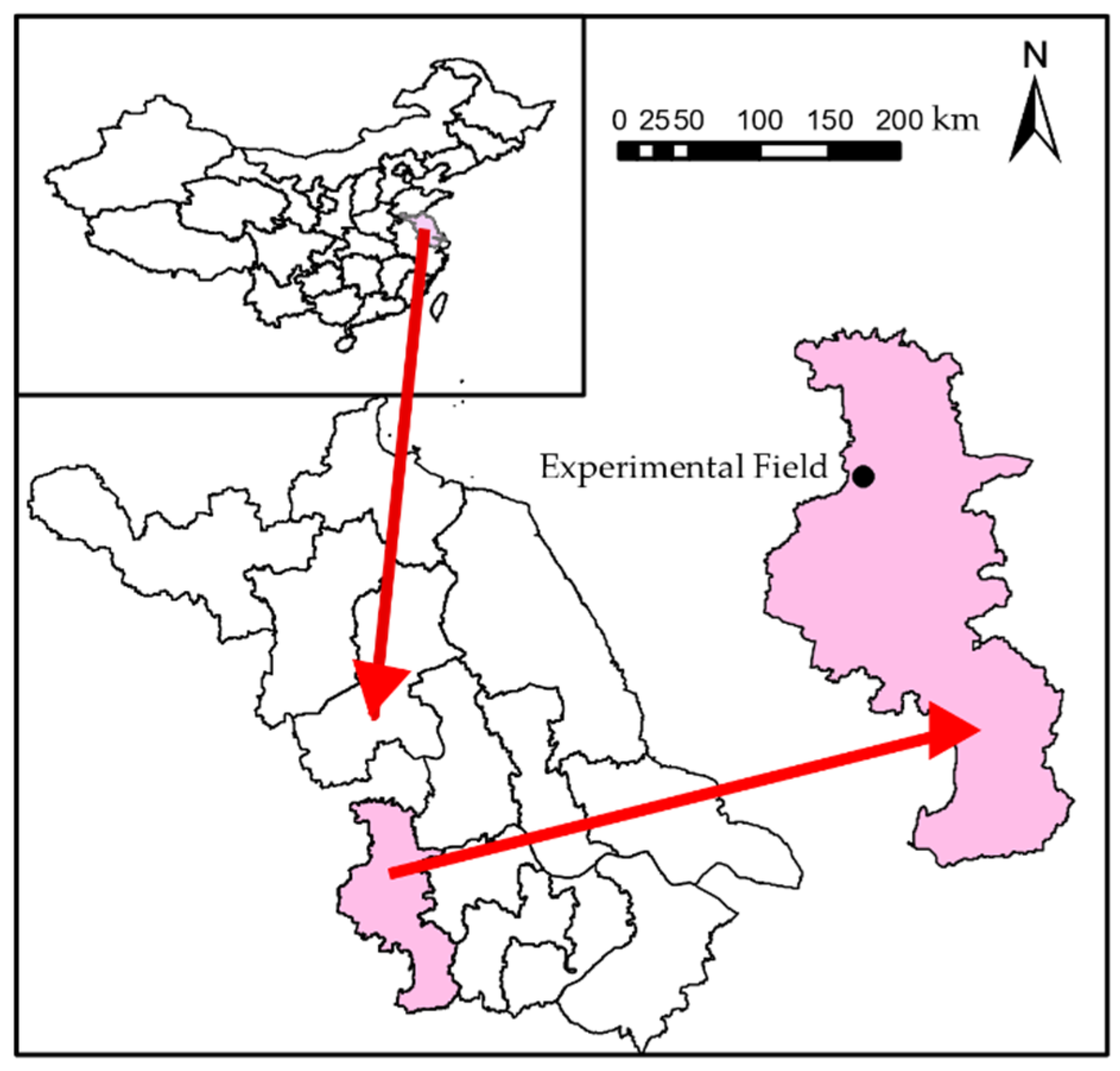
The field experiment was conducted over 3 maize seasons (2016–2018) on the experimental farm of the agro-meteorological station (32.16° N, 118.86° E, Figure 1), which is located in Nanjing, Jiangsu province, China. The region is characterized by a subtropical monsoon humid climate. With obvious seasonal variation of precipitation, it has an average annual rainfall of 1102 mm of which most is received in summer. Characterized with 4 distinctive seasons, it is hot and rainy in summer, and mild and humid in winter. The annual average relative humidity is 76%, and the annual average temperature is 15.4 ℃. More than 200 days in the whole year are frost-free.
The experimental soil was “Magan soil” (mainly distributed in the Jianghuai hilly area and the south bank of the Yangtze River in Jiangsu province, China) [26], which belongs to anthropo-hydrogenic paddy soil. The plough layer is loam clay, which has a clay content of 26.1%, soil bulk density of 1.57 g/cm3 and a soil pH (H2O) value of 6.3. The total carbon and nitrogen contents are 19.95 g/kg and 1.19 g/kg, respectively, and the maize variety was “Jundan 66”. Basic soil characteristics and parameters of the experimental site are shown in Table 1, where it can be seen that all of the characteristics of the soil increased layer-by-layer, but DUL, LL15 and SAT of the soil from the ground surface to the depth of 40 cm have little changes among the 4 soil layers. However, the Airdry changed a lot with the soil layers varied (Table 1).
2.2. Measurements and Variations of Meteorological Factors in Maize Growing Periods
The meteorological data required for 2016–2018 (daily maximum temperature, minimum temperature, precipitation and sunshine hours) were determined by the automatic meteorograph HOBO U30-NCR (Bourne, Onset, MA, USA). The parameters of corn, soil and field management during the crop growth period were derived from the field observations.
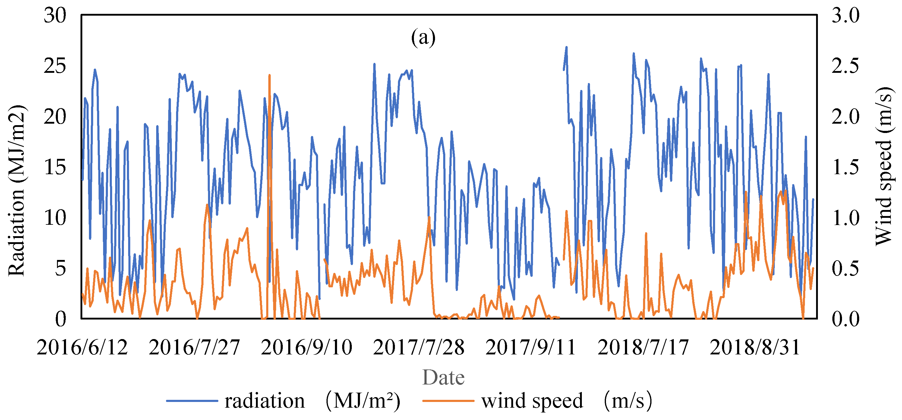
The detailed incoming radiation (Rn), maximum temperature/low temperature, rainfall, wind speed (at 2 m height above the land surface) and relative humidity (RH) in the whole corn growth period are shown in Figure 2a–c, respectively. It is worth noting that as a source of energy for crop evapotranspiration [16], the Rn has the highest correlation coefficient to transpiration among all of the related factors [27]. As shown in Figure 2a, the radiation was relatively large and its value fluctuated obviously during the whole 3 growth periods, with the highest value of 26.82 MJ/m2/d on 15 June 2018, and the lowest value of 1.96 MJ/m2/d on 15 September 2016. In addition, the values on sunny days were larger than those of rainy weather. Meanwhile, the wind speed was basically stable and relatively small during the 3 growth periods, values of it were generally below 1.5 m/s, but its maximum value reached 2.4 m/s, which appeared on 26 August 2016. As can be seen from Figure 2b, during the 3 growth periods, the daily maximum temperature had larger fluctuations annually; however, the daily minimum temperature had larger fluctuations in 2016, and smaller fluctuations in 2017 and 2018. The lowest value was 5.08 °C, which appeared on 21 June 2016, and the highest was 30.12 °C, which appeared on 28 July 2017. In terms of the whole 3 growth periods, the diurnal temperature range in 2016 was relatively larger than that of the other years. As we can see from Figure 2c, the total rainfall in 2016 was less and concentrated in the final days of June and early days of July, and the concentrating period of precipitation in 2017 and 2018 was August. The maximum rainfall reached 182.4 on 15 August 2018, and the secondary peak appeared with a value of 82.7 on 11 July 2018. It can be seen that the annual variation of RH had little change, but its diurnal variation was very large and fluctuated greatly with a highest value of 99.7% and a lowest level of 47.1% during the 3 years. The fluctuation of RH was related to the fluctuation of rainfall and radiation. When the rainfall was large at the beginning and the radiation was low, the relative humidity was relatively large accordingly. Whereas at the end of August and the beginning of September in 2016, the precipitation was basically zero, so the relative humidity was relatively low.
2.3. APSIM Model
Developed by the Australian Agricultural Production Systems Research Group (APSRU), the APSIM (Agricultural Production System Simulator) is an agricultural model to simulate biophysical processes in complex agricultural production systems. In a narrow sense, it is just a mechanism model of systematic agricultural farming. However, a generalized APSIM can simulate systematic processes comprising soil, crop, tree, pasture, grassland and livestock. Being flexible to integrate non-biophysical agricultural resources, such as water storages and agricultural machinery [28], it also contains a series of interconnected biophysical and management models that are used together in simulation analyses. Currently APSIMs have been used in many respects, including horticultural crop system simulation, resource application and its efficiency assessment, climate change and adaptability analysis and analysis of yield variance [29].
The major functional modules can be divided into program management, environment, biology and economy. The management module includes judgment, management and reporting. Some environmental modules include illumination, soil moisture and soil nitrogen. The biological module includes various crops, grasslands and surface residues. All of these modules are interconnected through the “central engine”. Any module can be “plugged in, unplugged”. Among them, the soil module in the environmental module is the core of the APSIM crop model. The Ritchie model is for soil evaporation simulation and the Penman-Monteith water demand is for potential transpiration calculation.
2.3.1. Es Model in APSIM
Applied to calculate Es in the APSIM, the Ritchie model divides the process of evaporation into two stages [30]. The evaporation rate of stage 1 equals the rate of potential evaporation until a specified amount of water has evaporated (U or CONA, the upper limit of evaporate rate in stage 1 cumulative evaporation). The evaporation of soil in stage 2 is a function, which is proportional to the square root of time, and its rate is lower than the rate of potential evaporation. The formulas for stage 1 and 2 are as follows:
where, and are the cumulative values of Es in stage 1 and 2, respectively, t is the total number of Es days after the wetting date, Eso is the amount of potential soil evaporation (replaced with observed evaporation here) each day during stage 1, is the total number of Es days in stage 1, and α (mm/d0.5) is the coefficient in stage 2, and it is assumed to be a constant value for particular soil and mainly depends on soil hydraulic characteristic, ∆ (kPa/°C) is the slope of saturated water vapor pressure, γ (kPa/°C) is the psychrometer constant, Rns (MJ/m2/d) is the average net radiation at the soil surface, Rno (MJ/m2/d) is the average net radiation at canopy, Rs (MJ/m2/d) is the solar radiation, is the albedo for bare soil with a value of 0.1 here [31], is the developing canopy albedo varying with Lai, which is the leaf area index. What is noteworthy is that different soils have different U values. According to the Ritchie experiment, U values of clay, loam and sandy soil are 12 mm, 9 mm and 6 mm, respectively.
2.3.2. Tc Model in APSIM
Based on energy balance and water vapor diffusion, the Tc model in the APSIM is the Penman-Monteith water demand, which is derived from the energy balance equation of crop canopy (evapotranspiration surface). The water demand is caused by two parts: radiation-driven term (PETr) and aerodynamically-driven term (PETa). Tc is the sum of the PETr and PETa. Details are as follows [22,32,33]:
where, N (s) is the day length, Rn (MJ/m2/d) is energy available for evapotranspiration, λ (J/kg) is the latent heat of vaporization, and (kg/m3) represent the density of air and water, D (kPa) is the specific vapor pressure deficit, and Ga and Gc are the (bulk) aerodynamic and surface resistances. Most of the factors can be calculated by the formulas in FAO Irrigation and Drainage Paper No. 56 [34]. In addition, this formula involves the slope of the vapor saturation-temperature curve Δ (kPa/°C), the calculation in the model code are as follows:
where, cp (J/kg) is the specific heat of air at constant temperature, Pair is the air pressure, is the slope of sat. vapor pressure-temperature, T is the average daily temperature, Tabs is 273.16, and esat(T) is the saturated vapor pressure.
2.4. Methods for Parameters Tuning and Model Evaluation
2.4.1. Parameters Calibration of Es
As mentioned earlier, it can be validated that the accuracy of the APSIM simulated Es is mainly related to the CONA value and the α value, therefore we firstly modified the two coefficients with some of the data measured before. In this study, the stage 1 constant CONA (11 mm) was determined from field observations of daily Eo in the early growth periods when Es/Eo remained > 0.9. As mentioned before, “Magan soil” belongs to loam clay, so it can be concluded that the CONA varies from 9 to 12, and trial and error was the first choice. The Eo is calculated as follows [35]:
where, esat (mb) is the saturated vapor pressure at mean air temperature, ea (mb) is the vapor pressure at mean air temperature, Rno (MJ/m2/d) is the average net radiation at canopy (1 mm/d is equivalent to an energy flux of 2.5 MJ/m2/d), and u (km/d) is the wind speed at a height of 2 m.
The stage 2 coefficient was calculated with Equation (2) when the stage 1 was finished in a precipitation process (from a rain occurring to another rain occurring). The α (4.83 mm/d0.5) was the average slope of 4 precipitation cycles in the 2 years.
2.4.2. Determination of Stemflow
Plant stemflow meters can measure the instantaneous runoff density of the plant, which can continuously observe the liquid flow of the plant for a long time, which is conducive to studying the law of water exchange between the plants and the atmosphere. Taking this as an observation means to monitor the impact of the forest ecosystem on environmental changes for a long time, as it has important theoretical guidance significance and application value for afforestation, forest management and forestry management. This study installed the packaged, stem sap flow gauge Flow32A-1K onto the maize stems, which have good growth and no damage in the middle stage of the growth. Before installation, we removed the aging leaves at the bottom of the corn, and the sensors were installed at the stem base of the corn, approximately 10 cm from the soil surface, to monitor the stemflow velocity of plants so as to test the simulation results. In order to prevent the sensors’ damage by water absorption of external wrapped foam and avoid the measuring error caused by the growth of maize adventitious root, the sensors were removed after heavy rain, and installed back to the original positions after they dried.
2.4.3. Methods of Model Evaluation
The performance of the crop models is often evaluated by using linear regression by least squares. However, the coefficient of determination (R2) alone, in general, is often inappropriate and has deficiencies when used to compare predicted and observed values. Therefore, an index of agreement (D), as well as the systematic root mean square error (RMSEs) and unsystematic error (RMSEu), were suggested to use for comparisons of model-predicted and observed variables [36,37,38,39].
where, the coefficient R2 and D, ranged from 0 to 1, represents the consistency between the simulated and measured values. The closer that the value is to 1, the higher the fitting degree is. Herein, Xi and Yi are measured and simulated values, respectively, and are the average of measured and simulated values, respectively, is the regression estimate for the observation, and n is the number of observations. The smaller the RMSE value is, the better the fitting effect.
3. Results
3.1. Simulated and Observed Es from Maize
3.1.1. Es Variation in the Maize Growth Periods
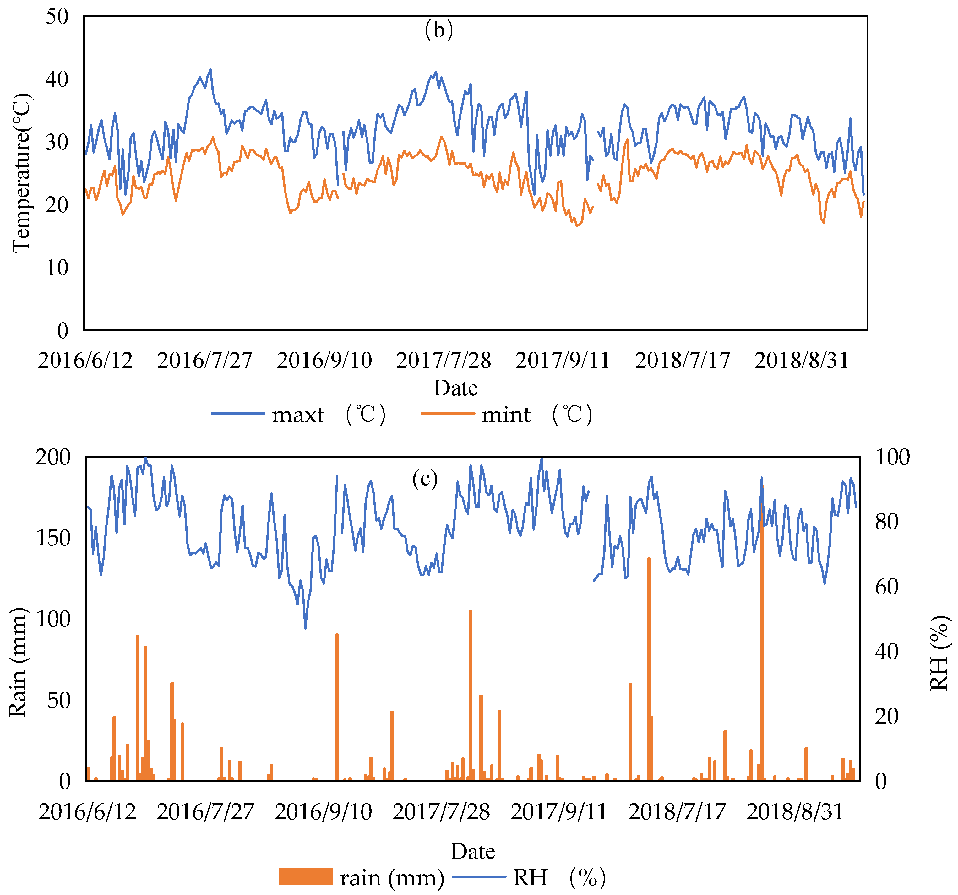
As shown in Figure 3, the simulated and observed Es both in 2016 and 2017 fluctuated greatly and remained at a high level in early growth periods and gradually declined with fluctuation during the late stages of growth. In addition, it was lower with a stable tendency separately during the late stages of maize development. The variation trends of the simulated Es both in the two years were broadly in line with the observed values. In addition, the highest simulated Es in 2016 was 5.74 mm/d and appeared on 26 June, and the lowest one was 0.16 mm/d, which appeared on 14 July. The highest observed Es in 2016 was 5.95 mm/d and occurred on 26 June, and the lowest one was 0.24 mm/d, which appeared on 14 September. In 2017, the simulated Es reached a peak of 4.42 mm/d on 23 June, and reached the valley value of 0.08 mm on 4 September. The observed Es peaked on 10 July at 3.91mm/d, and touched bottom on 21 August at 0.10 mm/d. In general, the Es in 2016 was higher than in 2017. It should be noted that there are some missing observed data because we did not have the means to collect data on rainy or other bad weather days, and the data collection started after maize emergence in 2017.
3.1.2. Comparison of Simulated and Observed Es
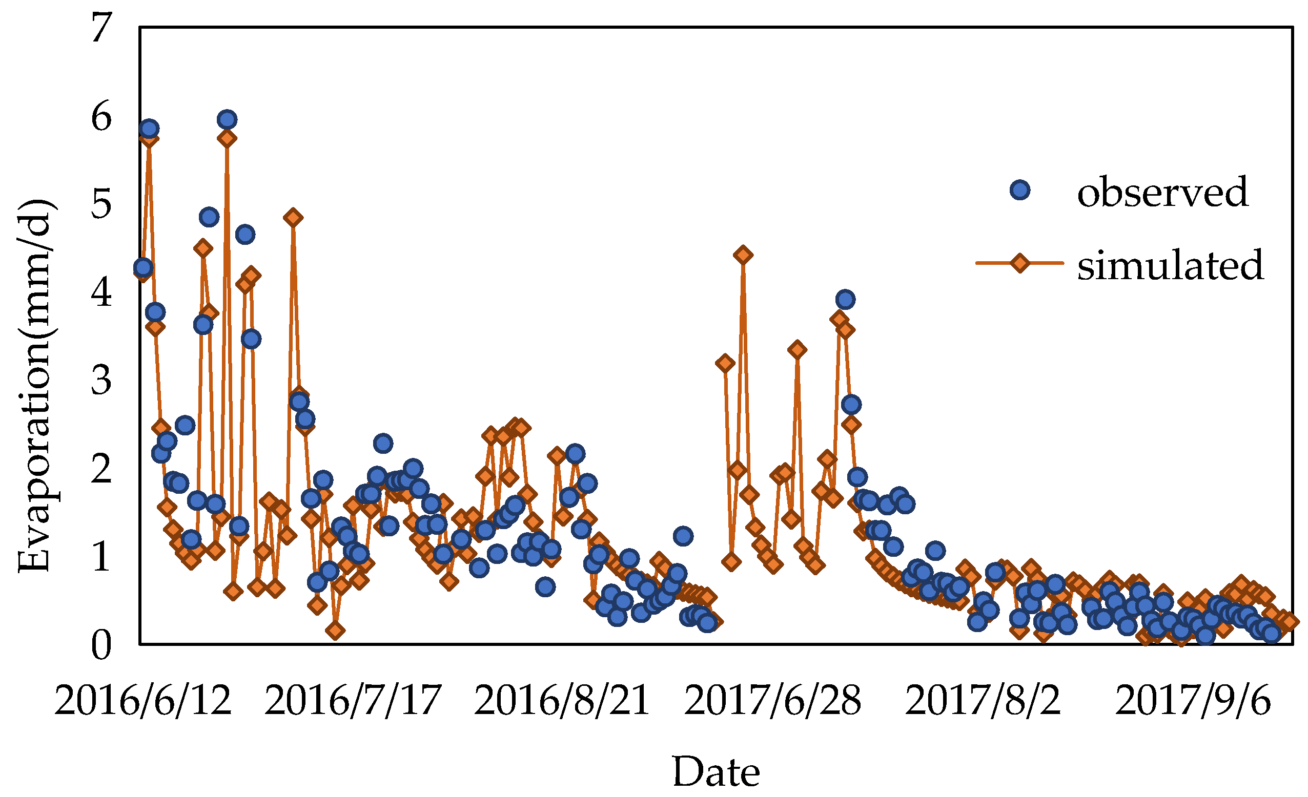
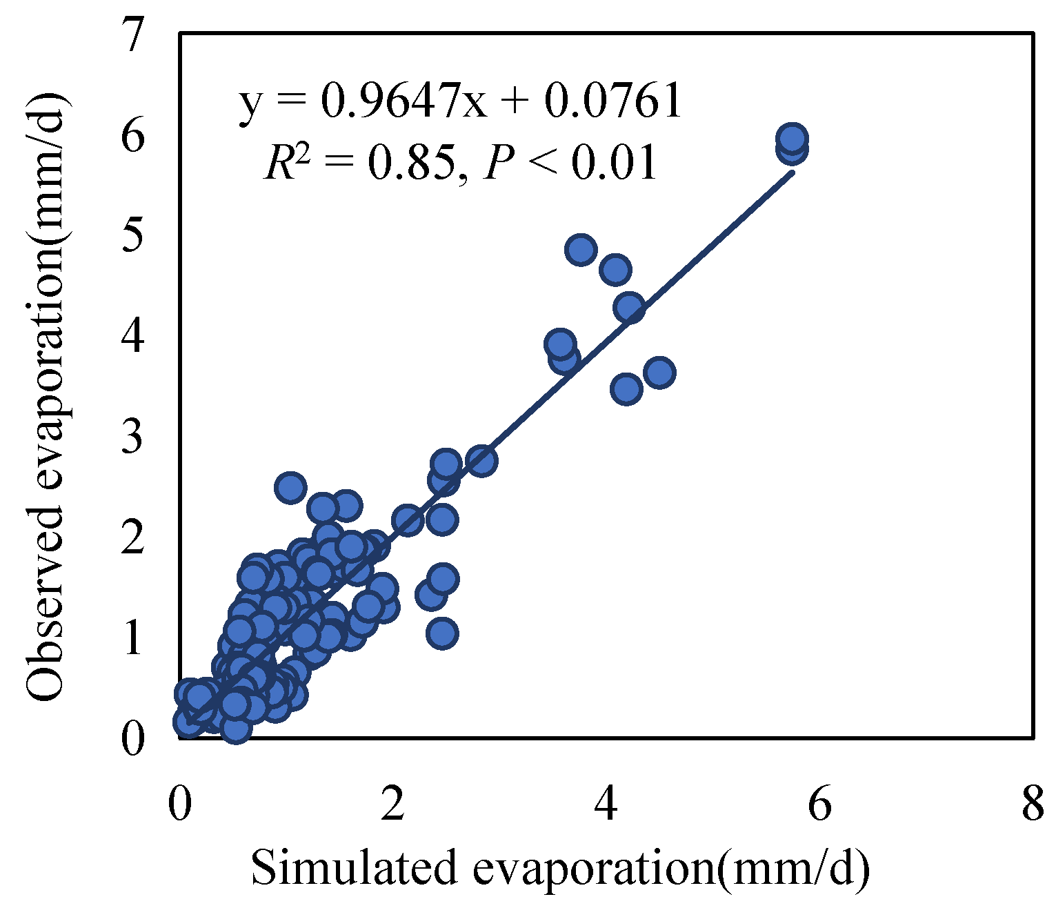
It can be seen that the APSIM-simulated and the field-measured values had the same trends both in the 2016 and 2017 maize growth periods. The determination coefficient R2 = 0.85 (p < 0.01), the adjusted determination coefficient R2 = 0.85 and the index of agreement D = 0.96 (Figure 4, Table 2), which means the relationship between the simulated and the measured values reaches an extremely significant level. The RMSEs = 0.0783 mm/d, RMSEu = 0.4435 mm/d (Table 2), and the fitted slope was 0.9647 (Figure 4), which means the ratio of the simulated value to the measured value was close to 1:1 and the model had a small regression error. The variation curves of the simulated value in the two years were basically consistent with the responsive measured values, except that the simulated value was obviously higher than the measured value in August 2016 (Figure 3). The Es was in stage 2, and the simulated values were the potential evaporation; however, the soil moisture was not sufficient to support theoretical amounts for there was little rain during this period. Individually, the fitting degree in 2016 (R2 = 0.81) was better than that in 2017 (R2 = 0.80), and yet there was no remarkable difference between the two. However, compared with the total fitting degree, both the two fitting degrees in 2016 and 2017 were significantly lower than the total one.
3.2. Simulated and Observed Tc from Maize
3.2.1. Tc Variation in the Maize Growth Periods
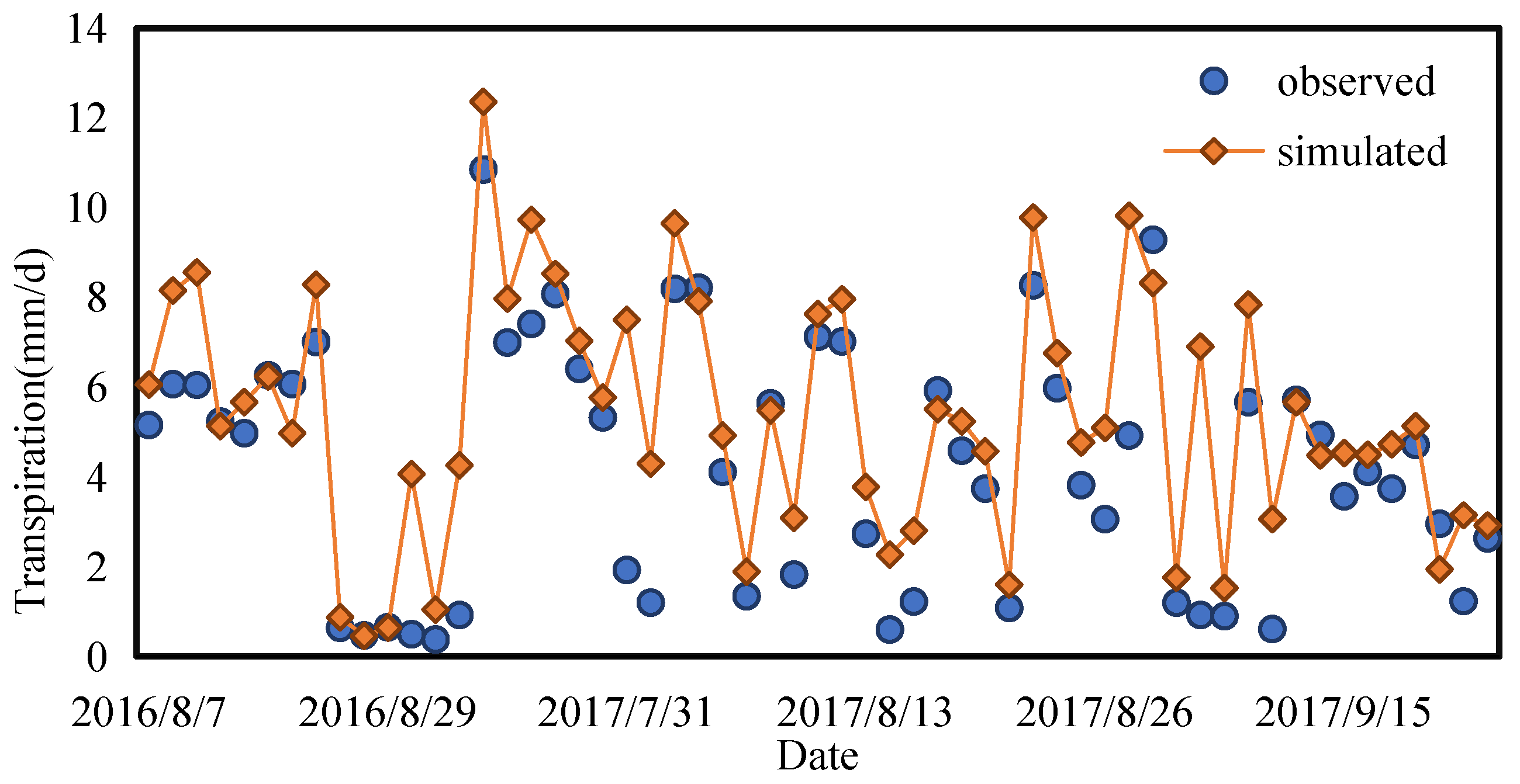
As shown in Figure 5, the simulated Tc both in 2016 and 2017 fluctuated greatly. It was lower in early growth periods, then rose rapidly and remained at a high level in middle growth periods and gradually declined with fluctuation during the late stages of growth. The installation of equipment was in the middle periods of the crop growth, and equipment should be dismantled on rainy days. However, even without enough time to disassemble the equipment on occasion, the maintenance and repair must be undertaken a long time after raining. Therefore, there was no complete observed data, but it showed that the simulated Tc values were basically consistent with the observed values. In 2016, the simulated Tc reached a peak of 12.15 mm/d on 24 July. In 2017, the highest simulated value was 13.07 mm/d and appeared on 19 July. The simulated Tc in 2016 was higher than in 2017 on the whole.
3.2.2. Comparison of Simulated and Observed Tc
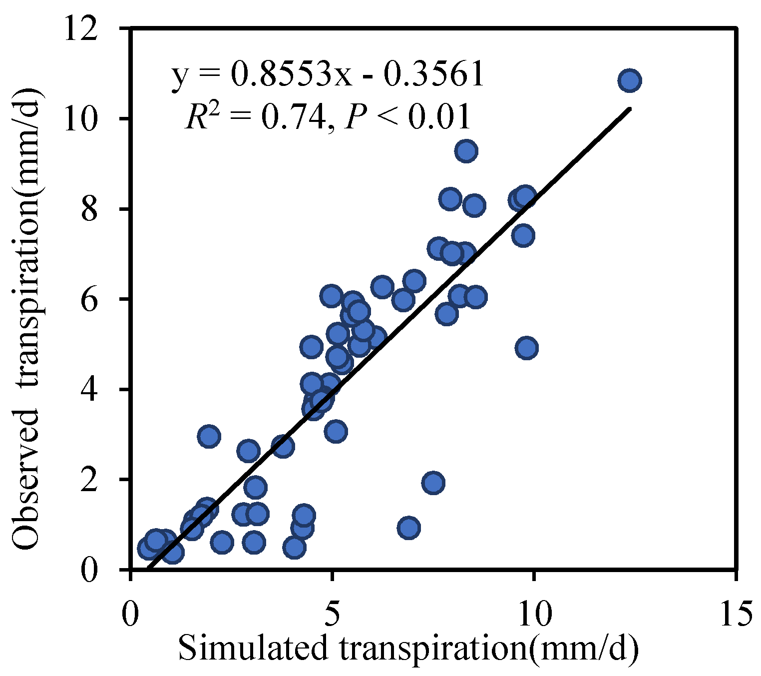
From Figure 6, it can be seen that there was a correlation between the simulated and observed Tc values. However, the fitting degree between the simulated and observed Tc was not very good, which was reflected in the determination coefficient R2 = 0.74 (p < 0.001) (Figure 6). The RMSEs = 1.2261 mm/d and the RMSEu = 1.4197 mm/d (Table 2) means that the predicted ratings slightly deviated from the true ones. However, the simulated and observed Tc had good agreement, connoted by the index agreement D = 0.82. and the fitted slope was 0.8553 (Figure 6), all of which meant that the fitting degree between the simulated and observed Tc was not “high” but statistically significant. Compared with the observed Tc, it was shown that the trends of fluctuation in the two growth periods of 2016 and 2017 were basically consistent (Figure 6). The fluctuation frequencies of the simulated Tc were basically consistent with the observed, but the values of the simulated Tc were higher than the observed.
4. Discussions
As global warming has intensified, the contradiction between the water supply and demand has become increasingly obvious. Accurate predictions of Es and Tc have become increasingly important, since both of them are of great importance in water balance calculation. The APSIM water balance model can simulate the Es and presented good adaptability in Nanjing area, the same as in Southwestern, Ningxia, Gansu and Northeast of China [24,36,40,41]. However, different areas have different fitting degrees. Ma et al. [42] showed that the simulated and measured soil moisture content have a significant positive correlation (the value of R2 was between 0.959~0.973). Li et al. [43] showed that the relationship was found between predicted and observed soil storage water (R > 0.7) with a variation of ±20%. As inferred, the method of model parameter optimization and experimental observations in different tests are different, which could affect the results and fitting degrees. The validation water balance process of the APSIM model gives a convenient method to simulate the Es and Tc by crop growing models. After calibrating the parameters needed in the simulation, the water consumption of the maize field would be predicted under both climate change and crop growth variation. Moreover, the APSIM helps simulate the production of the maize field.
The simulation of Tc in the APSIM uses the Penman-Monteith water demand. With improved Penman-Monteith, most researchers showed good fitting results. Lu (2008) showed that the error between the simulated and the measured Tc was −1.2% [44], and Gao et al. [45] showed that the simulated and the observed values fit well (R2 = 0.70). Moreover, Li et al. and Yan et al. [46,47] demonstrated that the simulated and measured values of Tc had good agreement. In similarity with the above, the result of the simulated Tc in this paper was also good (R2 = 0.74). The reason may be the APSIM model separated ET into Es and Tc, which improves the Es and Tc simulation, respectively. In addition, it is worthless that there are not unified standards for the calculation of some parameters needed in the Penman-Monteith. Different formulas for parameters calculation may influence the estimation values. As well, the Penman-Monteith neglected the energy consumption of inner dissipation and photosynthesis and did not take the airflow exchange and the atmospheric stratification into account [32]. Moreover, the Penman-Monteith water demand in the APSIM amplifies the effects of the VPD (vapor pressure deficit), which may lead to errors. Therefore, the applicability of the Penman-Monteith model and the method of parameters determination are still controversial [48].
5. Conclusions
In order to evaluate the performance and the adaptability of evaporation and transpiration simulating by the APSIM in a humid area in Nanjing, China, this paper compares two simulations of Es and Tc by APSIM with the measured Es and Tc. Analysis over the study area revealed that the systematic root mean square error RMSEs and unsystematic root mean square error RMSEu of Es were 0.08 and 0.44 mm/d, respectively. The determination coefficient R2 and adjusted R2 was 0.85, (p < 0.001) and the index agreement D was 0.96, which connoted that the correlation degree reached a significant level. Based on the results, it was concluded that the calibrated Ritchie model in the APSIM can simulate the Es during maize growth periods in Nanjing. From the results that the RMSEs and RMSEu were 1.22 and 1.42 mm/d, respectively, the R2 was 0.74 and the index agreement D was 0.88 in the simulation of Tc, it can be concluded that compared with the Es simulation, the Tc simulation error of the APSIM should be further reduced and the performance of the model should be further improved in Nanjing. However, it also has a good agreement with the observed values. The results of this project may be beneficial to further research on field moisture. Both of the Es and Tc simulations can provide a reference for water-saving irrigation.
Author Contributions
Conceptualization, T.G. and C.L.; methodology, T.G.; software, T.G.; validation, T.G., Y.X. and P.Z.; formal analysis, T.G.; data curation, C.L. and R.W.; writing—original draft preparation, T.G.; writing—review and editing, Y.X., C.L. and R.W. All authors have read and agreed to the published version of the manuscript.
Funding
This research received no external funding.
Institutional Review Board Statement
Not applicable.
Informed Consent Statement
Not applicable.
Data Availability Statement
The study did not report any data.
Acknowledgments
We are grateful for grants from the national key research and development plan (2019YFC0507403) and Jiangsu Key Laboratory Program of Aro-meteorology from Nanjing University of Information Science and technology (JKLAM1703).
Conflicts of Interest
The authors declare no conflict of interest.
References
- Li, F.X.; Ma, Y.J. Evapotranspiration Estimation of Summer Maize with Plastic Mulched Drip Irrigation Based on Dual Crop Coefficient Approach in Xinjiang. Trans. Chin. Soc. Agric. Mach. 2018, 49, 268–274. [Google Scholar]
- Wang, J.; Wang, J.L.; Liu, J.B.; Jiang, W.; ZHao, C.X. Parameters modification and evaluation of two evapotranspiration models based on Penman-Monteith model for summer maize. Chin. J. Appl. Ecol. 2017, 28, 1917–1924. [Google Scholar]
- Qiu, R.J.; Katul, G.G.; Wang, J.T.; Xu, J.Z.; Kang, S.D.; Liu, C.W.; Zhang, B.Z.; Li, L.A.; Cajucom, P.E. Differential response of rice evapotranspiration to varying patterns of warming. Agric. For. Meteorol. 2021, 298–299, 108293. [Google Scholar] [CrossRef]
- Dhillon, R.; Rojo, F.; Upadhyaya, S.K.; Roach, J.; Delwiche, M. Prediction of plant water status in almond and walnut trees using a continuous leaf monitoring system. Precis. Agric. 2019, 20, 723–745. [Google Scholar] [CrossRef]
- Balwinder-Singh; Eberbach, P.L.; Humphreys, E. Simulation of the evaporation of soil water beneath a wheat crop canopy. Agric. Water Manag. 2014, 135, 19–26. [Google Scholar] [CrossRef]
- Leuning, R.; Condon, A.G.; Dunin, F.X.; Zegelin, S.; Denmead, O.T. Rainfall inter ception and evaporation from soil below a wheat canopy. Agric. For. Meteorol. 1994, 67, 221–238. [Google Scholar] [CrossRef]
- Boast, C.; Robertson, T. A “micro-lysimeter” method for determining evaporation from bare soil: Description and laboratory evaluation. Soil Sci. Soc. Am. J. 1982, 46, 689–696. [Google Scholar] [CrossRef]
- Kool, D.; Agam, N.; Lazarovitch, N.; Heitman, J.; Sauer, T.; Ben-Gal, A.J. A review of approaches for evapotranspiration partitioning. Agric. For. Meteorol. 2014, 184, 56–70. [Google Scholar] [CrossRef]
- Gao, X.F.; Shi, H.Z.; Yang, J.; Wang, X.L. Advances in soil evaporation measured by micro-lysimeter. Adv. Sci. Technol. Water Resour. 2010, 30. [Google Scholar] [CrossRef]
- Allen, S.J. Measurement and Estimation of Evaporation from Soil under Sparse Barley Crops in Northern Syria. Agric. For. Meteorol. 1990, 49, 291–309. [Google Scholar] [CrossRef]
- Liu, X.F.; Sun, J.S.; Liu, Z.G.; Wang, S.S.; Wang, J.L.; NaTian, C. Soil Evaporation of Summer Corn under Alternate-furrow Irrigation Condition. Water Sav. Irrig. 2007, 6, 10–12. [Google Scholar]
- Moran, M.; Scott, R.; Keefer, T.; Emmerich, W.; Hernandez, M.; Nearing, G.; Paige, G.; Cosh, M.; O’Neill, P. Partitioning evapotranspiration in semiarid grassland and shrubland ecosystems using time series of soil surface temperature. Agric. For. Meteorol. 2009, 149, 59–72. [Google Scholar] [CrossRef]
- Liu, Y.T. Evaporation Test and Model Study of Saline-Alkalne Soil. Master’s Thesis, Xi’an University of Technology, Xi’an, China, 2019. [Google Scholar]
- Ma, L.; Wei, G.H. Fitness-for-service of evaporatranspiration model in Tarim Basin, Xinjing. J. Arid. Land Resour. Environ. 2015, 29, 132–137. [Google Scholar]
- Tan, G.Y. The Application of APSIM Model and the Measurement of Soil Evaporation Parameters in the Qingyang Loess Plateau, Gansu. Master’s Thesis, Lanzhou University, Lanzhou, China, 2007. [Google Scholar]
- Didari, S.; Ahmadi, S.H. Calibration and evaluation of the FAO56-Penman-Monteith, FAO24-radiation, and Priestly-Taylor reference evapotranspiration models using the spatially measured solar radiation across a large arid and semi-arid area in southern Iran. Theor. Appl. Climatol. 2019, 136, 441–455. [Google Scholar] [CrossRef]
- Li, Q.; Jing, Y.S.; Li, K. Comparation of rice field evaporatranspiration models in two time scales. Jiangsu Agric. Sci. 2019, 47, 238–243. [Google Scholar]
- Mi, N.; Chen, P.S.; Zhang, Y.S.; Ji, R.P.; Zhou, G.S.; Li, R.P. Applications and Comparations of evaportranspiration models in maize field. Resour. Sci. 2009, 31, 1599–1606. [Google Scholar]
- Zheng, Z.; Cai, H.J.; Yu, L.Y.; Wang, J. Comparison of Two Crop Evapotranspiration Calculating Approaches in CSM-CERES-Wheat Model. Trans. Chin. Soc. Agric. Mach. 2016, 47, 179–191. [Google Scholar] [CrossRef]
- Qiu, R.; Liu, C.; Cui, N.; Wu, Y.; Wang, Z.; Li, G. Evapotranspiration estimation using a modified Priestley-Taylor model in a rice-wheat rotation system. Agric. Water Manag. 2019, 224, 105755. [Google Scholar] [CrossRef]
- Qiu, R.; Du, T.; Wu, L.; Chen, R.; Kang, S. Assessing the SIMDualKc model for estimating evapotranspiration of hot pepper grown in a solar greenhouse in Northwest China. Agric. Syst. 2015, 138, 1–9. [Google Scholar] [CrossRef]
- Snow, V.; Huth, N. The APSIM-MICROMET Module; HortResearch: Auckland, New Zealand, 2004; pp. 1–18. [Google Scholar]
- Zhang, J.H.; Wag, X.Y.; Zhou, D.M.; Wang, G.Y. Simulation on water-saving optimization irrigation schedule of winter wheat-summer maize double cropping system in Haihe Plain. J. Hebei Agric. Univ. 2018, 41, 24–30. [Google Scholar] [CrossRef]
- Dai, T.; Wang, J.; He, D.; Wang, N. Modeling the impacts of climate change on spring maize yield in Southwest China using the APSIM model. Resour. Sci. 2016, 38, 155–165. [Google Scholar] [CrossRef]
- Ru, X.Y.; Li, G.; Yan, L.J.; Chen, G.P.; Nie, Z.G. Effect of precipitation and nitrogen application on spring wheat yield in dryland based on APSIM model. Pratacultural Sci. 2019, 36, 2342–2350. [Google Scholar] [CrossRef]
- Li, L. Analysis of Evolutionary Law and Control Measures of Magan Soil. J. Anhui Agric. Sci. 1964, 29–36. (In Chinese) [Google Scholar] [CrossRef]
- Liu, C.; Wu, X.; QIU, R. Evaluation of Evapotranspiration of Maize With Crop Coefficient and Penman-Monteith Methods in Nanjing. Water Sav. Irrig. 2016, 09, 12–17. [Google Scholar]
- Holzworth, D.; Huth, N.I.; Fainges, J.; Brown, H.; Zurcher, E.; Cichota, R.; Verrall, S.; Herrmann, N.I.; Zheng, B.; Snow, V. APSIM Next Generation: Overcoming challenges in modernising a farming systems model. Environ. Model. Softw. 2018, 103, 43–51. [Google Scholar] [CrossRef]
- Carberry, P.S.; Liang, W.-L.; Twomlow, S.; Holzworth, D.P.; Dimes, J.P.; McClelland, T.; Huth, N.I.; Chen, F.; Hochman, Z.; Keating, B.A. Scope for improved eco-efficiency varies among diverse cropping systems. Proc. Natl. Acad. Sci. USA 2013, 110, 8381–8386. [Google Scholar] [CrossRef] [Green Version]
- Ritchie, J.T. Model for predicting evaporation from a row crop with incomplete cover. Water Resour. Res. 1972, 8, 1204–1213. [Google Scholar] [CrossRef] [Green Version]
- Gao, Y.; Duan, A.W.; Chen, J.P.; Shen, X.J.; Liu, Z.D. Modeling soil evaporation in maize/soybean strip intercropping systems. In Proceedings of the Fifth National Conference Collected Paper of Chinese Society of Agricultural Engineering Agricultural Water Soil Energeering, Shihezi, China, 1 July 2008; pp. 87–91. [Google Scholar]
- Kang, S.Z.; Xiong, Y.Z.; Liu, X.M. A Study of Penman-Monteith model to estimate transpiration from crops. J. Northwest A F Univ. 1991, 19, 13–20. [Google Scholar]
- Sun, J.S.; Chen, Y.M.; Kang, S.Z.; Xiong, Y.Z. Study on estimation of crop transpiration and soil evaporation in summer corn field. J. Maize Sci. 1996, 4, 76–80. [Google Scholar] [CrossRef]
- Allen, R.G.; Pereira, L.S.; Raes, D.; Smith, M. FAO Irrigation and drainage paper. Rome Food Agric. Organ. United Nations 1998, 56, e156. [Google Scholar]
- Penman, H.L. Vegetation and hydrology. Soil Sci. 1963, 96, 357. [Google Scholar] [CrossRef]
- Ao, H.W.; Xie, Y.Z.; Li, Y.H.; Ma, J.L. Adaptability of APSIM Model in Simulating Lucerne-Wheat-Millet Crop Rotation System in Haiyuan Region of Ningxia. Acta Agrestia Sin. 2016, 24, 146–155. [Google Scholar]
- Inman-Bamber, N.; Jackson, P.; Stokes, C.; Verrall, S.; Lakshmanan, P.; Basnayake, J. Sugarcane for water-limited environments: Enhanced capability of the APSIM sugarcane model for assessing traits for transpiration efficiency and root water supply. Field Crop. Res. 2016, 196, 112–123. [Google Scholar] [CrossRef]
- Willmott, C.J. Some comments on the evaluation of model performance. Bull. Am. Meteorol. Soc. 1982, 63, 1309–1313. [Google Scholar] [CrossRef] [Green Version]
- Willmott, C.J. On the validation of models. Phys. Geogr. 1981, 2, 184–194. [Google Scholar] [CrossRef]
- Liu, Z.J.; Yang, X.G.; Wang, J.; LV, S.; LI, K.N.; Xun, X.; Wang, E.L. Adaptability of APSIM Maize Model in Northeast China. Acta Agron. Sin. 2012, 38, 740–746. [Google Scholar] [CrossRef]
- Yang, X.; YangTan, G.; Shen, Y.Y. Soil Moisture Content under Stubble Retention After Dry framing Winter Wheat Harvest Based on APSIM Model. Arid. Zone Res. 2013, 30, 609–614. [Google Scholar]
- Ma, C.Q.; Li, G.; Wang, J.; Ru, X.Y. Effect of farming practices on spring wheat yield by using APSIM model. Trop. Agric. Eng. 2020, 44, 67–71. [Google Scholar]
- Li, G.; Huang, G.B.; Bellotti, W.; Chen, W. Adaptation Research of APSIM Model under Different Tillage Systems in the Loess hill-gullied Region. Acta Ecol. Sin. 2009, 29, 2655–2663. [Google Scholar]
- Lu, X.J. Studies on the Methods of Utilizing Penman-Monteith Equation to Calculate Evapotranspiration of Forest. Master’s Thesis, Beijing Forestry University, Beijing, China, 2008. [Google Scholar]
- Gao, Z.Q.; Li, T.; Zhang, X.C. Dynamic simulation of canopy transpiration in apple tree. J. Fruit Sci. 2009, 26, 775–780. [Google Scholar]
- Li, L.; Dong, X.H.; Zhao, Q.; Fang, Y.; Yao, Z.X.; Su, H. Observation and Simulation of the Outdoors Evapotranspiration for Citrus Trees. J. Irrig. Drain. 2016, 35, 98–104. [Google Scholar]
- Yan, H.F.; Zhao, B.S.; Zhang, C.; Huang, S.; Fu, H.; Yu, J.J.; Acquah, S.J. Estimating cucumber plants transpiration by Penman-Monteith model in Venlo-type greenhouse. Trans. Chin. Soc. Agric. Eng. 2019, 35, 149–157. [Google Scholar]
- Zhang, B.; Xu, D.; Liu, Y.; Chen, H. Review of multi-scale evapotranspiration estimation and spatio-temporal scale expansion. Trans. Chin. Soc. Agric. Eng. 2015, 31, 8–16. [Google Scholar] [CrossRef]
Figure 1.
Location of experimental farm in Nanjing, Jiangsu province of China.

Figure 2.
Radiation and wind speed (a), maximum/low temperatures (b), rain and relative humidity (RH) (c) during maize growth during 2016–2018.
Figure 2.
Radiation and wind speed (a), maximum/low temperatures (b), rain and relative humidity (RH) (c) during maize growth during 2016–2018.


Figure 3.
Comparison of APSIM simulated and field observed daily evaporation in 2016 and 2017. The observed data was obtained by weighing micro-lysimeter every day, and calculating differences between two successive days.
Figure 3.
Comparison of APSIM simulated and field observed daily evaporation in 2016 and 2017. The observed data was obtained by weighing micro-lysimeter every day, and calculating differences between two successive days.

Figure 4.
The linear regression between simulated and observed evaporation values during maize growth in 2016 and 2017.
Figure 4.
The linear regression between simulated and observed evaporation values during maize growth in 2016 and 2017.

Figure 5.
Comparison of simulated and observed crop transpiration in 2016 and 2017.

Figure 6.
The linear regression between simulated and observed transpiration values during partial maize growth in 2016 and 2017.
Figure 6.
The linear regression between simulated and observed transpiration values during partial maize growth in 2016 and 2017.


Table 1.
Soil hydraulic characteristics of experimental site.
| Soil Depth (cm) | Air Dry (mm/mm) | DUL (mm/mm) | LL15 (mm/mm) | SAT (mm/mm) |
|---|---|---|---|---|
| 0~5 | 0.038 | 0.221 | 0/119 | 0.300 |
| 5~15 | 0.136 | 0.250 | 0.136 | 0.300 |
| 15~25 | 0.150 | 0.268 | 0.160 | 0.322 |
| 25~40 | 0.158 | 0.274 | 0.167 | 0.311 |
Notes: Air dry: air dry for each soil layer; DUL: drainage upper limit (0.33 bar) for each soil layer; LL15: lower limit (15 bar) for each soil layer; SAT: saturation (0 bar) for each soil layer.
Table 2.
Regression statistics for simulated versus observed Es and Tc both in 2016 and 2017.
| Sub-Models | R2 | D | p-Value | RMSEs (mm/d) | RMSEu (mm/d) |
|---|---|---|---|---|---|
| Es | 0.85 | 0.96 | 0.000 | 0.0783 | 0.4435 |
| Tc | 0.74 | 0.88 | 0.000 | 1.2261 | 1.4197 |
Publisher’s Note: MDPI stays neutral with regard to jurisdictional claims in published maps and institutional affiliations. |
© 2021 by the authors. Licensee MDPI, Basel, Switzerland. This article is an open access article distributed under the terms and conditions of the Creative Commons Attribution (CC BY) license (https://creativecommons.org/licenses/by/4.0/).
Share and Cite
MDPI and ACS Style
Guo, T.; Liu, C.; Xiang, Y.; Zhang, P.; Wang, R. Simulations of the Soil Evaporation and Crop Transpiration Beneath a Maize Crop Canopy in a Humid Area. Water 2021, 13, 1975. https://doi.org/10.3390/w13141975
AMA Style
Guo T, Liu C, Xiang Y, Zhang P, Wang R. Simulations of the Soil Evaporation and Crop Transpiration Beneath a Maize Crop Canopy in a Humid Area. Water. 2021; 13(14):1975. https://doi.org/10.3390/w13141975
Chicago/Turabian StyleGuo, Tianting, Chunwei Liu, Ying Xiang, Pei Zhang, and Ranghui Wang. 2021. "Simulations of the Soil Evaporation and Crop Transpiration Beneath a Maize Crop Canopy in a Humid Area" Water 13, no. 14: 1975. https://doi.org/10.3390/w13141975
Note that from the first issue of 2016, this journal uses article numbers instead of page numbers. See further details here.