
Simulating Diurnal Variations of Water Temperature and Dissolved Oxygen in Shallow Minnesota Lakes


1
Department of Civil and Environmental Engineering, Auburn University, Auburn, AL 36849, USA
2
Connecticut Department of Transportation, Newington, CT 06111, USA
3
Key Laboratory of Mariculture, Ministry of Education, Ocean University of China, Qingdao 266100, China
*
Author to whom correspondence should be addressed.
Water 2021, 13(14), 1980; https://doi.org/10.3390/w13141980
Submission received: 1 June 2021
/
Revised: 4 July 2021
/
Accepted: 15 July 2021
/
Published: 19 July 2021
(This article belongs to the Special Issue Physical Processes in Lakes)
Abstract
:In shallow lakes, water quality is mostly affected by weather conditions and some ecological processes which vary throughout the day. To understand and model diurnal-nocturnal variations, a deterministic, one-dimensional hourly lake water quality model MINLAKE2018 was modified from daily MINLAKE2012, and applied to five shallow lakes in Minnesota to simulate water temperature and dissolved oxygen (DO) over multiple years. A maximum diurnal water temperature variation of 11.40 °C and DO variation of 5.63 mg/L were simulated. The root-mean-square errors (RMSEs) of simulated hourly surface temperatures in five lakes range from 1.19 to 1.95 °C when compared with hourly data over 4–8 years. The RMSEs of temperature and DO simulations from MINLAKE2018 decreased by 17.3% and 18.2%, respectively, and Nash-Sutcliffe efficiency increased by 10.3% and 66.7%, respectively; indicating the hourly model performs better in comparison to daily MINLAKE2012. The hourly model uses variable hourly wind speeds to determine the turbulent diffusion coefficient in the epilimnion and produces more hours of temperature and DO stratification including stratification that lasted several hours on some of the days. The hourly model includes direct solar radiation heating to the bottom sediment that decreases magnitude of heat flux from or to the sediment.
1. Introduction
Water quality of natural water systems is of great concern in the modern world because of the importance of water in human life and the environment. Water temperature and dissolved oxygen (DO) are the two most important water quality parameters for aquatic systems since temperature affects DO and the availability of DO in lakes affects freshwater fish species and populations [1]. In the later part of the twentieth century, due to the advent of modern computers, various numerical models have been developed to predict water quality parameters in different types of waterbodies such as riverine systems, estuaries, lakes, and reservoirs. Most of the time, lakes are simulated using one-dimensional models that assume well mixed or uniform conditions along horizontal layers and only recognize major variations in water quality along the vertical (depth) direction. The assumption with one-dimensional models is that all inflow quantities and constituents are instantaneously dispersed throughout the horizontal layers [2]. The turbulent diffusion approach and the mixed-layer approach [3] are the two approaches commonly used to model water temperature and DO in a lake. There are quite a number of water quality models for simulating the water quality of a lake. Almost all the models developed previously have one common characteristic: they are all based on a daily time step. In this study, a deterministic one-dimensional year-round daily water quality model—MINLAKE2012 [4] was modified to capture the hourly fluctuations of water quality parameters in shallow lakes (named MINLAKE2018).
The Minnesota Lake Water Quality Management Model (MINLAKE) is a deterministic one-dimensional model with a time step of one day that was developed in the 1980s for lake eutrophication studies and control strategies [5]. When the model was developed, the lack of temporal data did not allow the development of a diurnal-nocturnal model with a shorter time step, e.g., one hour. Since horizontal variations of water temperature and DO in freshwater lakes are relatively small compared to vertical variations, the one-dimensionality of MINLAKE is appropriate for freshwater lakes. The model has been successfully applied to many lakes over several years with satisfactory results [6,7,8]. To provide decision-makers with a useful tool for lake management and restoration, the MINLAKE model has been frequently reviewed, modified, and updated to improve accuracy and confidence. For example, a regional MINLAKE model was developed in the early 1990s and comprised of two separate sub-models—a regional water temperature model [9] and a regional dissolved oxygen model [10]. Though MINLAKE models were originally developed to simulate water quality during periods of open water it was observed that heat and oxygen transfer processes through the open water surface were substantially altered by winter ice and snow cover [11]. As a result, separate sub-models were developed for winter conditions and integrated with MINLAKE to provide the capability to simulate year-round water temperature and DO, and the revised model is called MINLAKE96. To account for water-sediment heat exchange, a separate sub-model, which calculates temperature profiles in the sediment below the water-sediment interface, was developed [12]. Fang and Stefan [12] found that heat fluxes between lake water and sediment could be substantial. Both simulated and field measurements have shown that shallow lakes can become 1–2 °C warmer under a thick winter ice/snow cover without significant radiation penetration through the snow/ice-covered surface, or significant flow into and out of a lake [13]. The year-round water temperature simulation model has been expanded significantly by simulating the winter ice and snow cover and including heat exchange between water layers and sediment [14]. Moreover, the model was further refined for coefficients used to accurately project water quality in deep cisco lakes, resulting in the MINLAKE2012 model. This is the version of the MINLAKE model used in our study.
Xu and Xu [15] revealed that for water quality parameters, daily models work better for deep dimictic lakes that are stratified for a majority of the year. In shallow lakes, fluctuations of water quality parameters are very dynamic and more diurnal. Also, shallow productive tropical lakes may show less stratification and more extreme diel variations in their physicochemical parameters [16]. Relatively weak temperature stratification occurs during the daylight hours, but it is removed or destroyed by nocturnal cooling and wind mixing. Similarly, vertical variations in DO occur during daytime hours, but they become mixed during the night [16]. Hourly DO has been simulated using Bayesian Model Averaging (BMA) and Adaptive Neuro-Fuzzy Inference System (ANFIS) models [17,18]. Both models are strongly dependent on observed data, which are scarce in most lakes, since monitoring programs to collect the data are time-consuming and costly.
To help water quality management decision-makers understand the dynamic fluctuation of water quality parameters in shallow lakes, an hourly model is necessary. For example, in 2015, the surface water temperature in Pearl Lake in Minnesota varied at a maximum of 6.9 °C during a day, and the maximum fluctuation in surface DO was 6.2 mg/L. Lake dynamics are a very complex process, and some processes happen faster and hence affect changes in water temperature and DO within a day. Moreover, the sediment sub-model of MINLAKE (same as all other lake temperature models) only considers heat conduction from the overlying water to sediments when water is heated by shortwave solar radiation that is attenuated by lake water containing algae, total suspended solids, etc. This modeling approach does not account for all the heat sources of bottom sediment. Solar radiation can penetrate through shallow water and directly heat sediments at the lake bottom. As a result, the sediment heat budget equations were modified to account for direct solar radiation reaching sediment areas in this study. Moreover, the main driving factor is weather conditions that change diurnally.
The main objective of this study was to develop and validate an hourly lake water quality model MINLAKE 2018, which can be used as a decision-making tool for lake management. The MINLAKE2012 model was modified to produce hourly output for water quality and sediment temperature. To simulate hourly water quality parameters, hourly weather data are required [15,19]. After modifications, the model was calibrated for the hourly time step. The model was validated using hourly water temperature data in five Minnesota lakes. Direct solar radiation heating of the sediment was added to both the MINLAKE2012 and MINLAKE2018 models for comparison. It was observed that sediment heat exchange was particularly important for hourly models. Results from the MINLAKE2012 and MINLAKE2018 models were compared to understand the impact of diurnal weather changes in water temperature and dissolved oxygen.
2. Materials and Methods
2.1. Daily Year-Round Water Temperature Model
The MINLAKE2018 model is based on previous studies and efforts made to simulate lake water temperature and dissolved oxygen, and specifically developed from the MINLAKE2012 model (a one-dimensional, deterministic year-round daily model which assumes no inflow or outflow in the lake). MINLAKE solves the one-dimensional, unsteady heat transfer Equation (1) to simulate vertical water temperature profiles in lakes:
where Tw (z, t) is the water temperature in (°C), which is a function of depth (z) and time (t); A(z) (m2) is the horizontal area for each layer of water as a function of the depth, Kz (m2/day) is the vertical turbulent heat diffusion coefficient, which is a function of depth and time; Cp (J/m3-°C) represents the heat capacity of water per unit volume, and Hw (J/m3-day) is the sum of heat source and sink terms per unit volume of water. The determination of turbulent diffusion coefficients for lake temperature modeling has been discussed in detail by Fang [8]. In the regional daily water temperature MINLAKE model, the vertical heat diffusion coefficient Kz (m2/day) for epilimnion and hypolimnion is calculated based on Equation (2):
where As is the surface area of the lake (km2), and N2 is the Brunt-Vaisala stability frequency of the stratification (s−2). In the epilimnion, N2 was set at a minimum value of 0.000075 [20].
Equation (1) is developed for up to 80 layers (depending on the lake maximum depth and modeler’s choice) of water in a lake and solved numerically using an implicit finite difference scheme and a Gaussian elimination method with time steps of one day. Temperature in a waterbody is usually affected by ambient weather conditions such as solar radiation, sky condition, wind speed, wind direction, air temperature, and precipitation. In cold regions, ice and snow thickness impact solar radiation penetration into the lake water. The surface heat flux terms (kCal/m2-day) through the water surface during the open water seasons can be represented as:
where Hsn is net shortwave solar radiation, Ha is net atmospheric longwave radiation, Hbr is longwave back radiation from the water to the atmosphere, Hc is heat conduction/convection, and He is the evaporation through the surface water.
Solar radiation is the only energy source that can penetrate water layers due to the short wavelengths. Short wavelength radiation is of the highest energy. Consequently, solar radiation is a heat source in more than just the top layer of a lake [7]. Beer’s law states that the radiation intensity (heat flux) decreases exponentially with depth [7]. The heat transfer equations of the above-mentioned source and sink terms are given below:
In Equation (4), Hs(i) and Hs(i+1) are shortwave solar radiation reaching the top and bottom of a water layer i (kcal/m2-day), k is an attenuation coefficient of water (1/m), and Δz is the thickness of the water layer (m). Equations (5) and (6) represent atmospheric longwave radiation and back radiation, respectively, where Ha is atmospheric radiation (kcal/m2-day), is the atmospheric emissivity directly related to air temperature and cloud cover, Taa is the atmospheric absolute temperature (°K), σ is the Stefan–Boltzmann constant [11.7 × 10⁻⁸ cal/(cm2 °K4 day)], and Hbr is back radiation from the water surface. For back radiation estimation, the emissivity of water surface is set constant (0.97), and the water temperature of the top mixed layer is used as Tas. Evaporation heat loss is one of the most complicated parts of water temperature calculations. Equations (7) and (8) represent heat transfer through evaporation (He) and conduction (Hc) in W/m2, where Tswv and Tav are the virtual temperatures [21] of the water surface and the air, respectively, in °K; es, and eair are saturated and actual vapor pressure in millibars, and Wz is the wind speed at two meters above the surface (m/s). In Equation (8), the constant coefficient 0.61 is the Bowen ratio, and Tsw and Tair are surface water temperature and air temperature (°C), respectively. The total heat absorbed in a water layer, HQ(i) (kcal/day) is calculated as:
where, i = the horizontal layer number, ranging from 1 to a user-specified MBOT layer, which divides the lake into MBOT layers from the water surface to the lake bottom corresponding to the maximum depth Hmax. Hsn(i) is the shortwave solar radiation reached the top surface of a water layer, A(i) and A(i+1) are the areas of the top and bottom surfaces of the water layer, respectively, and Δzi is the depth of the water layer.
2.2. Daily Dissolved Oxygen Model
For better prediction of water quality, the regional DO model [8] was integrated with the year-round water temperature model in MINLAKE2012. The model solves the vertical unsteady mass transport or diffusion Equation (10) to estimate vertical profiles of DO in a lake day by day over many years. The transport equation for dissolved oxygen is given:
where C(z, t) is the DO concentration (mg/L), Kz (m2/day) is the vertical turbulent diffusion coefficient for DO as a function of depth and time, and S(z, t) represents the sum of all the source and sink terms of DO (mg/L-day). The DO source and sink equation is given by:
The main source of DO in a lake is oxygen production due to photosynthesis P(z, t); surface reaeration Fs could be a source or sink term, while the main sinks of the DO are the respiration processes in the water body R(z, t), sediment oxygen demand SSOD(z, t), and carbonaceous oxygen demand and nitrogenous oxygen demand represented together as SBOD(z,t):
Equation (12) represents oxygen production by photosynthesis, where kg is the photosynthetic oxygen production rate (mg O2 (mg Chl-a)−1 h−1) in the MINLAKE model when biomass in a lake is represented using Chlorophyll-a concentrations (abbreviated as Chl-a). When the conditions of nutrients, sunlight, and water temperature are favorable, algal blooms may occur. With any of these conditions are limiting, algal growth will be restricted. This multiplicative relationship [23] is presented in Equation (13): kgT includes temperature correction on the photosynthetic oxygen production rate, kgL is the light limitation determined using the two-parameter Haldane kinetics equation to describe light-limited growth and inhabitation [24], and the limitation due to nutrients is directly represented or linked to Chl-a concentrations. Pmax in Equation (14) is the maximum photosynthesis rate for oxygen production in mg O2 (mg Chl-a)−1 h−1. Reaeration is simulated based on the gas-transfer theory presented by Holley [25] using ke, the bulk surface oxygen transfer velocity (m/day) in Equation (15), where As is the lake surface area (m2), C1 (mg/L) and V(1) are the oxygen concentration and water volume in the surface layer, and Cs is the DO saturation concentration (mg/L) as a function of surface temperature and lake elevation. Equation (16) represents plant respiration as a first-order kinetic process where YCHO2 is a yield coefficient representing the ratio of mg chlorophyll-a to mg oxygen (0.008), kr is the respiration rate coefficient (day−1), and θr is the temperature adjustment coefficient. Equation (17) represents biochemical oxygen demand (BOD) as a function of detrital mass expressed in oxygen equivalents. Here kb is the first order decay coefficient (day−1), θb is the temperature adjustment coefficient, and BOD is detritus as oxygen equivalent (mg/L). In the regional DO model and MINLAKE2018, kr = kb = 0.1 day−1 and θr = θb = 1.047 are used [8]. Sedimentary oxygen demand (SOD) from the lake bottom sediments is a boundary condition (sediment surface flux), but since it occurs for each layer it is treated as a sink term in the one-dimensional (vertical) transport equation [26]. Sedimentary oxygen flux per control volume (A*dz) is given by Equation (18), where Sb is the sedimentary oxygen demand coefficient (g O2/m2-day), which is directly related to lake trophic status. There are several factors that are commonly considered responsible for SOD variation in a water body. The most important factor responsible for SOD variation is the temperature near the sediment-water interface [27], the velocity of the water overlying the sediment [28], the organic content of the sediment, and the oxygen concentration of the overlying water [3].
2.3. Sediment Temperature Simulation
One of the important issues in modeling water temperature is heat transfer between water and sediment. However, in shallow lakes, the direction of the heat flux reverses frequently on daily or hourly timescales. Therefore, sediment heat exchange has been included in the year-round daily water temperature model by Fang and Stefan [29] for all layers, from the water surface to the lake bottom. The sediment temperature model simulates sediment temperature up to 10 m below the sediment/water interface (divided into 10 layers) using a heat conduction equation.
where Ts (°C) is the sediment temperature and Ks (m2/day) is the sediment thermal diffusivity. The boundary conditions for the sediment temperature model are given by the following equations:
where Tw(i) is the simulated water temperature in the water layer (i) at the previous time step. The first boundary condition assures the continuity of temperature at the water-sediment interface. The second boundary condition implies an adiabatic boundary (there is no heat transfer) at 10 m below the sediment surface, where seasonal temperature fluctuations are damped out. The initial sediment temperature at the sediment-water interface is set equal to the initial water temperature at the sediment surface. Sediment temperature increases/decreases exponentially with sediment depth until it approaches a constant value at 10 m below the sediment/water interface. Sediment temperatures at 10 m below the sediment-water interface (TS10) at different water depths are very important input data (depending on the geographic location of the lake) that have been studied by Fang and Stefan [30].
2.4. Modifications to the Daily Model
To change the daily MINLAKE2012 model into an hourly model (MINLAKE2018), several modifications were made to the temperature and dissolved oxygen models. The first modification was to change the time step of the model from 1 day to 1 h. A new variable ‘dt’ was introduced in MINLAKE2018 program: dt = 1 for the daily model, dt = 1/24 for the hourly model, and dt can be changed to other time steps in the future, which depends on available weather data with shorter time intervals (e.g., 2 or 3 h). Since water quality variables in lakes change in response to the ambient weather conditions, in the daily MINLAKE2012 model, daily weather data (air temperature, dew-point temperature, wind speed, solar radiation, cloud cover ratio or sunshine percentage, and precipitation, specially, snowfall for the winter ice cover simulation) are used as input. For MINLAKE2018, available hourly weather data, especially air temperature and solar radiation, are necessary and have been prepared/used for the hourly model after revising the code to read hourly weather input.
In addition to changing the time step and weather input file, model coefficients that are either physical-based or determined empirically for the daily MINLAKE2012 model were revisited and reevaluated, and they were modified to represent the hourly values by multiplying by dt (for most cases). For the temperature model, the hourly solar radiation is directly used in Equation (4); other heat source and sink terms for the daily model were multiplied by dt and used the simulated hourly water temperature. The same modification approach was applied to coefficients required for estimating dissolved oxygen sink terms (such as BOD, SOD, and plant respiration) and surface reaeration. The maximum or optimal photosynthetic oxygen production rate Pmax (Equation (14)) at 20 °C is 9.6 mg O2 (mg Chl-a)−1 h−1 [24,31] so that no change is needed. In the daily MINLAKE2012 model, daily solar radiation was redistributed as a sinusoidal function over the photo period and used to compute hourly oxygen production by photosynthesis that was summed as daily oxygen production [8]. In the hourly MINLAKE2018 model, hourly solar radiation from the weather input file was used directly to compute the hourly photosynthetic oxygen production. The vertical heat diffusion coefficient Kz (m2/h) was calculated using Equation (21) [21,32] in epilimnion and Equation (2) in metalimnion and hypolimnion:
Kz in Equation (2) for the daily model varies with lake surface area but does not change with time during a simulation, but hourly Kz in Equation (21) is a function of hourly wind speed W in mph (mile/h). Wang et al. [33] reported that the wind speed showed significant correlation to the half-hourly turbulent heat flux and energy budget over a small lake in open water season. The wind speed is the most significant factor governing physical processes (evaporation, heat flux, and energy budget) in lakes for time periods shorter than daily [19,33]. Moreover, the wind speed changes throughout the day and causes the short-term mixing in the lakes. Since the short-term mixing was not of interest in daily model MINLAKE2012, wind speed was not used in turbulent diffusion coefficient calculation but in computing the wind (kinetic) energy applied on the lake surface, which is balanced with the potential energy of lifting colder/denser water at lower depths to determine the mixed layer depth in each day [8]. Equation (21) was compared with Equation (2) and another equation () used by Riley and Stefan (1987); Equation (21) seemed to perform the best for hourly model, though additional study on specifying Kz is needed. The unsteady heat transfer Equation (1) and dissolved oxygen transport Equation (10) were then used to simulate hourly temperature and dissolved oxygen through all layers of the lake.
In this study, the sediment temperature model was also modified for shallow lakes. First, the thermal diffusivity Ks in Equation (19) was multiplied by dt to account for the hourly time step. To accurately simulate the sediment temperature gradient, the 10-m sediment below the lake bottom was divided into 20 layers each of 0.5 m thickness, while it was 10 layers for the daily model. In shallow lakes, solar radiation is likely to penetrate the whole water depth and directly heat the bottom sediment below the water. In the daily model, the heat absorbed by any water layer was quantified as a subtraction of the heat reached on the top and bottom surfaces of the layer as shown in Equation (9), which means all the heat reaching the area A(i) − A(i + 1) was used to warm up water only (not directly heat the bottom sediments). Therefore, direct solar heating to sediment was ignored even though heat exchange between the water and sediment was considered [12] when sediment temperature is simulated. The heat absorbed by a water layer due to radiation attenuation (k) was modified as:
The second part of Equation (22) more accurately accounts for absorbed solar radiation by water in the area of A(i) − A(i + 1) since some solar radiation heats the bottom sediment (and not the water). Since lake horizontal area A(i) is not uniform across all water depths due to slope gradient, small area dA and depth dz were introduced for the integration. Equation (22) was integrated and further simplified into Equation (23) by assuming each horizontal area is circular:
becomes a new heat source term for the first sediment layer at the water layer i to more accurately simulate the sediment temperature profile using Equation (19). Heat reaching the lake sediment is (kcal/h) and calculated using Equation (24):
where r(i) and r(i+1) are the radius of the top and bottom surface areas of the water layer i, respectively; and tanα is equal to [r(i) − r(i+1)]/ and approximates the slope of the lake bottom for layer i. These changes subsequently may change the sediment temperature profile and sediment heat flux of the lake.
2.5. Modeled Shallow Lakes
After making the modifications for the hourly model, five shallow lakes were selected for the current study (Table 1): Carrie Lake, Pearl Lake, Belle Lake, Portage Lake, and Red Sand Lake. The maximum depths of these lakes range from 4.5 to 7.9 m. All of the selected lakes are located in northeastern Minnesota. The nearest weather station to the lake provided weather data: St. Cloud Regional Airport for Belle, Carrie, and Pearl lakes, and Brainerd Lakes Regional Airport for Portage and Red Sand lakes. The geometry ratio (As0.25/Hmax, where As in m2 and Hmax in m are the surface area and the maximum depth of the lake, respectively) is a very important characteristic parameter of a lake that affects stratification, lake habitat, etc. Since all the study lakes have a geometry ratio between 3 and 10, they are weakly stratified. The lower the geometry ratio, the higher the stratification of a lake. From Table 1, Carrie Lake is relatively more stratified (geometry ratio 3.12 m0.5) and Red Sand Lake is the least stratified (geometry ratio 8.34 m0.5). Based on chlorophyll-a concentration, Belle, Pearl and Portage lakes are eutrophic (mean Chl-a > 10 µg/L, [34]) and Carrie and Red Sand lakes are mesotrophic (mean Chl-a between 4 and 10 µg/L, [34])
3. Modeling Results
3.1. Model Calibration
The hourly model was calibrated and validated based on available measured water temperature and dissolved oxygen profile data at a specific hour in particular days that were downloaded from LakeFinder (https://www.dnr.state.mn.us/lakefind/index.html, accessed on 12 March 2019). The temperature model of MINLAKE2018 was calibrated first and then for the dissolved oxygen model in each of the five lakes. All the calibrated parameters are listed in Table 2. EMCOE is an array of empirical coefficients introduced from the MINLAKE2012 program [35]. The classic approach to modeling is to divide the observed data into two parts and use them for calibration and validation, respectively; due to the scarcity and discontinuity of profile data in the study lakes (Table 1), all profile data were used together for model calibration. Fortunately, all five lakes had 30-min measured near-surface water temperatures over several years, and Pearl Lake had 30-min measured temperature at six depths; these 30-min data were used for validation purposes. A comparison of suggested and calibrated values of model calibration parameters is presented in Table 3. The maximum photosynthesis rate for oxygen production Pmax was not used as a calibration parameter in previous studies and had some variations in these five shallow lakes during the calibration, indicating that further study of Pmax variation is necessary in future studies.
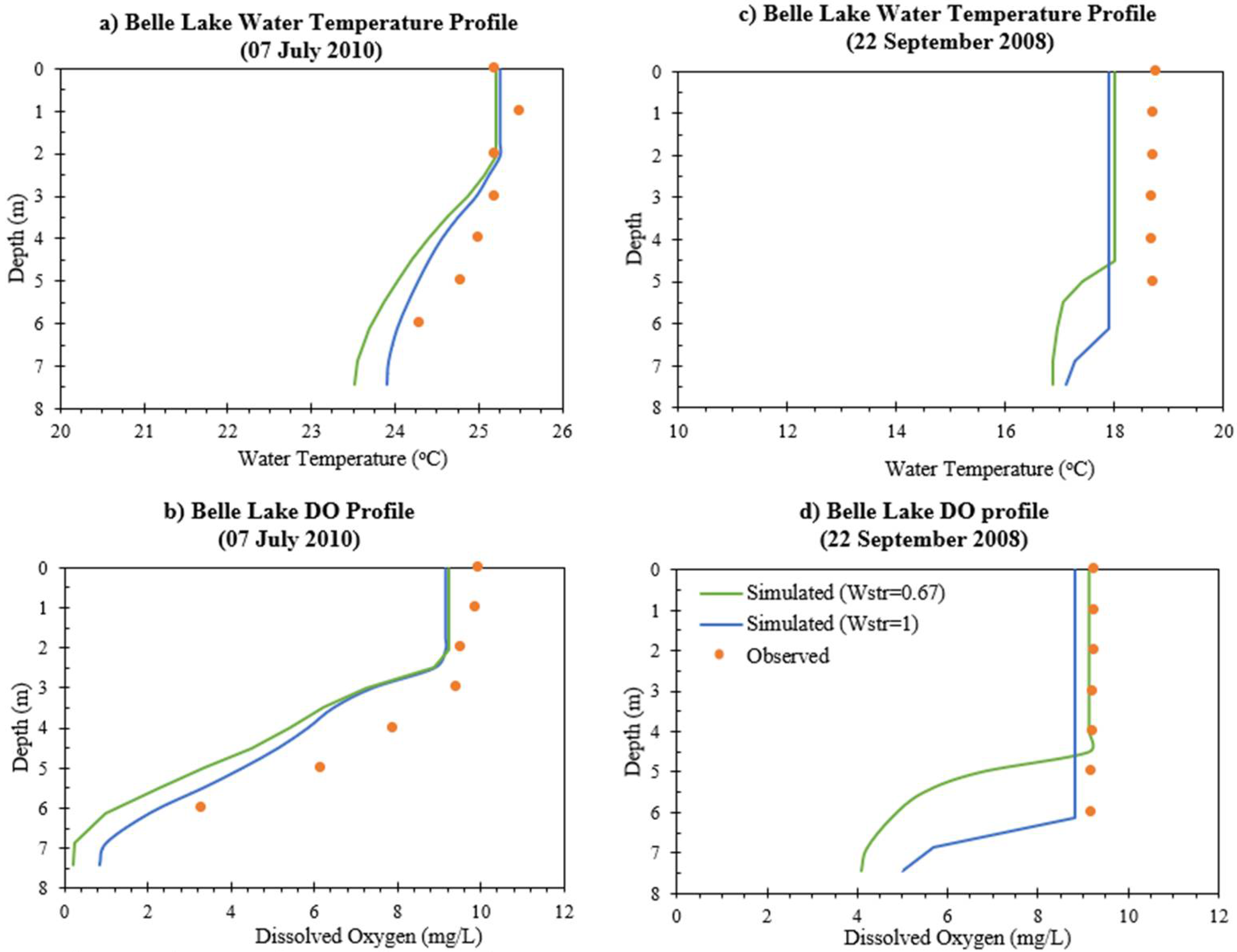
Figure 1 shows an example how the calibration affects the water temperature and DO profiles in Belle Lake. Wind sheltering coefficient is an important calibration parameter since wind is very important for mixing in a lake. However, the wind is usually obstructed by tree canopy surrounding a lake. The wind sheltering coefficient in MINLAKE model accounts for the effective portion of wind which takes part in mixing (ranges from 0 to 1). Wind sheltering coefficient of 1 ensures the wind is fully used to mix a lake water without any obstruction; therefore, it should be called the wind utilization coefficient in the future. Figure 1 shows that, on 7 July 2010 in Belle Lake, as we increased the wind sheltering coefficient, there was increased mixing and the water temperature at the hypolimnion matches better with the observed data (compared with wind sheltering coefficient of 0.67). However, on 22 September 2008, the wind sheltering coefficient affects the mixed layer depth. As the wind sheltering coefficient changed from 0.67 to 1, the mixed layer depth increased from 4.5 m to 6.2, complying with the observed data.
The results summarized in Table 4 show that for these shallow lakes, the hourly MINLAKE2018 model performed better than the daily model, especially for DO simulations, when simulated profiles were compared with observed profiles. The main reason for this improvement is the consideration of diurnal changes as illustrated by comparison of the observed and simulated temperature or DO at observed time. Table 4 shows the model performance improved significantly with the hourly model in Portage and Carrie lakes. The average root-mean-square error (RMSE) of temperature simulations in five lakes from hourly MINLAKE2018 decreased by 17.3%, and average Nash-Sutcliffe model efficiency (NSE) [36] increased by 10.3% with respect to daily model MINLAKE2012. Similarly, for the DO hourly model, average RMSE decreased by 18.2% and NSE increased by 66.7%.
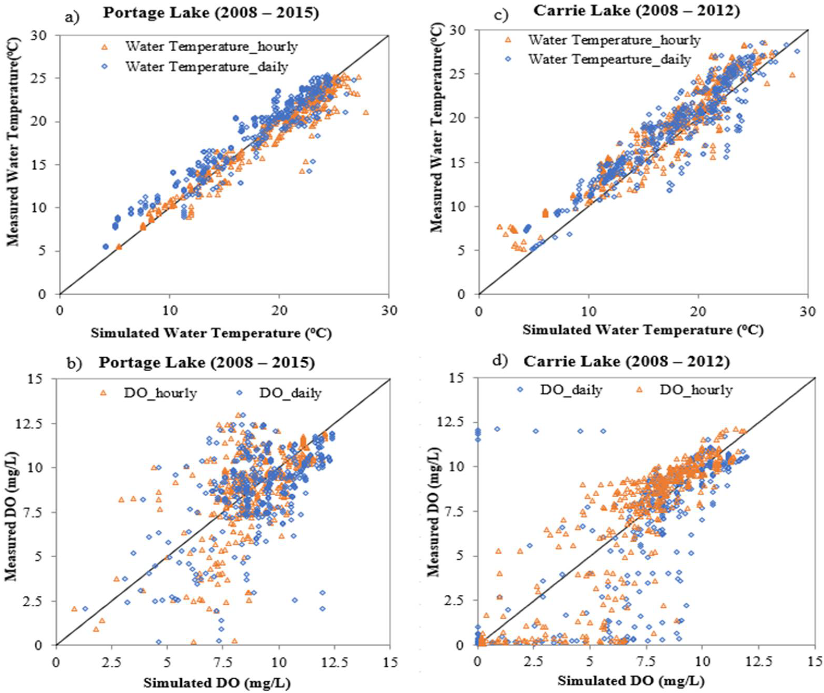
Figure 2 shows the observed water temperature and DO profile data versus simulated results using hourly and daily models in two lakes. In Figure 2a, the observed water temperatures versus daily simulated have a slope of 1.03 which means the daily model slightly underpredicts the observed water temperatures in Portage Lake. The hourly model slightly overpredicts the observed water temperatures having a slope of 0.98. In Figure 2b, the daily DO model has a slope of 0.96 whereas the hourly model has a slope of 0.99 (near 1) and performs better. Both the models slightly overpredict the observed DO. In Figure 2c, Carrie Lake daily water temperature has a slope of 1.08 whereas the hourly water temperature has a slope of 1.04. Carrie Lake daily DO has a slope of 0.92 whereas the hourly DO has a slope of 0.96. Figure 2 shows that the simulated hourly water temperature and DO match better with observed data compared to the daily model, although DO model performance still has room for improvement.
3.2. Diurnal Variations
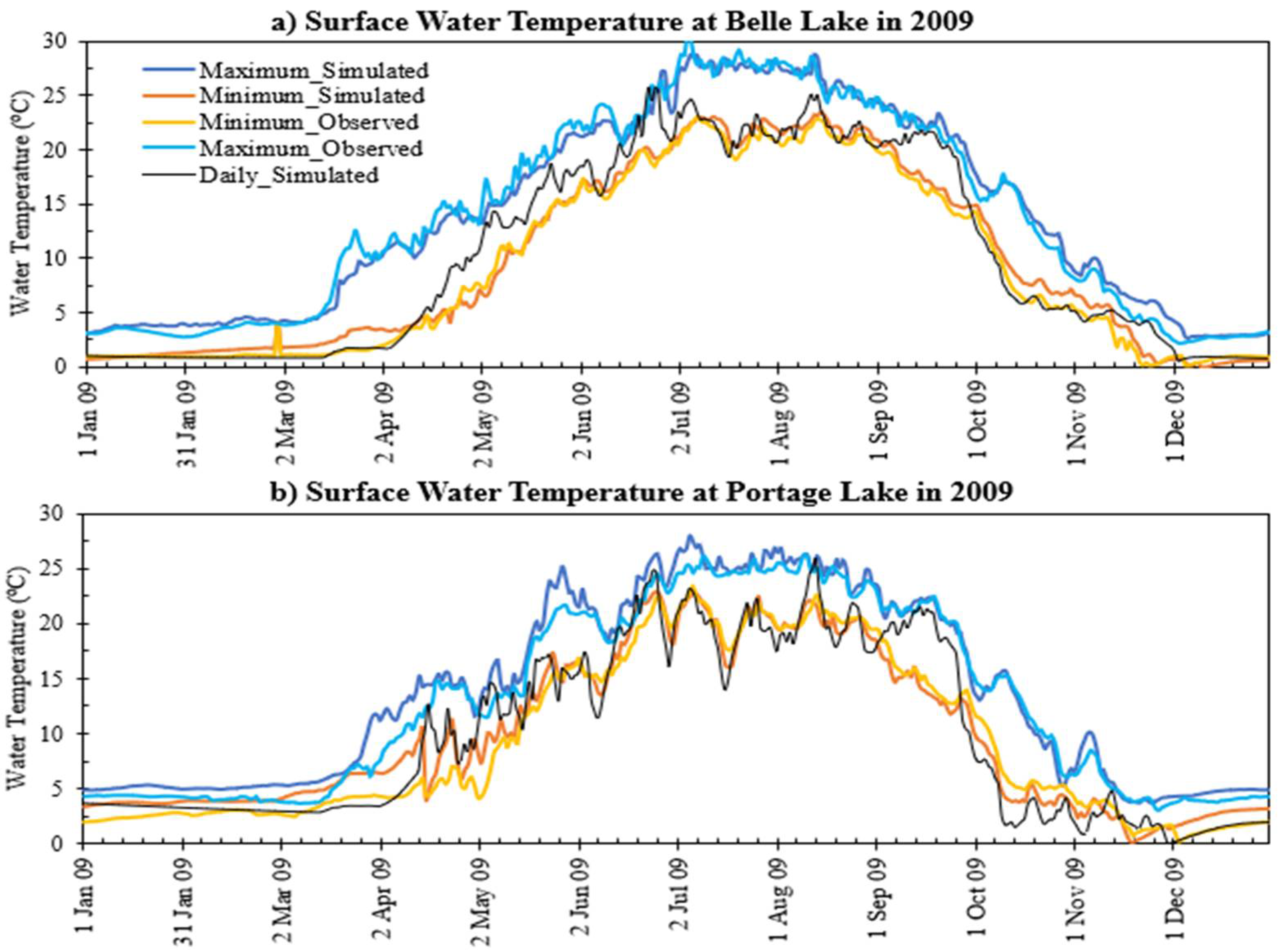
In this study, the daily MINLAKE2012 model has been successfully revised into an hourly MINLAKE2018 model by making various program changes discussed in Section 2.4. In the daily MINLAKE2012 model, the output is a single profile for the whole day. Simulated water temperatures and DO concentrations from the daily model are typically close to those of later afternoon hours. For the hourly model, 24 profiles of water temperature and DO were simulated for a day giving more detail into diurnal changes and lake processes. Figure 3 shows the simulated and observed maximum and minimum hourly surface water temperature of Portage Lake and Belle Lake during each day in 2009. The Minnesota Department of Natural Resources (MNDNR) had a long-term monitoring program to continuously measure surface water temperatures (~1 m) in a 30-min interval for 25 sentinel lakes including the five study lakes (Table 1), and a few lakes (such as Pearl Lake) had measured time-series at several depths also. Therefore, the maximum and minimum observed hourly temperatures in each day were extracted from the 30-min monitored database (MNDNR, 2018) to compare with simulated hourly results. The simulated maximum and minimum water temperatures (Figure 3) have a root mean square error (RMSE) against observed ones of 1.04 °C and 0.90 °C for Belle and 1.32 °C and 1.44 °C for Portage in 2009, respectively. At Portage Lake, the daily simulated surface temperature is close to the minimum observed surface temperature except for September. At Belle Lake, the daily simulated temperature matches well with the observed minimum hourly temperature until April, then the daily temperature lies between the maximum and minimum hourly temperature; matches with the minimum (observed or simulated) again from July to August and October to December. During September, the daily simulated temperature matches well with the maximum hourly temperature. During the winter, observed minimum and maximum temperatures are lower than simulated ones (Figure 3) because there is a strong temperature increase gradient below the ice-water interface and the water depth of the temperature sensor should reduce the ice thickness (vary with time) from the open-water depth. The diurnal temperature variations can be quantified by differences of the maximum and minimum hourly temperatures in each day and are 0.05–9.47 °C for the simulated results (mean difference 4.03 °C with a standard deviation of 2.48 °C) and 0.05–11.41 °C for the observed data (mean difference 3.69 °C with a standard deviation of 2.14 °C) at Portage Lake in 2009. The maximum water temperature occurs at 5 p.m. for 92% of the days in the open water season and at 2 p.m. for 85% of the days in the ice cover period. The minimum water temperature mostly occurs at 5 a.m. all year round (100% of days in open water season and 95% of days in the ice cover period). The average absolute difference of simulated and observed diurnal temperature variations is 0.96 °C at Portage Lake and 0.97 °C at Belle Lake in 2009. The average diurnal DO variations in each day are 0.60 mg/L (standard deviation of 0.71 mg/L and the maximum variation of 2.41 mg/L) for Belle Lake and 0.49 mg/L (standard deviation of 0.50 mg/L and the maximum variation of 5.63 mg/L) for Portage Lake for simulation results. In 2009, at Portage Lake, the maximum DO occur at 5 p.m. (because of continuous photosynthetic oxygen production in the daytime) for 95% of the days in open water season and 88% of the days in the ice cover period. The minimum DO mostly occurs at 7 a.m. all year round (95% of days in the open water season and 89% of days in the ice cover period) because of no photosynthesis during the night. There are no continuous hourly DO measurements available in the five lakes to compare with hourly simulated DO time series.
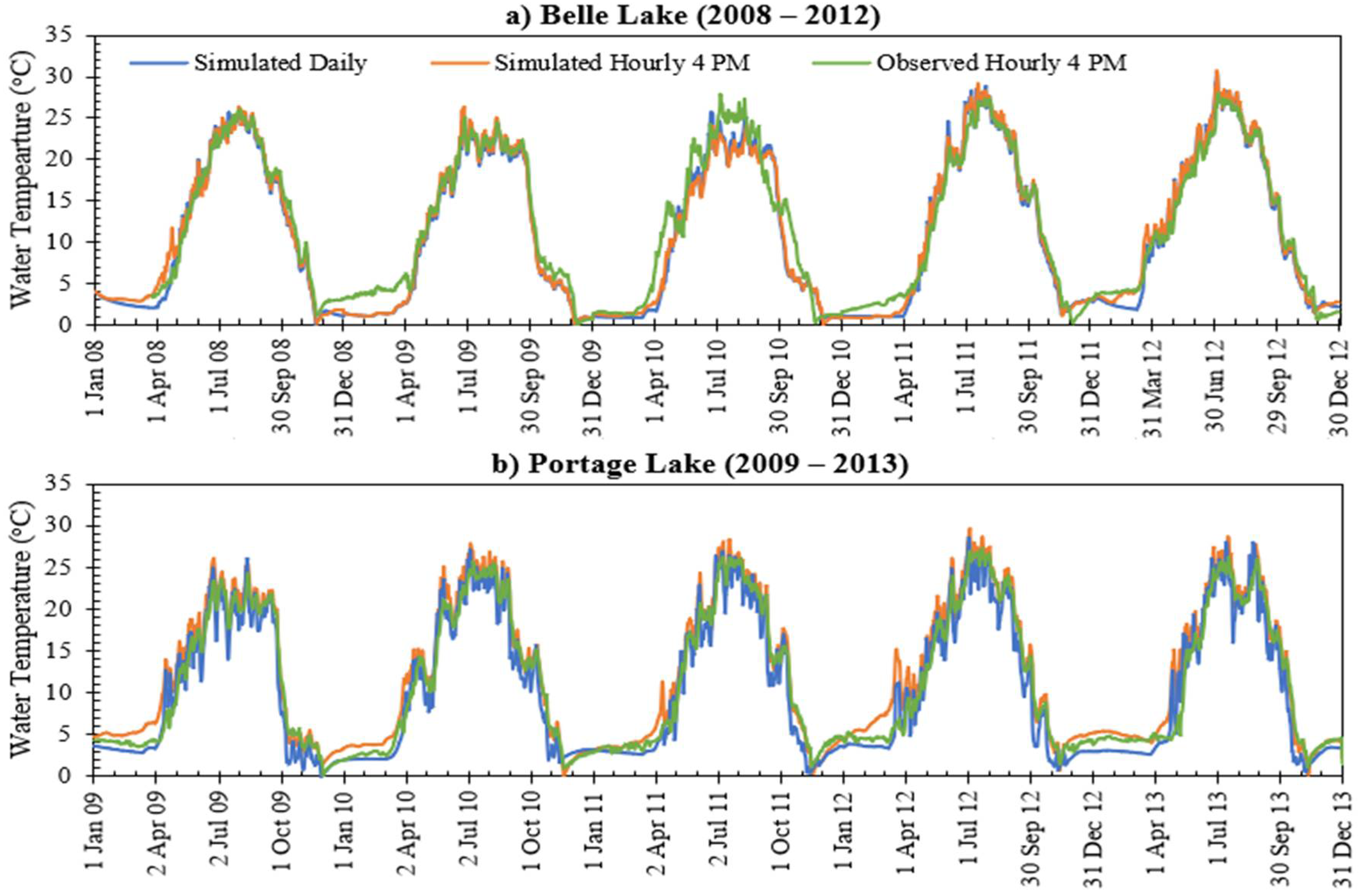
In Figure 4 the simulated daily temperatures from the daily MINLAKE2012 matched well with the observed and simulated temperatures at 4 p.m. for Belle Lake and Portage Lake over multiple years. In summer months, the simulated daily temperatures were slightly higher than observed ones but in other months slightly lower than observed. The mean difference of daily simulated water temperatures and observed water temperatures at 4 PM is 1.03 °C (standard deviation of 1.44 °C) in Belle Lake and 1.86 °C (standard deviation of 1.05 °C) in Portage Lake.
The simulated hourly temperatures at 4 PM closely follow with the observed hourly temperatures at 4 PM for 4 years in Belle and Portage Lake. The simulated and observed water temperatures at 4 PM have a mean absolute difference of 1.35 °C (standard deviation of 1.29 °C) in Belle Lake and 1.21 °C (standard deviation of 1.23 °C) in Portage Lake. For Belle Lake, simulated temperatures in 2009 winter and 2010 summer had relatively large differences from observed data; for Portage Lake, simulated temperatures slightly over-predicted in 2009–2013.
3.3. Profile Comparison
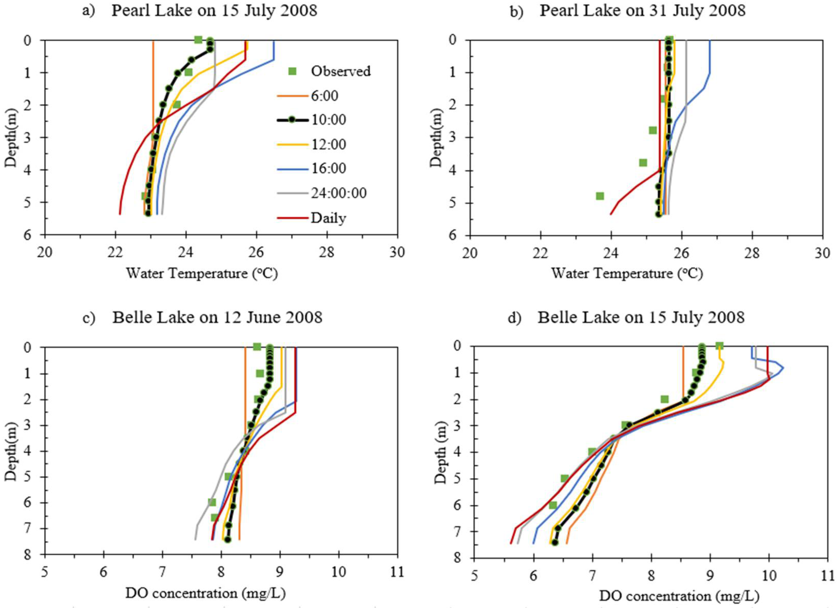
Figure 5 shows example of simulated water temperature and DO profiles for five different times throughout the day (6–24 h). Figure 5 also includes daily profiles simulated from daily MINLAKE2012 and the observed profiles in two days (water temperature) in Pearl Lake and two days (DO) in Belle Lake. The observed profiles on both days (5 June and 15 July 2008) were collected at 10:00 a.m. Therefore, the simulated profiles at 10:00 a.m. closely match the observed data. The hourly model outputs show relatively large diurnal variations in epilimnion and metalimnion, and simulated variations of DO in hypolimnion are larger than corresponding variations of temperature because there are additional DO sink terms (Equation (11)). The simulated daily profiles are reasonably close to simulated profiles at 4:00 p.m. (16:00), which is in agreement with the surface water temperature comparison shown in Figure 4. The daily model seems to overpredict stratification (surface and bottom temperature or DO difference) in those days and both lakes. On 15 July 2008, the hourly model predicts the surface DO correctly whereas overpredicts the DO in the hypolimnion at Belle Lake. For the daily model, the measured profile was compared with the simulated daily profile of water temperature or dissolved oxygen, regardless of the hour of measurement. However, for the hourly model, each observed profile can be compared with the simulated hourly profile in the observed hour and day. Simulated surface temperatures on 15 and 31 July 2008 have a diurnal variation of 3.41 and 1.63 °C in Pearl Lake, and simulated surface DO on 12 June and 15 July 2008, have a diurnal variation of 0.85 and 1.69 mg/L in Belle Lake, respectively.
3.4. Comparison of Long-Term Surface Temperature Simulation
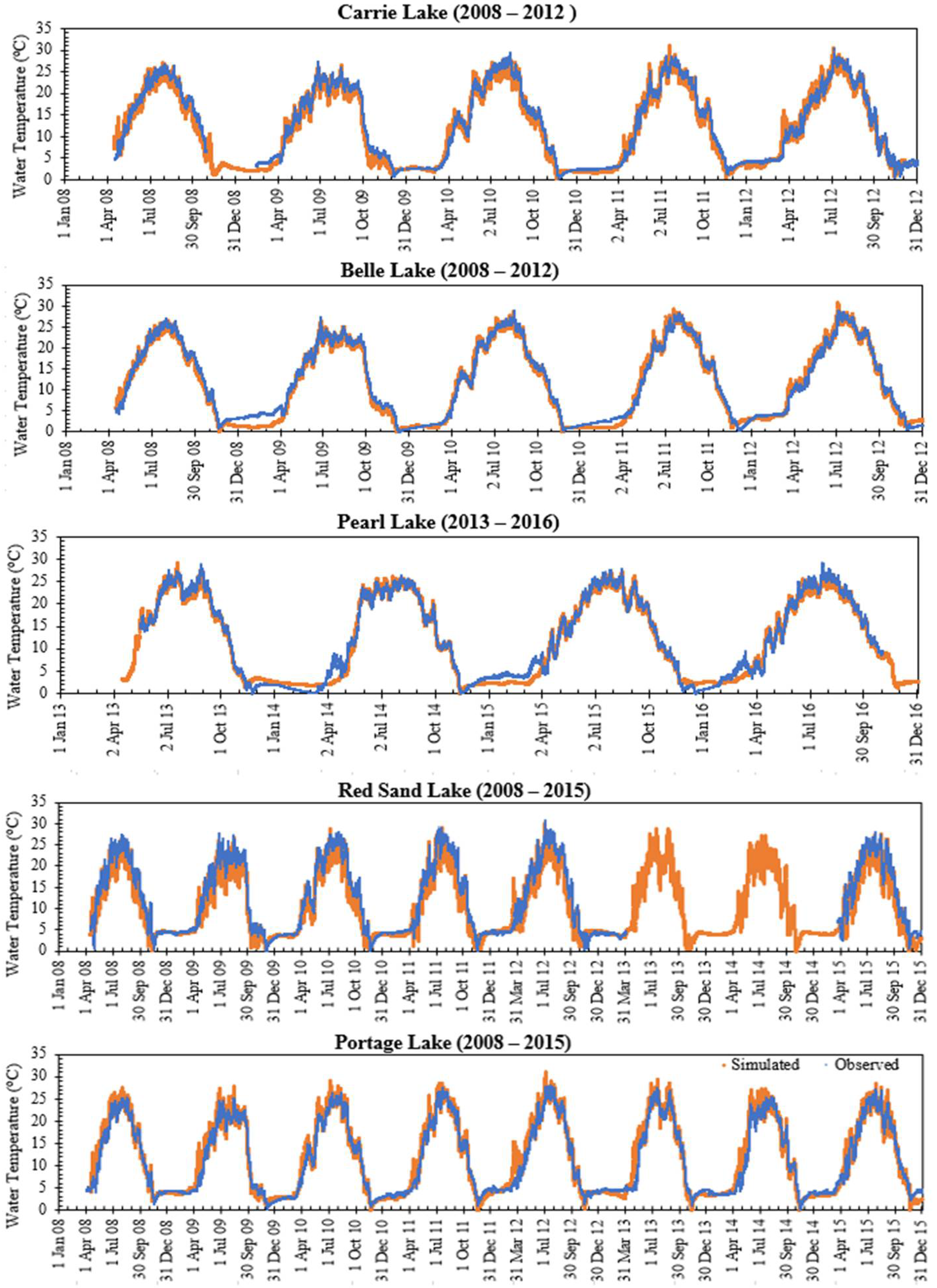
Table 5 lists the statistical parameters (RMSE, NSE, and slope) of the simulated hourly water temperatures against observed data in the five study lakes. The average RMSE of long-term water temperature simulation in the five lakes was 1.50 °C with a standard deviation of 0.32 °C. The Nash-Sutcliffe model efficiency or NSE ranges from 0.95 to 0.99, which is close to the optimal value of 1.0, and indicates the developed hourly model performs very well in comparison to observed hourly data. The slopes of 0.97–0.99 also show a good match between simulated and observed water temperature. Since Pearl Lake has observed water temperature at six depths, the error parameters were calculated at surface depth (1.2 m) and other five depths (1.7 m, 2.4 m, 3.4 m, 4.4 m, and 5 m). For Pearl Lake, the average RMSE for water temperature simulation at six different depths is 1.30 °C with a standard deviation of 0.15 °C. Figure 6 graphically shows the good performance of the hourly MINLAKE2018 against the available hourly measured data.
3.5. Comparison of Heat Flux, DO Production and Reaeration
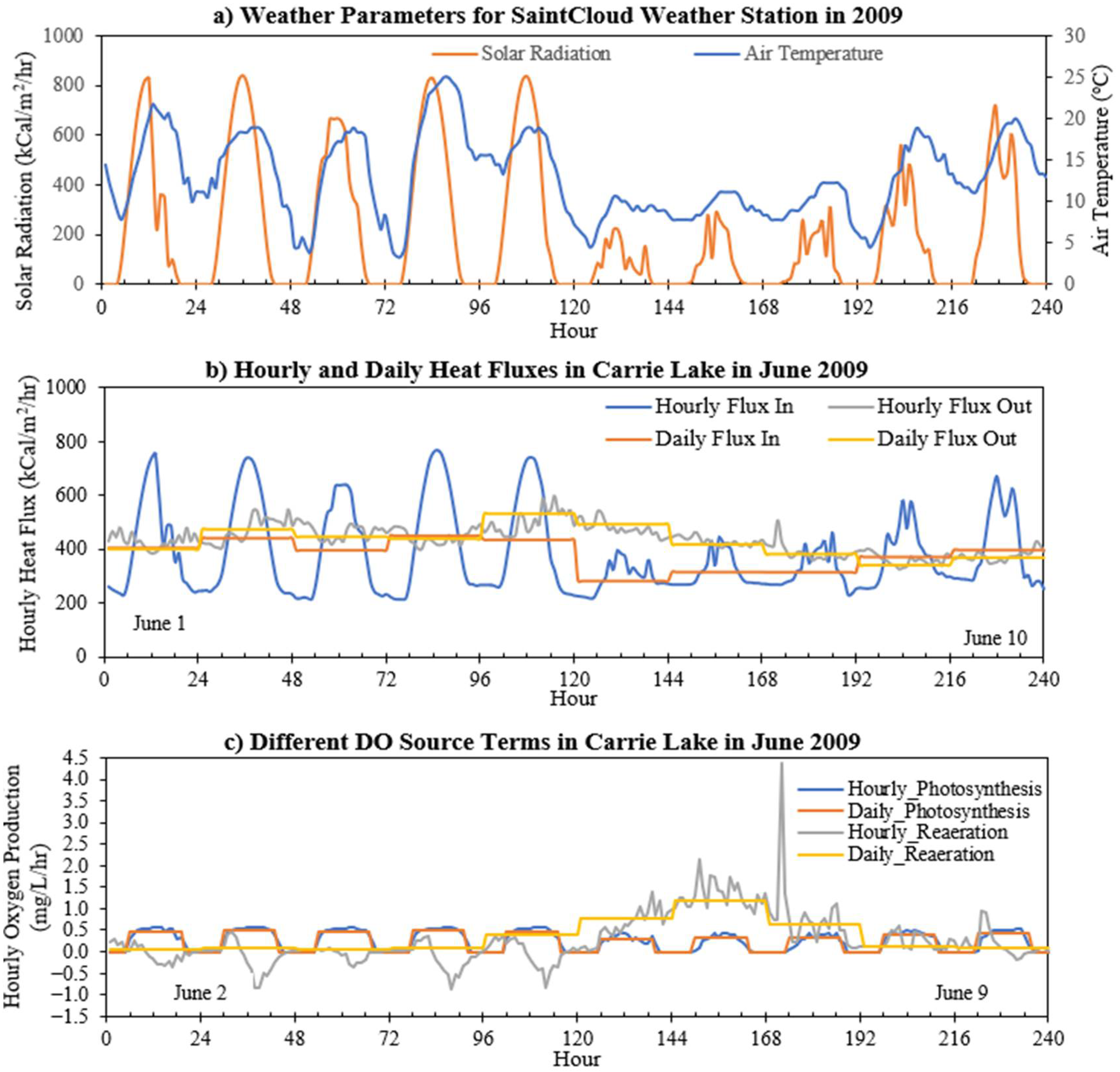
Figure 7a plots hourly air temperature and solar radiation variations and Figure 7b shows the time series of calculated hourly and daily heat fluxes that enter and exit the water surface of Carrie Lake in ten days (1 June to 10 June 2009). The daily heat flux was averaged and plotted over 24 h (Figure 7). The hourly flux in (sum of Hsn and Ha in Equation (3)) has a clear diurnal variation for most of the days while the hourly flux out (sum of Hbr, Hc, and He in Equation (3)) has almost no diurnal variation but some fluctuations in each day. At night when the solar radiation Hsn is absent, water loses heat to the atmosphere as the flux out is greater than the flux in, while during the day, due to the increase of shortwave solar radiation, the water body gains heat to increase the water temperature in epilimnion (Pearl Lake in Figure 5). The daily model has a constant heat flux in and flux out over a 24-h period whereas the hourly model considers the heat flux variations hour by hour (24 values for each day). As a result, the hourly model can represent daily variations more accurately than the daily model, which is evident in Figure 7b. Results from the daily model illustrate that heat could transfer in one direction (cooling or warming) for several consecutive days while the results from the hourly model show that heat transfer from and to the waterbody is a more dynamic process that occurs within the day and depends on the time of day.
Figure 7c shows a comparison of the time series of dissolved oxygen source terms (photosynthesis and surface reaeration) calculated by the hourly and daily models (expressed as mg/L/h). Hourly reaeration during most of the day is a sink term for the first four days of June when saturated DO (Cs in Equation (15)) is less than the surface DO concentration. On 5 June, the hourly reaeration rate is still negative whereas the daily reaeration rate is positive. From 6 June to 10 June, hourly reaeration becomes positive which means that saturated DO is higher than surface DO. On 8 June after midnight, the hourly reaeration rate suddenly increases and becomes 4.32 mg/L/h at 4 a.m. because of a strong wind speed of 19 mph (the average wind speed was 6.18 mph for the first 10 days of June at Saint Cloud). The daily model cannot account for hourly variations and has a constant reaeration rate of 0.57 mg/L/h. In the daily model, hourly photosynthesis was calculated by redistributing daily solar irradiance as a sine function over the photoperiod (14 h in June) and added together to get a daily oxygen production by photosynthesis for solving the daily DO balance equation [10], while the hourly model uses hourly solar radiation from the weather data file to get the hourly photosynthetic oxygen production and solve the hourly DO balance equation. In Figure 7c daily photosynthesis was averaged over the photoperiod starting from 6:00 a.m. to compare with hourly photosynthesis. In the presence of light, hourly photosynthetic oxygen production increases and then becomes zero during the night when there is no oxygen production. Figure 7c shows that both the hourly and daily models have similar estimates on photosynthetic oxygen production but differ in surface aeration.
3.6. Impact of Direct Solar Radiation Heating on Sediment Bed
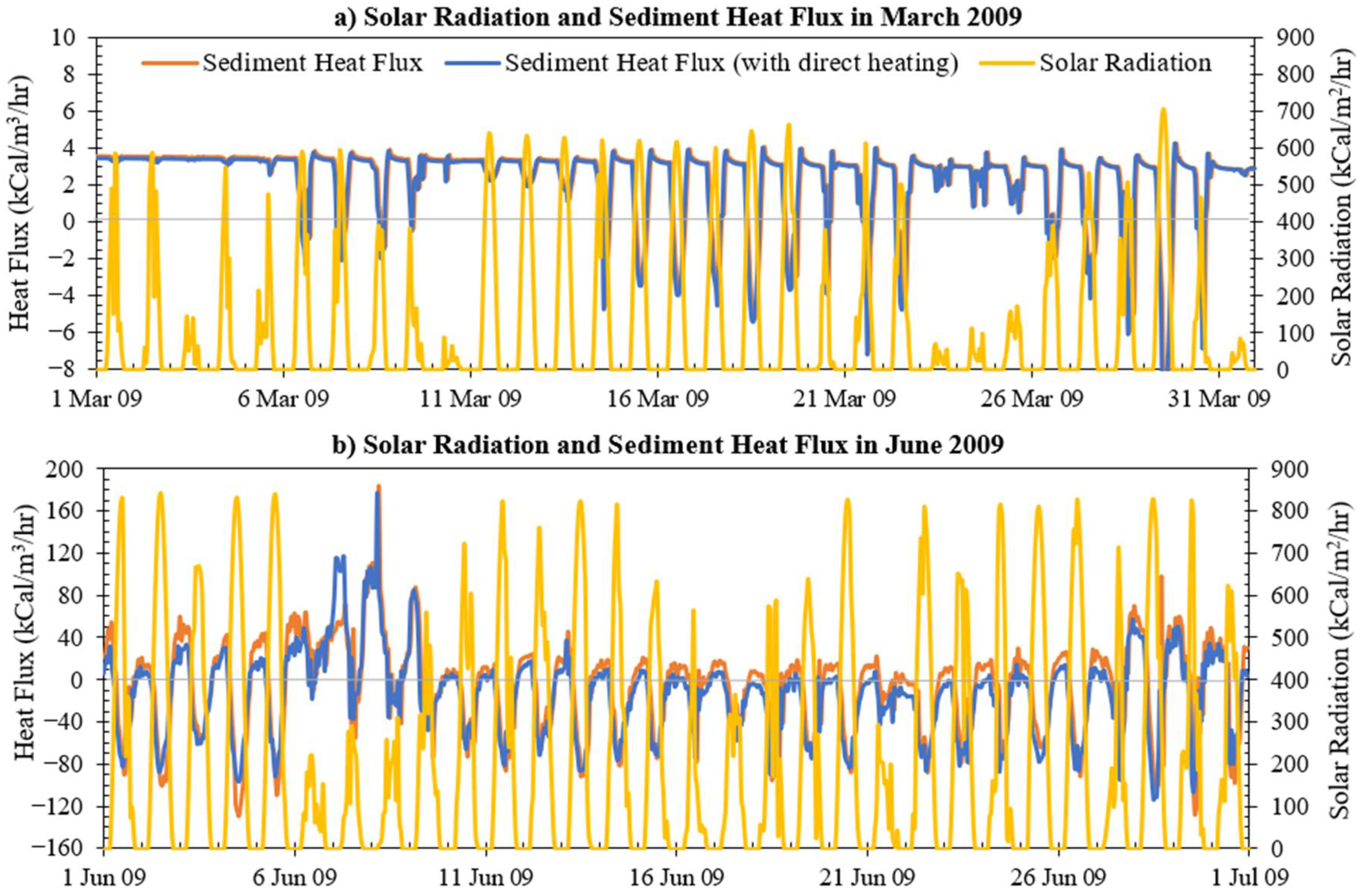
In previous MINLAKE models, the direct solar radiation heating of sediments was ignored. In the hourly MINLAKE model, the sediment heating code was modified to account for the solar radiation directly heating the sediment layers. In Figure 8 and Figure 9, a comparison was made between the previous and modified sediment heat transfer models for Carrie Lake in March and June of 2009.
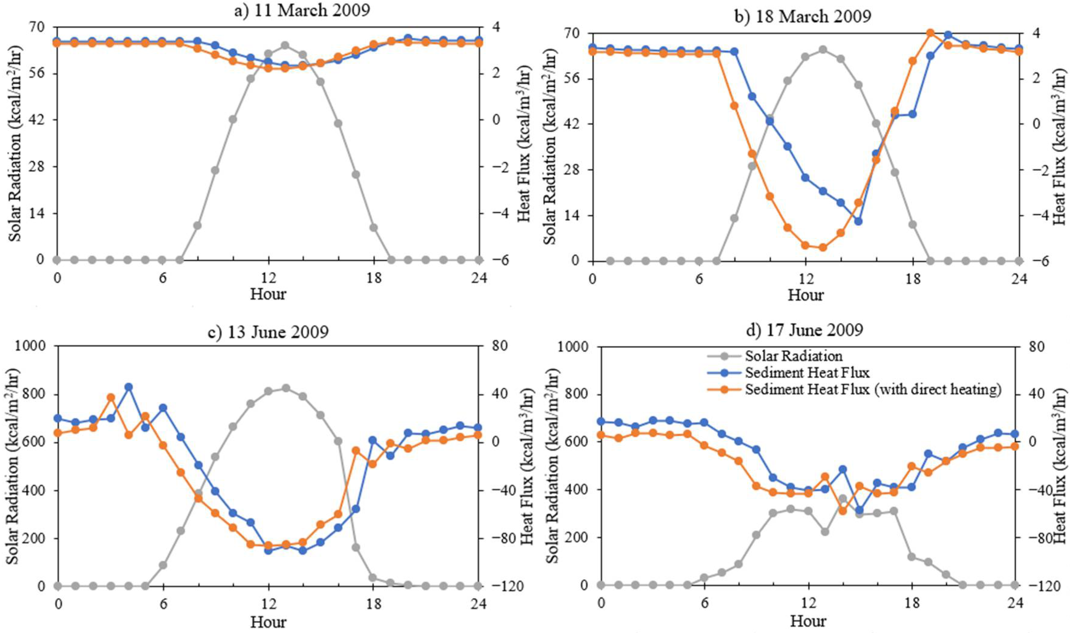
During the night when there is no solar radiation, heat moves from sediment to water, i.e., positive fluxes/numbers in Figure 8. During the day when there is incoming solar radiation, the pattern of the sediment heat flux (with direct heating) coincides with the timing of solar radiation as we are considering direct heating of sediment. In the previous sediment flux calculation, there was a time lag between the incoming solar radiation and the negative heat flux. Sediment heat flux changes in direction and magnitude depending on the solar radiation which is shown in Figure 8 for four different cases. On days with ice and snow cover, when a thin layer of snow can attenuate most of the solar radiation, heat moves from sediment to water throughout the day. On 18 March 2009, the lake has ice cover but no snow cover. The sediment heat flux starts decreasing as solar radiation heats up the water. At one point, the heat goes from water to sediment and as the water cools down at night, heat flux changes its direction again. Sediment heat flux in summer is much larger than that in winter and depends on the magnitude of solar radiation (Figure 8c for a sunny day and 8d for a cloudy day). High solar radiation results in larger negative heat flux (heat going from water to sediment) as shown in Figure 8c.
Figure 9 shows that sediment heat flux is mainly dependent on solar radiation. This addition of direct solar heating is important for the overall dynamics of shallow water layers in daytime hours. Overall, due to the modification, the modified heat flux magnitude is reduced both in positive and negative heat flux situations. As the sediment is directly heated by solar radiation, the heat flux difference between sediment and water decreases, and this trend continues throughout the entire day (24 h).
4. Discussion
4.1. Short-Term Mixing Prediction
Figure 10 shows the simulated hourly and daily water temperatures near the surface and at bottom depths in June in Belle (Hmax = 7.6 m), Carrie (Hmax = 7.9 m), and Portage (Hmax = 4.6 m) lakes. In 2009 Belle Lake was completely mixed from 6 June to 9 June and on 30 June from both the hourly and daily model simulations. On 28–29 June, the daily model results show that the lake is well mixed whereas the hourly model predicts weak stratification. This occurs due to the sudden increase in daily wind speed on those days. The hourly model simulates water temperature hour by hour using hourly wind speed which increased gradually and hence, no complete mixing was simulated by the hourly model. Carrie Lake is more stratified than Belle Lake (Figure 10b), which is related to a smaller geometry ratio (Table 1). Observed half-hourly water temperature data in these lakes were collected and converted into hourly observed data for comparison. At the surface, the simulated water temperatures match well with the observed data with an RMSE of 1.2 °C, 1.7 °C, and 1.4 °C for Belle (2008–2011), Carrie (2008–2015), and Portage (2008–2015), respectively. Since Portage is a very shallow lake with a maximum depth of 4.3 m, there are small differences between the surface and bottom water temperatures. For most of the days, the daily model predicts essentially the same temperatures at the lake surface and bottom whereas the hourly model predicts the temporal variations of water temperature more correctly. Owing to the lack of necessary details associated with the daily weather data, the daily model underpredicts the water temperature in well-mixed conditions at Portage Lake.
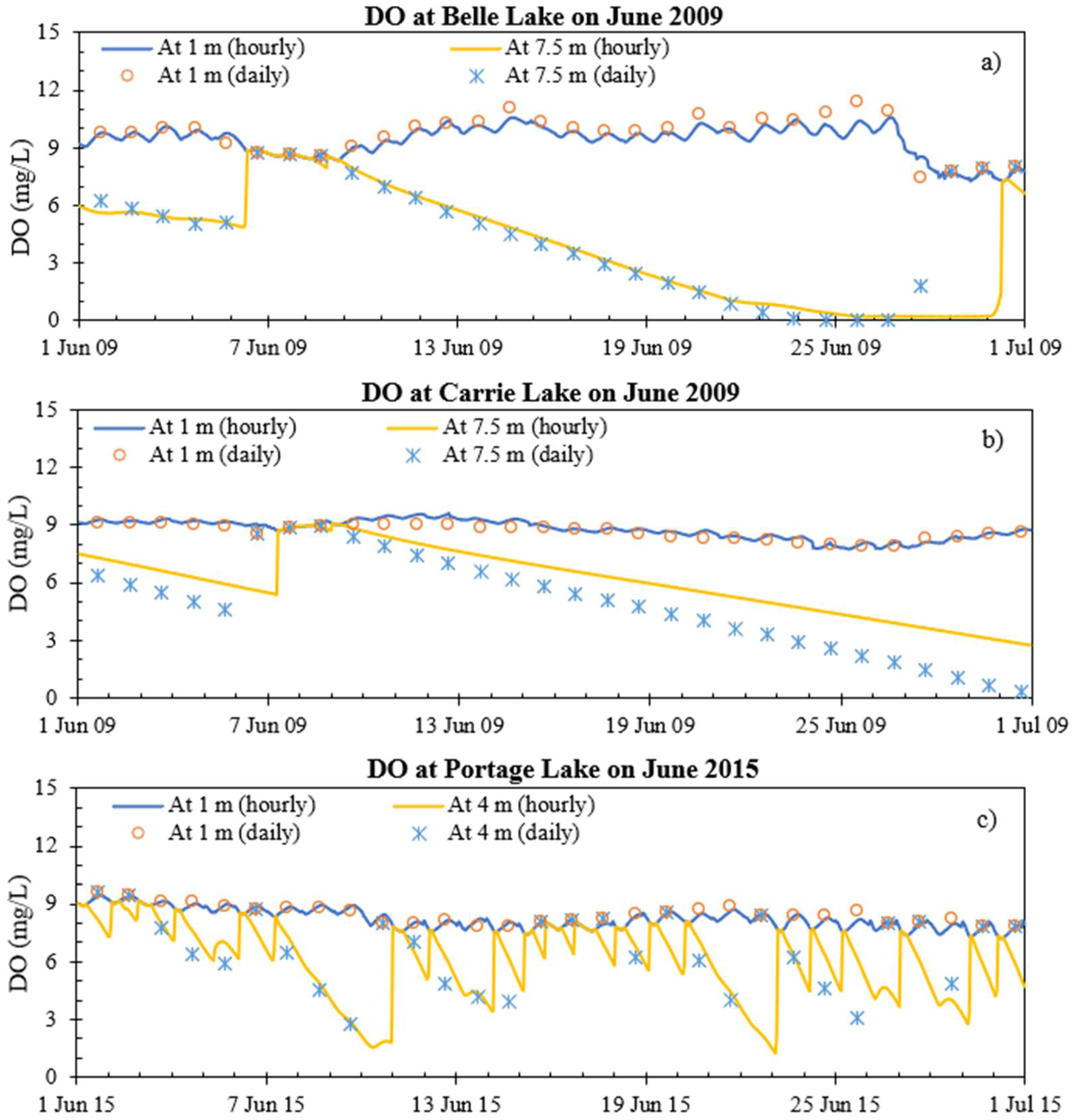
The predicted mixing from temperature simulation plays an important role in not only water temperature distribution but also dissolved oxygen (Figure 11) and nutrient concentration distributions with depth. At Belle Lake, the daily simulation represents complete mixing on 28–29 June whereas the hourly model shows anoxic condition at the lake bottom (Figure 11a). At Carrie Lake (Figure 11b), the lake becomes well mixed on 7 June whereas the hourly model simulates the low bottom DO condition on 7 June and higher DO concentrations starting from 10 June. Frequent mixing is observed in Portage Lake (Figure 11c): each day has a period of well-mixed conditions following several hours of weak stratification of DO. The daily model only accounts for the diminishing of DO from the top layer to the bottom layer and does not show the occurrence of the mixing within the day or how DO again recovers to be the same as the top layer.
4.2. Stratification Prediction
Carrie Lake has a depth of 7.9 m with a geometry ratio of 3.12. Portage Lake is comparatively shallow (4.57 m) with a geometry ratio of 7.71. From the water temperature graphs of Figure 10, it is evident that Carrie Lake is more stratified compared to Portage Lake. If the difference of water temperature or DO between the surface layer and bottom layer is more than 1 °C or 1 mg/L, the lake is considered stratified. Based on this criterion, for the hourly model, Carrie Lake is stratified 720 h (30 days) out of 720 h in June 2009 for water temperature and dissolved oxygen. However, the evaluation of stratification using the daily model reveals that the lake is stratified on 28 days in June 2009 for temperature and DO. The daily model cannot account for the mixing and stratification happening on time step shorter than a day. As a result, the daily model cannot capture the accurate scenario of stratification. For Red Sand Lake, the lake is stratified for 298 h and 359 h for water temperature and dissolved oxygen, respectively. This shows the dependence of stratification on lake depth and geometry ratio.
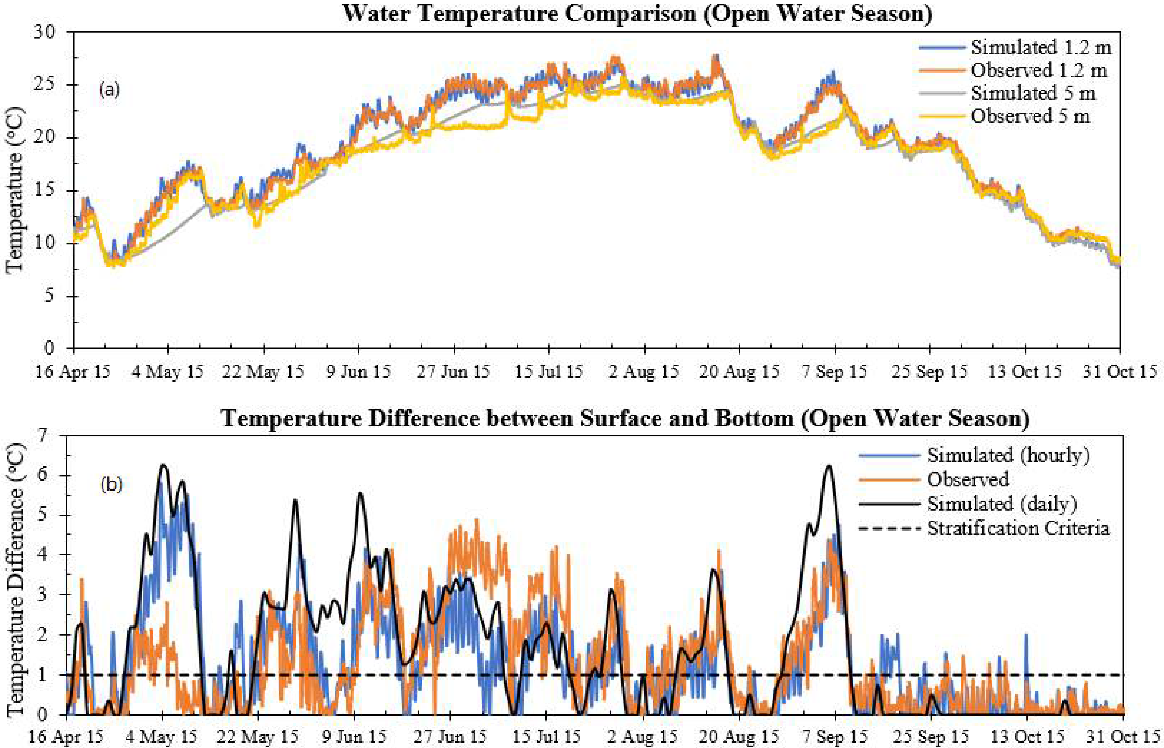
Pearl Lake has 30-min observed water temperature data that were measured from 2013 to 2016 at 6 depths (1.2, 1.7, 2.4, 3.4, 4.4, and 5.0 m) by MNDNR. The average chlorophyll-a concentration at Pearl Lake is 16.91 µg/L as a eutrophic lake and the geometry ratio is 7.71 for a weakly stratification or polymictic lake. MINLAKE2018 model was successfully run from January 2013 to December 2016, and time series of simulated temperatures in 2015 summer at 1.2 m and 5 m were compared with measured data in Figure 12.
Figure 12a shows that at 1.2 m depth near the surface, simulated hourly water temperatures match well with observed data in the open water season (1 April–30 September) of 2015. The simulated and observed hourly water temperatures at 5 m were used to verify whether the model can successfully reflect the attenuation of solar radiation and the heat diffusion mechanism inside the lake. At 5 m depth, the model underestimates the water temperature from 27 April to 9 May and overestimates from 27 June to 9 July. Apart from those periods, the model predicts water temperature at 5 m depth correctly. At 1.2 m and 5 m depths, the simulated water temperatures in 2015 have NSE values of 0.99 and 1.00, respectively, when compared with observed data.
In Figure 12b, the stratification of the lake over the same period was quantified. The stratification criterion was set as 1 °C and the observed stratification was compared with the stratification calculated by hourly and daily models. From 27 April to 9 May, the lake is stratified and the difference between the surface and bottom temperature is much larger than observed as shown in Figure 12a. From 27 May to 12 June, the hourly model represented the fluctuation of stratification correctly during this period, whereas the daily model shows continuous stratification over the entire time period. From 27 June to 9 July, for both hourly and daily models, the differences between the surface and bottom water temperature are much smaller than the observed ones as shown in Figure 12a. From 2 August to 7 August, the daily model overestimates the temperature gradient whereas the hourly model captures the temperature gradient perfectly. For the rest of the year 2015, the daily model underestimates the temperature gradient and shows no stratification during this fall season. But in reality and in the hourly model simulation, occasional stratification was observed in fall seasons. From comparing with hourly model results and observations, it reveals that the daily model cannot capture the rapid change of stratification and mixing in shallow lakes, which is one major drawback of the daily model. The daily model fails to predict stratification or mixing fluctuation, which happens for a short period, i.e., 3–6 h on some days. The daily model assumes longer periods of stratification although the shallow lakes may mix several times (each time for a few hours). Moreover, the daily model cannot correctly predict weak stratification over several hours on some days in the fall season.
The stratification statistics for five study lakes during the ice cover periods and open water seasons are given in Table 6 as percentage hours or percentage days for three years. Comparing hourly and daily models (Table 6), the major discrepancy (3–24%, average 12%) in stratification estimates happens in dissolved oxygen stratification during the ice cover period. However, in the ice cover period, for temperature stratification, there is no major discrepancy (average 5%) in the stratification scenarios of the hourly model and daily model since temperature varies only from 0 to slightly larger than 4 °C. In the open water season, some discrepancy (13–16%) for lakes with higher geometric ratios is observed. Overall, the stratification hours of dissolved oxygen increase with the change in model time step from daily to hourly.
4.3. Application in Lake Management
DO is considered to be the most important water quality parameter of a lake. With the increasing anthropogenic nutrient loading, stratification becomes increasingly important in the consumption of DO and the formation of hypoxia [37,38,39]. Hypoxia in the waterbody influence biogeochemical cycles of nutrients and exert severe negative impacts on aquatic ecosystems, such as mortality of benthic fauna, fish kills, habitat loss, and physiological stress [40,41,42]. Given the significance and the recent increase in hypoxic events in lakes, it has become necessary to enhance our understanding of the natural and anthropogenic drivers of hypoxia and the internal feedback mechanisms. Large diurnal fluctuations of oxygen between nighttime hypoxia and daytime supersaturation have been observed in shallow tidal creeks, lagoons, and estuaries [43]. It was observed that high primary production during daytime results in supersaturated DO levels, while at night respiration overwhelms the DO supply, often leading to hypoxia [44]. Variations in the extent and duration of low oxygen events can lead to substantial ecological and economic impacts. Moreover, sometimes the mixing of the inflow is very dynamic and an hourly model might be appropriate to address the change.
In Figure 5, it was observed that in the hypolimnion, the simulated daily variation of DO is larger than that of temperature because of more sink terms. This hypolimnetic DO is particularly important because it regulates the phosphorus release from sediments. High phosphorus release from lake sediments is frequently reported as an important mechanism delaying lake recovery after external loading of phosphorus has been reduced [45,46,47]. A long-term survey of 35 lakes in Europe and North America concluded that internal release of phosphorus typically continues for 10–15 years after the external loading reduction [48] but in some lakes, the internal release may last longer than 20 years [46]. In shallow lakes, it is common to observe negligible changes in phosphorus concentrations in lake water even after external load diversion [49]. For example, Lake Trummen in Sweden remained hypereutrophic even after 11 years of sewage (primary source of external loading) diversion. Finally, the removal of 1 m of high phosphorus sediment reduced the internal loading dramatically [49]. Because of the numerous physical and biogeochemical processes involved, the development of a lake water quality model that enables estimating DO responses to the external/internal environment for short intervals is essential for understanding the dynamics of hypoxia. An hourly model will be useful in scientific research of hypoxia conditions and for planning and forecasting site-specific responses to different management scenarios. They are needed to provide advice to policy-makers about the probable effectiveness of various remedial actions at affordable costs.
4.4. Future Studies
In this study, the simulated hourly water temperatures were compared with the hourly observed water temperatures near the surface for five lakes, but the hourly DO data were not available. Moreover, due to scarcity of observed profile data, all data were used for model calibration purpose. In the future, the hourly DO data should be collected and compared with hourly simulated DO to advance the hourly DO model and understand the complex DO diurnal dynamics. With long-term profile data available, the observed data should be divided into two parts: one part to be used for model calibration and the other for model validation purpose. One drawback of these model simulations was to not consider inflow to the lake which can be important for some shallow eutrophic lakes. The daily inflow/outflow model needs to be modified/improved for hourly simulation. Only five shallow lakes in Minnesota were simulated in this study. In the future, the model can be applied to more lakes of different characteristics and different climate/geographic areas and should be improved for more general use.
5. Conclusions
Both water temperature and DO in lakes exhibit noticeable diurnal changes due to changing weather conditions, and solar-radiation-dependent phytoplankton and benthic activities. The one-dimensional hourly lake water quality model MINLAKE2018 was developed from the daily MINLAKE2012 model to evaluate diurnal variations in Minnesota lakes. The simulated hourly water temperatures and DO concentrations were compared with available observed hourly near-surface water temperatures and measured temperature and DO profiles at specific times in 36–87 days (Table 4) over several years. Simulation results from the hourly MINLAKE2018 model provide the following conclusions:
- MINLAKE2018 was calibrated against measured profiles in five shallow Minnesota lakes (Table 4) with an average standard error of 1.48 °C for temperature and 2.02 mg/L for DO. With the help of available surface water temperature hourly data, the average RMSE of long-term water temperature simulation was 1.50 °C with a standard deviation of 0.32 °C. For Pearl Lake, the average RMSE for water temperature simulation at six different depths is 1.30 °C with a standard deviation of 0.15 °C.
- When compared with the daily MINLAKE2012 model, for Pearl Lake (Hmax = 5.6 m), the hourly model calculated 12% and 13% more temperature stratification for ice cover period and open water season, respectively (Table 6). Similarly, for DO, stratification increases were 14% and 20% for ice cover period and open water season, respectively. For other lakes, hourly model simulation also resulted in increased stratification percentages for water temperature and DO. The hourly model can capture diurnal changes and mixing events that lasted a few hours within a day, which the daily model ignores. Moreover, it was observed that the daily model could not predict most of the weak stratifications of shallow lakes in the fall season (Figure 12). As a result, to ensure desired water quality for aquatic organisms and fish habitat, the hourly model is suitable for shallow lakes all year round.
- The hourly model MINLAKE2018 performs better than the daily model MINLAKE2012 in water temperature and DO profile simulation (Figure 2). The RMSEs of temperature and DO from MINLAKE2018 decreased by 17.3% and 18.2%, respectively, and Nash-Sutcliffe efficiency increased by 10.3% and 66.7%, respectively, in comparison to MINLAKE2012.
- Sediment heating subroutine was modified to include direct heating of sediment from solar radiation for all sediment layers. After modification, the sediment heat flux pattern became coincident with the solar radiation pattern eliminating the lag time between the change in solar radiation and the change in heat flux to appear. The magnitude of sediment heat flux was reduced for both cases (heat flux going from water to sediment or sediment to water) after the sediment subroutine was modified.
Author Contributions
B.T. developed the final version of the MINLAKE2018 program, conducted the simulations, analyzed the result, and prepared the manuscript draft and revisions. J.A.J. developed the first version of the program and prepared input data for lakes. X.F. supervised model development, simulation runs, data analysis, and revised the manuscript. Y.Z. and J.S.H. supervised the writing and revised the manuscript. All authors made contributions to the study and writing the manuscript. All authors have read and agreed to the published version of the manuscript.
Funding
The study is partially supported by funding from the OUC-AU Joint Center for Aquaculture and Environmental Science for the project “Forecasting the Ecological Health of Coastal Waters in Alabama and China.” Alan E. Wilson is PI, Xing Fang and Joel Hayworth are Co-PIs at Auburn University; Sun Dajiang is PI, Yangen Zhou, Kai You, and Hongwei Shan are Co-PIs from OUC (Ocean University of China).
Institutional Review Board Statement
Not applicable.
Informed Consent Statement
Not applicable.
Data Availability Statement
Some or all data, models, or code generated or used during the study are proprietary or confidential and may only be provided with restrictions. The model input and output data are specifically designed for a research numerical model. They are available upon request but are not useful for the general public.
Conflicts of Interest
The authors declare no conflict of interest.
References
- Coutant, C.C. Striped bass, temperature, and dissolved oxygen: A speculative hypothesis for environmental risk. Trans. Am. Fish. Soc. 1985, 14, 31–61. [Google Scholar] [CrossRef]
- USACE. CE-QUAL-R1: A Numerical One-Dimensional Model of Reservoir Water Quality; User’s Manual; U.S. Army Corps of Engineers Waterways Experiment Station: Vicksburg, MS, USA, 1995.
- Chapra, S.C. Surface Water-Quality Modeling; Waveland Press: Salem, WI, USA, 2008. [Google Scholar]
- Fang, X.; Jiang, L.; Jacobson, P.C.; Fang, N.Z. Simulation and validation of cisco habitat in Minnesota lakes using the lethal-niche-boundary curve. Br. J. Environ. Clim. Chang. 2014, 4, 444–470. [Google Scholar] [CrossRef]
- Riley, M.J.; Stefan, H.G. MINLAKE: A dynamic lake water quality simulation model. Ecol. Model. 1988, 43, 155–182. [Google Scholar] [CrossRef]
- Fang, X.; Alam, S.R.; Stefan, H.G.; Jiang, L.; Jacobson, P.C.; Pereira, D.L. Simulations of water quality and oxythermal cisco habitat in Minnesota lakes under past and future climate scenarios. Water Qual. Res. J. Can. 2012, 47, 375–388. [Google Scholar] [CrossRef]
- Riley, M.J.; Stefan, H.G. Dynamic Lake Water Quality Simulation Model “MINLAKE"; St. Anthony Falls Hydraulic Laboratory, University of Minnesota: Minneapolis, MN, USA, 1987; 140p. [Google Scholar]
- Fang, X.; Stefan, H.G. Modeling of Dissolved Oxygen Stratification Dynamics in Minnesota Lakes under Different Climate Scenarios; St. Anthony Falls Hydraulic Laboratory, University of Minnesota: Minneapolis, MN, USA, 1994; 260p. [Google Scholar]
- Hondzo, M.; Stefan, H.G. Regional water temperature characteristics of lakes subjected to climate change. Clim. Chang. 1993, 24, 187–211. [Google Scholar] [CrossRef]
- Stefan, H.G.; Fang, X. Dissolved oxygen model for regional lake analysis. Ecol. Model. 1994, 71, 37–68. [Google Scholar] [CrossRef]
- Fang, X.; Stefan, H.G. Temperature and Dissolved Oxygen Simulations for a Lake with Ice Cover; Project Report 356; St. Anthony Falls Hydraulic Laboratory, University of Minnesota: Minneapolis, MN, USA, 1994. [Google Scholar]
- Fang, X.; Stefan, H.G. Dynamics of heat exchange between sediment and water in a lake. Water Resour. Res. 1996, 32, 1719–1727. [Google Scholar] [CrossRef]
- Fang, X.; Ellis, C.R.; Stefan, H.G. Simulation and observation of ice formation (freeze-over) in a lake. Cold Reg. Sci. Technol. 1996, 24, 129–145. [Google Scholar] [CrossRef]
- Fang, X.; Alam, S.R.; Jacobson, P.; Pereira, D.; Stefan, H.G. Simulations of Water Quality in Cisco Lakes in Minnesota; St. Anthony Falls Laboratory: Minneapolis, MN, USA, 2010. [Google Scholar]
- Xu, Z.; Xu, Y.J. A deterministic model for predicting hourly dissolved oxygen change: Development and application to a shallow eutrophic lake. Water 2016, 8, 41. [Google Scholar] [CrossRef]
- Martin, J.L. Hydro-Environmental Analysis: Freshwater Environments; CRC Press: Boca Raton, FL, USA, 2013. [Google Scholar]
- Heddam, S. Modeling hourly dissolved oxygen concentration (DO) using two different adaptive neuro-fuzzy inference systems (ANFIS): A comparative study. Environ. Monit. Assess. 2013, 186, 597–619. [Google Scholar] [CrossRef]
- Kisi, O.; Alizamir, M.; Gorgij, A.D. Dissolved oxygen prediction using a new ensemble method. Environ. Sci. Pollut. Res. 2020, 27, 9589–9603. [Google Scholar] [CrossRef] [PubMed]
- Granger, R.J.; Hedstrom, N. Modelling hourly rates of evaporation from small lakes. Hydrol. Earth Syst. Sci. 2011, 15, 267–277. [Google Scholar] [CrossRef] [Green Version]
- Hondzo, M.; Stefan, H.G. Lake water temperature simulation model. J. Hydraul. Eng. 1993, 119, 1251–1273. [Google Scholar] [CrossRef]
- Jamily, J.A. Developing an Hourly Water Quality Model to Simulate Diurnal Water Temperature and Dissovled Oxygen Variations in Shallow Lakes; Auburn University: Auburn, AL, USA, 2018. [Google Scholar]
- Gu, R.; Stefan, H.G. Year-round temperature simulation of cold climate lakes. Cold Reg. Sci. Technol. 1990, 18, 147–160. [Google Scholar] [CrossRef]
- Ji, Z.-G. Hydrodynamics and Water Quality: Modeling Rivers, Lakes, and Estuaries; John Wiley & Sons: Hoboken, NJ, USA, 2008. [Google Scholar]
- Megard, R.O.; Tonkyn, D.W.; Senft, W.H. Kinetics of oxygenic photosynthesis in planktonic algae. J. Plankton Res. 1984, 6, 325–337. [Google Scholar] [CrossRef]
- Holley, E. Oxygen transfer at the air-water interface. Transp. Process. Lakes Ocean. 1977, 7, 117. [Google Scholar]
- Thomann, R.V.; Mueller, J.A. Principles of Surface Water Quality Modeling and Control; Harper Collins Publishers Inc.: New York, NY, USA, 1987; p. xii. [Google Scholar]
- Utley, B.C.; Vellidis, G.; Lowrance, R.; Smith, M.C. Factors affecting sediment oxygen demand dynamics in blackwater streams of Georgia’s coastal plain. J. Am. Water Resour. Assoc. 2008, 44, 742–753. [Google Scholar] [CrossRef]
- Truax, D.D.; Shindala, A.; Sartain, H. Comparison of two sediment oxygen demand measurement techniques. J. Environ. Eng. 1995, 121, 619–624. [Google Scholar] [CrossRef]
- Fang, X.; Stefan, H.G. Long-term lake water temperature and ice cover simulations/measurements. Cold Reg. Sci. Technol. 1996, 24, 289–304. [Google Scholar] [CrossRef]
- Fang, X.; Stefan, H.G. Temperature variability in the lake sediments. Water Resour. Res. 1998, 34, 717–729. [Google Scholar] [CrossRef]
- Fang, X.; Stefan, H.G.; Davis, M.B. Status of Climate Change Effect Simulations for Mirror Lake, New Hampshire; St. Anthony Falls Hydraulic Laboratory, University of Minnesota: Minneapolis, MN, USA, 1993; 52p. [Google Scholar]
- Walters, R.A.; Carey, G.F.; Winter, D.F. Temperature computation for temperate lakes. Appl. Math. Mod. 1978, 2, 41–48. [Google Scholar] [CrossRef]
- Wang, B.; Ma, Y.; Ma, W.; Su, Z. Physical control on half-hourly, daily and monthly turbulent flux and energy budget over a high-altitude small lake on the Tibetan Plateau. J. Geophys. Res. Atmos. 2017, 122, 2289–2303. [Google Scholar] [CrossRef]
- NAS; NAE. Water Quality Criteria 1972—A Report of the Committee on Water Quality Criteria; Environmental Protection Agency: Washington, DC, USA, 1973.
- Fang, X.; Stefan, H.G. Chapter 16 Impacts of Climatic Changes on Water Quality and Fish Habitat in Aquatic Systems. In Handbook of Climate Change Mitigation; Chen, W.-Y., Seiner, J.M., Suzuki, T., Lackner, M., Eds.; Springer: Berlin/Heidelberg, Germany, 2012; Volume 1, pp. 531–570. [Google Scholar]
- Nash, J.E.; Sutcliffe, J.V. River flow forecasting through conceptual models part I—A discussion of principles. J. Hydrol. 1970, 10, 282–290. [Google Scholar] [CrossRef]
- Buzzelli, C.P.; Powers, S.P.; Luettich, R.A., Jr.; McNinch, J.E.; Peterson, C.H.; Pinckey, J.L.; Paerl, H.W. Estimating the spatial extent of bottom water hypoxia and benthic fishery habitat degradation in the Neuse River Estuary, NC. Mar. Ecol. Prog. Ser. 2002, 230, 103–112. [Google Scholar] [CrossRef]
- Waldhauer, R.; Draxler, A.F.J.; McMillan, D.G.; Zetlin, C.A.; Leftwich, S.; Matte, A.; O’Reilly, J.E. Biological, physical and chemical dynamics along a New York Bight transect and their relation to hypoxia. Estuaries 1985, 8, 129. [Google Scholar]
- Yin, K.; Lin, Z.; Ke, Z. Temporal and spatial distribution of dissolved oxygen in the Pearl River Estuary and adjacent coastal waters. Cont. Shelf Res. 2004, 24, 1935–1948. [Google Scholar] [CrossRef] [Green Version]
- Pena, M.A.; Katsev, S.; Oguz, T.; Gilbert, D. Modeling dissolved oxygen dynamics and hypoxia. Biogeosciences 2010, 7, 933–957. [Google Scholar] [CrossRef] [Green Version]
- Levin, L.A.; Ekau, W.; Gooday, A.J.; Jorissen, F.; Middelburg, J.; Naqvi, J.; Neira, S.W.A.; Rabalais, N.N.; Zhang, F. Effects of natural and human-induced hypoxia on coastal benthos. Biogeosciences 2009, 6, 2063–2098. [Google Scholar] [CrossRef] [Green Version]
- Ekau, W.; Auel, H.; Portner, H.O.; Gilbert, D. Impacts of hypoxia on the structure and processes in the pelagic community (zooplankton, macro-invertebrates and fish). Biogeosciences 2009, 6, 5073–5144. [Google Scholar]
- D’ Avanzo, C.; Kremer, J.N. Diel oxygen dynamics and anoxic events in an eutrophic estuary of Waquoit Bay, Massachusetts. Estuaries 1994, 171, 131–139. [Google Scholar] [CrossRef]
- Shen, J.; Wang, T.; Herman, J.; Masson, P.; Arnold, G.L. Hypoxia in a coastal embayment of the Chesapeake Bay: A model diagnostic study of oxygen dynamics. Estuaries Coasts 2008, 31, 652–663. [Google Scholar] [CrossRef]
- Marsden, M.W. Lake restoration by reducing external phosphorus loading; the influence of sediment phosphorus release. Freshw. Biol. 1989, 21, 139–162. [Google Scholar] [CrossRef]
- Sondergaard, M.; Jeppesen, E.; Jensen, J.P.; Amsinck, S.L. Water framework directive: Ecological classification of Danish lakes. J. Appl. Ecol. 2005, 42, 616–629. [Google Scholar] [CrossRef]
- Philips, G.; Kelly, A.; Pitt, J.A.; Sanderson, R.; Taylor, E. The recovery of a very shallow eutrophic lake, 20 years after the control of effluent derived phosphorus. Freshw. Biol. 2005, 50, 1628–1638. [Google Scholar] [CrossRef]
- Jeppesen, E.; Sondergaard, M.; Jensen, J.P.; Havens, K.E.; Anneville, O.; Carvalho, L.; Coveney, M.F.; Deneke, R.; Dokulil, M.T.; Foy, B.; et al. Lake responses to reduced nutrient loading: An analysis of contemporary long-term data from 35 case studies. Freshw. Biol. 2005, 50, 1747–1771. [Google Scholar] [CrossRef]
- Welch, E.B.; Cooke, G.D. Internal phosphorus loading in shallow lakes: Importance and control. Lake Reserv. Manag. 2009, 21, 209–217. [Google Scholar] [CrossRef] [Green Version]
Figure 1.
Effect of wind sheltering coefficient (increasing from 0.67 to 1) on simulated (a) water temperature and (b) dissolved oxygen profiles on 7 July 2010; (c) water temperature and (d) dissolved oxygen profiles on 22 September 2008 in Belle Lake including observed profiles.
Figure 1.
Effect of wind sheltering coefficient (increasing from 0.67 to 1) on simulated (a) water temperature and (b) dissolved oxygen profiles on 7 July 2010; (c) water temperature and (d) dissolved oxygen profiles on 22 September 2008 in Belle Lake including observed profiles.

Figure 2.
Measured versus simulated water temperature and DO in Portage Lake and Carrie Lake for simulation over several years.
Figure 2.
Measured versus simulated water temperature and DO in Portage Lake and Carrie Lake for simulation over several years.

Figure 3.
Time series of simulated and observed maximum and minimum hourly surface water temperatures each day at (a) Portage Lake and (b) Belle Lake in 2009 including simulated daily temperatures.
Figure 3.
Time series of simulated and observed maximum and minimum hourly surface water temperatures each day at (a) Portage Lake and (b) Belle Lake in 2009 including simulated daily temperatures.

Figure 4.
Time series of simulated daily, simulated and observed hourly surface (1 m at Belle and 1.5 m at Portage Lake) temperatures at 4 PM at Belle Lake (2008–2012) and Portage Lake (2009–2013).
Figure 4.
Time series of simulated daily, simulated and observed hourly surface (1 m at Belle and 1.5 m at Portage Lake) temperatures at 4 PM at Belle Lake (2008–2012) and Portage Lake (2009–2013).

Figure 5.
Simulated water temperature profiles in Pearl Lake and DO profiles in Belle Lake at five different hours comparing with observed (green squares) and simulated daily profiles.
Figure 5.
Simulated water temperature profiles in Pearl Lake and DO profiles in Belle Lake at five different hours comparing with observed (green squares) and simulated daily profiles.

Figure 6.
Time series of observed (orange) and simulated (blue) hourly surface water temperatures in five study lakes over 4–8 years of simulation.
Figure 6.
Time series of observed (orange) and simulated (blue) hourly surface water temperatures in five study lakes over 4–8 years of simulation.

Figure 7.
Time series of (a) air temperature and solar radiation, (b) calculated daily and hourly heat fluxes, and (c) two DO source terms through the water surface at Carrie Lake on 1–10 June 2009.
Figure 7.
Time series of (a) air temperature and solar radiation, (b) calculated daily and hourly heat fluxes, and (c) two DO source terms through the water surface at Carrie Lake on 1–10 June 2009.

Figure 8.
Comparison of heat flux calculated by the modified and previous sediment models on an hourly basis on (a) day with ice and snow cover, (b) day with ice cover but no snow cover, (c) high solar radiation day in June, (d) low solar radiation day in June. The y-axis scales on (a,b) are different from on (c,d).

Figure 9.
Sediment heat flux distribution in (a) March 2009 and (b) June 2009 in Carrie Lake.

Figure 10.
Time series of simulated daily and hourly water temperatures at two depths (1 m, 7.5 or 4 m) at (a) Belle Lake in June 2009, (b) Carrie Lake in June 2009, and (c) Portage Lake in June 2015 including observed hourly surface temperatures. Daily values were plotted at 4:00 p.m. each day.
Figure 10.
Time series of simulated daily and hourly water temperatures at two depths (1 m, 7.5 or 4 m) at (a) Belle Lake in June 2009, (b) Carrie Lake in June 2009, and (c) Portage Lake in June 2015 including observed hourly surface temperatures. Daily values were plotted at 4:00 p.m. each day.

Figure 11.
Time series of simulated daily and hourly DO at two depths (1 m, 7.5 or 4 m) at (a) Belle Lake in June 2009, (b) Carrie Lake in June 2009, and (c) Portage Lake in June 2015. Daily values were plotted at 4:00 p.m. each day.
Figure 11.
Time series of simulated daily and hourly DO at two depths (1 m, 7.5 or 4 m) at (a) Belle Lake in June 2009, (b) Carrie Lake in June 2009, and (c) Portage Lake in June 2015. Daily values were plotted at 4:00 p.m. each day.

Figure 12.
(a) Time series of observed and simulated hourly water temperature at 1.2 m and 5 m in Pearl Lake in open water season in 2015, (b) differences of simulated and observed hourly temperatures between 1.2 m (surface) and 5 m (near the bottom) during open water season in 2015 in Pearl Lake including simulated daily temperature differences and 1 °C difference as stratification criterion.


Table 1.
Characteristics of five study lakes in Minnesota.
| Lake | Surface Area, As, (km2) | Max. Depth Hmax, (m) | Geometry Ratio 1 (m)0.5 | Mean Chl-a (μg/L) | Trophic Status | Simulation Years | Number of Days with Profile Data |
|---|---|---|---|---|---|---|---|
| Carrie | 0.37 | 7.90 | 3.12 | 6.71 | Mesotrophic | 2008–2012 | 50 |
| Belle | 3.71 | 7.60 | 5.77 | 27.10 | Eutrophic | 2008–2012 | 73 |
| Pearl | 3.05 | 5.55 | 7.53 | 16.91 | Eutrophic | 2008–2012 | 36 |
| Portage | 1.54 | 4.57 | 7.71 | 15.98 | Eutrophic | 2008–2015 | 86 |
| Red Sand | 2.11 | 4.57 | 8.34 | 4.43 | Mesotrophic | 2008–2015 | 87 |
Note: 1 Geometry ratio of a lake is As0.25/Hmax where As in m2 and Hmax in m.
Table 2.
Calibration parameters for hourly and daily MINLAKE models [35].
Table 2.
Calibration parameters for hourly and daily MINLAKE models [35].
| Calibration Parameter | Effect on Model Results | Description of the Parameter |
|---|---|---|
| Wstr | Temperature and DO profiles | Wind sheltering coefficient |
| BOD | DO Profiles | Biochemical oxygen demand depending on lake trophic status |
| Sb20 | DO Profiles | Sediment oxygen demand, lake tropic dependent |
| EMCOE(1) | Temperature and DO Profiles | Multiplier for diffusion coefficient in the metalimnion |
| EMCOE(2) | DO Profiles | Multiplier for SOD below the mixed layer |
| Pmax | DO Profiles | Maximum photosynthesis rate for oxygen production |
Table 3.
Suggested and calibrated values of model calibration parameters for five study lakes.
| Parameter/Lakes | Red Sand Lake | Portage Lake | Carrie Lake | Pearl Lake | Belle Lake |
|---|---|---|---|---|---|
| Wstr | 0.47 (0.47) | 0.37 (0.37) | 1 (1.0) | 0.6 (0.4) | 0.67 (1.0) |
| BOD | 0.75 (0.75) | 1.5 (1.5) | 1 (0.75) | 0.75 (1.5) | 1.5 (1.0) |
| Sb20 | 0.75 (0.75) | 1.5 (1.5) | 1.5 (0.75) | 0.75 (1.5) | 1.5 (1.8) |
| EMCOE(1) | 1 (7) | 1 (3) | 1 (3) | 1 (0.8) | 1 (4) |
| EMCOE(2) | 1 (3) | 1.1 (1) | 0.82 (1.2) | 1 (0.7) | 1 (0.5) |
| Pmax | 9.6 (16.8) | 9.6 (8.5) | 9.6 (9.6) | 9.6 (8.5) | 9.6 (7.7) |
Note: the suggested value for each parameter is given followed by calibrated value inside brackets.
Table 4.
Statistical error parameters for the hourly and daily MINLAKE models against observed profile data in five study lakes.
Table 4.
Statistical error parameters for the hourly and daily MINLAKE models against observed profile data in five study lakes.
| Lake Name | Hourly Model (MINLAKE2018) | |||||
|---|---|---|---|---|---|---|
| Water Temperature | Dissolved Oxygen | |||||
| RMSE 1 (°C) | NSE 2 | Slope 3 | RMSE (mg/L) | NSE | Slope | |
| Carrie Lake | 2.21 | 0.85 | 1.04 | 1.69 | 0.78 | 0.96 |
| Pearl Lake | 1.03 | 0.98 | 0.98 | 2.23 | 0.35 | 1.00 |
| Belle Lake | 1.03 | 0.96 | 1.03 | 1.53 | 0.69 | 1.00 |
| Red Sand Lake | 1.86 | 0.94 | 0.97 | 2.77 | 0.36 | 0.99 |
| Portage Lake | 1.41 | 0.97 | 0.98 | 1.91 | 0.31 | 0.99 |
| Average ± STD 4 | 1.48 ± 0.32 | 0.96 ± 0.02 | 0.98 ± 0.01 | 2.02 ± 0.49 | 0.50 ± 0.22 | 0.99 ± 0.02 |
| Lake Name | Daily Model (MINLAKE2012) | |||||
| Carrie Lake | 2.47 | 0.77 | 1.08 | 2.76 | 0.42 | 0.92 |
| Pearl Lake | 1.04 | 0.97 | 0.98 | 2.58 | 0.13 | 0.98 |
| Belle Lake | 1.14 | 0.96 | 1.01 | 2.09 | 0.43 | 0.94 |
| Red Sand Lake | 2.48 | 0.79 | 0.97 | 2.90 | 0.29 | 0.98 |
| Portage Lake | 1.82 | 0.86 | 1.03 | 2.03 | 0.22 | 0.96 |
| Average ± STD | 1.79 ± 0.69 | 0.87 ± 0.09 | 1 ± 0.03 | 2.47 ± 0.39 | 0.30 ± 0.13 | 0.96 ± 0.03 |
Note: 1 RMSE stands for Root Mean Square Error, 2 NSE for Nash-Sutcliffe Efficiency [36], 3 Slope of linear regression between simulated and observed, 4 STD for Standard Deviation.
Table 5.
Statistical error parameters for the hourly MINLAKE model against observed time-series data.
Table 5.
Statistical error parameters for the hourly MINLAKE model against observed time-series data.
| Surface Depths | Carrie Lake | Pearl Lake | Belle Lake | Red Sand Lake | Portage |
|---|---|---|---|---|---|
| RMSE | 1.82 | 1.22 | 1.19 | 1.95 | 1.33 |
| NSE | 0.95 | 0.98 | 0.98 | 0.94 | 0.99 |
| Slope | 0.98 | 0.98 | 0.99 | 0.97 | 0.99 |
| Pearl Lake | 1.7 m | 2.4 m | 3.4 m | 4.4 m | 5.0 m |
| RMSE | 1.08 | 1.18 | 1.47 | 1.47 | 1.42 |
| NSE | 0.98 | 0.98 | 0.97 | 0.96 | 0.97 |
| Slope | 0.98 | 0.99 | 0.98 | 0.97 | 0.98 |
Table 6.
Water temperature and dissolved oxygen stratification in study lakes presented as % hours of stratification (hourly model) or % days of stratification (daily model) in 2009–2011.
Table 6.
Water temperature and dissolved oxygen stratification in study lakes presented as % hours of stratification (hourly model) or % days of stratification (daily model) in 2009–2011.
| Lake Name | Geometry Ratio (Secchi Depth) | % Hours or Days of Temperature Stratification | |||
| Ice Cover Period | Open Water Season | ||||
| Hourly Model | Daily Model | Hourly Model | Daily Model | ||
| Carrie | 3.12 (1.48 m) | 89 | 89 | 65 | 64 |
| Belle | 5.77 (1.46 m) | 86 | 80 | 37 | 35 |
| Pearl | 7.53 (1.85 m) | 93 | 81 | 80 | 67 |
| Portage | 7.71 (2.00 m) | 89 | 83 | 26 | 25 |
| Red Sand | 8.34 (3.04 m) | 90 | 89 | 32 | 16 |
| Lake Name | Geometry Ratio (Secchi Depth) | % Hours or Days of DO Stratification | |||
| Ice Cover Period | Open Water Season | ||||
| Hourly Model | Daily Model | Hourly Model | Daily Model | ||
| Carrie | 3.12 (1.48 m) | 75 | 66 | 58 | 71 |
| Belle | 5.77 (1.46 m) | 88 | 76 | 56 | 52 |
| Pearl | 7.53 (1.85 m) | 93 | 79 | 67 | 47 |
| Portage | 7.71 (2.00 m) | 89 | 67 | 48 | 38 |
| Red Sand | 8.34 (3.04 m) | 90 | 87 | 37 | 42 |
Publisher’s Note: MDPI stays neutral with regard to jurisdictional claims in published maps and institutional affiliations. |
© 2021 by the authors. Licensee MDPI, Basel, Switzerland. This article is an open access article distributed under the terms and conditions of the Creative Commons Attribution (CC BY) license (https://creativecommons.org/licenses/by/4.0/).
Share and Cite
MDPI and ACS Style
Tasnim, B.; Jamily, J.A.; Fang, X.; Zhou, Y.; Hayworth, J.S. Simulating Diurnal Variations of Water Temperature and Dissolved Oxygen in Shallow Minnesota Lakes. Water 2021, 13, 1980. https://doi.org/10.3390/w13141980
AMA Style
Tasnim B, Jamily JA, Fang X, Zhou Y, Hayworth JS. Simulating Diurnal Variations of Water Temperature and Dissolved Oxygen in Shallow Minnesota Lakes. Water. 2021; 13(14):1980. https://doi.org/10.3390/w13141980
Chicago/Turabian StyleTasnim, Bushra, Jalil A. Jamily, Xing Fang, Yangen Zhou, and Joel S. Hayworth. 2021. "Simulating Diurnal Variations of Water Temperature and Dissolved Oxygen in Shallow Minnesota Lakes" Water 13, no. 14: 1980. https://doi.org/10.3390/w13141980
Note that from the first issue of 2016, this journal uses article numbers instead of page numbers. See further details here.