Analysis of Existing Equations for Calculating the Settling Velocity

Abstract

The settling velocity of sediment is one of the essential parameters in studying freshwater reservoirs and transporting sediment in flowing water, mainly when the suspension is the dominant process. Hence, their quantitative measurements are crucial. An error during the prediction of the settling velocity may be increased by a factor of three or more in the estimation of the suspended load transport in the flowing water. Despite its significance, obtaining its real value in situ is practically impossible, and it is usually derived via laboratory tests or anticipated by empirical formulas. Numerous equations are available to calculate the settling velocity of the particle. However, it is exceedingly difficult to choose the best method when giving a specific solution for the same problem. Hence, a review of the existing equations is required. In this study, extensive data on settling velocity is collected from the literature, and previously proposed equations are analysed using graphical and statistical analysis.

1. Introduction

Terminal fall velocity of the particle is defined as a constant velocity achieved by a particle freely falling through a low, dense fluid, and this is also called settling velocity. It occurs when drag force (F_d) on a sediment particle and the buoyancy is equal to the downward force of gravity (F_G), and the particle stops accelerating and continues falling at a constant velocity that is known as terminal velocity. The particle acceleration ceases by the combined action of fluid drag and submerged weight of the particle. In other words, the fall velocity of a particle is measured by equating the gravity and drag forces. To know the insight of sediment transport processes in combined sewers and rivers, fall velocity is an essential factor in accurate prediction. The sediment fall velocity depends on the fluid’s density and viscosity and the particle’s density, size, and shape [1,2,3,4,5,6,7,8]. Researchers have established many empirical and semi-empirical equations to answer problems such as the fall velocity of particle and sediment transport processes, started by Stokes in 1851. Initially, the settling velocity of sediment equations was developed by assuming the particles to be spheres [1,9,10,11,12]. Practically, sediment particles’ shapes depart from the sphere, which causes a reduction in settling velocity compared with the sphere [13,14,15,16]. As a result of these practical implications, many equations have been developed to compute the settling velocity of natural sediments with an assumption of sphere with the nominal diameter (i.e., the diameter of a sphere with the same volume as a particle of natural sediment) [2,3,4,5,6,7,8]. Previous studies on concentrated suspensions of cohesive sediment flocs [5,16] and non-cohesive sediment particles [5,8] revealed that the three unique mechanisms associated to the existence of the cohesive floc/non-cohesive particle concentration cause the impeded settling characteristics, viz.: (i) generating a return flow and forming a wake; (ii) an increase in the viscosity of the mixture; and (iii) influence of buoyancy. In this regard, the settling properties of monodisperse non-cohesive or flocculated suspensions have been widely studied and the approach proposed by Rijn [5], or some related variation, are used in the majority of impeded settling models in cohesive streams. When it comes to cohesive sediments, precise estimation of the settling fall velocity characteristics of cohesive flocs is a key factor and it is important to determine their interactions, transport, and fate within the cohesive stream beds. Characterises of cohesive flocs are critical for maintaining and managing navigation channels, ports, and harbours, as well as determining the consequences of increased turbidity on water quality and aquatic habitats in cohesive bed streams. The size and density of the flocs in cohesive sediments are both affected by the flow field and each other. There are several processes that can influence the settling velocity of individual particles in a concentrated suspension. In this paper, we categorized the equations based on the particle size ranges with and without particle shape factors. Most of the previous studies on settling velocity of natural sediment particles that have been carried out explicitly did not take the particle shape factor and roundness into account, which was assumed as 0.7 and 3.5, respectively [7,9,10,11,12,13,14]. More recently, Jimenez and Madsen [8], Wu and Wang [15], and Camenen [16] developed some empirical equations, which include the particle size, shape, and roundness directly. These equations may perform differently because of the different methods and data sets employed in their calibration.

However, it is exceedingly difficult to choose the best method among them when numerous existing methods give a distinct solution for the same problem. Hence, a review of the existing equations is required. Predominantly, decades ago, many empirical equations were developed based on a limited number of field and experimental data. Several new or retrieved old datasets from different locations may be used to improve the consistency and accuracy of these equations. With this aim, in the present study, several existing equations for settling the velocity of particles were tested for reliability and accuracy using data collected from the literature.

2. Existing Equations for Settling Velocity of Sediments

Numerous field and laboratory investigations have been conducted to calculate the Settling velocity of sediment particles. To compute the variation of settling velocity for different particle sizes and shapes, many previous researchers developed the formula for fall velocity of the natural particle. In the present study, fourteen (eleven without shape factor, S_f; and three with shape factor, S_f) previously developed empirical equations [2,3,5,6,7,9,10,12,15,16] are selected for verifying their accuracy and these equations are listed below. A shape factor is defined as an irregularity in the shape of a particle from the sphere. Here, csf (Corey shape factor) is used to measure irregularity, which is formulated as csf = c/${\left(ab\right)}^{0.5}$, where a, b, and c are the lengths of the longest axis, the intermediate axis, and the shortest axis, respectively.

First, Stokes [17] derived an expression for terminal fall velocity (${\omega }_s$) by equating the drag and submerged weight of the particle as:

$${\omega }_s^2=\frac{4}{3C_d}\frac{\left({\rho }_s-\rho \right)}{\rho }gd$$

(1)

where ${\rho }_s$ = sediment density, $\rho$ = water density, g = gravitational acceleration, $C_d$ = drag coefficient, and d = nominal diameter (diameter of the sphere that has the same volume as the particle). Stokes [17] found that $C_d$ for low particle Reynolds number ($R_e<1$) is inversely proportional to $R_e$. $C_d=\frac{24}{R_e}$ and $R_e=\frac{{\omega }_{s }d}{\vartheta }$. He modified Equation (1) as:

$${\omega }_s=\frac{1}{18}\frac{g\left(S-1\right)d^2}{\vartheta }$$

(2)

where S is the relative density of sediment and $\vartheta$ = kinematic viscosity of water.

On the other hand, for a higher Reynold number ($R_e>{10}^5$), the $C_d$ is found to be a constant [17].

Ruby [2] was the first researcher who proposed an expression to cover all types of settling regimes, written as:

$${\omega }_s=F{\left[dg\left(S-1\right)\right]}^{0.5}$$

(3)

where F is the dimensionless constant that depends on particle diameter (d) and F ≈ 0.8 for particles ≥ 1 mm. For particles < 1 mm, F is determined as:

$$F={\left[\frac{2}{3}+\frac{36{\vartheta }^2}{g{d}^3\left(S-1\right)}\right]}^{0.5}-{\left[\frac{36{\vartheta }^2}{g{d}^3\left(S-1\right)}\right]}^{0.5}$$

(4)

Zhang [9] proposed a simple equation with different diameter range, viz., clay–sand, sand, and gravel up to 16 mm.

$${\omega }_s=\sqrt{\left[{\left(13.95\frac{\vartheta }{d}\right)}^2+1.09\left(S-1\right)gd\right]}-13.95\frac{\vartheta }{d}$$

(5)

Zanke [3], Soulsby [12], and Julien [10] developed similar equations to compute the settling velocity and gave the relation for the particle Reynolds number, which is rewritten in the following notation:

$${\omega }_s=\frac{4A\vartheta }{d}\left[{\left(1+B\frac{\left(s-1\right)g{d}^3}{{\vartheta }^2}\right)}^{0.5}-1\right]$$

(6)

$$R_e=A\left[{\left(16+B{D}_{gr}^3\right)}^{0.5}-4\right]$$

(7)

where D_gr is the dimensionless particle size calculated as $D_{gr}={\left[\frac{g\left(s-1\right)}{{\vartheta }^2}\right]}^{\frac{1}{3}}d$.

The only differences among these equations are given by the coefficients (A and B); the values of these coefficients are 2.5 and 0.16 for Zanke [3], 2.59 and 0.156 for Soulsby [12], and 2.0 and 0.222 for Julien [10]. The main reason for different coefficient values is due to the different data sets used while doing their empirical calibrations.

Rijn [5] proposed an equation with some complexity, i.e., an equation containing trigonometric terms that depend on the non-dimensional number. He adopted the Stokes equation for d < 0.01 cm:

$${\omega }_s=\frac{1}{18}\frac{g\left(s-1\right)d^2}{\vartheta }\hspace{1em}\hspace{1em}\hspace{1em}\hspace{1em}\hspace{1em}\mathrm{For}\hspace{1em}d < 0.01 \mathrm{cm}$$

(8)

$${\omega }_s=1.1\sqrt{\left[\left(s-1\right)gd\right]}\hspace{1em}\hspace{1em}\hspace{1em}\hspace{1em}\hspace{1em}\mathrm{For}\hspace{1em}d > 0.1 \mathrm{cm}$$

(9)

$${\omega }_s=\frac{10\vartheta }{d}\left[\sqrt{\left(1+0.01d^3\right)}\right]\hspace{1em}\mathrm{For}\hspace{1em}d=0.01–0.1 \mathrm{cm}$$

(10)

Zhu and Cheng [6] proposed a simple equation with the different diameter range:

$${\omega }_s=\frac{\vartheta \left[-24{\left(\cos \alpha \right)}^3+{\left(576{\left(\cos \alpha \right)}^6+\left(18{\left(\cos \alpha \right)}^3+3.6{\left(\sin \alpha \right)}^2\right)D_{gr}^3\right)}^{0.5}\right]}{d\left(9{\left(\cos \alpha \right)}^3+1.8{\left(\sin \alpha \right)}^2\right)}$$

(11)

where D_gr is a non-dimensional particle parameter calculated as:

$$D_{gr}={\left[\frac{g\left(s-1\right)}{{\vartheta }^2}\right]}^{\frac{1}{3}}d$$

(12)

For, $D_{gr}\le$1; $\alpha =0$ and $D_{gr}\le$ 1; $\alpha =\frac{\pi }{\left[2+2.5{\left(\log D_{gr}\right)}^{-3}\right]}$.

Cheng [7] proposed a simple equation to predict the settling velocity of natural sediment particles.

$${\omega }_s=\frac{\vartheta }{d}{\left(\sqrt{25+1.2D_{gr}^2}-5\right)}^{1.5}$$

(13)

Cheng [7] did not directly consider the shape factor and roundness value in this equation and assumed the standard shape factor for natural sediments as 0.7.

Wu and Wang [15] suggested a simple equation for calculating the settling velocity of sediment particles. In this equation, the particle shape factor considers explicitly:

$${\omega }_s=\frac{M\vartheta }{Nd}{\left[\sqrt{{\left(\frac{4N}{3M^2}{D}_{gr}^3\right)}^{\frac{1}{n}}+\frac{1}{4}}-\frac{1}{2}\right]}^n$$

(14)

where M, N, and n are calibration coefficients calculated as $M=53.5e^{-0.65S_f}$, $N=5.65e^{-2.5S_f}$, and $n=0.7+0.9S_f$. S_f is the safe factor.

Jimenez and Madsen [8] developed an equation to predict the settling velocity. They derived this equation from the previous development of Dietrich [18], and it calculates the fall velocity of sediment particles for a given particle shape factor, roundness parameter, and diameter:

$${\omega }_s=\frac{\sqrt{\left(S-1\right)gd}}{A+\frac{B}{S_{*}}}$$

(15)

where A, B, depend on the Corey shape factor (CSF) and particle roundness (P). For natural sediment particles (CSF = 0.7, P=3.5), the proposed standard values of A, B, are 0.954 and 5.12, respectively. $S_{*}$ is the dimensionless sediment parameter calculated as:

$$S_{*}=\frac{d}{4\vartheta }\sqrt{\left(s-1\right)gd}$$

(16)

Camenen [16] developed an equation to predict the settling velocity. Explicitly, the particle size, shape factor, and roundness effects have been included in this equation:

$${\omega }_s=\frac{\vartheta }{d}{\left[\sqrt{\frac{1}{4}{\left(\frac{A}{B}\right)}^{\frac{2}{n}}+{\left(\frac{4}{3}\frac{D_{gr}^3}{B}\right)}^{\frac{1}{n}} }-\frac{1}{2}{\left(\frac{A}{B}\right)}^{\frac{1}{n}}\right]}^n$$

(17)

A, B, and n are the calibration coefficients, functions of shape factor (S_f), and roundness (P):

$$A=a_1+a_2{\left[1-\sin \left(\frac{\pi }{2}{S}_f\right)\right]}^{a_3}$$

(18)

$$B=b_1+b_2{\left[1-\sin \left(\frac{\pi }{2}{S}_f\right)\right]}^{b_3}$$

(19)

$$n=n_1{\left(\sin \frac{\pi }{2}{S}_f\right)}^{n_2}$$

(20)

At particle roundness (P = 3.5): $a_1$ = 24, $a_2$ = 100, $a_3$ = 2.31; $b_1$ = 0.94, $b_2$ = 20, $b_3$ = 2.975, and $n_1$ = 1.62; $n_2$ = 0.47.

3. Data Description

A large number of field and laboratory experimental datasets for settling the velocity of natural sediments were collected from the literature. There were 226 field and laboratory data taken from previous investigations. All the data sets are summarized in

Table 1. Data description and properties.

	Parameters	No. of Data	d (mm)	S (-)	CSF (-)	$\mathit{\vartheta }$$\left(\frac{\mathit{c}{\mathit{m}}^2}{\mathit{s}}\right)$	${\mathit{\omega }}_{\mathit{s}}$$\left(\frac{\mathit{c}\mathit{m}}{\mathit{s}}\right)$
Authors
Briggs [24]		110	0.09–0.5	3.97–5.07	0.049–0.881	0.01	0.9–9.5
Engelund and Hansen [19]		21	0.01–2.0	2.65	0.7	0.01–0.0131	0.5–17.0
Hallermeier [4]		21	0.09–1.3	2.65	0.7	0.0084–0.0114	0.54–14
Raudkivi [20]		36	0.2–2.0	2.65	0.5–0.9	0.009–0.0131	1.68–24.0
Cheng [7]		38	0.06–4.5	2.65	0.7	0.0114–0.0141	0.235–28.1

. These data sets were categorized into two groups, viz.: (i) in the first category, the shape factor has not been specified directly, and particle is represented as natural sediment grains (shape factor assumed as 0.7); and (ii) the second category data set contains the shape factor directly.

The first group corresponds to the fall velocity of natural sediment particles with an assumption of shape factor of 0.7 taken from Engelund and Hansen [19], Hallermeier [4], and Cheng [7]. Engelund and Hansen [19] collected a settling velocity data set from Hallermeier [4]. In this data, particle size was classified as sieve diameter ($d_s$); it was converted into nominal diameter ($d_N$) by the thumb rule $\frac{d_s}{d_N}$ = 0.9 [20]. Because the kinematic viscosity $\vartheta$ and specific gravity s were not given, they were assumed to correspond to fresh water at the given temperature [21]. Previously, research has shown the importance of settling velocity and suspended sediments on river health management [22,23,24,25,26,27,28,29,30,31,32].

The second group data sets correspond to the fall velocity of sediment particles, including the shape factor. Briggs [24] consists of experimental data on heavy minerals of specific gravity of about 2.65, and the shape factor ranges from 0.2 to 0.9. The data sets of settling velocities were noted by Raudkivi [20]. The data consisted of the fall velocity of sediment particles represented by their shape factor and nominal diameter.

4. Results and Discussions

4.1. Performances of Existing Equations

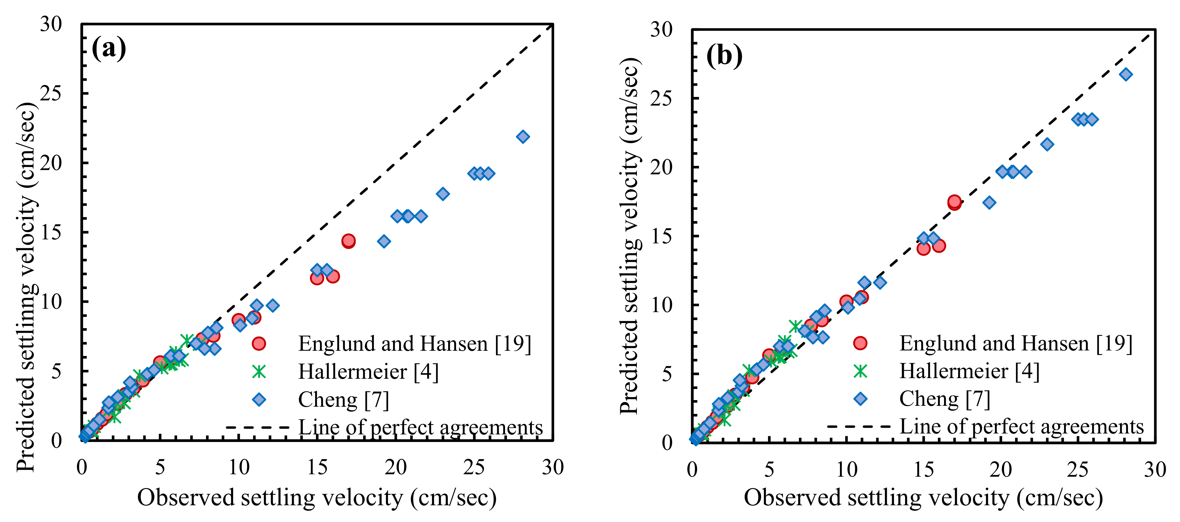
In this present study, a total of fourteen (eleven without S_f; three with S_f) equations proposed by earlier investigators [2,3,5,6,7,8,9,10,12,15,16] were checked with 226 field and laboratory experimental data sets [4,7,19,20,24]. The accuracy and reliability of these equations were analysed both graphically and statistically. In Figure 1a–k and Figure 2a–c, values on X-axis and Y-axis represent the observed and predicted data sets of the settling velocity of particles, respectively. The data set has been divided into two groups: one is without the shape factor (assumed as a natural particle, S_f = 0.7); the second is with the shape factor (shape factor considered explicitly). The first group consists of data sets of Engelund and Hansen [19], Hallermeier [4], and Cheng [7]. The second group consists of the data sets of Briggs [24] and Raudkivi [20].

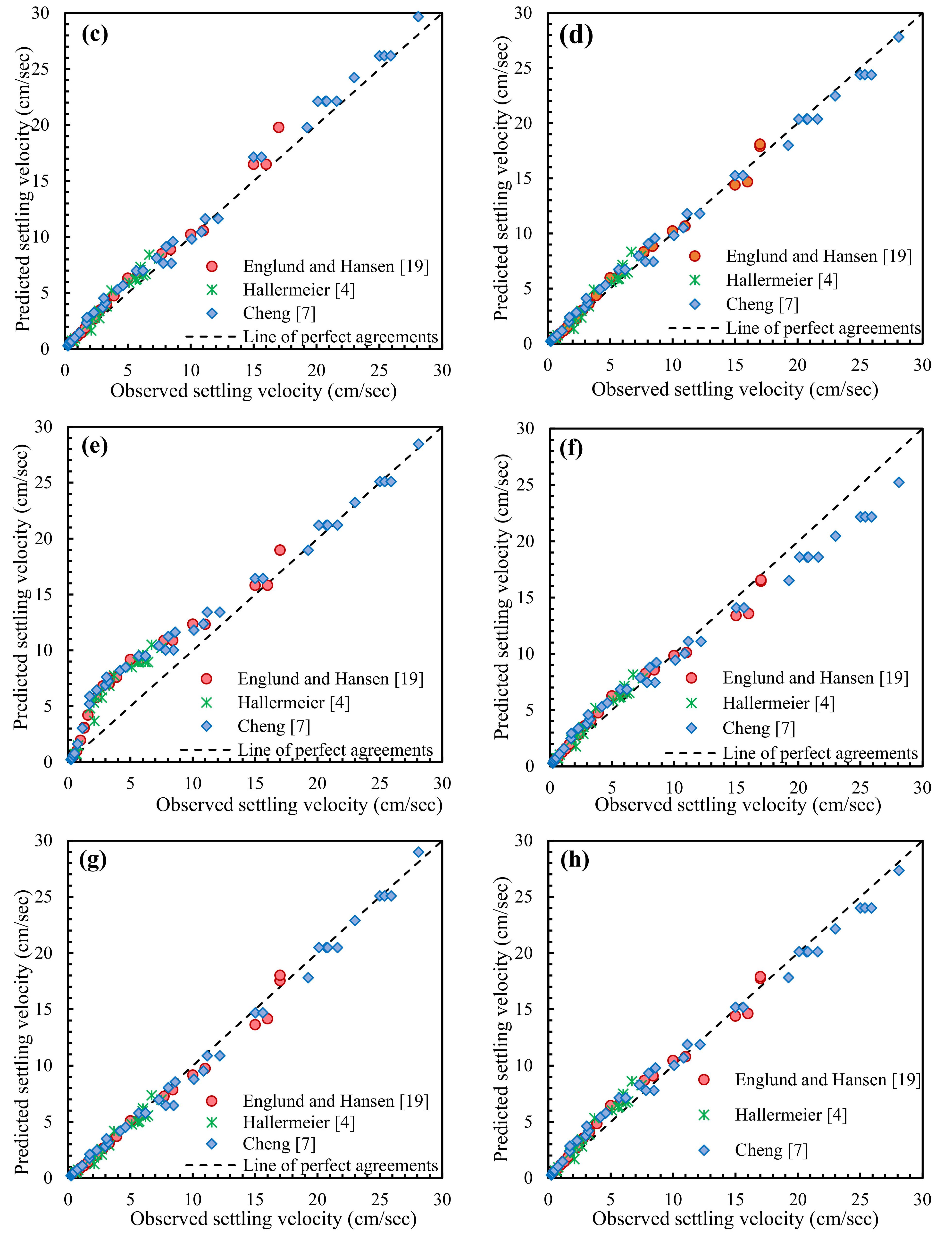
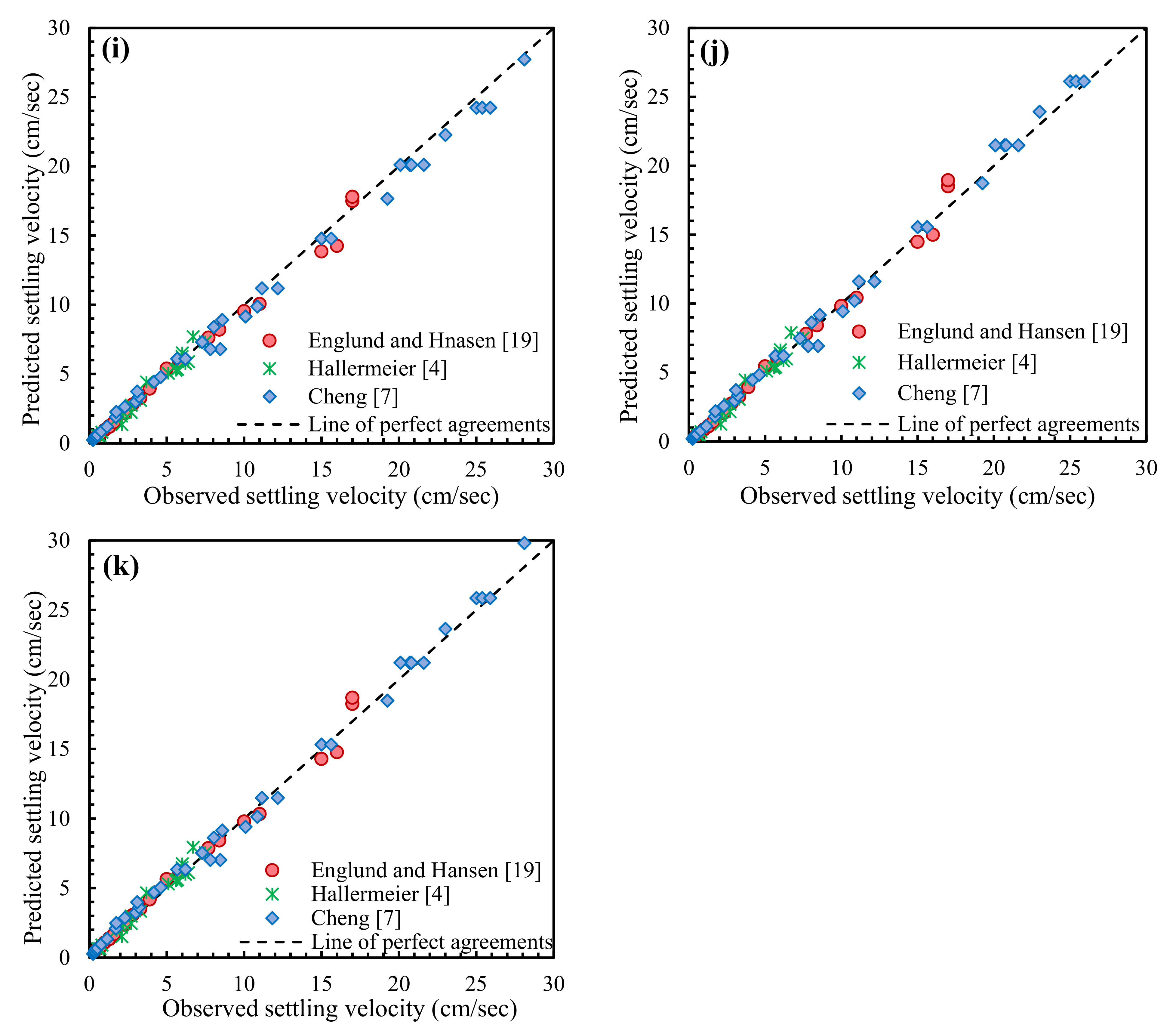
Figure 1i,k are the graphical representation of the observed and predicted data by the equations of Jimenez and Madsen [8] and Camenen [16] without the shape factor. Results show that the equations of both Jimenez and Madsen [8] and Camenen [16] performed well and produced nearly the same results for fine sediments (lower settling velocity); in the case of coarse sediments (higher settling velocity), these equations performed slightly under prediction and over prediction, respectively. There is a limitation for Jimenez and Madsen’s [8] equation, as it was developed for a certain diameter range (0.63 mm–1 mm).

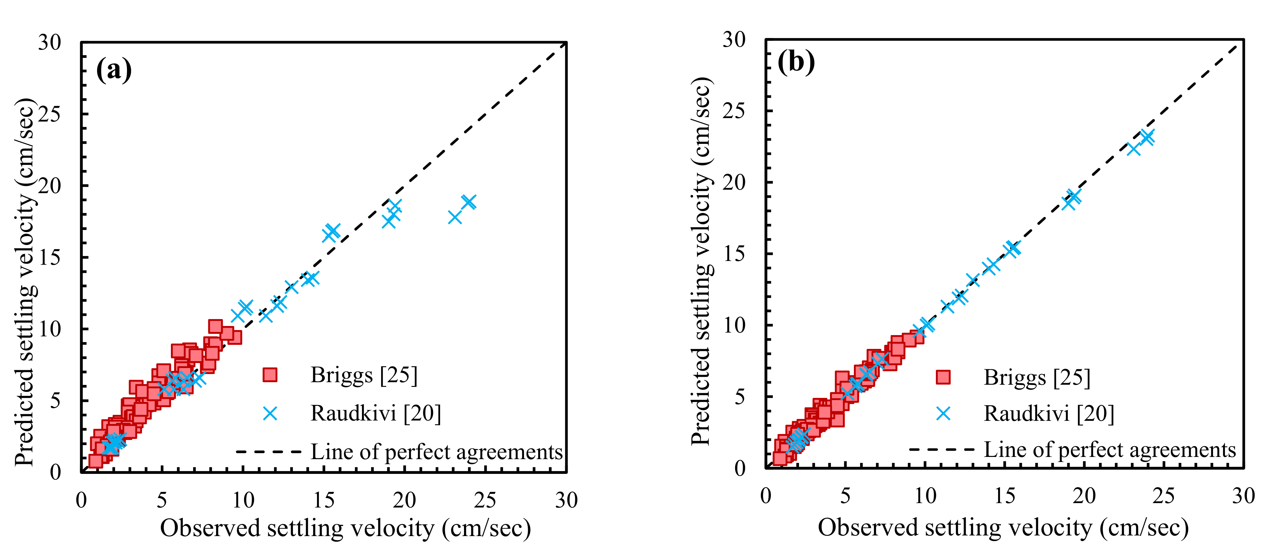
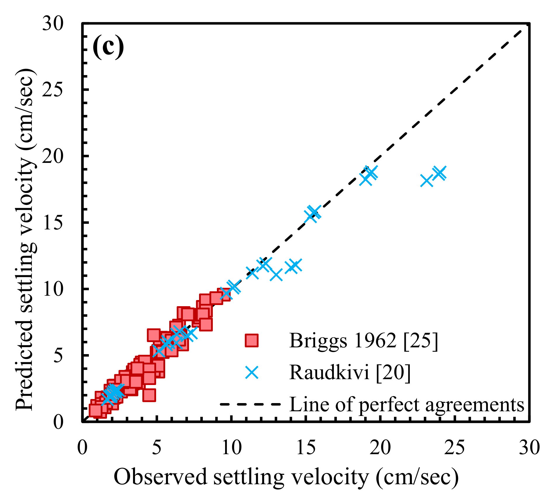
The equation of Cheng [7] also showed good agreement with the observed data without the shape factor (natural sediment particles, i.e., S_f assumed as 0.7), and a slight under prediction is observed through scatter plot 1(g). Zhang’s [9] expression was over predicted for lower settling velocity between 2–9 cm/s and further observed good agreement with measured settling velocity data, shown in Figure 1d. The agreement between observed and predicted data of Zanke [3], Soulsby [12], and Julien [10] expressions are shown in Figure 1b,f,h, respectively. Due to similarities between equations, these three expressions show analogous trends in their scatter plots, and Julien’s [10] equation showed lower accuracy graphically and statistically. Rijn [5] gave over prediction with moderate performance as shown in Figure 1c. Rijn [5] divided datasets into three sediment diameter ranges (d < 0.01 cm, d > 0.1 cm, and d = 0.01–0.1 cm) and most of the collected datasets belonged to d > 0.01 cm, which may be the reason for over prediction with moderate performance. Figure 1j and Figure 2b show the agreement between observed and predicted settling velocity by the equation of Wu and Wang [15], with and without the shape factor, respectively. Wu and Wang [15] included the importance of the shape factor and excluded the particle roundness factor. This was done so that it could be used only for data that excludes the roundness factor; if not, an error in the particle’s settling velocity calculations could occur.

Most of the data showed incredibly good agreement graphically and statistically because of a simple equation that explicitly included the effect of the shape factor. Camenen’s [16] expression with the inclusion of the shape factor produced a low agreement with the observed data, which can be seen in Figure 2c. It would have been shown to be in good agreement when the shape factor is considered; however, the results showed low agreement because of the complex equation and insufficient data of all parameters. The expression of Jimenez and Madsen [8] with the shape factor showed poor agreement compared with the above mentioned equations for these data sets. The equations of Ruby [2] and Zhu and Cheng [6] showed extremely poor agreement with the observed data with under and over prediction, respectively.

In computing the settling velocity of sediment particles, the authors observed that the equation proposed by Wu and Wang [15] (with and without shape factor) illustrates better agreement with the predicted and observed data than the others. However, the reason for the poor performance of Jimenez and Madsen’s [8] and Camenen’s [16] equations with shape factors may be due to the complexity of their equations and inadequate data sets.

4.2. Statistical Performance Analysis of Equations

A statistical analysis was also done to check the accuracy of these equations. Five statistical indices were taken to enhance the agreement between the predicted and observed settling velocity of sediment particles with and without shape factor. If M is the measured (or observed) value and P is the corresponding predicted (or computed) value, the various performance indices are defined as shown in Equation (12). The co-efficient of determination (R²) explains the fraction of total variance in observed data sets, and it ranges from 0 to 1:

$$R^2=\frac{{{\displaystyle \sum }}_{i=1}^n\left(M_i-\overline{M}\right)(P_i-\overline{P)}}{\sqrt{{{\displaystyle \sum }}_{i=1}^n{\left(M_i-\overline{M}\right)}^2}\sqrt{{{\displaystyle \sum }}_{i=1}^n{\left(P_i-\overline{P}\right)}^2}}$$

(21)

where, $M_i$ = Observed data, $P_i$ = Predicted data, $\overline{M}$ = mean of observed data, and $\overline{P}$ = mean of predicted data.

Nash–Sutcliffe efficiency (NSE) is the most extensively used index. It represents the absolute difference between measured and predicted data, which is then normalized with the measured variance. The range exists between −∞ and 1, with 1 representing the perfect fit.

$$E=1-\frac{{{\displaystyle \sum }}_{i=1}^n{\left(M_i-P_i\right)}^2}{{{\displaystyle \sum }}_{i=1}^n{\left(M_i-\overline{M}\right)}^2}$$

(22)

Kling–Gupta efficiency (KGE)

$$E=1-ED$$

(23)

ED is calculated as,

$$ED=\sqrt{{\left(r-1\right)}^2+{\left(\frac{{\sigma }_p}{{\sigma }_m}-1\right)}^2+{\left(\frac{{\mu }_p}{{\mu }_m}-1\right)}^2}$$

(24)

where; ED = Euclidian distance from the ideal point, r = linear correlation coefficient between predicted and observed data, ${\sigma }_p$,${\sigma }_m$ = standard deviation of predicted and observed data, respectively, and ${\mu }_p$, ${\mu }_m$ = mean of predicted and observed data, respectively.

Percent bias (PBIAS) represents the average deviation in percentage of the predicted data from the observed data.

$$PBIAS=\frac{{{\displaystyle \sum }}_{i=1}^n\left(M_i-P_i\right)}{{{\displaystyle \sum }}_{i=1}^n{M}_i}\times 100$$

(25)

Mean Absolute Error (MAE):

$$MAE=\frac{1}{n}{\displaystyle \sum }_{i=1}^n\left|\left(M_i-P_i\right)\right|$$

(26)

In Equations (21)–(26), n is the number of data sets, i.e., 226. Values of R², NSE, KGE, PBIAS, and MAE for different equations are listed in

Table 2. Statistical values.

Researchers	NSE	KGE	PBIAS	MAE	R2
Wu and Wang [15] with Sf	0.9937	0.976	−1.06	0.2691	0.9942
Wu and Wang [15] without Sf	0.9931	0.9616	−1.463	0.4107	0.9948
Camenen [16] without Sf	0.9936	0.9733	−2.3895	0.4376	0.9944
Jimenez and Madsen [8] without Sf	0.9929	0.9512	2.6308	0.4164	0.9952
Cheng [7] without Sf	0.9924	0.96	3.8275	0.4342	0.9941
Zhang [9] without Sf	0.9925	0.964	−1.7206	0.4835	0.9937
Zanke [3] without Sf	0.9847	0.9143	−2.4174	0.7276	0.9914
Soulsby [12] without Sf	0.9861	0.9241	−4.5574	0.7057	0.9915
Rijn [5] without Sf	0.9824	0.8998	−9.1874	0.7705	0.9933
Camenen [16] with Sf	0.9581	0.8958	3.4168	0.5018	0.9661
Julien [10] without Sf	0.9714	0.8582	1.0309	0.9229	0.9901
Jimenez and Madsen [8] with Sf	0.9234	0.8648	−6.1132	0.8406	0.9354
Ruby [2] without Sf	0.9069	0.7104	12.4768	1.3657	0.989
Zhu and Cheng [6] without Sf	0.8707	0.7057	−28.4017	2.1954	0.9599

. The R², NSE, and KGE of Equation (14), i.e., proposed by Wu and Wang [15], are highest, and PBIAS and MAE are lowest among all other equations. Statistical performances indicate that the expression of Wu and Wang [15] predicts the better settling velocity of sediment particles than all other equations. This was observed graphically and statistically. The expressions proposed by Camenen [16] and Jimenez and Madsen [8] without the shape factor provided the second highest agreements between observed and predicted data, as can be seen in Table 2 and Figure 1.

5. Conclusions

The present study describes the settling velocity phenomenon and deals with the methods for its estimation. A total of fourteen equations (eleven without S_f; three with S_f) were used for verifying the accuracy and performance of particle settling velocity. The authors graphically observed that the relationship proposed by Wu and Wang [15], with and without the shape factor, provides superior agreements, as is shown in Figure 1j and Figure 2b. Statistically, the relationships proposed by Wu and Wang [15], with and without the shape factor, and Camenen [16], Jimenez and Madsen [8], and Cheng [7], without the shape factor, provide approximately similar values among all. However, Wu and Wang [15] show slightly higher values than the other equations, as shown in Table 2. Graphically and statistically, it was observed that the expressions of Zanke [3], Soulsby [12], and Julien [10] show the same pattern with medium performance. The low performance of Jimenez and Madsen’s [8] and Camenen’s [16] equations may be strictly due to particular datasets. There may be a scope for checking the accuracy of the above equations with broad datasets, including particle shape factor and roundness factor.

Finally, it was determined by the authors after graphical and statistical investigations that the expression proposed by Wu and Wang [15] predicts the settling velocity of sediment particles both with and without the shape factor cases, showing the least errors among all equations. Hence, the present study highlights that Wu and Wang’s [15] equation predicts the accurate value of settling velocity of a particle.

References

- Gibbs, R.J.; Matthews, M.D.; Link, D.A. The relationship between sphere size and settling velocity. J. Sediment. Res. 1971, 41, 7–18. [Google Scholar]
- Ruby, W. Settling velocities of gravel, sand and silt particles. Am. J. Sci. 1933, 25, 325–338. [Google Scholar] [CrossRef]
- Zanke, U. Berechnung der Sinkgeschwindigkeiten von Sedimenten; Heft 46, Seite 243; Franzius-Institut für Wasserbau und Küsteningenieurwesen: Hannover, Germany, 1977. [Google Scholar]
- Hallermeier, R.J. Terminal settling velocity of commonly occurring sand grains. Sedimentology 1981, 28, 859–865. [Google Scholar] [CrossRef]
- Rijn, L.C.V. Sediment transport, part II: Suspended load transport. J. Hydraul. Eng. 1984, 110, 1613–1641. [Google Scholar] [CrossRef]
- Zhu, L.J.; Cheng, N.S. Settlement of Sediment Particles; Resp. Rep., Dept of River and Harbor Eng. Nanjing Hydr. Res. Inst.: Nanjing, China, 1993. (In Chinese) [Google Scholar]
- Cheng, N.S. Simplified Settling Velocity Formula for Sediment Particle. J. Hydraul. Eng. 1997, 123, 149–152. [Google Scholar] [CrossRef]
- Jiménez, J.A.; Madsen, O.S. A simple formula to estimate settling velocity of natural sediments. J. Waterw. Port Coast. Ocean Eng. 2003, 129, 70–78. [Google Scholar] [CrossRef] [Green Version]
- Zhang, R.J. River Dynamics; Industry Press: Beijing, China, 1961. (In Chinese) [Google Scholar]
- Julien, P.Y. Erosion and Sedimentation; Cambridge University Press: Cambridge, UK, 2010. [Google Scholar]
- Pandey, M.; Sharma, P.K.; Ahmad, Z.; Singh, U.K.; Karna, N. Three-dimensional velocity measurements around bridge piers in gravel bed. Mar. Georesour. Geotechnol. 2018, 36, 663–676. [Google Scholar] [CrossRef]
- Soulsby, R. Dynamics of Marine Sands: A Manual for Practical Applications; Thomas Telford: Telford, UK, 1997. [Google Scholar]
- Pourshahbaz, H.; Abbasi, S.; Pandey, M.; Pu, J.H.; Taghvaei, P.; Tofangdar, N. Morphology and hydrodynamics numerical simulation around groynes. ISH J. Hydraul. Eng. 2020, 1–9. [Google Scholar] [CrossRef]
- Ahrens, J.P. A fall-velocity equation. J. Waterw. Port Coast. Ocean Eng. 2000, 126, 99–102. [Google Scholar] [CrossRef]
- Wu, W.; Wang, S.S. Formulas for sediment porosity and settling velocity. J. Hydraul. Eng. 2006, 132, 858–862. [Google Scholar] [CrossRef]
- Camenen, B. Simple and general formula for the settling velocity of particles. J. Hydraul. Eng. 2007, 133, 229–233. [Google Scholar] [CrossRef]
- Stokes, G.G. On the effect of the internal friction of fluids on the motion of pendulums. Trans. Camb. Phil. Soc. 1851, 9, 8–106. [Google Scholar]
- Dietrich, W.E. Settling velocity of natural particles. Water Resour. Res. 1982, 18, 1615–1626. [Google Scholar] [CrossRef]
- Engelund, F.; Hansen, E. A Monograph on Sediment Transport in Alluvial Streams; Technical University of Denmark: Copenhagen, Denmark, 1967. [Google Scholar]
- Raudkivi, A.J. Loose Boundary Hydraulics, 3rd ed.; Technical report; Pergamon Press: Oxford, UK, 1990. [Google Scholar]
- Zegzhda, A.P. Settlement of Sand Gravel Particles in Still Water; Izv. NIIG, 12; Moscow, Russia, 1934. (In Russian) [Google Scholar]
- Arkangel’skii, B.V. Experimental Study of Accuracy of Hydraulic Coarseness Scale of Particles; Isv. NHG, 15; 1935. [Google Scholar]
- Sarkisyan, A.A. Deposition of Sediment in a Turbulent Stream; Izd. AN SSSR: Moscow, Russia, 1958. (In Russian) [Google Scholar]
- Briggs, L.I.; McCulloch, D.S.; Moser, F. The hydraulic shape of sand particles. J. Sediment. Res. 1962, 32, 645–656. [Google Scholar]
- Amit, K.; Sharma, M.P.; Rai, S.P. A novel approach for river health assessment of Chambal using fuzzy modeling, India. Desalination Water Treat. 2017, 58, 72–79. [Google Scholar]
- Pandey, M.; Lam, W.H.; Cui, Y.; Khan, M.A.; Singh, U.K.; Ahmad, Z. Scour around Spur Dike in Sand–Gravel Mixture Bed. Water 2019, 11, 1417. [Google Scholar] [CrossRef] [Green Version]
- Kumar, A.; Cabral-Pinto, M.; Kumar, M.; Dinis, P.A. Estimation of risk to the eco-environment and human health of using heavy metals in the Uttarakhand Himalaya, India. Appl. Sci. 2020, 10, 7078. [Google Scholar] [CrossRef]
- Singh, R.K.; Pandey, M.; Pu, J.H.; Pasupuleti, S.; Villuri, V.G.K. Experimental study of clear-water contraction scour. Water Supply 2020, 20, 943–952. [Google Scholar] [CrossRef]
- Kumar, A.; Mishra, S.; Taxak, A.K.; Pandey, R.; Yu, Z.G. Nature rejuvenation: Long-term (1989–2016) vs short-term memory approach based appraisal of water quality of the upper part of Ganga River, India. Environ. Technol. Innov. 2020, 20, 101164. [Google Scholar] [CrossRef] [PubMed]
- Singh, U.K.; Ahmad, Z.; Kumar, A.; Pandey, M. Incipient motion for gravel particles in cohesionless sediment mixtures. Iran. J. Sci. Technol. Trans. Civ. Eng. 2019, 43, 253–262. [Google Scholar] [CrossRef]
- Mishra, S.; Kumar, A.; Shukla, P. Estimation of heavy metal contamination in the Hindon River, India: An environmetric approach. Appl. Water Sci. 2021, 11, 2. [Google Scholar] [CrossRef]
- Singh, P.; Kumar, A.; Mishra, S. Performance evaluation of conservation plan for freshwater lakes in India through a scoring methodology. Environ. Dev. Sustain. 2021, 23, 3787–3810. [Google Scholar] [CrossRef]
Figure 1.
(a–j) Observed versus predicted settling velocity without shape factor using: (a) Ruby [2]; (b) Zanke [3]; (c) Rijn [5]; (d) Zhang [9]; (e) Zhu and Cheng [6]; (f) Julien [10]; (g) Cheng [7]; (h) Soulsby [12]; (i) Jimenez and Madsen [8]; (j) Wu and Wang [15]; and (k) Camenen [16].
Figure 2.
(a–c) Observed versus predicted settling velocity with shape factor using: (a) Jimenez and Madsen [8]; (b) Wu and Wang [15]; and (c) Camenen [16].