Article

Silting in the Grand Canal in the Domain of Chantilly (Oise, France)—Catchment-Scale Hydrogeomorphological Reconnaissance and Local-Scale Hydro-Sedimentary Transport Modelling

ULR 4477, TVES–Territoires Villes Environnement & Société, University Lille, University Littoral Côte d’Opale, F-59000 Lille, France
*
Author to whom correspondence should be addressed.
Water 2021, 13(14), 1989; https://doi.org/10.3390/w13141989
Submission received: 12 May 2021 / Revised: 11 July 2021 / Accepted: 14 July 2021 / Published: 20 July 2021
(This article belongs to the Special Issue Fluvial Hydraulics and Applications)

Abstract

:
The domain of Chantilly (Oise, France) includes a castle and a garden, both dating from the eighteenth century, which are seen as important legacies of France’s history. Nowadays, the 2.5 km canal that runs through the domain is subject to the phenomenon of silting, leading to the accumulation of sediments within the canal linked to the proliferation of algae, which has a dissuasive effect among visitors. HEC-RAS software (Hydrologic Engineering Centers River Analysis System, US army corps of Engineers, Washington, D.C., USA) was used to model and understand sediment accumulation within the canal. This model is widely used in the literature tackling sediment transport and accumulation, and allows the forecasting of which stretches of the canal are most susceptible to sediment accumulation. The simulation results highlight an accumulation of sediment near the entrance of the Nonette stream into the canal and a propagation through the canal. The total accumulated volume assessed by the model between 2001 and 2010 equals 3901 m3, when the reconnaissance of the catchment showed the sediment was not a limiting factor. However, the volumes determined are underestimated, as matter brought by vegetation or other systems different from the river (e.g., wind, rainfall) is not considered in the calculation. The quantity of sediment is also subject to uncertainties, as the bathymetry of the canal is not available.

1. Introduction

Many European castles with parkland and artificial water features, such as canals, moats and water mirrors, have been affected by sediment accumulation for centuries, as well as in recent decades. Dredging and maintenance operations for these small infrastructures cannot benefit from the costs negotiated for the extraction of very large volumes of sediments, such as those contained in seaports, river ports and waterways, which also benefit from proportionally higher operating revenues than those of tourist castles. The modelling of sediment flows and sedimentation rates in the aquatic infrastructures of castles is essential knowledge for the implementation of management plans for these infrastructures. Many castles are connected to rivers by discharge arms to take the necessary quantities of water, to maintain the water levels in their hydraulic infrastructures.
The domain of Chantilly (Oise, France) is made up of a castle and a garden. The castle was completely rebuilt during the nineteenth century and the Grand Canal (GC), which is the masterpiece of the garden, is one of the few infrastructures that has not undergone any changes. Preserving this historical heritage is of the utmost importance for Chantilly Castle’s conservation. As a matter of fact, the GC is the longest canal dating from this period, even surpassing the one from Versailles Castle in length. Nowadays, the GC greatly contributes to Chantilly’s tourism and therefore contributes to Chantilly’s economics. For the past several years, the Chantilly estate manager has reported that the canal problems have been attributed to a loss of income due to aesthetic impact. The quantity of sediment in the canal has increased and the proliferation of algae during the summer period has decreased the quality of the boat-rowing experience. The problem of the algae’s uncontrolled growth also impacts on an annual sporting event, which takes place at the end of August every year. The triathlon is part of a series of events involving several castles across north-western Europe. Turbid waters and algae growth devalue the sporting conditions of the Chantilly event. This has contributed to a reduction in the number of registrations for the triathlon, as the manager of the triathlon told the authors, and therefore, is an additional loss of income for the castle. The loss of income from tourists and in relation to activities on the canal is a problem for the maintenance of the domain, whose overall budget is difficult to balance. Additionally, the cost of dredging the canal is a problem that cannot be compensated by the income from visits to the domain alone.
In order to report the behaviour of sediment accumulation in the GC in the domain of Chantilly, it was decided to run the one-dimensional (1D) Hydrologic Engineering Center’s River Analysis System (HEC-RAS model) [1]. One-dimensional numerical models, such as 1D HEC-RAS, are easily implementable as (1) the calculations involved are comparatively simple, (2) calibration and validation require a limited amount of hydrological data and (3) they allow for fast computation [2,3].
In the literature, HEC-RAS has proven useful in diverse sediment transport studies and examples of its application are numerous [4,5,6,7]. HEC-RAS is suitable for use in a wide range of environments and permits the study of the transport of all types of sediments where little data are available.
This present article is a case study of the sediment accumulation within the GC in the domain of Chantilly. First, a reconnaissance study performed at catchment scale is proposed, based on diverse geosciences, in order to contextualize the sediment availability tackled in the second part of this article. In this second part, the geometry of the GC has been digitalized and used in the HEC-RAS model. It aims to assess the accumulation dynamics of suspended sediment (SS) and to give an order of magnitude of the quantity of accumulated sediment within the canal for the domain’s caretakers to better comprehend this issue and conduct appropriate canal maintenance works (such as dredging).

2. Hydrogeomorphological Reconnaissance at Catchment Scale

2.1. Hydrology

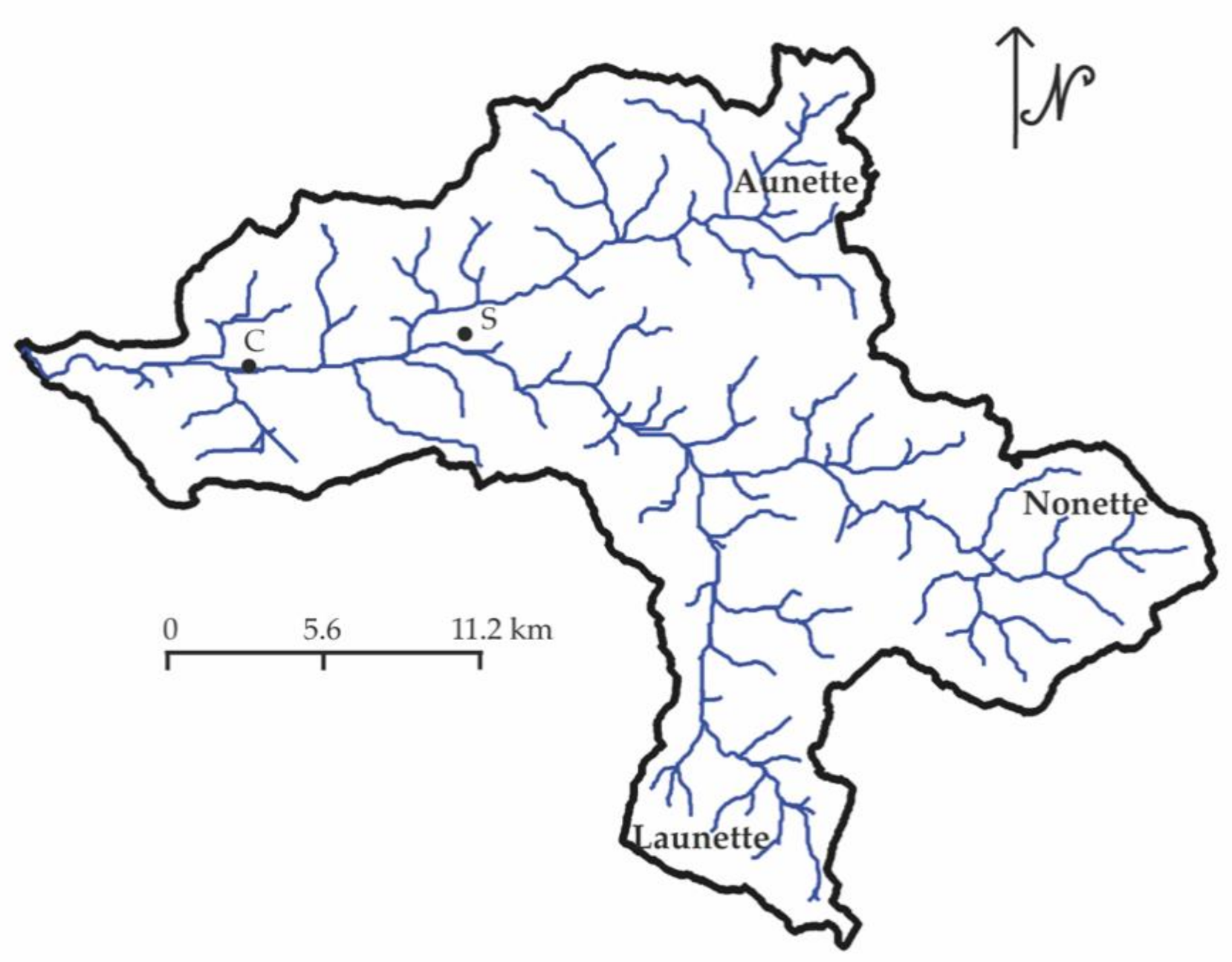
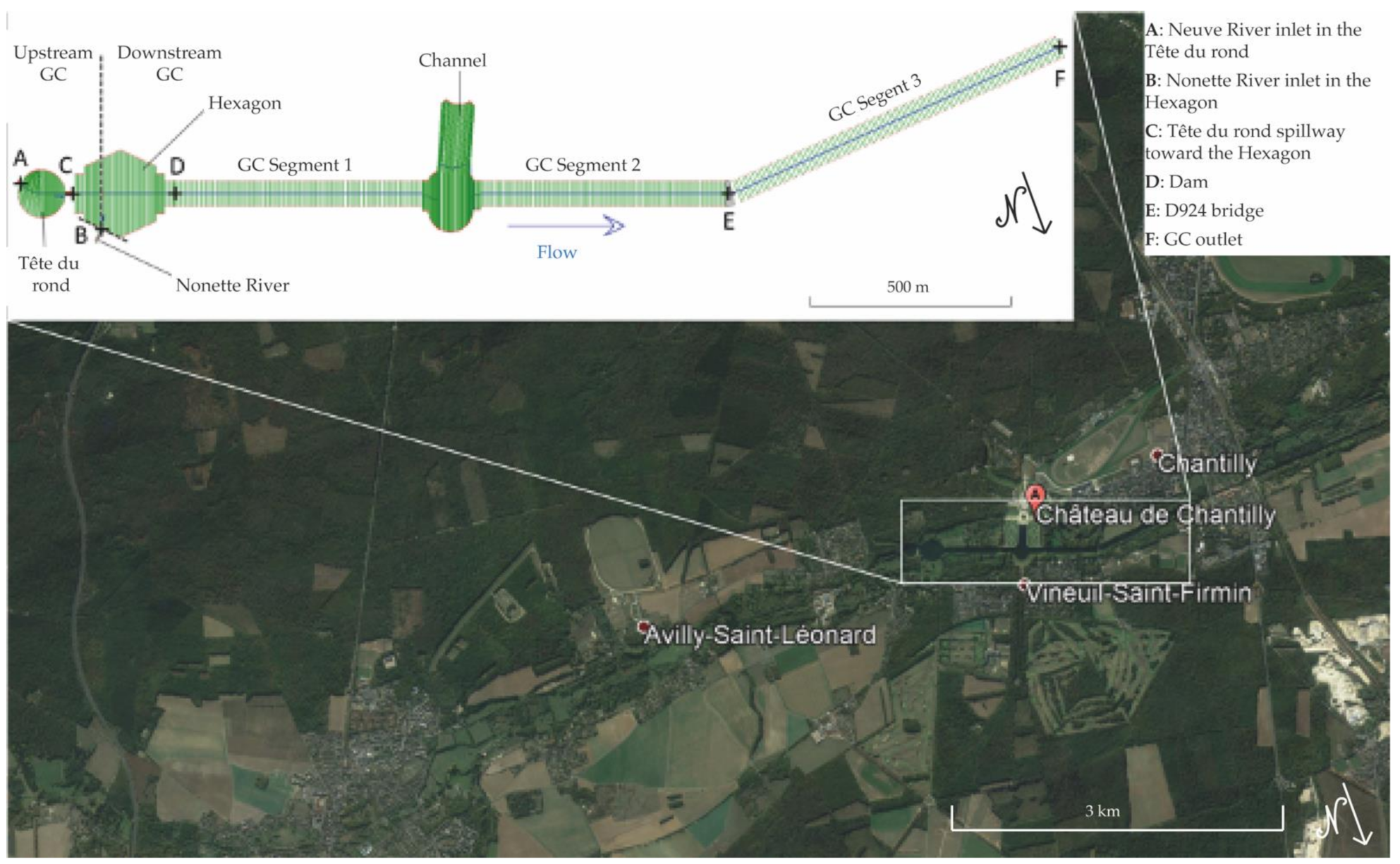
The Nonette catchment lies 40 km north of Paris and about 7 km west of Senlis. It comprises three main rivers (Nonette, Launette and Aunette (Figure 1)), which eventually flow into the Oise River.
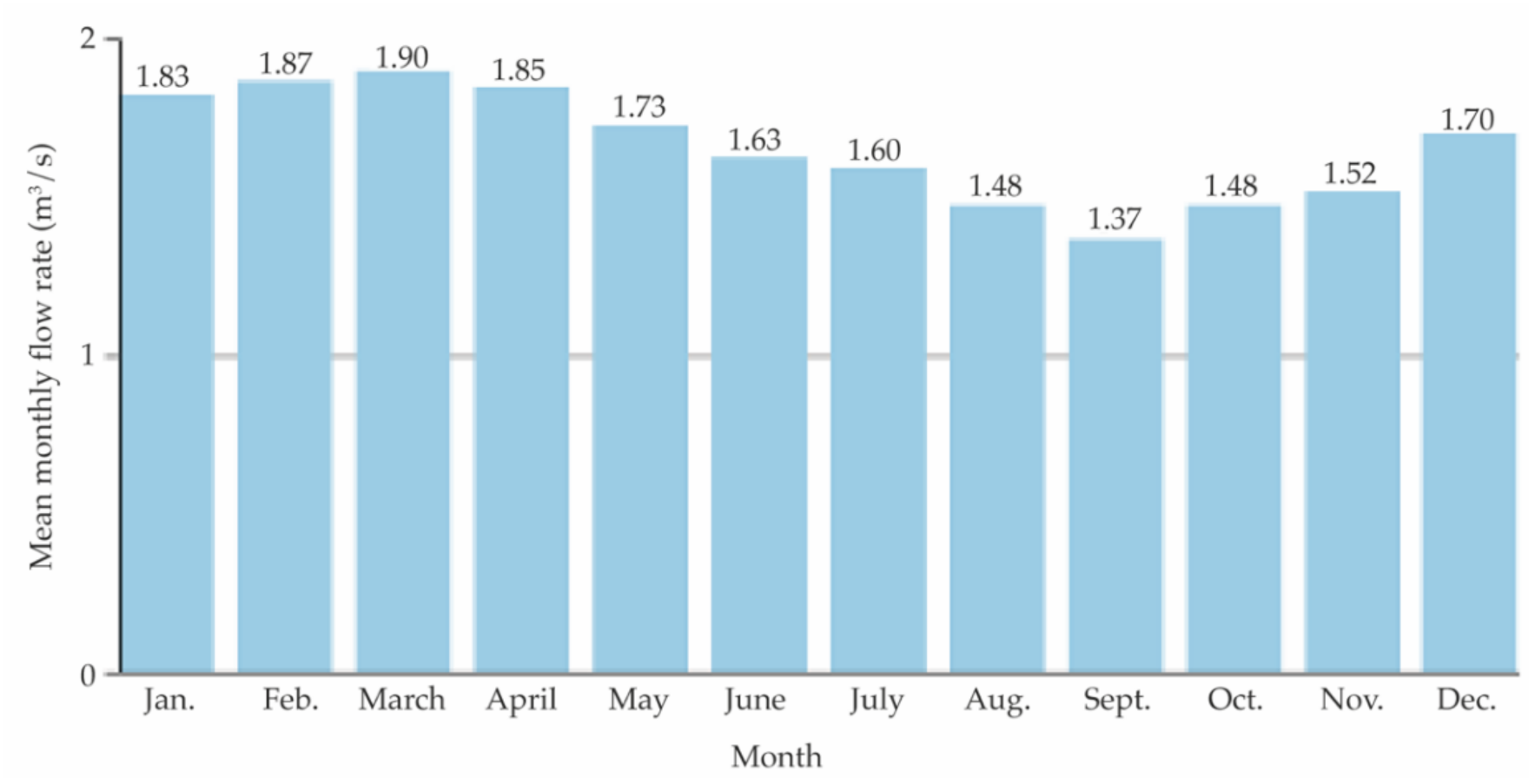
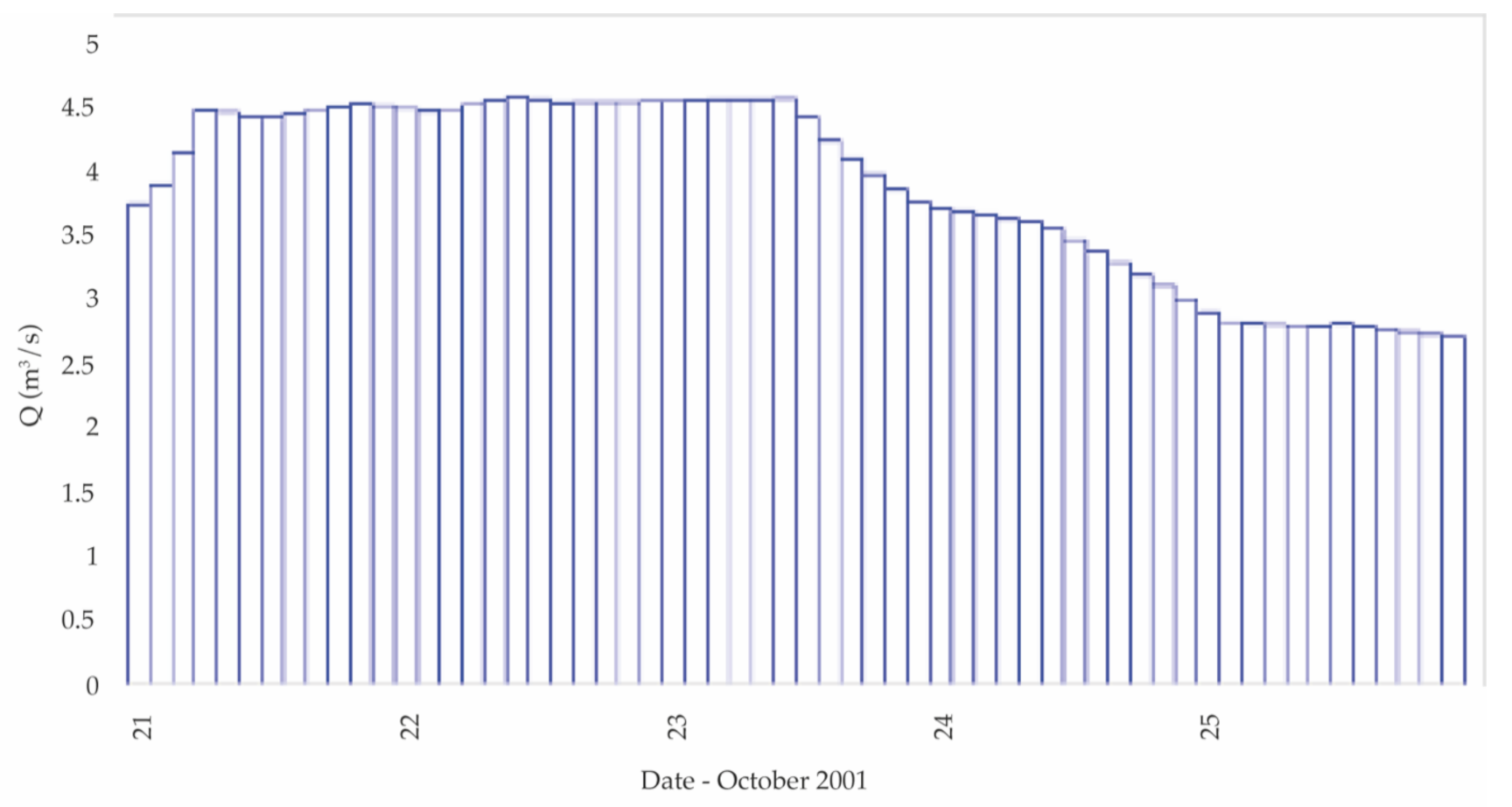
The Nonette River’s discharge has been observed for 41 years (1968–2008) at Courteuil, near its confluence with the Oise River [8] and this observation is reproduced in Figure 2. In this database, the Nonette catchment’s area is 338 km2 and the modulus of the river equals 1.66 m3/s.
Flow discharges’ seasonal fluctuations are very low, as generally observed in parts of the Seine catchment, areas near Normandy and the Somme catchment. The Nonette streamflow is fairly regular throughout the year, although the mean flow discharge is more important between December and May, with a maximum discharge in March. Starting in June, the flow discharge decreases and reaches a flat/threshold between August and October, with a minimum discharge in September.
Flooding is not factor, as each year, the probability of a 3.7 m3/s flood is 50% and the probability of a 4.2 m3/s flood is 20% (4.5 m3/s flood probability is 10%; 4.8 m3/s flood probability is 5%; and 5.3 m3/s flood probability is 2%).
The Nonette stream is not abundant, as the annual depth of runoff is 155 mm, which is very low compared to other French catchments (e.g., 240 mm for the Seine catchment). It leads to a low Qsp of 4.9 l/s/km2.
Given these data, it appears that the sediment transport is limited by the hydrological activity of the Nonette River.

2.2. Geology

The Nonette catchment belongs to the Paris basin. This basin is a typical example of an intra-cratonic basin whose subsidence has been linked to thermal subsidence due to the Permian extension [9]. There is a recorded history of this in western Europe between Trias (262–201 My) and Miocene (23–5.3 My). The study of sedimentary and tectonic records and eustatic sea level have shed light on the basin’s deep structure [9], thermal subsidence [10], intraplaque domain deformations recordings, and eustatic sea level changes [11,12,13].
Only a part of this history is relevant for the Nonette catchment, for the earlier geological units recognized there are from Ypresian, with the latest from Rupelian (Figure 3). An extensive description of the lithologies is presented in [14], and can be constrained to limestones, marls, pebbles and sands. On top of the bedrock, an assemblage of different Quaternary deposits made of alluvium, colluvium, dunes sand, clay with silex and loess and silts is found. Concerning quaternary deposits, their thicknesses are not reported, although their extents, which are presented in Figure 1, are mainly concentrated in the upper parts of the catchment.
It appears that the material making up the local geology is weak; the presence of Quaternary deposits is substantial, and therefore, sediment availability seems not to be limited by these lithologies.

2.3. Geomorphology

Based on Figure 4, the Nonette catchment’s geomorphology permits the recognition of three different units: an upper plateau, a floodplain with the riverbed, and a zone of steeper (than the two former units) slopes that represent the contact between the floodplain and the plateau. Usually, these slopes are associated with the upper surface, as between two fluvial terraces, but it was decided in this paper to distinguish between them in order to emphasize the different geomorphological units. It is to be noted that these slopes tend to create geological escarpments.
  • The plateau is found throughout the south-eastern part of the catchment, to the east, and bordering the northern boundary (in red in Figure 4a);
  • A zone of steeper slopes is where the contact between two fluvio-geomorphological units is generally found. In Figure 4b, most of the steep slopes mark the contact between the plateau and the floodplain, which are in the order of 20–25° and in orange in Figure 4a. Depending on fluvial erosion, this contact can be slightly hilly or present a (more-or-less abrupt) ridge. For instance, from Figure 4a, the southwestern edge of the contact between the plateau and the floodplain (very limited in space, so red and green are very close) and the northern part (where red and green areas are well marked with orange) are quite different; the southwestern part is not hilly (presence of ridge), whereas the northern half is;
  • The scale of Figure 4 is not realistic in distinguishing between riverbed and floodplain. Riverbed is where water is flowing unceasingly, and floodplain is water flow when the bed can no longer manage the flow. Schematically, the floodplain is visible near the outlet when the bed is not. Near headwaters, the floodplain is non-existent. This is why the river seems to be made up of minute streams in the headwaters and larger ones near its outlet. The contact between the zone of steeper slopes and floodplain is again interpreted as following another set of steep slopes, this time more or less following the river. Additionally, at a local scale, the presence of fluvial terraces along the river is likely (although invisible in Figure 4, due to the scale).
The presence of a zone of steep slopes is an argument in favour of a source of sediment capable of covering the soil and merging with river transport, with consequences in terms of excess sedimentation within the territory, as seen in the GC.

2.4. Morphometry

Morphometrical data of the Nonette catchment presented in Table 1, is obtained thanks to the digital elevation model (from which the slope raster was also determined) provided [15], which expresses the landscape with a 25 m resolution, and the use of the Spatial Analyst tool (zonal statistics as table and zonal geometry as table) of ArcGIS 10.7 (ESRI, Redlands, CA, USA) [16].
Table 1 highlights the parameters gathered by the GIS together with units, equations and the entity to which the parameters have been determined. Area, perimeter, maximum, minimum and mean elevation, mean slope, length, Melton ratio, form factor and basin elongation constitute these parameters.
The Nonette catchment is a fourth-order catchment when using Strahler’s ordination system [17]. The catchment’s area is equal to 393 square kilometres (km2) with a perimeter of 138 km. The catchment’s minimum elevation equates to 25 m above sea level (m asl) near Gouvieux and the maximum elevation reaches 222 m asl (mean elevation equal to 93 m asl). Concerning slopes, a mean value of 1.66 degrees (°) was found, with the maximum value reaching 29.7°.
The Nonette stream has also been studied following the same logic used for the catchment. Its length is 279 km. The maximum elevation is 222 m asl; the mean elevation is 93 m asl; and the minimum elevation is 25 m asl. The mean slope equates to 1.66° with a maximum of 29.69°.
Moreover, it has been possible to determine a series of fluvial ratios (Table 1), able to characterize the hydrological surface and behaviour of catchments: the Melton ratio, form factor and basin elongation. The Melton ratio is an index of a surface’s rugosity. The higher the ratio, the higher the surface’s rugosity. For the Nonette catchment, this value equates to 0.01; the rugosity of the catchment is low; therefore, the catchment is rather smooth and flat. Form factor and basin elongation both allow the apprehension of fluvial dynamics. Form factor, which cannot be attributed a greater value than 0.7854 in the case of a perfectly circular catchment, expresses the roundness of a catchment. Catchments with a form factor value approaching zero (0) account for elongated catchments; catchments with a form factor value approaching 0.7854 account for circular catchments. In terms of fluvial dynamics, the shape of a catchment influences the shape of the hydrograph at its outlet. For a given amount of rainfall, an elongated shape tends to create low peak discharge. The Nonette catchment’s form factor equates to 0.5; the Nonette catchment is rather circular. Peak discharge is important given the little time required for the water to travel to the outlet.
In a GIS environment, the hydrographical network has been divided as proposed by [17]; first-order, second-order, third-order and fourth-order catchments have been determined. The same series of parameters, as mentioned above, have been gathered for each catchment and stream (Table 1). The results are proposed in the following Table 2, Table 3 and Table 4.
Regarding the 26 second-order catchments, the area’s mean value equates to 9.4 km2. And the perimeter is 18.1 km.
From Table 2 and concerning the 122 first-order catchments, the average first-order catchment is 2.3 km2, with a perimeter of 9.2 km. The crest line peaks at 127 m asl and the outlet is to be found 50 m lower (almost 77 m asl). This composite catchment has no slope greater than 10.6° and the mean slope over the whole catchment is 1.7°.
The elevation spans from (maximum to minimum) 147.9 to 70.6 m asl. The slope’s maximum does not exceed 4° and the mean value is less than 1°.
The four third-order catchments have an area mean value of 70.6 km2 and a perimeter of 57.8 km. The mean maximum and minimum elevations are, respectively, 173 and 53 m asl. The maximum slope reaches 18° and the mean slope is equal to 2°.
Table 3 addresses the streams found within each sub-catchment. On average, a first-order stream is 385 m long, whereas a second-order stream is 5.9 km long and a third-order stream is almost 50 km (49.6).
A first-order stream flows from 86 to 76.6 m asl (with a mean elevation of 81.2 m asl). It has no slope greater than 2.53° (mean value closing 1°) and at the outlet the slope is on average 0.17°.
A second-order stream starts at 95 m asl and the outlet is found at 70.6 m asl (the mean value of 82.3 m asl). This stream has no maximum slope greater than 4°, with a mean value approaching 1° (0.93°).
A third-order stream initiates at 110 m asl and its outlet is found at 53 m asl (with a mean value of 80 m asl). No portion of the stream has a slope greater than 9° and the mean slope along the stream is 1°.
Table 4 highlights three morpho-fluvial ratios associated with catchments.
Regarding the Melton ratio, a trend appears: value decreases as order increases. As order increases, the catchments become less steep and smoother (flatter). This behaviour is typically recognized in other networks. However, it is to be noted that the values are very low.
Concerning the form factor, it appears that first-order catchment values span the whole range of values and as the order increases, the range diminishes. First-order catchments can be quite different from one catchment to another, ranging from a rather rounded shape to a rather elongated shape, while third-order catchments are overall slightly rounded. It should be noted that mean values of form factor are close between orders.
The basin elongation acts in the same way as the two aforementioned ratios: the range of values decreases with increasing order, highlighting another constraint on the catchments’ shape as the order increases (less variability of shape for high-order catchments).
The form factor is a revealing factor that is often overlooked in erosion-related investigations. In the case of the Nonette catchment, it appears that the morphometric heterogeneity of the basins does not explain past flooding on the scale of fourth-order catchments. That being said, on the scale of first-order catchments, this heterogeneity indicates the presence of catchments where such morphometric characteristics could explain past flood episodes. Indeed, a round shape (a form factor close to the maximum, i.e., 0.750) favours flood dynamics. In other words, first-order catchments show a predisposition to flooding, while the fourth-order basin tends to lose this predisposition. Past flood events as experienced by local communities would not be related to the shape of the basin.

2.5. Climatology

The climate of Chantilly is similar to the southern Hauts-de-France region. It is best described as a mixture of an oceanic climate and continental climate. Rainfall is generally relatively light (under 700 millimetres per year), but heavy rainfall is not scarce in the spring and autumn, a common situation for oceanic climates. The continental climate is represented by stormy conditions of a continental variety.
Average temperatures are typical of oceanic climates, with temperatures increasing from winter to summer and decreasing from summer to winter [18]. The annual average high temperature reaches 15.2 °C and the average low reaches 6.7 °C.
Winds are typical of oceanic climates, with a strong SW–NE component (wind coming from the Atlantic Ocean). In terms of velocity, winds are stronger in the winter and are at their minimum during the summer.
The average wind direction generally follows the direction of flow of the Nonette River in its upstream segment, which can have an influence on the transportation of its sediments by “stimulating” it, whether the transport is by river or wind.
Based on meteoblue.com data, it appears that there are interesting directions in the prevailing winds when compared to the course of the streams in the Nonette catchment. In fact, the wind and river directions in the southern part of the basin are very close, and the same observation can be transposed to the north-western part of the same basin. The consequence is that the directions of the movement of water and of eroded material are combined, which could tend to exacerbate this transport.

2.6. Soil Use

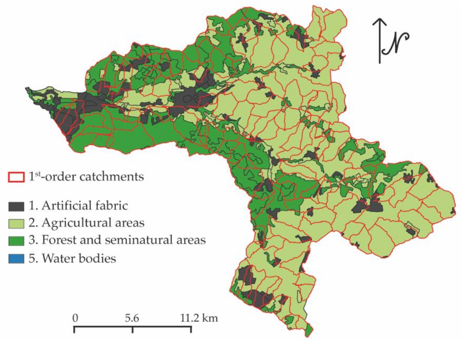
To study the soil use of the Nonette’s first-order catchments, the Corine land cover (CLC) [19] was compared to the first-order catchments’ polygons (Figure 5) and statistics were extracted.
It appears that the 122 first-order catchments comprise a total of 17 different CLC classes, which can be found in Table 5. The choice to constrain the soil use analysis to first-order catchments only is driven by the fact that these surfaces are more likely to have a low anthropogenic development (historically, places of agriculture, as opposed to urbanism) and are hotspots for surficial erosion. Moreover, the total surficial extent of these catchments accounts for 73% of the total area of the Nonette catchment.
Regarding Table 5, it can be said that on average, a first-order catchment in the Nonette catchment is covered by 10% artificial surfaces, 56.6% agricultural areas, and 35.11% forest and seminatural areas.
On the scale of the (fourth-order) Nonette catchment, the percentages of soil cover vary only slightly. In fact, the class of artificial areas covers a total of 10.5%, with agricultural areas covering 58.1% and forest and semi-natural areas covering 31.4%. It should be noted that the CLC provides information on a small area, classified as a body of water, at the confluence with the Oise, which is, however, negligible in terms of area occupied (0.005%).
We have seen above that the morphometry of the Nonette catchment alone cannot explain the flood phenomena observed in the past. However, the land cover on this territory tells us that artificial (urban) and agricultural areas account for more than half of the surface area of the catchment area, which induces excessive runoff and favours the transport of sediment.

2.7. Openfield Soil Erosion

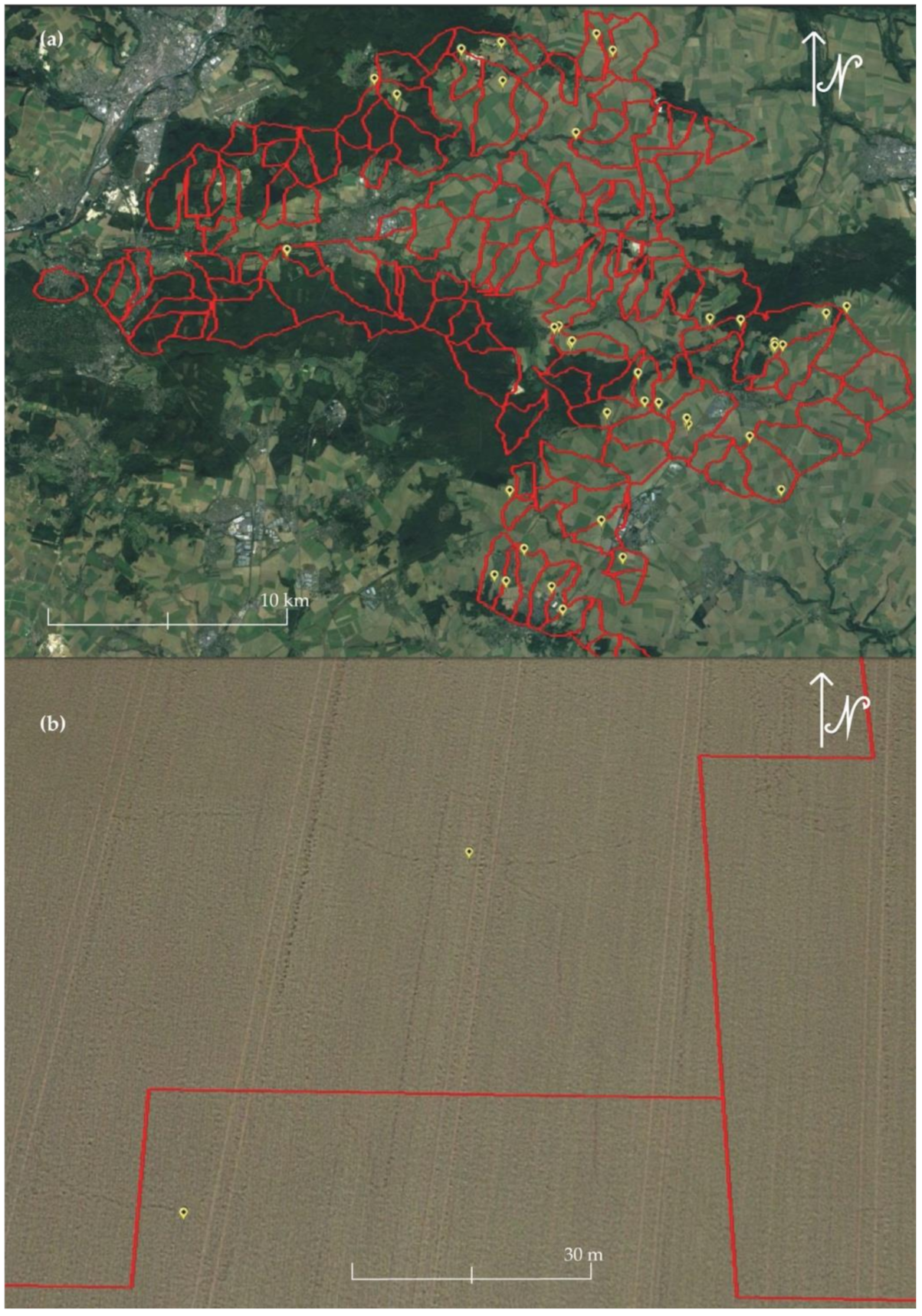
As seen above, 54% of the Nonette catchment is covered with non-irrigated arable land. These open fields are mainly found on the plateau or near the zone of steep slopes, which render them susceptible to erosion. Visible surface erosion activity has been mapped over the whole catchment (Figure 6). These marks left on the surface have been obtained through the digital reconnaissance of first-order catchments’ surface in Google Earth. To determine what marks were to be considered, information from Table 6 was used. During the survey, rills, gutter and ravines have been recognized; if present, claws remained invisible, probably due to their size, and no little ravines were observed. When a trace was visible within the limit of a first-order catchment, a small sign was added (in yellow in Figure 6) approximately where the trace was seen. If a catchment proved to have a mark, no further marks were sought, and the survey resumed. The aim of the survey was not to look for all the marks but to determine in which catchments these marks are found. For this reason, we do not provide an inventory here but a list of reactive catchments—catchments that have “responded” to an “excess” of erosion by the development of distinctive erosional forms on the surface.
Distinguishing between human-made tracks and visible surface erosion marks can prove difficult. The survey undertaken for this study has followed a simple methodology based on two criteria. The first is the use of multitemporal aerial pictures from Google Earth. In fact, if a mark was visible on pictures from different years, it was likely that the mark was human-made. The second criterion was the shape of the mark, together with its relation to the natural talweg determined in the pictures. If a mark was straight, it is likely that the mark was human-made; if the mark ran against the natural slope of the landscape, again, the mark could actually be human-made.
Out of the 122 Nonette first-order catchments, 40 catchments exhibit surficial silent witnesses of erosional activity (Figure 6). From Figure 6, one can see that reactive catchments are preferably encountered in the south-eastern and the northernmost parts of the catchment. In terms of geology, contact between the quaternary and the Bartonian seems to gather a great part of the reactive first-order catchments.
The specific degradation is the annual weight of alluvium carried by the water flow at the surface of the hydrographical basin, which integrates the whole load. This, however, is more particularly representative of volumes of suspended and dissolved matter, knowing that the bedload represents a tiny fraction of the total quantity of alluvium.
Generally, this value is comprised between one and over 50,000 tonnes per square kilometre per year (t·km−2·yr−1) [23]. For European rivers, this value ranges from 30 to 80 t·km−2·yr−1 [24]. Based on this assumption, the specific degradation of the Nonette catchment ranges between 11,790 and 31,440 t·yr−1.
However, this value can be further refined. Specifically, this range of value is coherent if the whole surface of the catchment contributes equally to the input of material into the stream. Based on Figure 6 and Table 6, this is not the case for the Nonette catchment, as about 50% of the headwaters’ catchments are covered by agriculture areas (in fact, after calculating the whole fourth-order catchment, this value nears 55%) One could argue that semi-agricultural land and forests could be considered too, but these areas’ roles are linked to the sinking and burial of material, rather than enhancing its mobility. Therefore, our assumption regarding the specific degradation of the Nonette catchment can be divided by 2, leading to a value ranging from 5895 to 15,720 t·yr−1.
We can assume that the whole load of material is uniformly distributed along the drainage line. In that case, between 21 and 56 t of material are accumulated for every kilometre of drainage line. This value is purely speculative, but can provide an estimate of the maximum quantity of material along a kilometre-long reach of the river.
Furthermore, the estimate made above is justified by the fact that few data, able to be extrapolated to the Nonette catchment, exist. In fact, after a bibliographical review, it appears that the Paris basin has mainly been studied (from the point of view of specific degradation) in its western part [25], and that the values given are 16 and 21 t·km−2·yr−1 for the Austreberthe and Andelle basins. In France, for the Royeau basin (Le Mans region), this value has been evaluated at 57 t·km−2·yr−1 [26], whereas the Caux country [27] presents values that vary between 140 and 240 t·km−2·yr−1. In Lower Normandy, the Traspy basin is given an average value of 60 t·km−2·yr−1 [28].
In view of the different specific degradation values encountered during this research, it appears that this value is dependent on geological substratum [29], anthropic activity [30] and climate [31], but also on catchment size (Table 1 in [25]); the differences from one catchment to another can be significant [32]. In order to refine the value of the specific degradation of the Nonette catchment, it is strongly recommended that an experimental study be carried out in situ, which in the long term could account for the erosive activity witnessed within the catchment and make it possible to quantify the annual material passing through the GC.

3. Numerical Modelling on a Local Scale

3.1. Material and Methods

3.1.1. Hydraulic System Description

The numerical model represents the GC of the Chantilly domain. The Nonette River is divided into two streams upstream of this domain by distribution work situated between the municipalities of Avilly-Saint-Léonard and Vineuil-Saint-Firmin, directly upstream from Avilly-Saint-Léonard’s former nail factory. This distribution work function was to manage the Nonette’s flow. Nowadays, the flow avoids the nail factory and reaches the Nonette River through an intermediary spillway. Further away, the Nonette flow gathers in the Hexagon. GC water flows toward the Manse Pavilion through a valved threshold equipped with a grid. The old locks have been condemned.
The hydraulic peculiarities found along the GC are identified in Figure 7. The model only represents the GC of the Chantilly domain. The Canal des Morfondus and the secondary canals of the English garden and the English–Chinese garden are not modelled.
The dam downstream of the Hexagon was erected in 2007, during dredging operations. Its aim is to reduce the sedimentary deposits in the GC [33]. The scaling takes into consideration a 15 cm water slide above the dam’s crest in normal functioning conditions. This mark is retained for the building of the numerical model.
The general dimensions of the different parts of the GC have been obtained from available plans found at Chantilly Castle library and archives, as well as in documents brought to the attention to the authors by the Nonette Basin Management Plan Interdepartmental Union (Table 7).

3.1.2. Model Building

HEC-RAS was developed by the U.S. Army Corps of Engineers (USACE). It is free public domain software, and its executable code and documentation can be downloaded from the USACE’s website (https://www.hec.usace.army.mil/software/hec-ras/ accessed on 15 December 2019). This study uses HEC-RAS version 5.0.7, which was made available in March 2019. It allows a 1D modelling of a steady flow regime, the 1 and 2D modelling of an unsteady flow regime and the 1D modelling of sediment transport in rivers in a quasi-unsteady flow regime [34]. The quasi-unsteady flow regime represents a continuous hydrograph shaped as a succession of discrete steady flow regimes (histogram). Solid transport is calculated for each steady flow regime’s segment.
Water streams’ geometry representation in HEC-RAS is based on transverse profiles. Cartesian coordinates (x, y, z) of profile points can be imported as a comma-separated values (CSV) file, where the horizontal position is measured by the distance to the true left bank (Station) and the vertical position is measured by the elevation of the corresponding point.
Geometrical data extracted from the documents gathered from partners establish an ensemble of mathematical and parametrical relationships. They are implemented through a VBA code in order to calculate the point coordinates from the profiles in Microsoft ExcelTM. The global geometry obtained is presented in Figure 1. The hydraulic system path is divided into three segments (or reaches) (Table 8).
The walls of the GC are considered as vertical walls (Figure 8). Their rugosity is modelled by the Manning coefficient, which is fixed at 0.022 (standard value for canals with deposits or vegetation, or raw rubble stones assembled with cement [35]).
The last sediment-dredging operations were performed in order to leave a water depth of 1.21 m in normal conditions [37]. This depth has been retained for the initial water depth of the model, and the hydraulic facilities of the numerical model are configured accordingly (especially the weir coefficient at the exit of the GC).

3.1.3. Limits Conditions

Flow rate time series being used have been gathered from Banque Hydro [14]. First, the division of flow rates is determined between the two supply points of the system, namely the Hexagon and the Tête du Rond. This division is performed by the distribution work of the former nail factory. Accurate geometrical characteristics of the distribution work were not known when the study was carried out. Therefore, approximate dimensions are extrapolated from field observations. In order to propose a flow rate distribution usable for the modelling, a functioning hypothesis has been established on the basis of the dimensions of the three spillways participating in the water distribution in the GC. It is a simplified assumption which, due to a lack of more detailed information, does not account for the influence of the Neuve River. Table 9 presents the parameters used to calculate the flow rate distribution and its values.
The height of the crest of the Nonette spillway is 0.20 m higher than that of the crest of the nail factory spillway. The activation flow rate of the Nonette spillway is therefore assumed to be equal to that for which the height of the water level at the crest of the nail factory spillway corresponds to this difference in height. This flow rate is evaluated using a rectangular weir equation [38] applied to the nail factory spillway:
Q = μ C v 2 g B c h e 3 2 ,
where Q = flow rate (m3/s); μ = flow rate coefficient (-); C v = speed of approach coefficient (-); g = gravitational acceleration (9.81 m/s2); B c = nail factory spillway crest width (m); h e = effective water height (m).
μ = 2 3 0.602 + 0.075 h 1 p ,
where h 1 = water depth above the weir crest in free (unsubmerged) conditions (m); p = height between spillway base and crest (m), considered as equal to 1 m.
C v = H 1 h 1 3 2 1 ,
where H 1 = water depth above the weir crest in submerged conditions (m).
h e = h 1 + K h ,
where K h , generally around 1 mm, is a correction made to take into account the effects of viscosity and surface tension. Applying Equation (1) to the spillway of the nail factory gives a weir flow rate value of Qweir = 1.051 m3/s. The flow rates going through the spillways of the Tête du Rond, the nail factory and the Nonette, respectively QR, Qc et QN (m3/s), are evaluated by means of a proportional relationship between the widths of the crests:
Q R = Q t B R B R + B c i f   Q t Q threshold , Q t B R B R + B c + B N i f   Q t > Q threshold ,
Q c = Q t B c B R + B c i f   Q t Q threshold , Q t B c B R + B c + B N i f   Q t > Q threshold ,
Q N = 0 i f   Q t Q threshold , Q t B N B R + B c + B N i f   Q t > Q threshold ,
where BR, Bc and BN are the widths of, respectively, the spillways of the “Tête du Rond”, the nail factory and the Nonette River (m); Qt is the total flow rate of the Nonette River at the entrance of the distribution work (m3/s), gathered from Banque Hydro [14].
The flow rate into the Tête du Rond is therefore equal to QR, and the flow rate into the Hexagon is equal to Qc + QN.
In order to represent complete hydrological cycles, each simulation represents one year of operation. HEC-RAS represents the flow rate in a quasi-unsteady regime, in the form of histograms of 100 values at most. Standard years are therefore represented as a series of 73 values of mean flow rate over 5-day periods, and leap years as 61 values of mean flow rate over 6-day periods.
The hydrological years can be qualified according to the size of the overall flow transferred by the Nonette River. Banque Hydro [14] provides results of the statistical analysis of the flow rates, including quantiles. Three types of hydrological years are distinguished:
  • Standard year, whose average flow rate is closest to the median of average annual flow rates;
  • Dry year, with the lowest average flow rate;
  • Wet year, with the highest average flow rate.
Figure 9a shows the values of average annual flow rates available in Banque Hydro [14]. Typical years identified from these data on the basis of the above criteria are:
  • Standard year: 1987;
  • Dry year: 2010;
  • Wet year: 2001.
HEC-RAS models the sediment input in the form of a rating curve representing the TSS (Total Suspended Solids) concentration as a function of river flow at each point of entry into the hydraulic system. To establish this curve, data from measurements of the SS concentration in the Nonette River at Courteuil provided by [39] are used. The flow rate corresponding to each date of SS concentration measurement has been obtained from Banque Hydro [14]. These values are represented by the graph in Figure 9b. The scatter plot thus obtained is approximated by a linear regression, which is applied in HEC-RAS to model the concentration–flow rating curve.
The available data on the latest dredging operations indicate that 90% of the sediment has a diameter less than 50 μm [40]. A linear particle size distribution is extrapolated from this information and translated into HEC-RAS for modelling. The translation of this distribution in the HEC-RAS interface is shown in Figure 10.

3.2. Results

3.2.1. Sensibility to Time Discretization

The entry hydrogram time step for an annual simulation is 5 days. In order to evaluate the sensitivity of the calculation of the volume of sediment accumulated in the GC to the value of this time step, the result of the simulation of a 5-day period with a constant flow rate equal to the mean flow is compared to the result of the detailed simulation of the same period with a 2 h step. The period considered is 21–25 October 2001. Figure 11 shows the flow rate histogram with a 2 h time step over this period, used for the detailed simulation. The mean flow rate over this period is 3.87 m3/s.
The simulation of the average flow rate leads to an accumulated volume of material of 24.6 m3, with the simulation of the detailed flow rate to a volume of 25.9 m3. The latter results in an increase of 5.4% compared to the simulation of the average flow rate.

3.2.2. Typical Years

Figure 12 shows the calculated longitudinal profile of the deposition height upstream of the GC as of 6 January 1987 (blue line). This result indicates the formation of an initial deposition zone corresponding to the accumulation of material at the entrance of the Neuve River in the Tête du Rond. This accumulation is favoured by the decrease in flow velocity due to the widening of the channel section in the Tête du Rond.
Figure 12 also shows the calculated longitudinal profile of the deposition height upstream of the GC at the end of 1987 (red line). This result indicates that a secondary deposition zone has formed upstream of the initial deposition zone, due to additional material gathered from events following the formation of the initial deposition and the loss of flow energy caused by the initial deposit.
These results indicate that most of the material brought by the Neuve River is deposited in the Tête du Rond. Only a small part of it is transported to the Hexagon.
Figure 13 shows the calculated longitudinal profile of the deposition height downstream of the GC as of 31 December 1987. The maximum height of deposit is 7.5 cm at the entrance of the Nonette River into the Hexagon (not shown in Figure 13). This result shows the influence of the hydraulic singularities of the GC on the deposit. Graphs (a), (b) and (c) in Figure 13 show details of the deposition height profile in the vicinity of these singularities. Sudden changes in the cross-section of the flow cause irregularities: a slight scouring, followed by an increase in deposition. A reduction in deposition is observed immediately upstream and downstream of the dam (Figure 13a). The narrowing of the flow cross-section at the bridge over the D924 road causes an acceleration of the flow, hence resulting in less sedimentation (Figure 13c).
These results indicate that a large part of the material is deposited between the entrance of the Nonette River into the Hexagon and the Channel.
The volume accumulated in the GC at the end of the 1987 simulation is 368 m3.
The calculated deposit longitudinal profile is similar to that in 1987. The volume accumulated in the GC at the end of the 2001 simulation is 1352 m3.
The volume accumulated in the GC at the end of the 2010 simulation is 145 m3. These results show the significant variability of material transport depending on the hydrological regime.

3.2.3. 10-Year Modelling

Figure 14 shows the annual volumes of sediment accumulated in the GC obtained by simulating 10 years of the system’s functioning. The period 2001–2010 is chosen because it is the most recent complete decade of flow rate data, with the hydrometric data from 2011 to 2020 being incomplete.
Figure 15a,b show the longitudinal profile of the sediment deposition height upstream and downstream of the GC, respectively. These results are consistent with those in Figure 12a and Figure 13, obtained for a single standard year, in that the deposition heights calculated at the end of the decade are approximately 10 times higher than those of a single year.
The total accumulated volume obtained from the simulation from 2001 to 2010 is 3901 m3. The value corresponds to a volume of dry sediment and does not take into account, in particular, materials contributed by vegetation, by direct runoff into the GC, by discharges from rainwater networks, or by wind transport.

4. Conclusions

The aim of this study was to constrain the quantity of sediment that enters the GC of the domain of Chantilly. The authors performed a geoscientific reconnaissance at catchment scale and ran a numerical simulation (HEC-RAS) of the sediment transport within the GC. The domain of Chantilly is a French historical heritage site of international fame. The castle was rebuilt during the nineteenth century while its garden has remained mostly unchanged. Nowadays, the GC, which is of the utmost touristic importance for the domain, is confronted with a deterioration of its water quality, which has been enhanced by the uncontrolled proliferation of algae, due to an excess of sediment present within the GC. This problem, which has had consequences on the income of the domain, needed to be addressed and is the subject of a scientific contribution for the first time.
At the scale of the Nonette catchment, marks of erosion are found throughout its surface, and it was shown that sediment is not a limiting agent of the erosional activity. It was estimated that between 5895 and 15,720 tonnes of sediment reach the Nonette River every year. It directly contributes to the amount of sediment that is deposited into the GC, but the authors have yet to determine in what proportions. Moreover, the estimates need to be better refined and induce more catchment studies (from the Nonette catchment and other regional catchments). For these reasons, the authors suggest that studies tackling local specific degradation should be undertaken, and encourage these future studies to focus on the Basin of Paris catchments, as few data are available for this region.
At the scale of the GC, the numerical simulation showed that the deposition of sediment is favoured between the Tête du Rond and the Channel of the GC. Over the 2.5 km GC, it was found that 3901 m3 of sediment was deposited between 2001 and 2010.
This volume of sediment does not take into account the material brought in by vegetation, by direct runoff, by discharges from rainwater networks, nor by wind transport. An estimate of the flows corresponding to these inputs would make it possible to better represent the behaviour of the system and strengthen our estimates. Additionally, the model estimates the flow rate’s distribution between the Tête du Rond and the Hexagon inlets based on simplifying assumptions. Better knowledge of the operation of the nail factory’s distribution work, in particular a law of structural behaviour, would allow a more accurate estimation of this distribution. This knowledge could be obtained from hydrometric, limnometric and bathymetric measurements within the distribution structure, possibly supported by 3D modelling using numerical fluid mechanics tools. Finally, bathymetric measurements in the GC would make it possible to compare the modelling results with actual deposition heights.
The objectives of the study have been achieved, focusing on the problem at a local scale and considering the bigger (environmental) picture at a catchment scale. The authors suggest that such a combination should be the base of similar studies, regardless of the study area. Additionally, an understanding of the environment at local scale is essential; for this study, the local organizations proved useful in answering the questions the authors came across. The authors can only encourage the involvement of local organizations in such studies. Ultimately, the outcomes of studies similar to the one presented herein, are a valuable source of information for these organizations and can play a role in future management plans, at both local and catchment scale.

Author Contributions

Conceptualization, G.G.C. and F.L.; methodology, E.M. and G.G.C.; software, F.L.; validation, F.L. and O.B.; formal analysis, G.G.C., E.M.; investigation, G.G.C. and E.M.; resources, E.M. and O.B.; data curation, F.L.; writing—original draft preparation, G.G.C.; writing—review and editing, G.G.C., F.L. and E.M.; visualization, G.G.C.; supervision, O.B.; project administration, E.M.; funding acquisition, E.M. All authors have read and agreed to the published version of the manuscript.

Funding

This research was funded by Interreg North West Europe SURICATES project. The APC was funded by the University of Lille (UL).

Institutional Review Board Statement

Not applicable.

Informed Consent Statement

Not applicable.

Data Availability Statement

No new data were created or analyzed in this study. Data sharing is not applicable to this article.

Acknowledgments

The authors would like to acknowledge the Interreg North West Europe SURICATES project and its members. We also thank the domain of Chantilly’s estate manager (Monsieur Basset) and team for their welcome and making access to the site possible, and the Bibliothèque et Archives du Musée de Condé de Chantilly for accessing documents in storage in relation to the management of the domain’s canals. Madame Morvan from the Syndicat Interdépartemental du Schéma d’Aménagement et de gestion des eaux de la Nonette (SISN) is warmly thanked for field visits and for providing the authors with relevant information in relation to the Nonette catchment. We would also like to thank Colin Childes from the Castle Triathlon Series, who initiated the contact between the University of Lille and SISN. Finally, we thank two anonymous reviewers for their insightful comments and guidance.

Conflicts of Interest

The authors declare no conflict of interest. The funders had no role in the design of the study; in the collection, analyses, or interpretation of data; in the writing of the manuscript, or in the decision to publish the results.

References

  1. Bonner, V.; Brunner, G.; Jensen, M. HEC River Analysis System (HEC-RAS). In Proceedings of the National Conference on Hydraulic Engineering, Buffalo, NY, USA, 1–5 August 1994; pp. 376–380. [Google Scholar]
  2. Werner, M. Impact of grid size in GIS based flood extent mapping using a 1D flow model. Phys. Chem. Earth Part B Hydrol. Ocean. Atmos. 2001, 26, 517–522. [Google Scholar] [CrossRef]
  3. Horrit, M.; Bates, P. Evaluation of 1D and 2D numerical models for predicting river flood inundation. J. Hydrol. 2002, 268, 87–99. [Google Scholar] [CrossRef]
  4. Thompson, C.; Rhodes, E.; Croke, J. The storage of bed material in mountain stream channels as assessed using Optically Stimulated Luminescence dating. Geomorphology 2007, 87, 307–321. [Google Scholar] [CrossRef]
  5. Sennaoui, F.; Benabdesselman, T.; Saihia, A. Use of modelling for the renovation of drainage channels–The case of the Bouteldja plain in northeastern Algeria. J. Water Land Dev. 2019, 43, 1–8. [Google Scholar] [CrossRef] [Green Version]
  6. Ara Rahman, S.; Chakrabarty, D. Sediment transport modelling in an alluvial river with artificial neural network. J. Hydrol. 2020, 588, 588. [Google Scholar] [CrossRef]
  7. Greenbaum, N.; Schwarz, U.; Carling, P.; Bergman, N.; Mushkin, A.; Zituni, R.; Halevi, R.; Benito, G.; Porat, N. Frequency of boulders transport during large floods in hyperarid areas using paleoflood analysis—An example from the Negev Desert, Israel. Earth-Sci. Rev. 2020, 202. [Google Scholar] [CrossRef]
  8. Banque Hydro. Available online: http://hydro.eaufrance.fr (accessed on 21 February 2020).
  9. Brunet, M.F.; Le Pichon, X. Subsidence of the Paris Basin. J. Geophys. Res. 1982, 87, 8547–8560. [Google Scholar] [CrossRef]
  10. Averbush, O.; Piromallo, C. Is there a remnant Variscan subducted slab in the mantle beneath the Paris basin? Implications for the Variscan lithospheric delamination process and the Paris basin formation. Tectonophysics 2012, 558, 70–83. [Google Scholar] [CrossRef]
  11. Robin, C. Mesure Stratigraphique de la Déformation: Application à L’évolution Jurassique du Bassin de Paris. Ph.D. Thesis, Université de Rennes, Rennes, France, 1995. [Google Scholar]
  12. Guillocheau, F.; Robin, C.; Allemand, P.; Bourquin, S.; Brault, N.; Dromart, G.; Friedenberg, R.; Garcia, J.P.; Gaulier, J.M.; Gaumet, F.; et al. Meso-Cenozoic geodynamic evolution of the Paris Basin; 3D stratigraphic constraints. Geodin. Acta 2010, 13, 189–245. [Google Scholar] [CrossRef]
  13. Robin, C.; Guillocheau, F.; Allemand, P.; Bourquin, S.; Dromart, G.; Gaulier, J.M.; Prijac, C. Echelles de temps et d’espace du contrôle tectonique d’un bassin flexural intracratonique-le Bassin de Paris. Bull. Soc. Geéol. Fr. 2000, 171, 181–196. [Google Scholar] [CrossRef]
  14. Brais, J. Le Cénozoïque du Bassin de PARIS: Un Enregistrement Sédimentaire Haute Résolution des Déformations Lithosphériques en Régime de Faible Subsidence. Ph.D. Thesis, Université de Rennes, Rennes, France, 2015. [Google Scholar]
  15. IGN. BD Alti V2. 2017. Available online: https://geoservices.ign.fr/documentation/diffusion/telechargement-donneeslibres.html#bd-alti-25-m (accessed on 15 December 2019).
  16. ESRI. ArcGIS Desktop: Release 10; Environmental Systems Research Institute: Redlands, CA, USA, 2010. [Google Scholar]
  17. Strahler, A.N. Hypsometric (area-altitude) analysis of erosional topography. GSA Bull. 1952, 63, 1117–1142. [Google Scholar] [CrossRef]
  18. Meteoblue. Available online: http://meteoblue.com/ (accessed on 4 May 2020).
  19. IGN. Corine Land Cover. 2018. Available online: https://land.copernicus.eu/paneuropean/corine-land-cover/clc2018 (accessed on 15 December 2019).
  20. Dufour, J.; Gravier, J.; Larue, J.-P. Fortes pluies et érosion des sols. L’orage de Mai 1988 dans la Sarthe. Bull. l’Assoc. Géographes Français 1990, 2, 159–170. [Google Scholar] [CrossRef]
  21. Auzet, A.V.; Boiffin, J.; Papy, F.; Ludwig, B.; Maucorps, J. Rill erosion as a function of characteristics of cultivated catchments in the North of France. Catena 1993, 20, 41–62. [Google Scholar] [CrossRef]
  22. Auzet, A.V.; Boiffin, J.; Ludwig, D. Concentrated flow erosion in cultivated catchments: Influence of soil surface state. Earth Surf. Proc. Landf. 1995, 20, 759–767. [Google Scholar] [CrossRef]
  23. Bravard, J.P.; Petit, F. Les Cours D’eau, Dynamique du Système Fluvial, 1st ed.; Colin: Paris, France, 1997. [Google Scholar]
  24. Serrat, P. Genèse et Dynamique D’un Système Fluvial Méditerranéen: Le Bassin de l’Agly (France). Ph.D. Thesis, Université de Perpignan, Perpignan, France, 2000. [Google Scholar]
  25. Laignel, B.; Dupuis, E.; Durand, A.; Dupont, J.-P.; Hauchard, E.; Massei, N. Erosion balance in the watersheds of the western Paris Basin by high-frequency monitoring of discharge and suspended sediment in surface water. CR Geosci. 2006, 338, 556–564. [Google Scholar] [CrossRef]
  26. Larue, J.-J. Runoff and interrill erosion on sandy soils under cultivation in the western Paris Basin: Mechanisms and an attempt at measurement. Earth Surf. Process. Landf. 2001, 26, 971–989. [Google Scholar] [CrossRef]
  27. Ouvry, J.-F. L’évolution de la grande culture et l’érosion des terres dans le Pays d Caux. Bull. l’Assoc. Géographes Français 1992, 2, 107–113. [Google Scholar] [CrossRef]
  28. Delahaye, D. Approches Spatialisées et Analyses Expérimentales des Phénomènes de Ruissellement et D’érosion des Sols. Ph.D. Thesis, Université de Caen, Caen, France, 1992. [Google Scholar]
  29. Agassi, M.; Lévy, G.J. Stone cover and rain intensity: Effects on infiltration, erosion and water splash. Soil Res. 1991, 29, 565–575. [Google Scholar] [CrossRef]
  30. Le Bissonnais, Y. Aggregate stability and assessment of soil crustability and erodibility: I. Theory and Methodology. J. Soil Sci. 1996, 47, 425–437. [Google Scholar] [CrossRef]
  31. Billard, A.; Cosandey, C.L.; Muxart, T. L’érosion sur les hautes terres du Lingas. In Mémoires et Documents de Géographie; CNRS: Paris, France, 1990. [Google Scholar]
  32. Le Bissonnais, Y. Analyse des Mécanismes de Désagrégation et de Mobilisation des Particules Sous L’action des Pluies. Ph.D. Thesis, Université d’Orléans, Orléans, France, 1988. [Google Scholar]
  33. AIRELE. Création d’un Barrage Sur le Grand Canal de Chantilly–Dossier de Déclaration au Titre de la Législation EAU; Technical Report; Château de Chantilly: Chantilly, France, 2007. [Google Scholar]
  34. Brunner, G.W. HEC-RAS, River Analysis System User’s Manual Version 5.0; Institute of Water Resources, Hydrological Engineering Center: Davis, CA, USA, 2016. [Google Scholar]
  35. Lencastre, A. Hydraulique Générale, 1st ed.; Eyrolles: Paris, France, 1999. [Google Scholar]
  36. Les Chênes Conseil. Parc du Château de Chantilly; Technical Report; Château de Chantilly: Chantilly, France, 2006. [Google Scholar]
  37. AIRELE. Etudes Préalables Aux Opérations de Curage sur le Grand Canal–Analyse du Projet, Programme Proposé, Étude D’incidences; Technical Report; Château de Chantilly: Chantilly, France, 2005. [Google Scholar]
  38. Ladreyt, S.; Laborie, V. Notice sur les Déversoirs: Synthèse des Lois D’écoulement au Droit des Seuils et Déversoirs, 1st ed.; Cerema (ex-Cetmef): France, 2005; Available online: https://side.developpement-durable.gouv.fr/Default/doc/SYRACUSE/223387/notice-sur-les-deversoirs-synthese-des-lois-d-ecoulement-au-droit-des-seuils-et-deversoirs (accessed on 20 July 2021).
  39. Naïades. Available online: http://naiades.eaufrance.fr/ (accessed on 21 February 2020).
  40. AIRELE. Présentation des Opérations de Curage du Grand Canal du Parc du Château de Chantilly; Technical Report; Château de Chantilly: Chantilly, France, 2008. [Google Scholar]
Figure 1. Nonette catchment with the three main rivers: Nonette, Aunette and Launette. C refers to Chantilly domain and S to the city of Senlis.
Water 13 01989 g001
Figure 2. Mean monthly flow rate calculated over a 41-year period at Courteuil hydrological station, after [8].
Water 13 01989 g002
Figure 3. Geological map of the Nonette catchment.
Water 13 01989 g003
Figure 4. (a) Digital elevation model of Nonette catchment; (b) slope raster of Nonette catchment.
Water 13 01989 g004
Figure 5. Soil use based on CLC [19] visualized together with the 122 1st-order catchments within the Nonette catchment.
Water 13 01989 g005
Figure 6. (a) Surficial silent witnesses on the scale of Nonette catchment; (b) zoom on the type of surficial silent witnesses distinguished from aerial pictures (Google Earth) survey.
Water 13 01989 g006
Figure 7. Situation of Chantilly domain (Google Earth); bird’s-eye view from the GC; geometry represented in HEC-RAS and hydraulic peculiarities along the GC.
Water 13 01989 g007
Figure 8. Structural scheme of GC walls, reproduced after [36].
Water 13 01989 g008
Figure 9. (a) Yearly mean flow rates from 1969 to 2016 [13]; red crosses show the typical years used for modelling. (b) Suspended solid concentrations as a function of the flow rate (values from [14,38,39]); linear regression used for modelling.
Water 13 01989 g009
Figure 10. HEC-RAS granulometric distribution; grain size in mm on the x-axis and sieve in percentage (%) on the y-axis.
Water 13 01989 g010
Figure 11. Flow rate histogram between 21–25 October 2001, with a 2 h time step.
Water 13 01989 g011
Figure 12. Calculated longitudinal profile of the deposition height upstream of GC on 6 January 1987.
Water 13 01989 g012
Figure 13. Calculated longitudinal profile of the deposition height downstream of the GC on 31 December 1987. (a) Details of the calculated longitudinal profile between the Hexagon exit and the dam. (b) Details of the calculated longitudinal profile in the vicinity of the Channel. (c) Details of the calculated longitudinal profile at the bridge.
Water 13 01989 g013
Figure 14. Annual sediments volumes accumulated in GC and obtained from the 10-year modelling.
Water 13 01989 g014
Figure 15. Calculated longitudinal profile of the deposition height at the end of 2001–2010 decade. (a) Upstream of the GC; (b) downstream of the GC.
Water 13 01989 g015
Table 1. Morphometrical parameters chosen for the Nonette catchment’s characterization with unit, the equation, if it is applied to the catchment or the stream and the results; C stands for catchment; S for stream. To be noted that « L » defined for the form factor corresponds to the length of the best-fitted ellipsoid calculated through the zonal geometry as table tool in the geographic information system (GIS).
ParameterUnitEquationApplied toResults (C/S)
Areakm2(-)C393.8
Perimeterkm(-)C180
Elevation maxm asl(-)C/S222/138
Elevation minm asl(-)C/S25/25
Elevation meanm asl(-)C/S93.30/77.71
Slope max/mindegrees(-)C/S29.69/0/16.16/0
Slope meandegrees(-)C/S1.66/1.07
Lengthkm(-)S278.9
Melton ratio(-) d H A C0.01
Form factor(-) A L 2 C0.50
Elongation(-) 2 A L π C1.60
Table 2. Morphometrical results associated with catchments and encompassing area (km2), perimeter (km), elevations (m asl) and slopes (°). Results are to be understood as follows: minimum/maximum/mean.
Parameter1st-Order Catchments2nd-Order Catchments3rd-Order Catchments
Area1.01/8.3/2.33.24/21.8/9.417.2/102/70.6
Perimeter4.7/23.8/9.29.7/31.8/18.127/75.9/57.8
Elevation max58/222/127.166/222/147.9110/222/173
Elevation mean44/154.1/96.756/125.2/9861/110/94
Elevation min28/116/76.735/100/70.640/64/53
Slope max2/25.3/10.61.3/11.6/49/25/18
Slope mean0/5.17/1.700.4/1.38/0.931/2/2
Slope min0/0/00/0/00/0/0
Table 3. Morphometrical results associated with streams and encompassing length (km), elevations (m asl) and slopes (°).
Parameter1st-Order Streams2nd-Order Streams3rd-Order Streams
Length0.175/0.95/0.3851.5/15.6/5.99.6/71.7/49.8
Elevation max30/138/8644/138/9564/138/110
Elevation mean29/120.5/81.238/112.6/82.353/93/80
Elevation min28/116/76.835/100/70.640/64/53
Slope max0/10.1/2.531.3/11.6/44/16/9
Slope mean0/6.3/10.4/1.38/0.931/1/1
Slope min0/6/0.170/0/00/0/0
Table 4. Morphometrical results associated with catchments that encompass Melton ratio, form factor and basin elongation.
Parameter1st-Order Streams2nd-Order Streams3rd-Order Streams
Melton ratio0.01/0.1/0.040.01/0.05/0.030.01/0.017/0.015
Form factor0.2/0.75/0.40.3/0.66/0.470.347/0436/0.394
Basin elongation0.98/1.96/1.421.2/1.84/1.541.330/1.491/1.416
Table 5. Details of the CLC classes found within Nonette’s 122 1st-order catchments.
CLC LabelCLC ClassCoverage Percentage
112Discontinuous urban fabric5.23
121Industrial or commercial units1.00
122Road and rail networks and associated land0.36
124Airports0.09
131Mineral extraction sites0.18
132Dump sites0.08
133Construction sites0.13
142Sport and leisure facilities3.01
211Non-irrigated arable land54.01
222Fruit trees and berry plantations0.11
231Pastures1.56
242Complex cultivation patterns0.65
243Land principally occupied by agriculture0.26
311Broad-leaved forest24.08
312Coniferous forest4.56
313Mixed forest5.92
324Transitional0.55
112Discontinuous urban fabric5.23
Table 6. Distinctions between soil erosion forms as a function of their size [20,21,22].
FormsShapeLengthWidthSlopeSituation
ClawSinuous<1 m<10 cm>1%Hillside
Rill/inter-rillStraight~100 m10–20 cm>3%Hillside
GutterSinuous~10 m5–80 cm>3%Hillside/Talweg
RavineSlightly sinuous~100 m50 cm–100 cm<6%Talweg
GullySlightly sinuous~100 m>50 cm<6%Talweg
Table 7. General dimensions of the hydraulic system used in HEC-RAS.
Main Hydraulic System PartsDimensions
Length of the GC2677 m
Mean slope of the GC0.0027%
Wall height2 m
Tête du rond radius59 m
Maximum breadth of the Hexagon218 m
Maximum breadth of the Channel318 m
Breadth of GC Segments 1 and 263 m
Breadth of GC Segment 356 m
Table 8. Description of the three hydraulic system segments modelled.
Name of ReachDescription
GC—upstreamPortion of the stream between the Neuve River arrival into the Tête du Rond and just upstream of the entry of the Nonette River into the Hexagon
NonetteSegment of the Nonette River inlet into the Hexagon
GC—downstreamPortion of the stream between just downstream of the entry of the Nonette River into the Hexagon and the GC outlet
Table 9. Parameter values used to assess the flow rate distribution between the Hexagon and the Tête du Rond.
ParameterValueIn Equation (1)
Width of the nail factory spillway1.7 mB
Width of Nonette River spillway7.3 m
Difference in elevation between nail factory spillway crest and Nonette River spillway+0.2 mh1
Width of Tête du Rond spillway4.7 m
Height between GC bottom and nail factory spillway crest1 mp
Publisher’s Note: MDPI stays neutral with regard to jurisdictional claims in published maps and institutional affiliations.

